Corrigendum: Mesozooplankton and Micronekton Active Carbon Transport in Contrasting Eddies
 Lian E. Kwong
 Natasha Henschke
 Evgeny A. Pakhomov
 Jason D. Everett
 Iain M. Suthers
- 1Department of Earth, Ocean and Atmospheric Sciences, University of British Columbia, Vancouver, BC, Canada
- 2Institute for the Oceans and Fisheries, University of British Columbia, Vancouver, BC, Canada
- 3Hakai Institute, Heriot Bay, BC, Canada
- 4Centre for Applications in Natural Resource Mathematics, The University of Queensland, St. Lucia, QLD, Australia
- 5Evolution and Ecology Research Centre, University of New South Wales Sydney, Sydney, NSW, Australia
- 6Sydney Institute of Marine Science, Mosman, NSW, Australia
Mesozooplankton (June 2015 and September 2017) and micronekton (September 2017) were sampled along the eastern coast of Australia. Depth stratified mesozooplankton and micronekton were collected using a Multiple Opening/Closing Net and Environmental Sensing System (MOCNESS) and an International Young Gadoid Pelagic Trawl (IYGPT) equipped with an opening/closing codend. Sampling was undertaken at the center and edge of a frontal cold-core eddy (F-CCE Center and Edge) in 2015, and at the center of a cold-core eddy (B-CCE) and two warm-core eddies (R-WCE and WCE) in 2017. We assess the diel vertical structure, biomass, and downward active carbon transport by mesozooplankton and micronekton in eddies. Total water column mesozooplankton and micronekton biomass did not vary substantially across water masses, while the extent and depth of diel vertical migration did. Using in situ measurements of temperature and measurements of mesozooplankton and micronekton abundance and biomass, we estimated the contribution of respiration, dissolved organic carbon (DOC) excretion, gut flux, and mortality to total downward active carbon transport in each water mass. Overall, active carbon transport by mesozooplankton and micronekton below the mixed layer varied substantially across water masses. We corrected estimates of micronekton migratory biomass and active carbon transport assuming 50% net efficiency. In the R-WCE mesozooplankton remained within the mixed layer during the day and night; only 50% of the total micronekton population migrated below the mixed layer contributing to carbon transport, equating to 2.89 mg C m–2 d–1. Mesozooplankton actively transported 16.1 and 8.0 mg C m–2 d–1 at the F-CCE Center and Edge, respectively. Mesozooplankton and micronekton active carbon transport in the B-CCE were 5.4 and 0.74 mg C m–2 d–1, and in the WCE 88 and 13.4 mg C m–2 d–1. Differences in carbon export were dependent on food availability, temperature, time spent migrating, and mixed layer depth. These findings suggest that under certain conditions mesoscale eddies can act as important carbon sinks.
Introduction
The planktivorous mesopelagic fishes arguably have the Earth’s largest fish biomass, which is likely underestimated by an order of magnitude due in part to the unknown energy transfer through the zooplankton component of pelagic food webs (Irigoien et al., 2014). Energy fluxes between the epipelagic (<200 m) and the mesopelagic (200–1000 m) layers vary globally and play a key role in determining marine productivity and fisheries (Young et al., 2011, 2015; Kiko et al., 2017; Reygondeau et al., 2017). The permanent mesopelagic inhabitants (non-vertical migrators) rely on both the passive sinking of epipelagic particles and migratory organisms as a food source, although the proportional importance is still debated (Hannides et al., 2013; Choy et al., 2015). Due to surface waters warming, epipelagic productivity and vertical energy flux dynamics are expected to change as animals retreat to cooler waters resulting in vertical and/or latitudinal shifts (Poloczanska et al., 2016). Therefore, resolving the factors that influence vertical energy flux is central to understanding the implications of environmental change on commercially valuable fisheries and vertical carbon flux.
Mesozooplankton (0.2–20 mm) and micronekton (20–200 mm) undergo extensive diel vertical migrations (DVMs), feeding in the highly productive surface waters at night and migrating back down to depth during the day where they reside to avoid predation (Iwasa, 1982; Hays et al., 1997) and improve metabolism (McLaren, 1974; Enright, 1977; Iwasa, 1982; Hernández-León et al., 2010). Depending on the assemblages and their body size, they can migrate to depths of 500–1000 m (Baird et al., 1975; Irigoien et al., 2014). Once at depth, these organisms metabolize surface-derived nutrients releasing carbon by way of respiration, dissolved organic carbon (DOC) excretion, gut flux, and mortality (Steinberg et al., 2000; Ducklow et al., 2001; Davison et al., 2013; Steinberg and Landry, 2017). As these processes are largely size, temperature, and pressure dependent they can therefore be calculated for whole communities by applying a size-based approach (Zhang and Dam, 1997; Steinberg et al., 2000; Ikeda, 2013a, 2014, 2016). Larger organisms likely transport more carbon due to their deeper migrations (Sameoto et al., 1987; Moteki et al., 2009), body size/mass (Hansen and Visser, 2016), large fecal pellets (Turner, 2002), and long gut passage times (GPTs) (Baird et al., 1975; Dagg and Wyman, 1983; Reinfelder and Fisher, 1994; Pakhomov et al., 1996).
The importance of vertically migrating zooplankton and micronekton to biogeochemical cycling is becoming increasingly apparent, although it remains largely unquantified (Tsubota et al., 1999; Hansen and Visser, 2016; Gorgues et al., 2019). Most studies focus on specific aspects of active carbon transport such as the respiration, DOC excretion, gut flux, and/or mortality of individual species (Kobari et al., 2008), groups (i.e., orders or classes of zooplankton and micronekton; Hidaka et al., 2001; Davison et al., 2013) or specific size ranges (e.g., 0.1–1 mm total length; Hernández-León et al., 2001; Davison et al., 2013; Ariza et al., 2015). It is rare that all fluxes (i.e., respiration, DOC excretion, gut flux, and mortality) are considered when estimating active carbon transport via mesozooplankton and micronekton (Steinberg and Landry, 2017). By neglecting certain species/taxa, sizes, or fluxes, we are underestimating carbon export to the deep ocean, leading to inconsistencies between models (Falkowski et al., 2003; Usbeck et al., 2003; Martz et al., 2008; Davison et al., 2013). There remains a high uncertainty in active carbon transport estimates stemming largely from methodological approaches and spatial variability (Steinberg and Landry, 2017).
Distinct biological communities develop in mesoscale eddies, which are particularly effective at retaining and transporting organisms that undergo DVM (Mackas and Galbraith, 2002). Within eddies, differences in phytoplankton composition and zooplankton biomass, respiration, and fecal pellet production have been observed between the center and periphery of eddies (Mackas and Coyle, 2005; Yebra et al., 2005; Goldthwait and Steinberg, 2008; Landry et al., 2008). To our knowledge only four studies have looked at the effects of mesoscale eddies on active carbon transport (Yebra et al., 2005, 2018; Landry et al., 2008; Shatova et al., 2012). These studies looked at specific fluxes (i.e., gut flux and respiratory flux) by mesozooplankton. No studies have looked at the contribution of micronekton to carbon transport, though some suggest that micronekton aggregate in and around eddy centers (Sabarros et al., 2009; Drazen et al., 2011).
In the southwestern Pacific Ocean, there are no studies that look at active carbon transport of both mesozooplankton and micronekton within or across eddies, but one study assessed the contribution of pelagic tunicates (Henschke et al., 2019). Some mesozooplankton and micronekton studies have focused on the subtropical convergence off eastern Tasmania (Young and Blaber, 1986; Young et al., 1987, 1988), while the mesozooplankton and micronekton communities in the temperate Tasman Sea are comparatively understudied. Changes in zooplankton communities have been observed off southeastern Australia as a result of a southerly extension of the East Australian Current (EAC) and its eddy field, with continued changes likely to have impacts on pelagic fish and fisheries in the area (Hobday et al., 2011; Kelly et al., 2016).
In the southwest Pacific, the EAC transports warm, tropical water southwards along the coast until it diverges eastward at ∼32°S (Suthers et al., 2011; Cetina-Heredia et al., 2014). Associated with the EAC is a dynamic mesoscale eddy field, where frequent cyclonic (cold-core) and anti-cyclonic (warm-core) eddies are formed (Everett et al., 2012). Generally, cold-core eddies in this region have been found to create more productive pelagic habitats compared to warm-core eddies (Greenwood et al., 2007; Everett et al., 2012). The pelagic environments of cold- and warm-core eddies are often different to each other, and to the surrounding water due to a range of eddy-driven processes such as entrainment (Greenwood et al., 2007; Everett et al., 2015), eddy induced Ekman pumping (McGillicuddy and Robinson, 1997; Martin and Richards, 2001), or eddy trapping (Chenillat et al., 2018).
In this study, our overall goal was to compare the biomass, diel-vertical migration, and vertical fluxes of mesozooplankton and micronekton communities across a range of eddy environments along the eastern coast of Australia during the winter of 2015 and the spring of 2017. Specifically, our aims were to (a) assess the diel vertical structure of mesozooplankton and micronekton biomass between eddies, and to (b) quantify downward active carbon transport mediated by mesozooplankton and micronekton.
Materials and Methods
Study Area
Sampling was undertaken from the RV Investigator in the western Tasman Sea during winter (2–18 June 2015) and spring (6–15 September 2017) voyages. The sampling area extended from Brisbane (27.5°S) south to Batemans Bay (35.7°S; Figure 1). The hydrographic features in the region were identified using a combination of satellite-derived chlorophyll a [Moderate Resolution Imaging Spectroradiometer; MODIS-Aqua via Integrated Marine Observing System (IMOS)], sea-surface temperature (MODIS-Aqua via IMOS1), and altimetry (IMOS and bathymetry data; General Bathymetric Chart of the Oceans; GEBCO).
FIGURE 1

Figure 1. Southeast coast of Australia (A) highlighting the 2015 (red) and 2017 (white) sampling locations with bathymetry overlaid. For 2015 (top) the F-CCE location (∘) is shown with (B) Sea Surface Temperature (SST) and ADCP data (Roughan et al., 2017), and (C) chlorophyll a (Chl. a) data from the 8–9 June 2015. For 2017 (bottom) the locations of the B-CCE (□), R-WCE (⋄), and WCE (Δ) are shown with (D) SST and altimetry data from IMOS, and (B) Chl. a data from the 3–5 September 2017. The black line represents the 200 m shelf (B–E).
Five water types were sampled during this study. In June 2015, the center and the edge of an ∼35 km frontal cold-core eddy (“F-CCE”) was sampled off Forster (∼33°S; Figures 1B,C). This productive eddy formed adjacent to the continental shelf a week prior to sampling, entraining shelf water, before moving off the shelf into the warmer EAC (Roughan et al., 2017). In September 2017, three eddies were sampled (Figures 1D,E): an ∼150 km cold-core eddy off Brisbane (∼27.5°S; “B-CCE”), a large (∼200 km) warm-core eddy (WCE) that formed from the retroflection of the EAC (∼33°S; R-WCE), and an ∼150 km WCE sampled south of the Tasman Front (∼35°S) that was also formed from EAC water (Henschke et al., 2019).
Eddies were identified using a combination of satellite SST and altimetry, and an onboard Acoustic Doppler Current Profiler (ADCP). The 2015 F-CCE was too small to be visible using altimetry, but was clearly visible in SST, and verified using the ADCP (Figure 1B). The 2017 eddies were all large enough to be observed using satellite altimetry (Figure 1D).
Oceanographic Sampling
At each eddy a Seabird SBE911-plus Conductivity–Temperature–Depth (CTD) probe equipped with a calibrated Chelsea Aqua-Tracker Mk3 fluorometer and fitted with 12 L bottles on a rosette sampler was used to profile temperature, salinity, and fluorescence. Mixed later depth (MLD) for each eddy was calculated following Levitus (1982) as the depth at which σT > surface σT + 0.125, where σT is the density. Water samples taken from the rosette at various depths were used to measure nutrients and calibrate oxygen and chlorophyll a from the CTD. Dissolved inorganic nutrient measurements were made using automated continuous flow with colorimetric detection following CSIRO standard operating procedures (Rees et al., 2018). Fluorescence was converted to chlorophyll a concentrations through regression analyses as described in Roughan et al. (2017) for 2015 samples (r2 = 0.81, n = 66) and Henschke et al. (2019) for 2017 samples (r2 = 0.84, n = 20) to provide full water column chlorophyll a estimates. Dissolved oxygen concentrations were determined using the Winkler-titration method (Strickland and Parsons, 1972).
Mesozooplankton (June 2015 and September 2017) and micronekton (September 2017) sampling was concentrated in the eddy centers. Additional mesozooplankton sampling was undertaken outside the eddy in 2015 (Supplementary Table S1).
Mesozooplankton
Depth-stratified sampling for mesozooplankton was undertaken during the day and night using a Multiple Open-Closing Net and Environmental Sensing System (MOCNESS). The MOCNESS had a mouth-opening of 1 m2 and consisted of five nets that can be triggered remotely, all fitted with 500 μm mesh. The MOCNESS was lowered to 500 m and five oblique tows were performed while the vessel was traveling at 1.5 m s–1: 500–400, 400–300, 300–200, 200–100, and 100 m to the surface. Immediately after collection, approximate mesozooplankton size classes were determined by gently rinsing the contents of each cod-end through a sieve column to four size classes: 500–1000, 1000–2000, 2000–4000, and >4000 μm. All organisms that were >4000 μm were individually measured, counted, and grouped into two additional logarithmic size classes: 4000–8000 and 8000–16,000 μm. The groups were placed onto pre-weighed petri dishes, oven dried at 50°C, and weighed to the nearest 0.01 g. Dry weight was converted to carbon weight (mg C m–3) assuming carbon weight = 0.4 ∗ dry weight (Parsons et al., 1984; Steinberg et al., 2000). Total biomass (mg C m–3) for each tow was total carbon weight captured in each tow divided by volume filtered. Abundance of each size fraction was calculated as follows. A representative biovolume for an animal equal to the mid-size of the size-fraction was calculated by assuming ellipsoid shape and near-neutral density following Suthers et al. (2004). Wet weights were then converted to dry weight assuming dry weight = 0.1 ∗ wet weight (Weibe et al., 1975). Finally, we calculated total mesozooplankton abundance in each size-fraction (i.e., counts per tow) by dividing total dry weight of the size fraction by the mean animal dry mass.
Volume of water filtered was calculated using the G.O. mechanical flow meter (General Oceanics Inc., Miami, United States) mounted on the MOCNESS.
Micronekton
In 2017, additional sampling was undertaken to quantify micronekton (20–200 mm) biomass in each eddy using a 157.5-m2 International Young Gadoid Pelagic Trawl (IYGPT). Mesh size of the trawl reduced from 200 mm stretched mesh width at the mouth to 10 mm in the codend. The trawl was equipped with a MID water Open and Closing net system (MIDOC; Marouchos et al., 2017), with a 1-m2 mouth area and six cod-ends graduating from 10 mm mesh to 500 μm mesh. The MIDOC was lowered to two target depths (500 and 1000 m) during both the day and night while the vessel maintained a speed of 1 m s–1. We employed two different depth stratified sampling strategies: (1) 1000–900, 900–800, 800–700, 700–600, 600–500, and 500–0 m, and (2) 0–500, 500–400, 400–300, 300–200, 200–100, and 100–0 m. Each depth stratum was sampled for ∼20–40 min (Supplementary Table S1). The volume of water filtered was calculated based on the spread and height of the MIDOC doors and the distance traveled through the water column.
Immediately after collection, micronekton were separated into major taxonomic groups, identified to the lowest possible taxonomic level, counted, individually weighed, and photographed for body length (mm). The major taxonomic groups included myctophids, decapods, and cephalopods (for a complete species list, see Supplementary Table S2). We did not include gelatinous organisms (i.e., siphophores, jellyfish, and salps) in our analysis, as they were often damaged in net tows. Carbon weights were calculated using individual lengths and length to weight relationships (LWRs) from the literature or FishBase Bayesian LWR (Froese et al., 2014), by directly weighing the individuals, or by using the average LWR of the genus or family (Supplementary Table S3). Where no direct carbon weight to wet weight relationship was available, we assumed carbon weight = 20% of wet weight (Crabtree, 1995; Andersen et al., 2016). Abundance for each size class (mesozooplankton) and taxon (micronekton) was determined by dividing the number of individuals captured in each tow by the volume of water filtered.
For our analysis, we include organisms from the MOCNESS ranging from 0.5 to 16 mm in size and from the MIDOC 20 to 200 mm total length. All values are reported as mean ± standard error (S.E.).
Data Analysis
To test the day and night differences in mesozooplankton and micronekton biomass at each eddy we applied ANOVA, but first tested the assumptions using Bartlett’s test (homogeneity of variance) and Shapiro–Wilk test (normality) using R Statistical Software (R Core Team). All statistical values are reported in Supplementary Tables S4, S5.
Active Carbon Transport
The migratory community refers to the portion of mesozooplankton and micronekton that actively migrate into the mixed layer during the night to feed and reside below the mixed layer during the day. This portion of the community was calculated based on day and night differences in biomass within the mixed layer. Thus, only the biomass migrating below the MLD were included in our calculation of downward active carbon flux at each location. Organisms that do not migrate below the MLD instead contribute to carbon “recycling” within the MLD, whereby, they consume organic matter and respire, excrete, die, and produce fecal pellets that remain within the MLD.
To determine depth of vertical migration, we calculated the weighted mean depth (WMD, m) for each taxonomic group as follows:
where bji is the biomass (mg CW m–3) and dji is the midpoint of the depth stratum (m) for taxon j in each sampling location (i).
For mesozooplankton we infer total abundance (N) in each size bin using geomean carbon weight (GM; mg ind.–1), which represents mean carbon weight of an individual (ind.) in size bin x, and total carbon weight (CW; mg) within size bin x as follows:
To calculate the contribution of mesozooplankton and micronekton to active carbon transport, we must first calculate individual respiration, DOC excretion, gut flux (defecation), and mortality. To do so, we calculate individual rate processes using size-dependent rate equations. Individual rates are then scaled up using migratory densities, and the depth of export is assumed using WMD. Finally, we also calculate the carbon flux to migratory biomass ratio for each group to assess the downward contribution per day.
Respiration
Respiratory oxygen uptake (RO; μL O2 ind.–1 h–1) was calculated using size, temperature, and taxon-specific rate equations (Supplementary Table S6). Respiratory oxygen uptake was converted into respiratory carbon equivalent (RC; μg C ind.–1 d–1) as follows:
where RQ is the respiratory quotient (Supplementary Table S6), 12 is the molar weight of carbon (g mol–1), 22.4 is the molar volume (mol L–1) of an ideal gas at standard pressure and temperature, and TD is the time spent at depth. Community respiration was then calculated by adding together individual respiration rates for each depth stratum.
Excretion
Dissolved organic carbon excretion was assumed to be 31% of CO2 respiration based on Steinberg et al. (2000). The study reported that DOC excretion was on average 31% of CO2 respiration (μg C respired) or 24% of the total metabolized carbon (i.e., excreted + respired), and found similar variation, depending on environmental temperature and organism weight, across crustacean species. We apply the same relationship for DOC excretion to myctophids, as estimates for fishes are lacking in the literature (Hudson et al., 2014).
Mortality
We apply two different approaches to calculate zooplankton and micronekton mortality to ease comparison with other studies, and to demonstrate the vast variability in estimates.
For our model, downward carbon flux arising from zooplankton and micronekton mortality was calculated based on the Zhang and Dam (1997) adaptation of Peterson and Wroblewski (1984). This approach assumes that predation scales in an isometric fashion.
where Mh is the hourly weight-specific mortality rate based on individual dry weight (DW; g). Mh can be multiplied by the number of hours spent at depth to obtain individual contribution to downward flux attributed to natural mortality.
For comparison, we also calculate mortality from growth as in Hernández-León et al. (2019). Assuming our systems are in steady-state, growth should be approximately equivalent to mortality. We calculate zooplankton growth according to Ikeda and Motoda (1978), where Growth = 0.75 ∗ Respiration. For micronekton, we use the growth/metabolism ratio (0.66) from Brett and Groves (1979).
Gut Flux
We assume that organisms migrating into the surface waters during the night are feeding to complete satiation, and use the average index of stomach fullness (ISF; dry weight of stomach contents/dry weight of organism) and organism size (DW; mg) to calculate food ball dry weight (FB; mg):
Taxon-specific estimates of mean ISF were compiled from the literature and are provided in Supplementary Table S7. Food ball dry weight is converted to carbon units assuming carbon weight = 0.4 ∗ dry weight (Parsons et al., 1984; Steinberg et al., 2000). We apply an assimilation efficiency of 88% to calculate the average carbon weight of the daily egested material (E; mg C d–1) (Hopkins and Baird, 1977). Assuming egestion is constant throughout the day, we divide daily egestion (E) by 24 h to obtain hourly egestion. To contribute to downward gut flux, GPT (Supplementary Table S7) must exceed the amount of time spent on downward migration (DM; h) (Table 1); where this is not the case (i.e., GPT ≤ DM) gut flux was automatically set to zero. Time spent on downward migration, at depth, and at the surface were estimated based on the acoustic backscatter from the onboard EK60 (Suthers, 2017). Therefore, total downward gut flux is:
TABLE 1
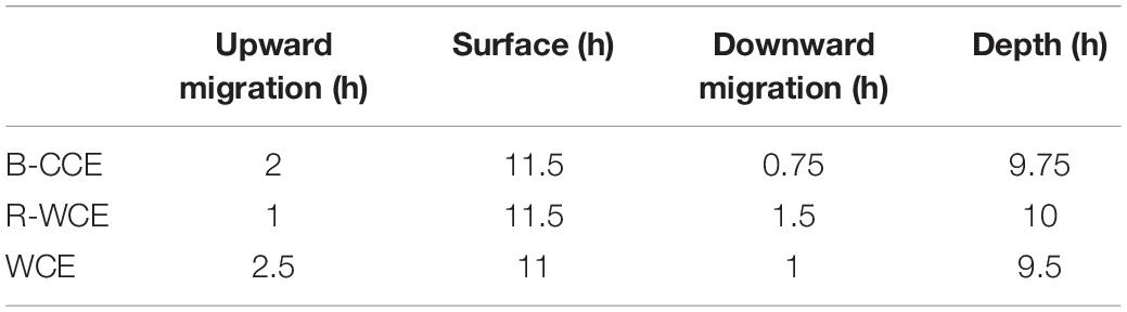
Table 1. Hours micronekton spent migrating upward, staying at the surface (night), migrating downward and staying at depth (day), and during diel vertical migrations derived from EK60.
Gut passage times (h) for the various taxa captured were compiled from the literature (Supplementary Table S7). Gut flux of polychaetes and mollusks was calculated assuming that they had the same ISF and GPT as copepods, as no specific estimates were available from the literature. Previous studies argue that pelagic mollusks exhibit similar feeding strategies as copepods, with short GPTs (Dagg and Wyman, 1983; Reinfelder and Fisher, 1994). For the MOCNESS data, copepods and mollusks made up the majority of the biomass. Therefore, we assume short GPTs (1.04 h; Dagg and Wyman, 1983; Reinfelder and Fisher, 1994). As no echogram is available for the 2015 voyage, we assume the downward migration at the F-CCE (center and edge) will be similar to that of the B-CCE (i.e., 0.75 h).
Results
Oceanographic Setting
The F-CCE Center (58 m) and F-CCE Edge (102 m) had shallow mixed layers (Figure 2A) and temperature and salinity profiles were characteristic of shelf water and EAC water, respectively (Roughan et al., 2017). The F-CCE Center was less saline and had significantly higher chlorophyll a concentrations (0.96 ± 0.12; F4,29 = 82.66, p < 0.001) in the surface layer (0–50 m) compared to other water masses. Nutrient levels were low in surface waters, but increased rapidly from 50 m. In comparison, the F-CCE Edge was more saline, warmer, and had lower chlorophyll a and nutrient concentrations than the F-CCE Center. Dissolved oxygen declined sharply below the mixed layer to minimums near 100 (Center) and 150 m (Edge) (Figure 2E).
FIGURE 2
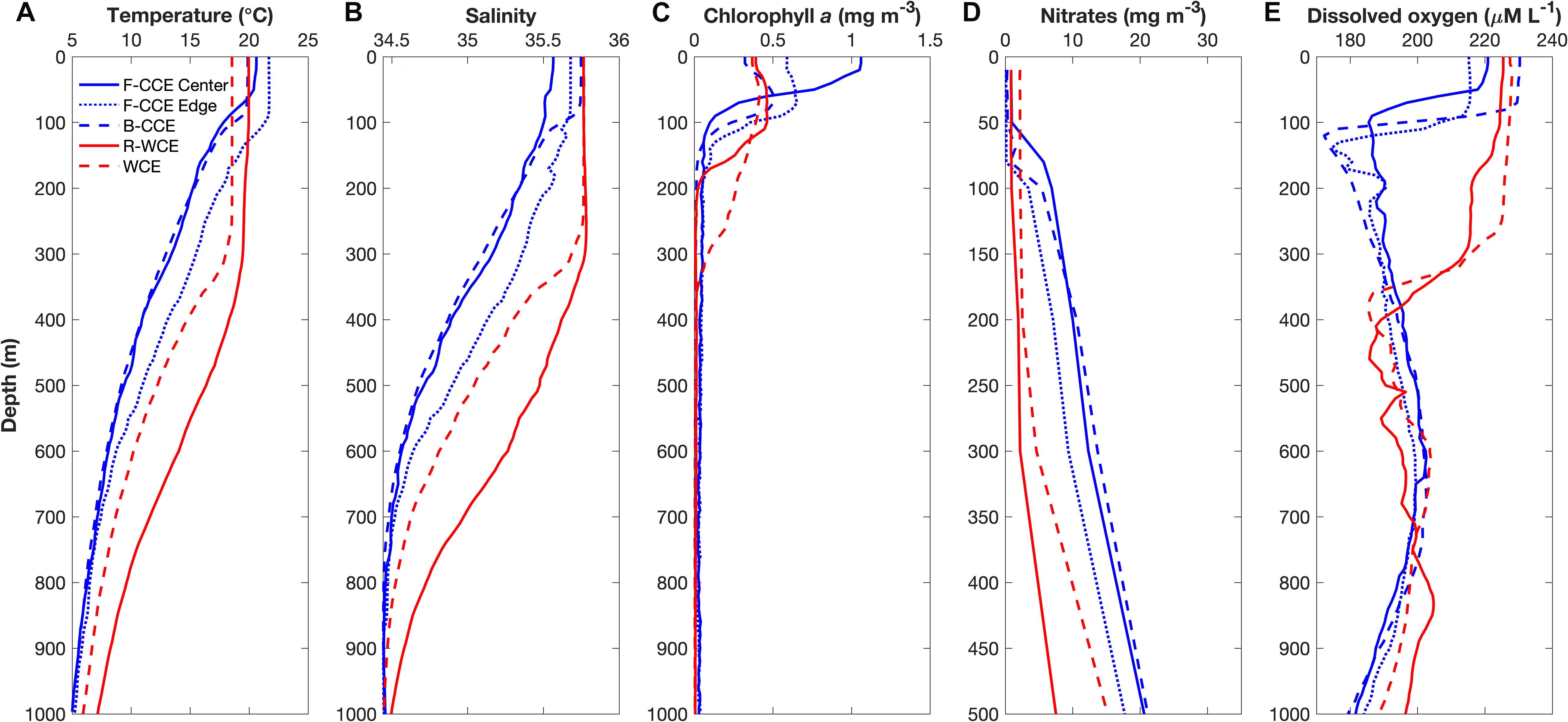
Figure 2. Depth profiles of (A) temperature (°C), (B) salinity, (C) chlorophyll a (mg m–3), (D) nitrates (mg m–3), and (E) dissolved oxygen (μM L–1) in the F-CCE Center (blue solid), F-CCE Edge (blue dotted), B-CCE (blue dashed), R-WCE (red solid), and WCE (red dashed).
The B-CCE was starting to decay, as evidenced from the rising sea-level anomaly (not shown; Ocean Current via IMOS2). It had a shallow mixed layer depth (MLD) (91 m; Figure 2A), low surface nutrients (Figure 2D), and low chlorophyll a, with a chlorophyll a max (0.51 mg m–3) occurring near the MLD (Figure 2C). Below the mixed layer, dissolved oxygen declined rapidly until ∼100 m, but did not reach hypoxic conditions (Figure 2E).
The R-WCE and WCE were both approximately 1–2 months old and formed from the EAC. Both the R-WCE (MLD, 236 m) and WCE (MLD, 322 m) were deeply mixed and characterized by saline, oligotrophic water (Figures 2A–C). Across all water masses, nutrient levels were the highest in surface waters (0–50 m) of the WCE (2.17 ± 0.02; F4,17 = 2073.45, p < 0.001), and both nutrients and chlorophyll a remained well mixed in the top 200 m of the WCE. Nutrient levels were low and well mixed in the R-WCE to 300 m. Prior to and during sampling, the complex R-WCE was entraining oligotrophic EAC water, resulting in a lower nutrient concentration, as was observed in the CTD profiles. Hence, it is difficult to observe the R-WCE from satellite SST and chlorophyll a (Figure 1). Dissolved oxygen remained high in the mixed layers of both the R-WCE and WCE, reaching minimums at 460 and 380 m, respectively (Figure 2E).
Mesozooplankton and Micronekton
Total Water Column Biomass
In 2015, mesozooplankton biomass in the F-CCE ranged from 1.2 to 2.3 mg C m–3. Our data met the assumptions of homogeneity of variance and normality (Supplementary Table S4). We detected no statistically significant difference in total water-column mesozooplankton biomass between the F-CCE Center and Edge (p = 0.41). Day and night mesozooplankton biomass was significantly different at the F-CCE Center (p = 0.007), while no difference was detected at the F-CCE Edge (p = 0.649) (Supplementary Table S5). Generally, biomass at both the F-CCE Center and Edge was higher at night (2.31 ± 0.09 and 1.68 ± 0.33 mg C m–3, respectively) than during the day (1.24 ± 0.007 and 1.41 ± 0.54 mg C m–3, respectively) (Figure 3).
FIGURE 3
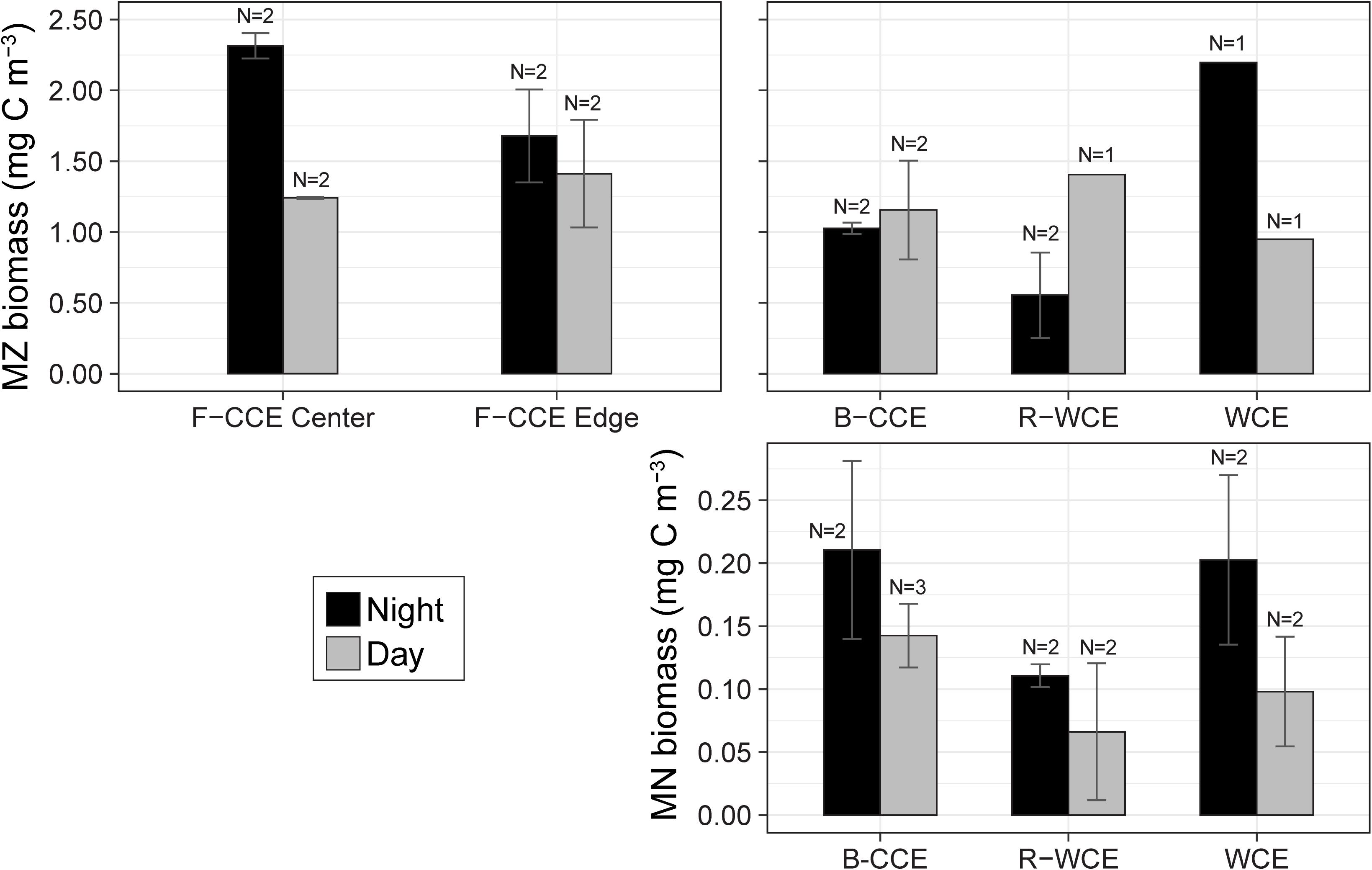
Figure 3. Total water column mean mesozooplankton (MZ; top) and micronekton (MN; bottom) biomass (mg C m–3) in the top 500 (MZ) and 1000 m (MN) during the night (black) and day (gray) at the F-CCE Center, F-CCE Edge, B-CCE, R-WCE, and WCE. Bars indicate ± standard error of the mean.
In 2017, the total water-column mesozooplankton biomass ranged from 0.55 to 2.2 mg C m–3. The mesozooplankton biomass in the B-CCE did not vary significantly between day and night (p = 0.77; Supplementary Table S7). Daytime biomass in the R-WCE was higher than nighttime, while the WCE showed the opposite trend with substantially higher biomass at night (Figure 3). We were unable to test these differences statistically due to lack of replication.
Mean micronekton biomass was consistently higher at night than during the day and ranged from 0.07 to 0.21 mg C m–3. However, day and night differences were not statistically significant in all three eddies (p > 0.32; Figure 3; Supplementary Table S5). This suggests that our sampling captured similar overall micronekton biomass during the day and night across all three eddies (see the section “Vertical Migration and Active Carbon Transport” for discussion of net avoidance). The majority of micronekton biomass (68–83%) was made up of myctophids (38–62%) and decapods (22–31%). Cephalopods (4–14%) and other fish (7–15%) were the next most dominant in terms of carbon biomass. All other groups contributed <5% to the total biomass (Table 2). Thus, we calculate migratory biomass and active carbon transport for all micronekton, and present only the results for myctophids and decapods in detail.
TABLE 2
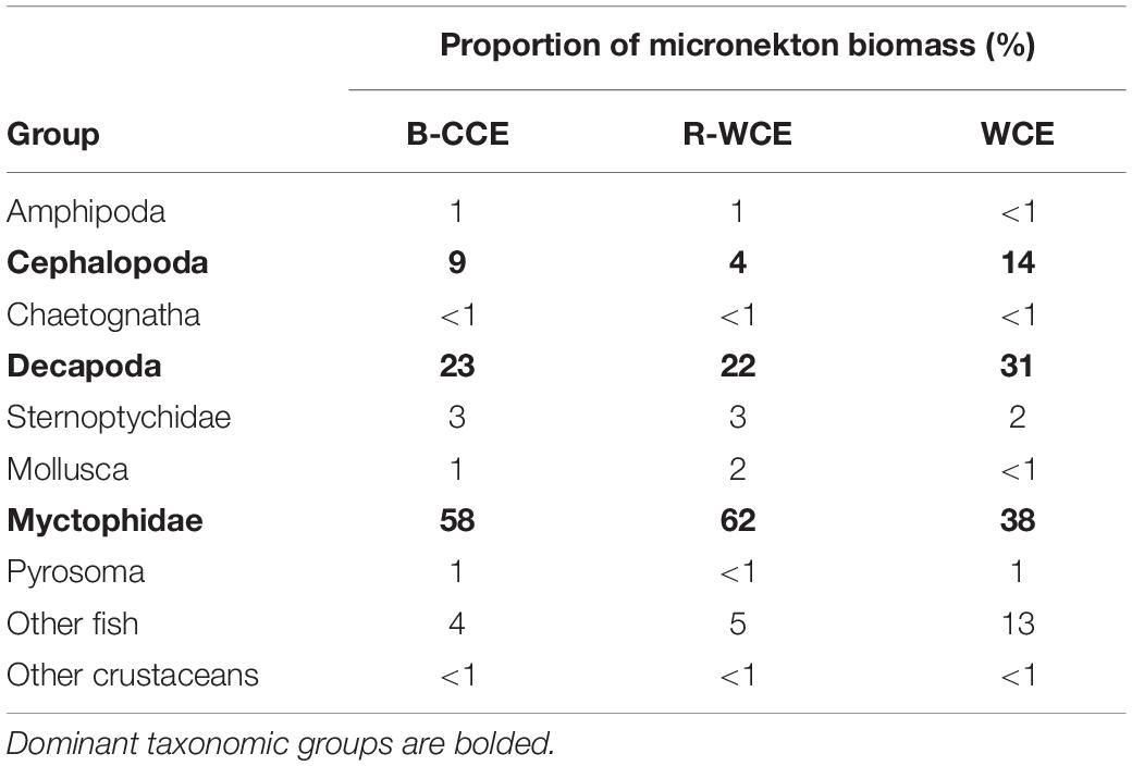
Table 2. Proportion of micronekton carbon biomass by major taxonomic group captured in the MIDOC.
Vertically Resolved Biomass
In 2015, mesozooplankton biomass (mean ± SE) in the top 100 m increased by >200% at night in the F-CCE Center (night = 15 ± 0.6 and day = 6 ± 0.05 mg C m–3) and increased by 50% in the F-CCE Edge (night = 9 ± 0.7 and day = 6 mg C m–3) (Figure 4). All other depth strata showed minimal changes between the day and night at the F-CCE Center and Edge (Figure 4), suggesting that mesozooplankton from below our maximum sampling depth (500 m) were migrating into the top 100 m of the water column at night.
FIGURE 4
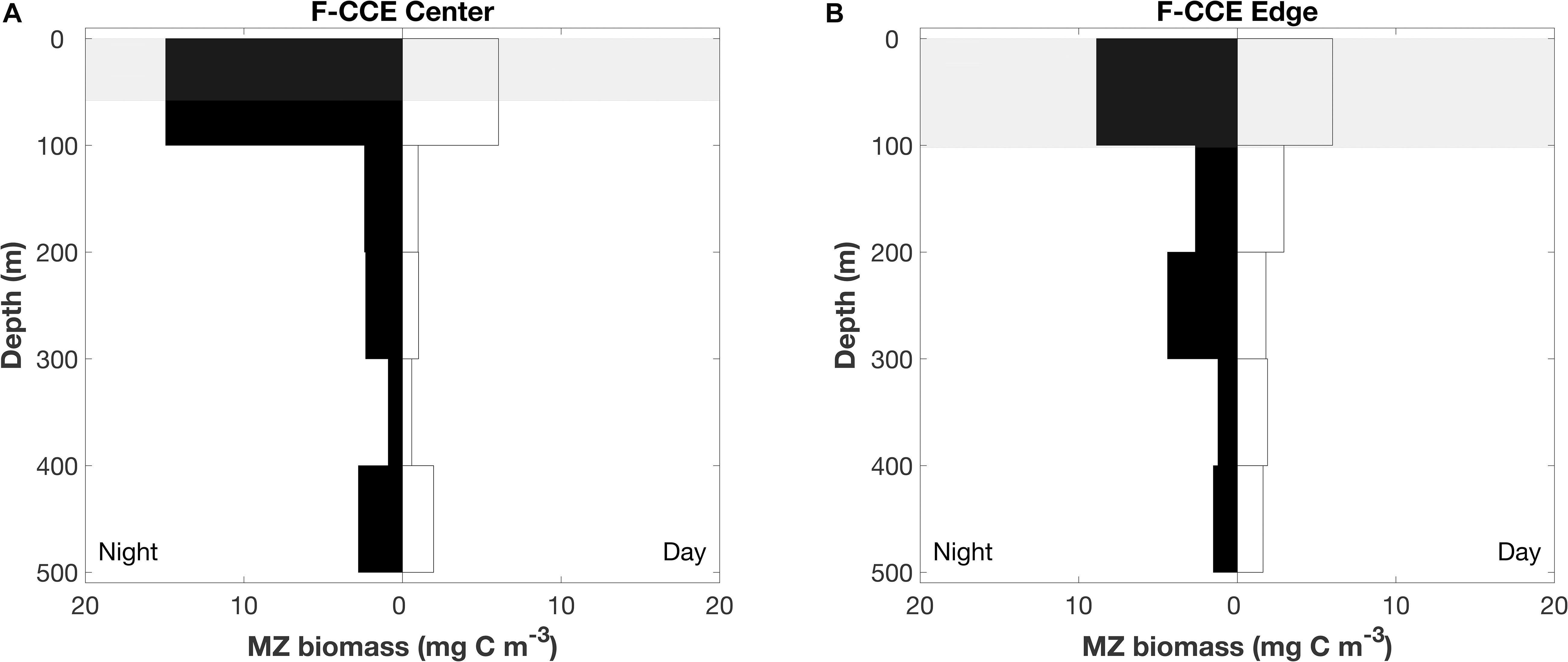
Figure 4. Depth profile of mesozooplankton at the (A) F-CCE Center and (B) F-CCE Edge. Nighttime profiles are left-hand panes, and daytime profiles are right-hand panes. Shaded gray areas represent mean (±SD) mixed layer depth.
In 2017, mesozooplankton biomass was highest at night in the top 100 m except for the R-WCE, which had higher biomass during the day in the 100 m depth stratum (Figure 5). Overall, mesozooplankton biomass in the top 100 m at night was at least three times greater in the WCE (134 mg C m–3) than in the B-CCE (44 ± 3 mg C m–3) and the R-WCE (38 mg C m–3) (Figure 5). During the day, biomass in the top 100 m decreased in the B-CCE (35 ± 6 mg C m–3) and the WCE (27 mg C m–3), while biomass in the R-WCE increased (62 mg C m–3). Biomass was generally higher in all other depth strata during the night except for the WCE 400–300 m depth stratum (Figure 5). Thus, mesozooplankton were performing DVM into the top 100 m at night in the B-CCE and the WCE, and reverse DVM into the top 100 m during the day in the R-WCE (Figure 5).
FIGURE 5
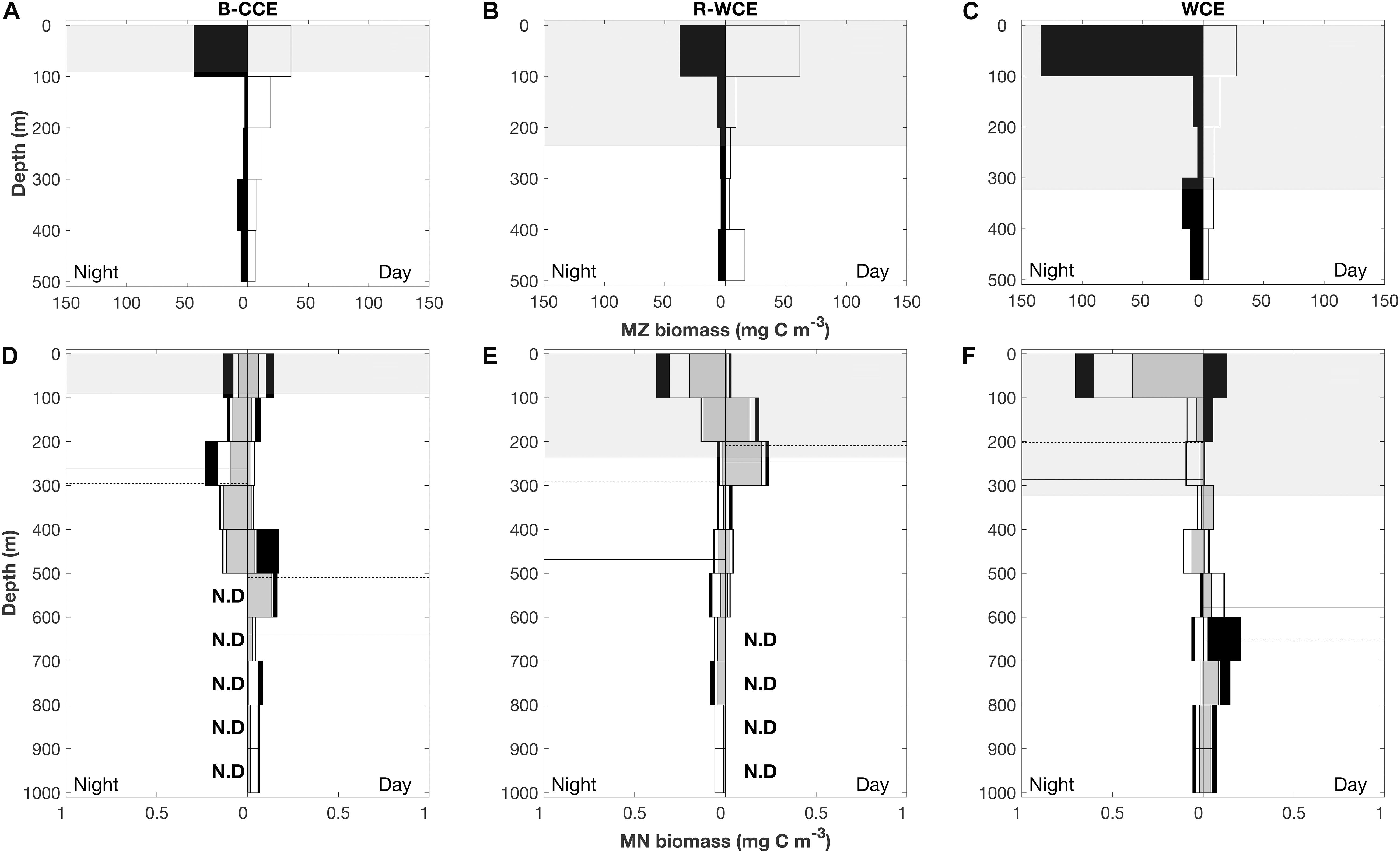
Figure 5. Depth profile of mesozooplankton (MZ; A–C) and micronekton (MN; D–F) in the B-CCE, R-WCE, and WCE. Micronekton biomass is split into myctophids (gray), decapods (white), and all other micronekton (black). Nighttime profiles are left-hand panes, and daytime profiles are right-hand panes. Dashed lines represent weighted mean depths for myctophids solid lines represent weighted mean depths for decapods. Shaded gray areas represent mean (±SD) mixed layer depth. N. D indicates no data.
Total micronekton biomass increased at night in the top 100 m in the R-WCE and the WCE, while remaining relatively constant in the B-CCE (Figure 5). Notable changes in the contribution of myctophids and decapods to total biomass in each depth stratum were observed during the day and night. In the B-CCE, myctophids and decapods were more prevalent >300m at night and <300 m during the day (Figure 5D), with decapods making up the majority of the migratory biomass (Table 3). The R-WCE showed a similar trend, although myctophid and decapods were more prevalent >200 m at night and <100 m during the day (Figure 5E), with myctophids made up the majority of the migratory biomass (Table 3). In the WCE, myctophids were prevalent in the top 100 m during both the day and night, yet biomass increased below 600 m during the day (Figure 5F), with decapods making up the majority of the migratory biomass (Table 3). A notable increase in decapod biomass in the top 100 m was observed at night in the WCE (Figure 5F).
TABLE 3
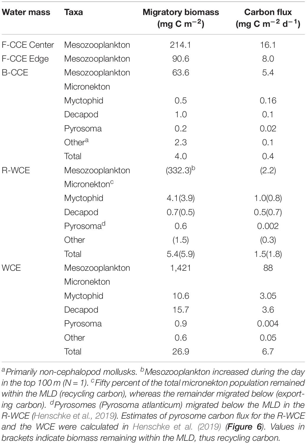
Table 3. Total migratory biomass (mg C m–2) and active carbon flux (mg C m–2) by mesozooplankton and micronekton for each water mass.
Overall, the WMD of myctophids and decapods became shallower at night in the B-CCE and the WCE (Figures 5D,F), indicating that the populations were undergoing DVM. Myctophids migrated from daytime WMDs of 497 and 652 m to nighttime WMDs of 296 and 202 m in the B-CCE and the WCE, respectively. Similarly, decapods migrated from daytime WMDs of 634 and 577 m to nighttime WMDs of 262 and 286 m in the B-CCE and the WCE. Total migratory biomass into the MLD was substantially higher in the WCE (262 μg C m–3 d–1) than in the B-CCE (50 μg C m–3 d–1). In the R-WCE, WMDs for myctophids and decapods were shallower during the day than at night (Figure 4). For myctophids, WMD was 205 m during the day and 292 m at night and for decapods 237 m during the day and 469 m at night. Further, 44 and 42% of the myctophid and decapod population were remaining within the MLD during the day (Figure 4), while the rest were migrating below the MLD.
Active Carbon Transport
Total downward carbon flux by mesozooplankton and micronekton varied across water masses. In 2015, mesozooplankton downward carbon export at the F-CCE Center (16.1 mg C m–2 d–1) was double that at the F-CCE Edge (8.0 mg C m–2 d–1) (Table 3).
In 2017, total migratory mesozooplankton and micronekton biomass was highest in the WCE (Table 3). Similarly, total mesozooplankton and micronekton downward carbon flux below the MLD was substantially higher in the WCE (88 and 6.7 mg C m–2 d–1, respectively) than in the B-CCE (5.4 and 0.4 mg C m–2 d–1, respectively) (Table 3). Mesozooplankton migrated within the MLD in the R-WCE, recycling carbon in the top 200 m of the water column (2.2 mg C m–2 d–1) (Table 3). Additionally, only 56 and 58% of the myctophid and decapod biomass were migrating below the MLD, while all other micronekton remained within the MLD during the day and night (Figure 5). Therefore, 50% of the total biomass and 51% of the active carbon flux in R-WCE were being exported below the MLD during DVM, equating to 1.5 mg C m–2 d–1 (Table 3).
Overall, respiratory and mortality flux contributed the most to downward carbon transport in all three water masses (Table 4). We found that mortality flux varied substantially depending on the model approach (Table 5). When estimated from growth, mortality was greater for mesozooplankton in the F-CCE Center and Edge, and lower for mesozooplankton in the B-CCE and WCE (Table 5). In contrast, both approaches yielded similar results for micronekton, though estimates derived from growth were generally more conservative.
TABLE 4
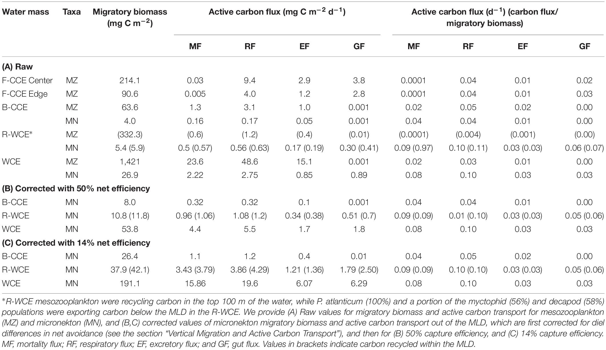
Table 4. Migratory micronekton biomass (mg C m–2) and active carbon fluxes (expressed in mg C m–2 d–1 and d–1) out of the MLD in the F-CCE Center, Edge, B-CCE, and WCE, and carbon recycling in the R-WCE.
TABLE 5
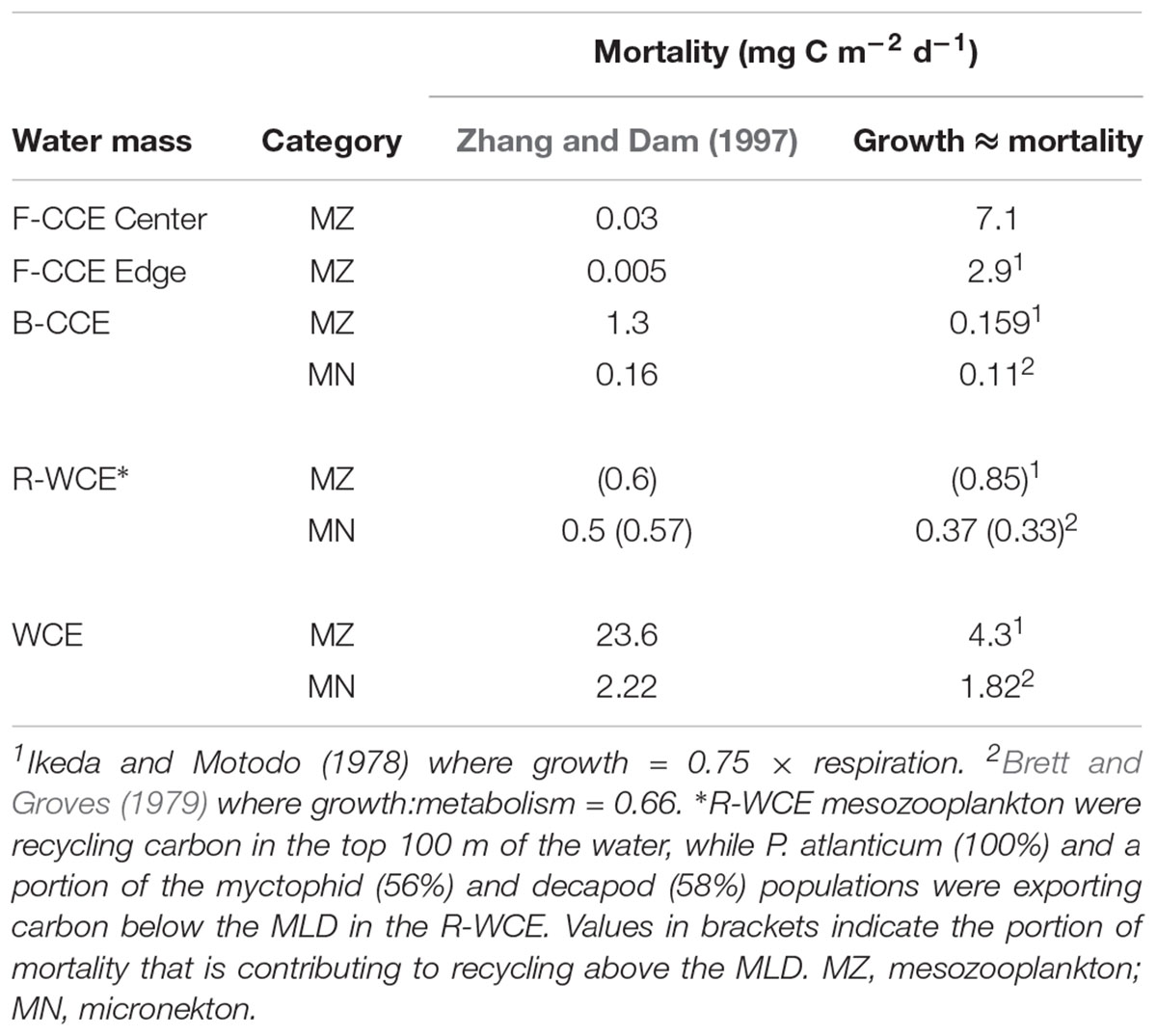
Table 5. Comparison of two different approaches to estimate mortality of mesozooplankton and micronekton: (1) Zhang and Dam (1997) isometric approach based on Peterson and Wroblewski (1984), and (2) assuming the system is under steady-state and mortality is approximately equivalent to growth, various growth rate equations have been applied.
Although mesozooplankton contributed more to overall downward carbon transport in each water mass, when scaled based on migratory biomass (i.e., carbon flux/migratory biomass for each group) micronekton ultimately contributed more to downward carbon transport (Table 4). Of all micronekton groups, myctophids and decapods contributed the most to carbon flux in all three water masses (Table 3). Specifically, myctophids contributed more in the B-CCE and WCE, while decapods contributed more in the R-WCE when scaled based on migratory biomass (Table 4).
Discussion
This study quantifies mesozooplankton and micronekton active carbon flux in contrasting eddies. Although differences in mesozooplankton and micronekton composition in warm- and cold-core eddies have previously been assessed (e.g., The Ring Group, 1981; Goldthwait and Steinberg, 2008; Eden et al., 2009), their contribution to active carbon flux within and across eddies remains poorly understood (e.g., Goldthwait and Steinberg, 2008; Landry et al., 2008). Despite similarities in total water column biomass, we observed notable differences in mesozooplankton and micronekton migratory biomass and their contribution to carbon export across eddies. Mesozooplankton and micronekton were contributing to downward carbon export below the MLD in the F-CCE Center and Edge, B-CCE, and WCE, and recycling carbon in the R-WCE.
Mesozooplankton and Micronekton Total Water Column Biomass
Eddies form partially isolated and distinct biological communities which can be transported large distances (Mackas and Galbraith, 2002; Batten and Crawford, 2005; Eden et al., 2009; Suthers et al., 2011; Condie and Condie, 2016). They can aggregate micronekton populations due to bottom-up effects intensifying food-web interactions. This aggregation occurs primarily at the eddy periphery rather than center where production is highest (Sabarros et al., 2009; Drazen et al., 2011). We observed minimal differences in mesozooplankton total water column biomass between the F-CCE Center and Edge. This is contrary to most studies which report elevated mesozooplankton abundance and biomass at eddy centers (e.g., Mackas et al., 2005; Landry et al., 2008; Everett et al., 2011). However, differences between day and night total water-column biomass were more pronounced at the F-CCE Center than the F-CCE Edge, suggesting intensified DVM in eddy centers (Eden et al., 2009). As our study only sampled mesozooplankton down to 500 m in 2015, it is possible that a portion of the nighttime biomass was originating from below our sampling depth (see the section “Vertical Migration and Active Carbon Transport”).
Factors influencing the biological community within eddies include eddy age, size, phase (Eden et al., 2009), retention time (Condie and Condie, 2016), and the characteristics of the source waters (Olson, 1991; Strzelecki et al., 2007; Mullaney and Suthers, 2013). In this study, mesozooplankton and micronekton total water column biomass was similar in cold- and warm-core eddies. This is consistent with past studies reporting similar zooplankton biomass in contrasting eddies, despite vast differences in eddy type and chlorophyll a concentration (Goldthwait and Steinberg, 2008; Eden et al., 2009). These studies suggest that the two eddy types may be equally productive depending on conditions of their formation (Goldthwait and Steinberg, 2008; Eden et al., 2009; Dufois et al., 2016). In our sampling region, cold-core eddies are generally more productive due to upwelling of nutrient rich waters fueling primary production (Govoni et al., 2010; Everett et al., 2012); hence, we expected to see higher biomass of mesozooplankton and micronekton in the B-CCE. During sampling, however, the B-CCE was in the decay phase, as the sea level anomaly was subsiding, and surface nutrient and chlorophyll a were low. Therefore, differences in biota that may have existed at the eddy formation could have been undetectable at the time of sampling (The Ring Group, 1981; Eden et al., 2009). Indeed, all three eddies sampled in 2017 had similar chlorophyll a in the top 100 m layer. Considering the decaying productivity in the B-CCE, the similarities in total water column biomass across eddy types in 2017 could be attributed to their similar source waters (i.e., Coral Sea and EAC; Jyothibabu et al., 2015).
Vertical Migration and Active Carbon Transport
Past studies have reported intensification of DVM within mesoscale eddies (Yebra et al., 2005; Goldthwait and Steinberg, 2008; Landry et al., 2008; Eden et al., 2009). However, only a few studies have attempted to quantify carbon export in eddies (e.g., Yebra et al., 2005; Landry et al., 2008). To our knowledge, this study represents the first assessment of active carbon flux incorporating both mesozooplankton and micronekton across contrasting eddies in the southwest Pacific Ocean.
The magnitude of day and night differences in total water column biomass (see the section “Mesozooplankton and Micronekton Total Water Column Biomass”) as well as total nighttime biomass in the top 100 m were both substantially higher at the F-CCE Center than Edge, suggesting intensified mesozooplankton DVM at eddy centers (Goldthwait and Steinberg, 2008; Landry et al., 2008; Eden et al., 2009). Chlorophyll a at the F-CCE Center was more than double that of the F-CCE Edge. Thus, we attribute these differences in DVM behavior and carbon export at the F-CCE Center versus Edge to higher food availability, as zooplankton may decrease the extent of their vertical migrations when food availability is low (Huntley and Brooks, 1982; Lampert, 1989). Mesozooplankton biomass in the top 100 m increased at night in the B-CCE and the WCE, and during the day in the R-WCE. The latter points to reverse DVM in the R-WCE, although only one daytime replicate was available for the R-WCE. As chlorophyll a was similar in all three eddies these differences in DVMs were not solely driven by the food availability. In the B-CCE and the R-WCE mesozooplankton, biomass in the top 100 m were substantially lower than in the WCE indicating lower food availability prior to sampling, assuming all three eddies had similar source waters. Mesozooplankton exhibit DVM behavior as a means to improve metabolism (McLaren, 1963; McLaren, 1974; Enright, 1977; Iwasa, 1982; Hernández-León et al., 2010) and reduce exposure to visual predation (Iwasa, 1982; Hays et al., 1997). Temperature decreased more rapidly below the MLD in the B-CCE than in the R-WCE, indicating that the benefits of DVM related to improved metabolism were likely higher in the former. Further, the MLD was much shallower in the B-CCE (91 m) than in the R-WCE (236 m), suggesting that mesozooplankton may have had lower metabolic costs in getting to a metabolically advantageous depth in the B-CCE. It is thus possible that mesozooplankton in the R-WCE were undergoing reverse DVM primarily to reduce exposure to visual predation by micronekton, which were exhibiting concurrent normal DVM within the MLD (Ohman, 1986). However, it should be noted that no mesozooplankton replicates were available during the day in the R-WCE. Only 50% of the micronekton population migrated below the MLD during the day in the R-WCE. The reduced DVM by micronekton in the R-WCE is likely explained by relatively low food availability (i.e., chlorophyll a and mesozooplankton biomass) and reduced metabolic benefits, as temperature remained relatively high down to 400 m, after which it slowly decreased.
Differences in DVM and MLD between eddies led to considerable differences in the magnitude and depth of carbon export across water types. The shallower MLD in cold-core eddies than in warm-core eddies (Waite et al., 2019) suggests that organisms must migrate deeper to effectively contribute to carbon export in warm-core eddies. In this study, mesozooplankton and micronekton were vertically migrating below the MLD, thus contributing to downward active carbon flux in the F-CCE Center and Edge, B-CCE and WCE. Our results support past studies reporting higher active carbon fluxes by mesozooplankton at eddy centers (Yebra et al., 2005; Landry et al., 2008), as export at the F-CCE Center (16.1 mg C m–2 d–1) was more double that of the F-CCE Edge (8.0 mg C m–2 d–1). In the Canary Islands, Yebra et al. (2005) assessed respiratory and gut flux of mesozooplankton in a WCE, reporting similarly elevated respiratory carbon fluxes at the eddy center compared to the eddy edge and minimal differences in gut flux relative to total biomass. We did not sample the eddy edges in 2017. In the B-CCE and the WCE, mesozooplankton contributed 5.4 and 88 mg C m–2 d–1 to downward active carbon transport, respectively. In the R-WCE mesozooplankton biomass remained unchanged during the day and night, suggesting that they were recycling carbon (2.2 mg C m–2 d–1) within the MLD. Our estimates of mesozooplankton respiratory and mortality flux (9.97–23.53 mg C m–2 d–1) were similar to Hidaka et al. (2001) in the western equatorial Pacific at the B-CCE, F-CCE Center and Edge, while the WCE was an order of magnitude higher. The higher carbon export in the WCE was supported by substantially higher mesozooplankton migratory biomass.
In the B-CCE, R-WCE, and WCE micronekton contributed 0.4, 1.5, and 6.7 mg C m–2 d–1 to downward carbon export. Only 50% of the micronekton population was contributing to downward carbon transport in the R-WCE, while the remainder was recycling carbon within the MLD. It is well documented that nets may under sample micronekton by an order of magnitude due to avoidance (Koslow et al., 1997; Kaardvedt et al., 2012). This avoidance reportedly exhibits diel variation, with greater net avoidance during the day than at night (e.g., Wiebe et al., 1982), which may lead to overestimated migratory and active carbon fluxes (Angel and Pugh, 2000). Therefore, we first re-scaled the biomass of our highly migratory groups (i.e., myctophids and decapods), such that total water column biomass during the day and night were equivalent, and then re-ran our model. This only corrects for the discrepancy between day and night net avoidance (Supplementary Table S1). Our micronekton biomass was an order of magnitude lower than mesozooplankton biomass; based on ecological theory, we would expect to see equal biomass within equally logarithmic size bins (Sheldon et al., 1972; Blanchard et al., 2017). This discrepancy could be due to net efficiency, which typically ranges from 4 to 14% for micronekton net sampling (Gjøsaeter, 1984; May and Blaber, 1989; Koslow et al., 1997; Davison, 2011; Kaardvedt et al., 2012). To correct for this, we applied an additional correction of 14% from Koslow et al. (1997) that was calculated for a similar micronekton community in southeastern Australia. While this is the best available correction for our data, it should be noted that our sampling approach differs slightly from that of Koslow et al. (1997) in terms of tow speed (1 vs. 1.5 m/s), net dimension (157.5 vs. 105 m2), and mesh size (200 mm tapering to 10 mm at the codend vs. 100 mm tapering to 10 mm at the codend), which may influence the overall net efficiency. Thus, we also apply a more conservative correction for net efficiency of 50% for comparison with other studies in the literature (i.e., Hernández-León et al., 2019). All conversions are shown in Supplementary Table S8. Similar to Hernández-León et al. (2019), we found that different net efficiencies led to vast differences in overall downward carbon export (Table 4). We provide values for both efficiencies (Table 4), but estimate and discuss active carbon transport going forward using the more conservative net efficiency of 50% (Figure 6).
FIGURE 6
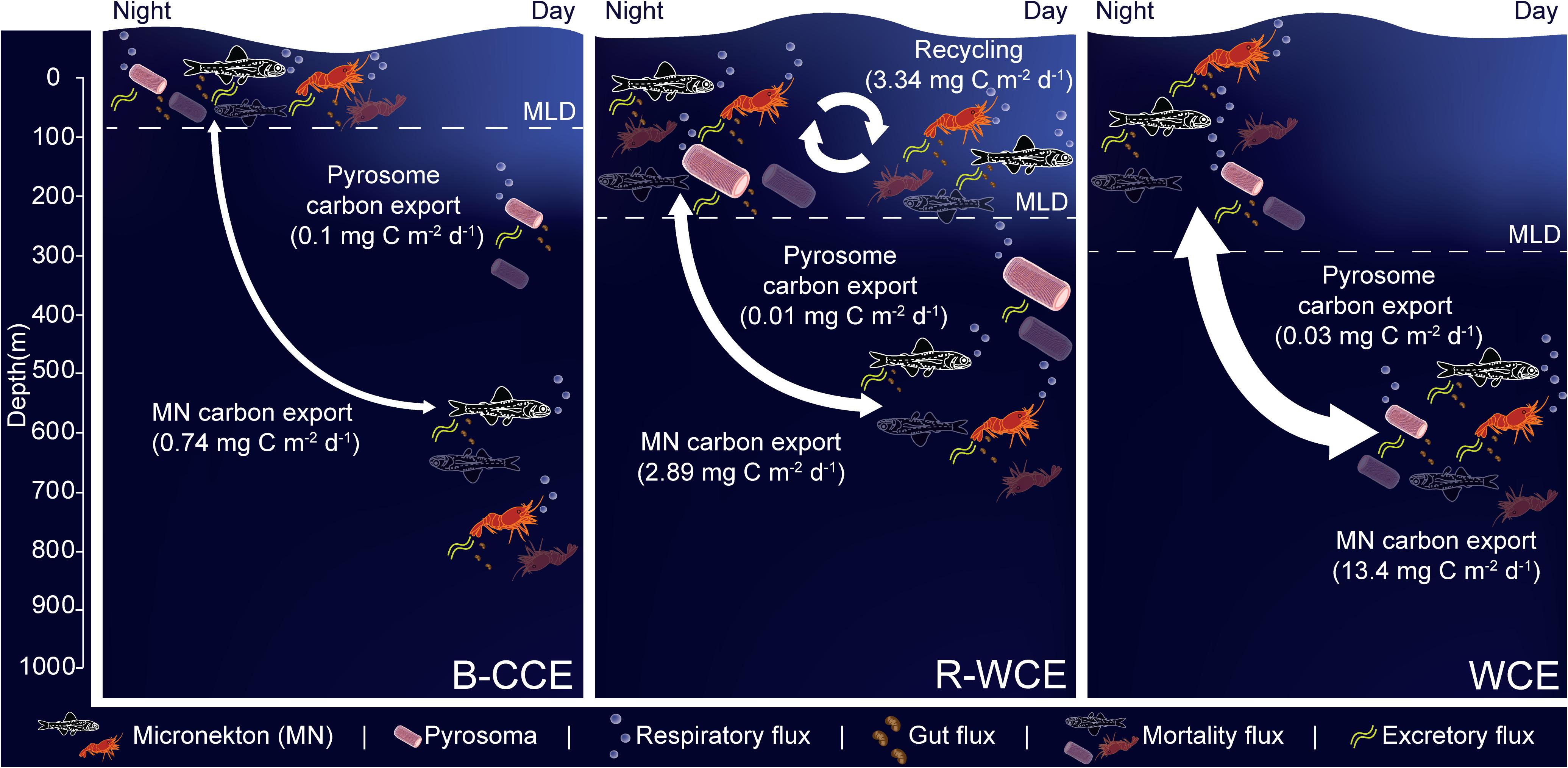
Figure 6. Micronekton active carbon flux and depth of vertical migration in the B-CCE, R-WCE, and WCE. Dashed line represents the mixed layer depth (MLD). Estimates of pyrosome (Pyrosoma atlanticum) active carbon for the R-WCE and WCE were calculated in Henschke et al. (2019). Values reported assume 50% net efficiency (Table 4). MF, mortality flux; GF, gut flux; RF, respiratory flux; and EF, excretory flux.
Myctophids and decapods contributed the most to micronekton downward carbon flux in all three eddies. Except for Henschke et al. (2019), no other study had focused on active carbon transport of micronekton within eddies making it difficult to compare our results with previous studies. Estimates of active carbon transport by decapods and myctophids vary substantially spatially and temporally (Hidaka et al., 2001; Davison et al., 2013; Schukat et al., 2013; Ariza et al., 2015; Pakhomov et al., 2018; Gorgues et al., 2019), thus caution must be taken when comparing estimates. When corrected with a net efficiency of 50%, and expressed as d–1 (downward carbon export/migratory biomass; see Table 4) our estimates were comparable to past studies of Hidaka et al. (2001) in western equatorial Pacific (14% net efficiency correction for micronekton respiratory and gut flux: 15.2–29.9 mg C m–2 d–1), Ariza et al. (2015) near the Canary Islands (micronekton respiratory flux: 2.9 mg C m–2 d–1) and Angel and Pugh (2000) in the northeast Atlantic (12.5–58 mg C m–2 d–1). Davison et al. (2013) assessed fish-mediated export in the highly productive California Current, reporting values substantially higher than those of the WCE. However, a direct comparison is difficult without knowing the precise size range of fishes used in Davison et al. (2013). Pyrosoma atlanticum contributed minimally to active carbon flux (<1–7% of total flux in the B-CCE, WCE, and R-WCE; Figure 6). Although when biomass is high pyrosomes may export up to 11 mg C m–2 d–1 (Henschke et al., 2019). Our study demonstrates that myctophids and decapods are equally important as micronekton in their contribution to downward carbon transport. In some cases, the contribution of decapods to downward carbon transport may even exceed that of myctophids in mesoscale eddies. Hernández-León et al. (2019) reported that decapods coincided with sharp oxygen minimum zones (OMZs) in the subtropical Atlantic Ocean. In our study, the B-CCE exhibited a sharp decline in oxygen at the base of the MLD (∼100 m), in this case the migratory biomass of decapods exceeded that of myctophids. This finding supports Hernández-León et al. (2019), as decapods are known to be more tolerant of low oxygen concentrations (Childress, 1975). Thus, it is important to consider all groups, including highly variable and/or patchy species when making active flux estimates.
Contrary to Hidaka et al. (2001), we found that mesozooplankton contributed more to downward carbon export than micronekton in the B-CCE and WCE, while only micronekton were contributing to export in the R-WCE. This difference was primarily driven by the higher metabolic rates, and thus respiratory flux, of mesozooplankton when compared to micronekton (Ikeda, 1985, 2016). However, our sampling was concentrated in eddy centers, so it is possible that we missed the portion of micronekton that is thought to aggregate at eddy peripheries (Sabarros et al., 2009; Drazen et al., 2011). Our mesozooplankton and micronekton showed similar trends, with the highest export occurring in the WCE, followed by the B-CCE and R-WCE.
Although we only collected mesozooplankton at the F-CCE Center and Edge in 2015, we would expect this trend to hold true as Hernández-León et al. (2019) reported a significant positive relationship between zooplankton and micronekton total active flux. Our findings suggest that mesoscale eddies can act as important carbon sinks.
Uncertainty and Limitations
A number of empirical equations from the literature were applied to estimate respiration, DOC excretion, mortality, and gut flux. The uncertainty associated with the models may indeed plague such estimates. Respiration was estimated using empirical allometric relationships dependent on carbon weight and in situ temperature from the literature (Ikeda, 2013b, 2014, 2016; Henschke et al., 2019). For all relationships used, temperature and weight explained >86% of the variation in oxygen uptake, suggesting minimal uncertainty with the models. DOC excretion was estimated based on excretory rates of several different taxonomic groups, including shrimp, euphausiids, copepods, amphipods, and polychaetes compiled in Steinberg et al. (2000). The study found that excretory flux was consistently ∼31% of respiratory flux across all taxonomic groups. Similar to respiration, DOC excretion rates were dependent on temperature and organism dry weight (Steinberg et al., 2000). The error margin associated with excretory flux is considered minor. In addition, this flux contributed minimally to the total carbon export budget. For estimates of gut flux, we compiled values of ISF and GPT from the literature for various taxa (Supplementary Table S7). To be conservative, where multiple values were available, we used the shortest values in our model. All values were corrected for differences in temperature and applied on an individual basis. Uncertainty may arise with gut flux estimates as none of these values take into consideration organism size, feeding history, overall stomach fullness, which may lead to variable GPTs. We assumed that organisms were continuously feeding at night in the mixed layer. This may lead to some overestimation as they may conduct intermittent feeding that can be difficult to quantify. However, while the contribution of gut flux to active carbon transport can be great, in this study it was minimal in all water masses. Most active carbon flux studies choose not to include mortality flux as it is highly variable and dependent on food availability, environmental, and predator abundance.
Mortality was calculated using the Zhang and Dam (1997) adaptation of Peterson and Wroblewski (1984) size-dependent mortality rate model for fishes ranging from 0.1 mg (eggs) to 1000 g (adults) dry weight. This model spans a wide variety of species and sizes of organisms and may lead to overestimation, particularly at the extremes of the mass range. This study simply represents a starting point, as stomiid predation on mesopelagic fish alone is estimated to range from 58 to 230% (Clarke, 1982; Hopkins et al., 1996; Davison et al., 2013). Thus, we provide a direct comparison with our values and the approach taken in Hernández-León et al. (2019), which assumes that the system is in steady-state and thus mortality is approximately equivalent to growth (Table 5). Our results demonstrate that vastly different estimates of mortality flux can be obtained by the two different approaches, and that one is not consistently more conservative than the other. Therefore, we recommend that future studies focus on refining the uncertainty associated with estimating gut and mortality flux.
Mesozooplankton were sampled using a MOCNESS with a 500-μm mesh. Therefore, smaller mesozooplankton (200–500 μm) were not captured leading to underestimates in total mesozooplankton abundance and biomass, particularly in the spring (i.e., 2017) when nauplii and copepodites numbers are high (Kimmerer and McKinnon, 1987).
The largest uncertainty pertains to micronekton sampling. We were unable to account for escapement and herding. Nets with tapering mesh often lead to underestimates in micronekton biomass, as small weak swimming micronekton often escape through the coarse mesh at the mouth of the net, while large strong swimming micronekton are “herded” toward the back of the net where the mesh size is small enough for retention (Lee et al., 1996; Koslow et al., 1997; Voronina and Pakhomov, 1998). A degree of error pertaining to the calculation of volume filtered for the MIDOC also exists. This value is calculated based on the spread and height of the midwater trawl doors, which can vary throughout a tow. We used the average spread and height of the trawl to calculate volume filtered, but at present have no way of correcting for deviations that can arise due to currents and winds inflicted on the net as well as animal herding by the net (Voronina and Pakhomov, 1998; Heino et al., 2011). Thus, we assume our uncorrected estimates of micronekton biomass to be conservative and likely on the lower end.
Finally, past studies have reported seasonal variation in the migratory behavior of mesopelagic fishes (e.g., Staby and Aksnes, 2011; Urmy et al., 2012), suggesting that the intensity (i.e., depth) of DVM is suppressed during the spring for some mesopelagic fishes. As our sampling was conducted during the winter of 2017 and the spring of 2015, micronekton were likely exhibiting less intense DVM, and thus contributing less to downward carbon export.
Conclusion
We assessed the vertical distribution and carbon export by mesozooplankton and micronekton in contrasting eddies. The magnitude and depth of DVM varied across water masses. Mesozooplankton exhibited intensified DVM and carbon export at the F-CCE Center in comparison to the edge. We observed similar total water column mesozooplankton and micronekton biomass in the B-CCE, R-WCE, and WCE, likely attributable to their similar source waters. However, notable differences in carbon export across eddies were observed. Generally, cold-core eddies had shallower MLD than warm-core eddies, suggesting that in order to contribute to carbon export (i.e., transport below the MLD) organisms had to migrate deeper in warm-core eddies. In the R-WCE, the MLD was deeper and temperatures were higher, suggesting that mesozooplankton were undergoing reverse DVM primarily to reduce exposure to visual predation as the metabolic advantages of DVM were reduced. Mesozooplankton contributed more to downward carbon export than micronekton in the B-CCE and WCE, and only micronekton were contributing to export in the R-WCE. Differences in carbon export appear to depend on food availability, temperature, time spent migrating, and MLD. Our findings suggest that under certain conditions mesoscale eddies can act as important carbon sinks.
Data Availability Statement
The raw datasets generated for this study are included in the article/Supplementary Material. Additional data will be provided on request.
Ethics Statement
The animal study was reviewed and approved by the Animal Care and Ethics Committee (ACEC) of the University of New South Wales.
Author Contributions
LK and NH conducted the data analysis and wrote the first draft of the manuscript. LK, NH, EP, and IS participated in the data collection and sample processing. IS, JE, and EP contributed to design and interpretation of results. All authors contributed to writing, revising, and approving the submitted version of the manuscript.
Funding
This work was partially funded by the Australian Research Council Discovery Projects scheme (DP140101340 and DP150102656), and a Natural Sciences and Engineering Research Council of Canada (NSERC) Discovery Grant (funding reference number RGPN-2014-05107). LK and NH were funded by the University of British Columbia funding to EP. The voyages (IN2015v03 and IN2017v04) were supported by ship-time grants to IS and JE from the CSIRO Marine National Facility.
Conflict of Interest
The authors declare that the research was conducted in the absence of any commercial or financial relationships that could be construed as a potential conflict of interest.
Acknowledgments
We would like to thank the CSIRO Marine National Facility (MNF) for its support in the form of sea time on the R/V Investigator, support personnel, scientific equipment, and data management. Finally, we would like to thank our fellow researchers who assisted in collecting samples in June 2015 and September 2017. Satellite data were sourced from the Integrated Marine Observing System (IMOS).
Supplementary Material
The Supplementary Material for this article can be found online at: https://www.frontiersin.org/articles/10.3389/fmars.2019.00825/full#supplementary-material
TABLE S1 | Number of samples performed at each location.
TABLE S2 | Presence/absence species list for MIDOC catches, where 1 = present and 0 = absent in the B-CCE, R-WCE, and WCE in September 2017.
TABLE S3 | Length to weight relationships used to calculate carbon weight (CW; in mg) for micronekton captured in the MIDOC. Lengths are reported as either total length (TL) or standard length (SL) in millimeters.
TABLE S4 | Testing the assumptions of ANOVA. The results for Bartlett’s test of homogeneity of variance and Shapiro-Wilk’s test for normality for total water column mesozooplankton and micronekton.
TABLE S5 | Results of ANOVA comparing day and night total water column mesozooplankton (EZ net) and micronekton (MIDOC) biomass captured in the F-CCE Center, F-CCE Edge, B-CCE, R-WCE, and WCE.
TABLE S6 | Regression equations used to calculate respiratory oxygen uptake (RO; μL O2.ind.-1 h-1), where DW is individual dry weight (mg), WW is individual wet weight (mg), T is temperature (°C), and D is depth (m).
TABLE S7 | Values of ISF (% of total body weight) and gut passage time (GPT; h) used to calculate active carbon transport. Where values were not available for specific species of fish the average ISF and GPT for mesopelagic fish were applied. Only organisms that were undergoing DVM are included. Where DW = dry weight (mg), CW = carbon weight (mg), T = temperature (°C), and FP = daily fecal pellet production.
TABLE S8 | Day/night avoidance variability correction and overall net avoidance calculation for migratory micronekton carbon fluxes (mg C m-2 d-1) out of the MLD in the B-CCE and WCE, and carbon recycling (values in brackets) in the R-WCE. Micronekton biomass is first corrected for diel differences in net avoidance (see the section “Vertical Migration and Active Carbon Transport”), and then for overall micronekton net avoidance assuming a net efficiency of 14% (Koslow et al., 1997). MF = mortality flux, RF = respiratory flux, EF = excretory flux, and GF = gut flux.
DATA SHEET S1 | Raw data.
Footnotes
References
Andersen, K. H., Berge, T., Gonçalves, R. J., Hartvig, M., Heuschele, J., Hylander, S., et al. (2016). Characteristic sizes of life in the oceans, from bacteria to whales. Ann. Rev. Mar. Sci. 8, 217–241. doi: 10.1146/annurev-marine-122414-034144
Angel, M. V., and Pugh, P. R. (2000). Quantification of diel vertical migration by micronektonic taxa in the northeast Atlantic. Hydrobiologia 440, 161–179. doi: 10.1023/A:1004115010030
Ariza, A., Garijo, J. C., Landeira, J. M., Bordes, F., and Hernández-León, S. (2015). Migrant biomass and respiratory carbon flux by zooplankton and micronekton in the subtropical northeast Atlantic Ocean (Canary Islands). Prog. Oceanogr. 134, 330–342. doi: 10.1016/j.pocean.2015.03.003
Baird, R. C., Hopkins, T. L., Wilson, D. F., and Bay, Y. (1975). Diet and feeding chronology of Diaphus taaningi (Myctophidae) in the Cariaco Trench. Am. Soc. Ichthyol. Herpetol. 1975, 356–365.
Batten, S. D., and Crawford, W. R. (2005). The influence of coastal origin eddies on oceanic plankton distributions in the eastern Gulf of Alaska. Deep. Res. Part II Top. Stud. Oceanogr. 52, 991–1009. doi: 10.1016/j.dsr2.2005.02.009
Blanchard, J. L., Heneghan, R. F., Everett, J. D., Trebilco, R., and Richardson, A. J. (2017). From bacteria to whales: using functional size spectra to model marine ecosystems. Trends Ecol. Evol. 32, 174–186. doi: 10.1016/j.tree.2016.12.003
Cetina-Heredia, P., Roughan, M., van Sebille, E., and Coleman, M. A. (2014). Long-term trends in the East Australian current separation latitude and eddy driven transport. J. Geophys. Res. Ocean. 119, 4351–4366. doi: 10.1002/2014JC010192.Received
Chenillat, F., Franks, P. J. S., Capet, X., Rivière, P., Grima, N., Blanke, B., et al. (2018). Eddy properties in the Southern California current system. Ocean Dyn. 68, 761–777. doi: 10.1007/s10236-018-1158-4
Childress, J. J. (1975). The respiratory rates of midwater crustaceans as a function of depth of occurrence and relation to the oxygen minimum layer off Southern California. Comp. Biochem. Physiol. A. Comp. Physiol. 50, 787–799. doi: 10.1016/0300-9629(75)90146-2
Choy, C. A., Popp, B. N., Hannides, C. C. S., and Drazen, J. C. (2015). Trophic structure and food resources of epipelagic and mesopelagic fishes in the north pacific subtropical Gyre ecosystem inferred from nitrogen isotopic compositions. Limnol. Oceanogr. 60, 1156–1171. doi: 10.1002/lno.10085
Clarke, T. A. (1982). Feeding habits of stomiatoid fishes from Hawaiian waters. Fish. Bull. 80, 287–304.
Condie, S., and Condie, R. (2016). Retention of plankton within ocean eddies. Glob. Ecol. Biogeogr. 25, 1264–1277. doi: 10.1111/geb.12485
Crabtree, R. E. (1995). Chemical composition and energy content of deep-sea demersal fishes from tropical and temperate regions of the western North Atlantic. Bull. Mar. Sci. 56, 434–449.
Dagg, M. J., and Wyman, K. D. (1983). Natural ingestion of the copepods Neocalanus plumchrus and N. cristatus calculeted from gut contents. Mar. Ecol. Prog. Ser. 13, 37–46.
Davison, P. C. (2011). The Export of Carbon Mediated by Mesopelagic Fishes in the Northeast Pacific Ocean. PhD Thesis, University of California, San Diego, CA.
Davison, P. C., Checkley, D. M., Koslow, J. A., and Barlow, J. (2013). Carbon export mediated by mesopelagic fishes in the northeast Pacific Ocean. Prog. Oceanogr. 116, 14–30. doi: 10.1016/j.pocean.2013.05.013
Drazen, J. C., De Forest, L. G., and Domokos, R. (2011). Micronekton abundance and biomass in Hawaiian waters as influenced by seamounts, eddies, and the moon. Deep. Res. Part I Oceanogr. Res. Pap. 58, 557–566. doi: 10.1016/j.dsr.2011.03.002
Ducklow, H., Steinberg, D., and Buesseler, K. (2001). Upper ocean carbon export and the biological pump. Oceanography 14, 50–58. doi: 10.5670/oceanog.2001.06
Dufois, F., Hardman-Mountford, N. J., Greenwood, J., Richardson, A. J., Feng, M., and Matear, R. J. (2016). Anticyclonic eddies are more productive than cyclonic eddies in subtropical gyres because of winter mixing. Sci. Adv. 2:e1600282. doi: 10.1126/sciadv.1600282
Eden, B. R., Steinberg, D. K., Goldthwait, S. A., and McGillicuddy, D. J. (2009). Zooplankton community structure in a cyclonic and mode-water eddy in the Sargasso Sea. Deep. Res. Part I Oceanogr. Res. Pap. 56, 1757–1776. doi: 10.1016/j.dsr.2009.05.005
Enright, J. T. (1977). Diurnal vertical migration: adaptive significance and timing. Part 1. Selective advantage: a metabolic model. Limnol. Oceanogr. 22, 856–886.
Everett, J. D., Baird, M. E., Oke, P. R., and Suthers, I. M. (2012). An avenue of eddies: quantifying the biophysical properties of mesoscale eddies in the Tasman Sea. Geophys. Res. Lett. 39, 1–5. doi: 10.1029/2012GL053091
Everett, J. D., Baird, M. E., and Suthers, I. M. (2011). Three-dimensional structure of a swarm of the salp Thalia democratica within a cold-core eddy off southeast Australia. J. Geophys. Res. Ocean. 116, 1–14. doi: 10.1029/2011JC007310
Everett, J. D., Macdonald, H., Baird, M. E., Humphries, J., Roughan, M., and Suthers, I. M. (2015). Cyclonic entrainment of preconditioned shelf waters into a frontal eddy. J. Geophys. Res. Ocean. 120, 677–691. doi: 10.1002/2014JC010472
Falkowski, P. G., Laws, E. A., Barber, R. T., and Murray, J. W. (2003). “Phytoplankton and their role in primary, new, and export production,” in Ocean Biogeochemistry, ed. M. J. R. Fasham, (Berlin: Springer-Verlag), 99–121.
Froese, R., Thorson, J. T., and Reyes, R. B. (2014). A Bayesian approach for estimating length-weight relationships in fishes. J. Appl. Ichthyol. 30, 78–85. doi: 10.1111/jai.12299
Gjøsaeter, J. (1984). Mesopelagic fish, a large potential resource in the Arabian Sea. Deep Sea. Res. 31, 1019–1035.
Goldthwait, S. A., and Steinberg, D. K. (2008). Elevated biomass of mesozooplankton and enhanced fecal pellet flux in cyclonic and mode-water eddies in the Sargasso Sea. Deep. Res. Part II Top. Stud. Oceanogr. 55, 1360–1377. doi: 10.1016/j.dsr2.2008.01.003
Gorgues, T., Aumont, O., and Memery, L. (2019). Simulated changes in the particulate carbon export efficiency due to diel vertical migration of zooplankton in the North Atlantic. Geophy. Res. Lett. 46, 5387–5395.
Govoni, J. J., Hare, J. A., Davenport, E. D., Chen, M. H., and Marancik, K. E. (2010). Mesoscale, cyclonic eddies as larval fish habitat along the southeast United States shelf: a Lagrangian description of the zooplankton community. ICES J. Mar. Sci. 67, 403–411. doi: 10.1093/icesjms/fsp269
Greenwood, J. E., Feng, M., and Waite, A. M. (2007). A one-dimensional simulation of biological production in two contrasting mesoscale eddies in the south eastern Indian Ocean. Deep. Res. Part II Top. Stud. Oceanogr. 54, 1029–1044. doi: 10.1016/j.dsr2.2006.10.004
Hannides, C. C. S., Popp, B. N., Choy, A. C., and Drazen, J. C. (2013). Midwater zooplankton and suspended particle dynamics in the North Pacific Subtropical Gyre: a stable isotope perspective. Limnol. Oceanogr. 58, 1931–1936. doi: 10.4319/lo.2013.58.6.1931
Hansen, A. N., and Visser, A. W. (2016). Carbon export by vertically migrating zooplankton: an optimal behavior model. Limnol. Oceanogr. 61, 701–710. doi: 10.1002/lno.10249
Hays, G. C., Harris, R. P., and Head, R. N. (1997). The vertical nitrogen flux caused by zooplankton diel vertical migration. Mar. Ecol. Prog. Ser. 160, 57–62. doi: 10.3354/meps160057
Heino, M., Porteiro, F. M., Sutton, T. T., Falkenhaug, T., Godø, O. R., and Piatkowski, U. (2011). Catchability of pelagic trawls for sampling deep-living nekton in the mid-North Atlantic. ICES J. Mar. Sci. 68, 377–389. doi: 10.1093/icesjms/fsq089
Henschke, N., Pakhomov, E. A., Kwong, L. E., Everett, J. D., Laiolo, L., Coghlan, A. R., et al. (2019). Large vertical migrations of Pyrosoma atlanticum play an important role in active carbon transport. J. Geophys. Res. Biogeosciences 124:2018JG004918. doi: 10.1029/2018JG004918
Hernández-León, S., Almeida, C., Gómez, M., Torres, S., Montero, I., and Portillo-Hahnefeld, A. (2001). Zooplankton biomass and indices of feeding and metabolism in island-generated eddies around Gran Canaria. J. Mar. Syst. 30, 51–66. doi: 10.1016/S0924-7963(01)00037-9
Hernández-León, S., Franchy, G., Moyano, M., Menéndez, I., Schmoker, C., and Putzeys, S. (2010). Carbon sequestration and zooplankton lunar cycles: could we be missing a major component of the biological pump? Limnol. Oceanogr. 55, 2503–2512. doi: 10.4319/lo.2010.55.6.2503
Hernández-León, S., Olivar, M. P., Fernández de Puelles, M. L., Bode, A., Castellón, A., López-Pérez, C., et al. (2019). Zooplankton and micronekton active flux across the tropical and subtropical Atlantic Ocean. Front. Mar. Sci. 6:535. doi: 10.3389/fmars.2019.00535
Hidaka, K., Kawaguchi, K., Murakami, M., and Takahashi, M. (2001). Downward transport of organic carbon by diel migratory micronekton in the western equatorial Pacific. Deep Sea Res. Part I Oceanogr. Res. Pap. 48, 1923–1939. doi: 10.1016/s0967-0637(01)00003-6
Hobday, A. J., Young, J. W., Moeseneder, C., and Dambacher, J. M. (2011). Defining dynamic pelagic habitats in oceanic waters off eastern Australia. Deep. Res. Part II Top. Stud. Oceanogr. 58, 734–745. doi: 10.1016/j.dsr2.2010.10.006
Hopkins, T. L., and Baird, R. C. (1977). “Aspects of the feeding ecology of oceanic midwater fishes,” in Oceanic Sound Scattering Prediction, eds N. R. Andersen and B. J. Zahuranec, (New York, NY: Plenum Press).
Hopkins, T. L., Sutton, T. T., and Lancraft, T. M. (1996). The trophic structure and predation impact of a low latitude midwater fish assemblage. Prog. Oceanogr. 38, 205–239.
Hudson, J. M., Steinberg, D. K., Sutton, T. T., Graves, J. E., and Latour, R. J. (2014). Myctophid feeding ecology and carbon transport along the northern Mid-Atlantic Ridge. Deep. Res. Part I Oceanogr. Res. Pap. 93, 104–116. doi: 10.1016/j.dsr.2014.07.002
Huntley, M., and Brooks, E. R. (1982). Effects of age and food availability on diel vertical migration of Calanus pacificus. Mar. Biol. 71, 23–31. doi: 10.1007/BF00396989
Ikeda, T. (1985). Metabolic rates of epipelagic marine zooplantkon as a function of body mass and temperature. Mar. Biol. 85, 1–11.
Ikeda, T. (2013a). Metabolism and chemical composition of pelagic decapod shrimps: synthesis toward a global bathymetric model. J. Oceanogr. 69, 671–686. doi: 10.1007/s10872-013-0200-x
Ikeda, T. (2013b). Respiration and ammonia excretion of euphausiid crustaceans: synthesis toward a global-bathymetric model. Mar. Biol. 160, 251–262. doi: 10.1007/s00227-012-2150-z
Ikeda, T. (2014). Synthesis toward a global model of metabolism and chemical composition of medusae and ctenophores. J. Exp. Mar. Bio. Ecol. 456, 50–64. doi: 10.1016/j.jembe.2014.03.006
Ikeda, T. (2016). Routine metabolic rates of pelagic marine fishes and cephalopods as a function of body mass, habitat temperature and habitat depth. J. Exp. Mar. Bio. Ecol. 480, 74–86. doi: 10.1016/j.jembe.2016.03.012
Ikeda, T., and Motoda, S. (1978). Estimated zooplankton prodction and their ammonia excretion in the Kuroshio and adjacent seas. Fish. Bull. 76, 357–367.
Irigoien, X., Klevjer, T. A., Røstad, A., Martinez, U., Boyra, G., Acuña, J. L., et al. (2014). Large mesopelagic fishes biomass and trophic efficiency in the open ocean. Nat. Commun. 5:3271. doi: 10.1038/ncomms4271
Iwasa, Y. (1982). Vertical migration of zooplankton: a game between predator and prey. Am. Nat. 120, 171–180
Jyothibabu, R., Vinayachandran, P. N., Madhu, N. V., Robin, R. S., Karnan, C., Jagadeesan, L., et al. (2015). Phytoplankton size structure in the southern Bay of Bengal modified by the Summer Monsoon current and associated eddies: implications on the vertical biogenic flux. J. Mar. Syst. 143, 98–119. doi: 10.1016/j.jmarsys.2014.10.018
Kaardvedt, S., Staby, A., and Aksnes, D. L. (2012). Efficient trawl avoidance by mesopelagic fishes causes large underestimation of their biomass. Mar. Ecol. Prog. Ser. 456, 1–6.
Kelly, P., Clementson, L., Davies, C., Corney, S., and Swadling, K. (2016). Zooplankton responses to increasing sea surface temperatures in the southeastern Australia global marine hotspot. Estuar. Coast. Shelf Sci. 180, 242–257. doi: 10.1016/j.ecss.2016.07.019
Kiko, R., Biastoch, A., Brandt, P., Cravatte, S., Hauss, H., Hummels, R., et al. (2017). Biological and physical influences on marine snowfall at the equator. Nat. Geosci. 10, 852–858. doi: 10.1038/NGEO3042
Kimmerer, W. J., and McKinnon, A. D. (1987). Growth, mortality, and secondary production of the copepod Acartia tranteri in Westernport Bay. Australia. Limnol. Oceanogr. 32, 14–28.
Kobari, T., Steinberg, D. K., Ueda, A., Tsuda, A., Silver, M. W., and Kitamura, M. (2008). Impacts of ontogenetically migrating copepods on downward carbon flux in the western subarctic Pacific Ocean. Deep. Res. Part II Top. Stud. Oceanogr. 55, 1648–1660. doi: 10.1016/j.dsr2.2008.04.016
Koslow, A. J., Kloser, R. J., and Williams, A. (1997). Pelagic biomass and community structure over the mid-continental slope off southeastern Australia based upon acoustic and midwater trawl sampling. Mar. Ecol. Prog. Ser. 146, 21–35.
Lampert, W. (1989). The adaptive significance of diel vertical migration of zooplankton. Funct. Ecol. 3, 21–27. doi: 10.2307/2389671
Landry, M. R., Decima, M., Simmons, M. P., Hannides, C. C. S., and Daniels, E. (2008). Mesozooplankton biomass and grazing responses to Cyclone Opal, a subtropical mesoscale eddy. Deep. Res. Part II Top. Stud. Oceanogr. 55, 1378–1388. doi: 10.1016/j.dsr2.2008.01.005
Lee, K., Lee, M., and Wang, J. (1996). Behavioural responses of larval anchovy schools herded within large-mesh wings of trawl net. Fish. Res. 28, 57–69.
Levitus, S. (1982). Climatological atlas of the World Ocean. NOAA Professional Paper 13. Washington, DC: US Government Printing Office.
Mackas, D., Galbraith, M., and Galbraith, M. (2002). Zooplankton distribution and dynamics in a North Pacific Eddy of coastal origin. I. Transport and loss of contrinental margin species. Deep. Res. Part II 58, 725–738.
Mackas, D. L., and Coyle, K. O. (2005). Shelf-offshore exchange processes, and their effects on mesozooplankton biomass and community composition patterns in the northeast Pacific. Deep. Res. Part II Top. Stud. Oceanogr. 52, 707–725. doi: 10.1016/j.dsr2.2004.12.020
Mackas, D. L., Tsurumi, M., Galbraith, M. D., and Yelland, D. R. (2005). Zooplankton distribution and dynamics in a North Pacific Eddy of coastal origin: II. Mechanisms of eddy colonization by and retention of offshore species. Deep. Res. Part II Top. Stud. Oceanogr. 52, 1011–1035. doi: 10.1016/j.dsr2.2005.02.008
Marouchos, A., Underwood, M., Malan, J., Sherlock, M., and Kloser, R. (2017). MIDOC: An Improved Open and Closing Net System for Stratified Sampling of Mid-Water Biota. Aberdeen: IEEE, 1–5. doi: 10.1109/OCEANSE.2017.8084931
Martin, A. P., and Richards, K. J. (2001). Mechanisms for vertical nutrient transport within a North Atlantic mesoscale eddy. Deep. Res. Part II Top. Stud. Oceanogr. 48, 757–773. doi: 10.1016/S0967-0645(00)00096-5
Martz, T. R., Johnson, K. S., and Riser, S. C. (2008). Ocean metabolism observed with oxygen sensors on profiling floats in the South Pacific. Limnol. Oceanogr. 53, 2094–2111. doi: 10.4319/lo.2008.53.5_part_2.2094
May, J. L., and Blaber, S. J. M. (1989). Benthic and pelagic fish biomass of the upper continental slope off eastern Tasmania. Mar. Biol. 101, 11–25.
McGillicuddy, D. J., and Robinson, A. R. (1997). Eddy-induced nutrient supply and new production in the Sargasso Sea. Deep. Res. Part I Oceanogr. Res. Pap. 44, 1427–1450. doi: 10.1016/S0967-0637(97)00024-1
McLaren, I. A. (1963). Effects of temperature on growth of zooplankton, and the adaptive value of vertical migration. J. Fish. Res. Board Canada 20, 685–727. doi: 10.1139/f63-046
McLaren, I. A. (1974). Demographic strategy of vertical migration by a Marine copepod. Am. Nat. 108, 91–102.
Moteki, M., Horimoto, N., Nagaiwa, R., Amakasu, K., Ishimaru, T., and Yamaguchi, Y. (2009). Pelagic fish distribution and ontogenetic vertical migration in common mesopelagic species off Lützow-Holm Bay (Indian Ocean sector, Southern Ocean) during austral summer. Polar Biol. 32, 1461–1472. doi: 10.1007/s00300-009-0643-0
Mullaney, T. J., and Suthers, I. M. (2013). Entrainment and retention of the coastal larval fish assemblage by a short-lived, submesoscale, frontal eddy of the East Australian current. Limnol. Oceanogr. 58, 1546–1556. doi: 10.4319/lo.2013.58.5.1546
Ohman, M. D. (1986). Predator-limited population-growth of the copepod Pseudocalanus Sp. J. Plankton Res. 8, 673–713. doi: 10.1093/plankt/8.4.673
Olson, D. (1991). Rings in the ocean. Annu. Rev. Earth Planet. Sci. 19, 283–311. doi: 10.1146/annurev.earth.19.1.283
Pakhomov, E. A., Perissinotto, R., and Mcquaid, C. D. (1996). Prey composition and daily rations of myctophid fishes in the Southern Ocean. Mar. Ecol. Prog. Ser. 134, 1–14.
Pakhomov, E. A., Podeswa, Y., Hunt, B. P. V., and Kwong, L. E. (2018). Vertical distribution and active carbon transport by pelagic decapods in the North Pacific Subtropical Gyre. ICES J. Mar. Sci. 76, 702–717. doi: 10.1093/icesjms/fsy134
Parsons, T. R., Takahashi, M., and Hargrave, B. (1984). Biological Oceanographic Processes. New York, NY: Pergamon Press.
Peterson, I., and Wroblewski, J. S. (1984). Mortality rate of fishes in the pelagic ecosystem. Can. J. Fish. Aquat. Sci. 41, 1117–1120.
Poloczanska, E. S., Burrows, M. T., Brown, C. J., García Molinos, J., Halpern, B. S., Hoegh-Guldberg, O., et al. (2016). Responses of marine organisms to climate change across oceans. Front. Mar. Sci. 3:62. doi: 10.3389/fmars.2016.00062
Rees, C., Pender, L., Sherrin, K., Schwanger, C., Hughes, P., Tibben, S., et al. (2018). Methods for reproducible shipboard SFA nutrient measurement using RMNS and automated data processing. Limnol. Oceanog. Methods 17, 25–41.
Reinfelder, J. R., and Fisher, N. S. (1994). By marine planktonic the assimilation of elements ingested bivalve larvae. Limnology 39, 12–20.
Reygondeau, G., Guidi, L., Beaugrand, G., Henson, S. A., Koubbi, P., MacKenzie, B. R., et al. (2017). Global biogeochemical provinces of the mesopelagic zone. J. Biogeogr. 00, 1–15. doi: 10.1111/jbi.13149
Roughan, M., Keating, S. R., Schaeffer, A., Cetina Heredia, P., Rocha, C., Griffin, D., et al. (2017). A tale of two eddies: the biophysical characteristics of two contrasting cyclonic eddies in the East Australian Current System. J. Geophyiscal Res. Ocean. 122, 2494–2518.
Sabarros, P. S., Ménard, F., Lévénez, J. J., Tew-Kai, E., and Ternon, J. F. (2009). Mesoscale eddies influence distribution and aggregation patterns of micronekton in the Mozambique Channel. Mar. Ecol. Prog. Ser. 395, 101–107. doi: 10.3354/meps08087
Sameoto, D., Guglielmo, L., and Lewis, M. K. (1987). Day/night vertical distribution of euphausiids in the eastern tropical Pacific. Mar. Biol. 96, 235–245. doi: 10.1007/BF00427023
Schukat, A., Bode, M., Auel, H., Carballo, R., Martin, B., Koppelmann, R., et al. (2013). Pelagic decapods in the northern Benguela upwelling system: distribution, ecophysiology and contribution to active carbon flux. Deep. Res. Part I Oceanogr. Res. Pap. 75, 146–156. doi: 10.1016/j.dsr.2013.02.003
Shatova, O., Koweek, D., Conte, M. H., and Weber, J. C. (2012). Contribution of zooplankton fecal pellets to deep ocean particle flux in the Sargasso Sea assessed using quantitative image analysis. J. Plankton Res. 34, 905–921. doi: 10.1093/plankt/fbs053
Sheldon, R. W., Prakash, A., and Sutcliffe, H. (1972). The size distribution of particles in the ocean. Limnol. Oceanogr. 17, 327–340.
Staby, A., and Aksnes, D. L. (2011). Follow the light—diurnal and seasonal variations in vertical distribution of the mesopelagic fish Maurolicus muelleri. Mar. Ecol. Prog. Ser. 422, 265–273.
Steinberg, D. K., Carlson, C. A., Bates, N. R., Goldthwait, S. A., Madin, L. P., and Michaels, A. F. (2000). Zooplankton vertical migration and the active transport of dissolved organic and inorganic carbon in the Sargasso Sea. Deep Sea Res. Part I Oceanogr. Res. Pap. 47, 137–158. doi: 10.1016/S0967-0637(99)00052-7
Steinberg, D. K., and Landry, M. R. (2017). Zooplankton and the Ocean carbon cycle. Ann. Rev. Mar. Sci. 9, 413–444. doi: 10.1146/annurev-marine-010814-015924
Strickland, J. D. H., and Parsons, T. R. (1972). A Practical Handbook of Seawater Analysis. Ottawa: Fisheries Research Board of Canada.
Strzelecki, J., Koslow, J. A., and Waite, A. (2007). Comparison of mesozooplankton communities from a pair of warm- and cold-core eddies off the coast of Western Australia. Deep. Res. Part II Top. Stud. Oceanogr. 54, 1103–1112. doi: 10.1016/j.dsr2.2007.02.004
Suthers, I. M. (2017). RV Investigator voyage summary: IN2017_V04. Hobart, TAS: Australian Ocean Data Network
Suthers, I. M., Taggart, C. T., Kelley, D., Rissik, D., and Middleton, J. H. (2004). Entrainment and advection in an island’s tidal wake, as revealed by light attenuance, zooplankton, and ichthyoplankton. Limnol. Oceanogr. 49, 283–296. doi: 10.4319/lo.2004.49.1.0283
Suthers, I. M., Young, J. W., Baird, M. E., Roughan, M., Everett, J. D., Brassington, G. B., et al. (2011). The strengthening East Australian Current, its eddies and biological effects - an introduction and overview. Deep. Res. Part II Top. Stud. Oceanogr. 58, 538–546. doi: 10.1016/j.dsr2.2010.09.029
The Ring Group (1981). Gulf stream cold-core righs: their physics. Chemistry, and Biolgoy. Science 212, 1091–1100.
Tsubota, H., Ishizaka, J., Nishimura, A., and Watanabe, Y. W. (1999). Overview of NOPACCS (Northwest Pacific Carbon Cycle Study). J. Oceanogr. 55, 645–653.
Turner, J. T. (2002). Zooplankton fecal pellets, marine snow and sinking phytoplankton blooms. Aquat. Microb. Ecol. 27, 57–102.
Urmy, S. S., Horne, J. K., and Barbee, D. H. (2012). Measuring the vertical distributional variability of pelagic fauna in Monterey Bay. ICES J. Mar. Sci. J. Cons. 69, 184–196.
Usbeck, R., Schlitzer, R., Fischer, G., and Wefer, G. (2003). Particle fluxes in the ocean: comparison of sediment trap data with results from inverse modeling. J. Mar. Syst. 39, 167–183. doi: 10.1016/S0924-7963(03)00029-0
Voronina, N., and Pakhomov, E. (1998). How accurate are trawl krill biomass estimates? Oceanology 38, 211–212.
Waite, A. M., Raes, E., Beckley, L. E., Thompson, P. A., Griffin, D., Saunders, M., et al. (2019). Production and ecosystem structure in cold-core vs. warm-core eddies: implications for the zooplankton isoscape and rock lobster larvae. Limnol. Oceanogr. 9999, 1–19. doi: 10.1002/lno.11192
Weibe, P. H., Boyd, S., and Cox, J. L. (1975). Relationships between zooplankton displacement volume, wet weight, dry weight, and carbon. Fish. Bull. 73, 777–786.
Wiebe, P. H., Boyd, S. H., Davis, B. M., and Cox, J. L. (1982). Avoidance of towed nets by the euphausiid Nematoscelis megalops. Fish. Bull. 80, 75–91.
Yebra, L., Almeida, C., and Hernández-León, S. (2005). Vertical distribution of zooplankton and active flux across an anticyclonic eddy in the Canary Island waters. Deep. Res. Part I Oceanogr. Res. Pap. 52, 69–83. doi: 10.1016/j.dsr.2004.08.010
Yebra, L., Herrera, I., Mercado, J. M., Cortés, D., Gómez-Jakobsen, F., Alonso, A., et al. (2018). Zooplankton production and carbon export flux in the western Alboran Sea gyre (SW Mediterranean). Prog. Oceanogr. 167, 64–77. doi: 10.1016/j.pocean.2018.07.009
Young, J. W., and Blaber, S. J. M. (1986). Feeding ecology of three species of midwater fishes associated with the continental slope of eastern Tasmania. Australia. Mar. Biol. 93, 147–156. doi: 10.1007/BF00428663
Young, J. W., Blaber, S. J. M., and Rose, R. (1987). Reproductive biology of three species of midwater fishes associated with the continental slope of eastern Tasmania. Australia. Mar. Biol. 332, 323–332.
Young, J. W., Bulman, C. M., Blaber, S. J. M., and Wayte, S. E. (1988). Age and growth of the lanternfish Lampanyctodes hectoris (Myctophidae) from eastern Tasmania. Australia. Mar. Biol. 99, 569–576. doi: 10.1007/BF00392564
Young, J. W., Hobday, A. J., Campbell, R. A., Kloser, R. J., Bonham, P. I., Clementson, L. A., et al. (2011). The biological oceanography of the East Australian Current and surrounding waters in relation to tuna and billfish catches off eastern Australia. Deep. Res. Part II Top. Stud. Oceanogr. 58, 720–733. doi: 10.1016/j.dsr2.2010.10.005
Young, J. W., Hunt, B. P. V., Cook, T. R., Llopiz, J. K., Hazen, E. L., Pethybridge, H. R., et al. (2015). The trophodynamics of marine top predators: current knowledge, recent advances and challenges. Deep. Res. Part II Top. Stud. Oceanogr. 113, 170–187. doi: 10.1016/j.dsr2.2014.05.015
Keywords: mesozooplankton, micronekton, southwest Pacific, diel vertical migration, active carbon transport
Citation: Kwong LE, Henschke N, Pakhomov EA, Everett JD and Suthers IM (2020) Mesozooplankton and Micronekton Active Carbon Transport in Contrasting Eddies. Front. Mar. Sci. 6:825. doi: 10.3389/fmars.2019.00825
Received: 04 June 2019; Accepted: 20 December 2019;
Published: 21 January 2020.
Edited by:
Morten Hvitfeldt Iversen, Alfred Wegener Institute, Helmholtz Centre for Polar and Marine Research (AWI), GermanyReviewed by:
Suzanne Jane Painting, Centre for Environment, Fisheries and Aquaculture Science (CEFAS), United KingdomSantiago Hernández-León, University of Las Palmas de Gran Canaria, Spain
Copyright © 2020 Kwong, Henschke, Pakhomov, Everett and Suthers. This is an open-access article distributed under the terms of the Creative Commons Attribution License (CC BY). The use, distribution or reproduction in other forums is permitted, provided the original author(s) and the copyright owner(s) are credited and that the original publication in this journal is cited, in accordance with accepted academic practice. No use, distribution or reproduction is permitted which does not comply with these terms.
*Correspondence: Lian E. Kwong, lkwong@eoas.ubc.ca