 Youstina Elzahaby
 Amandine Schaeffer
- 1Coastal and Regional Oceanography Lab, School of Mathematics and Statistics, UNSW Sydney, Sydney, NSW, Australia
- 2Centre for Marine Science and Innovation, UNSW Sydney, Sydney, NSW, Australia
Marine heatwaves (MHWs) are extreme ocean warming events that can have devastating impacts, from biological mortalities to irreversible redistributions within the ocean ecosystem. MHWs are an added concern because they are expected to increase in frequency and duration. To date, our understanding of these extreme ocean temperature events is mainly limited to the surface layers, despite some of the consequences they are known to have on the deep marine environment. In this paper, using data from sea surface temperature (SST) and in situ observations from Argo floats, we investigate the anomalous water characteristics during MHWs down to 2000 m in the western Tasman Sea which is located off the east coast of Australia. Focusing on their vertical extensions, characteristics and potential drivers, we break MHWs down into three categories (1) shallow [0–150 m], (2) intermediate [150–800 m], and (3) deep events [>800 m]. Only shallow events show a relationship between surface temperature anomalies and depth extent, in agreement with a likely surface origin in response to anomalous air-sea fluxes. By contrast, deep events have greater and deeper maximum temperature anomalies than their surface signal (mean of almost 3.4°C at 165 m depth) and are more frequent than expected (>45%), dominating MHWs in winter. They predominantly occur within warm core eddies, which are deep mesoscale anticyclonic structures carrying warm water-mass from the East Australian Current (EAC). This study highlights the importance of MHWs down to 2000 m and the influence of oceanographic circulation on their characteristics. Consequently, we recommend a complementary analysis of sea level anomalies and SST be conducted to improve the prediction of MHW characteristics and impacts, both physical and biological.
Introduction
Marine heatwaves (MHWs) are extreme climate events of anomalously warm ocean temperature that can have profound impacts on marine species, ecosystem distribution and as a result, socioeconomics. Some have caused coral bleaching (Benthuysen et al., 2018), mass mortality of marine organisms (Cerrano et al., 2000; Mills et al., 2013; Short et al., 2015; Jones et al., 2018) irreversible physiological damage and species redistribution (Wernberg et al., 2016; Smale et al., 2019), and consequently damaging impacts on fisheries management and local economies (Mills et al., 2013). Analysis of sea surface temperatures (SSTs) showed that some of these biological changes are due to anomalous, discrete and persistent warming which leads to the introduction of warm water species and causes biological changes among residing species in the affected depths (Wernberg et al., 2013).
Globally, climate change is associated with MHWs lasting longer, becoming more frequent and more intense (Frölicher et al., 2018; Oliver et al., 2018a). Oliver et al. (2018a) found that from 1925 to 2016, surface MHWs have increased globally in frequency and duration by 34 and 17%, respectively. Furthermore, Frölicher et al. (2018) found that MHW duration doubled from 1982 to 2016 and attributed 87% of MHWs to human-induced warming. The observed and anticipated increases in MHWs underscore the need for a rapid improvement in understanding MHWs and how to manage them.
Being a global warming hotspot, the western Tasman Sea (Figure 1) is a region where these effects are acutely experienced. This is due to climate change-induced shifts in the westerly winds which affect the East Australian Current (EAC) flow and strengthen the EAC extension through the Tasman Sea, generating one of the largest warming rates in the southern hemisphere (Cai et al., 2005; Wu et al., 2012; Sloyan and O’Kane, 2015; Oliver and Holbrook, 2018). The EAC is the western boundary current within the South Pacific subtropical gyre. At around 30–32°S, it splits into an eastward extension known as the Tasman Front, and a southward extension, mainly consisting of a flow of eddies (Oke et al., 2019), referred to as the “Eddy Avenue” (Everett et al., 2012). In this region, eddies are deep and centered around 300–350 m depth with temperature anomalies detected down to 800 m (Rykova and Oke, 2015). They have greater sea-level and SST anomalies, and faster rotation in comparison to the rest of the Tasman Sea (Everett et al., 2012), playing a significant role in mass and heat transports. The anomalous southward extension of the EAC (Hill et al., 2008) causes greater thermal stratification in this region (Cai et al., 2005; Ling, 2008) and one of the observed biological results of this more frequently occurring, warm, nutrient-poor water on the coast is an increase in sea-urchin over-grazing which leads to the formation of “barrens” habitat and shifting of the marine ecosystem in the eastern Tasmanian region (Ling, 2008; Johnson et al., 2011).
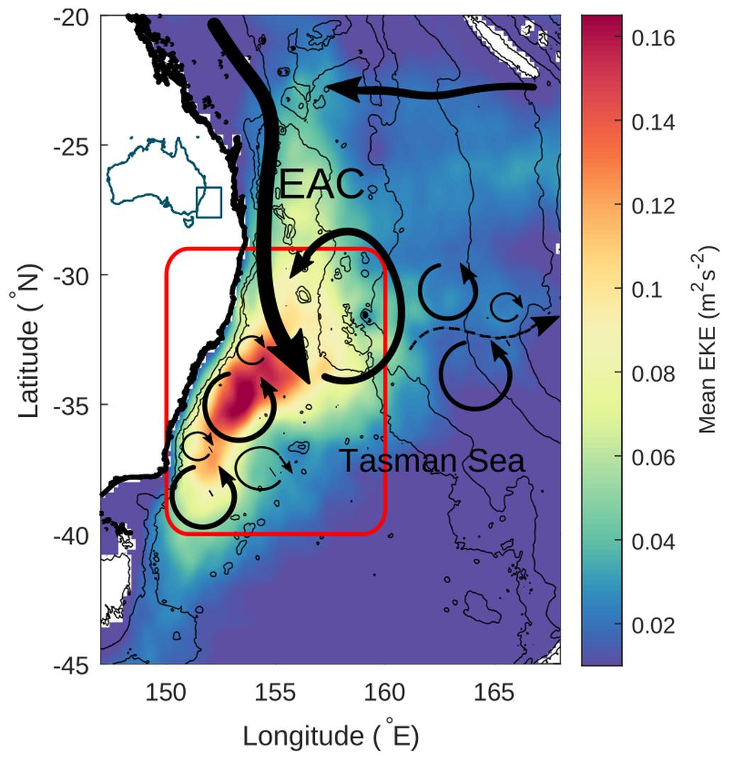
Figure 1. A schematic showing the boundaries of the region analyzed (red box). The mean eddy kinetic energy (EKE, 01/09/1981 to 30/12/2018) is shown with bathymetry contours (0, 200, and 2000 m). Inset shows the map of Australia and the location of the region in context. Arrows indicate the schematic of the mean circulation in the region. EAC stands for the East Australian Current.
It has been established that MHWs are not restricted to the surface but rather exhibit vertical warming that can have great effects in the subsurface. This was emphasized through response impacts like the coral bleaching during the Austral 2015/16 summer which occurred with no depth dependence, from 9 m down to 30 m (GBRMPA, 2016) and the large-scale decline of giant kelps (Oliver et al., 2017) given their sensitivity and direct response to ocean temperatures (Marzinelli et al., 2015). Jackson et al. (2018) also showed that abnormally warm water still lingered at depth in the Northeast Pacific Ocean and in river inlets on British Columbia’s central coast, 2 years after the end of the “Blob” MHW event at the surface. While this event was one of the most significant in the region, driven by anomalous air-sea heat flux and weak cold advection (Bond et al., 2015; Chen et al., 2015), Jackson et al. (2018) used Argo floats to show how subsurface warming (∼150 m depth) was delayed by about a year.
Few studies have focused on the depth structure of MHWs, due to the lack of sustained high-resolution temperature records below the surface. In the coastal Tasman Sea off Sydney, Schaeffer and Roughan (2017) studied the depth extent of warming (down to 100 m depths) during MHW events from long-term mooring observations. They found persistent extreme warming down the full extent of the water column at least 30% of the time, with maximum temperature anomalies occurring below the surface around the thermocline. Some deep MHW events did not have a surface signature hence SST variability was not representative of the vertical propagation of the MHW. Due to the coastal nature of the site, the major driver of deep MHW was downwelling favorable winds which depress the stratification enabling deeper mixing of warm surface waters. Conversely, upwelling events tend to suppress warm water anomalies with the intrusion of cold water. Further south, near Tasmania, Oliver et al. (2018b) used self organizing maps on modeling outputs to characterize the regional MHWs. They found that the average MHW depth was 90–185 m, with delays between the maximum anomalies at different depths. Types of MHWs were linked to a combination of anomalous EAC extension, offshore anticyclonic eddies, warm-air temperatures and wind anomalies from the north-westerly to easterly direction. Around the tropical Australia region, the longest MHW on record occurred in the Austral 15/16 summer and was documented by a range of regional observations (Oliver et al., 2017; Benthuysen et al., 2018) including in situ ocean gliders, Argo floats and moorings. The maximum anomalies occurred in March (end of the Austral summer) and at depth (∼60 m at a shelf mooring site), consistent with coral bleaching below the surface layer. A nearby Argo float measured positive temperature anomalies down to 300 m, showing the substantial depth extent of the MHW event. The authors attribute the record warming to surface heat flux anomalies (reduced cloud cover and weakened winds) during extreme El Niño and reduced Madden-Julian Oscillation conditions.
Despite these few studies, a full description of the depth extent of MHWs is still lacking. Furthermore, the factors affecting these subsurface extreme temperatures are still speculative, which together make it difficult to anticipate and prepare management responses to these extreme events.
The purpose of this paper is to provide the needed insight into MHW depth extent and the subsurface properties during a MHW. Here, we identify Argo floats during MHWs using SST time-series and utilize float observations extending down to 2000 m depth. We focus on the profiles of temperature and salinity anomalies and relate them to the ocean circulation in the western Tasman Sea, seasons, regions and drivers. Specifically, we address four aims: quantify “MHW depth” (see section “MHW Depth and Maximum Temperature Anomalies”), relate surface parameters and the subsurface extension (see section “Subsurface Properties in a MHW”), identify spatial or seasonal patterns (see section “Spatial and Seasonal Variability”), and drivers of the vertical structure of the MHW (see sections “Relationships Between MHW Depths and Profile Characteristics and Influence of Mesoscale Eddies”).
Materials and Methods
SST and MHW Identification
As in Benthuysen et al. (2018), Hobday et al. (2016), and Oliver et al. (2017) amongst others, SST observations were used to identify MHW events due to the lack of other daily in situ long time-series of temperature. SST was obtained from the daily National Oceanic and Atmospheric Administration Optimum Interpolation dataset gridded on a 0.25° grid (NOAA OI SST; Reynolds et al., 2007; Banzon et al., 2016), covering the period 01/09/1981-30/12/2018.
Applying the Hobday et al. (2016) definition of a MHW, as a discrete, prolonged and anomalous warm water event, MHWs were identified as events where temperatures exceeded the daily 90th percentile over five or more days. The climatology of the 90th percentile was calculated based on data for the period 01/09/1981-31/12/2018 for each day of the year using an 11-day window centered on that day, then smoothed with a 31-day moving average.
In situ Measurements and Climatology
Our defined study region is bounded by (150°E–160°E) and (40°S–29°S), covering the EAC extension area as indicated by the high kinetic energy (Figure 1). Mean eddy kinetic energy (EKE) is calculated using, , where u′ and v′ are the zonal and meridional anomalous surface geostrophic velocities (Richardson, 1983), calculated from gridded sea-level anomaly (GSLA). The data was sourced from the Integrated Marine Observing System (IMOS) for the period of 01/01/2004-30/12/2018 at 0.2° grid resolution which combines satellite altimeters and tide gauge observations (Deng et al., 2011).
In situ measurements were collected from available Argo float data within the region between 01/01/2004-31/12/2018. The processed data were obtained from the Australian Ocean Data Network portal (AODN) and include temperature, salinity and pressure profiles down to 2000 m depth. A total of 6550 Argo profiles were extracted.
Argo profiles were identified as MHW profiles if they were compiled during a MHW, otherwise, they were identified as NoMHW profiles. This was applied through the following process: all MHW event duration were identified from SST time-series for each profile location. If the temperature profile date (from Argo) fell within the MHW time-intervals, then it was determined a MHW water profile. Surface MHW events, their duration, intensity and category (as defined in Hobday et al. (2018)) were then extracted along with the Argo profile’s URL. This resulted in 894 water profiles in MHWs, providing a sufficient basis for analysis (Supplementary Figure S1).
Mean climatological profiles of temperature and salinity were obtained from the CSIRO Atlas of Regional Seas (CARS 2009) (Ridgway et al., 2002). Using linear interpolation, the gridded climatology profiles were calculated for each Argo profile by location and day of year. The CARS climatology encompasses mean ocean properties from all available quality-controlled historical subsurface measurements mapped to a 0.5° grid resolution. This climatology is used to compute the temperature anomaly , where T(z) is the temperature at depth z in the profile and is the climatological average. A similar procedure is employed for salinity (S′(z)) and density anomaly profiles.
A selection of the extracted MHW Argo water profiles was achieved by applying tests to remove any inconsistent profiles that either had missing fields or showed negative surface anomalies, which would contradict the positive anomaly indicated by the SST. Further, only profiles that contained observations extending down to 900 m depths or more were retained. Consequently, 39 out of the 894 MHW profiles were rendered unusable. Despite the different temporal periods for the SST (NOAA OI SST) and in situ climatology (CARS) datasets, no statistically significant difference was detected between the two surface averages in the datasets (mean square error of 0.15°C2).
Moreover, the surface temperature from Argo profiles and the extracted NOAA OI SST used to detect MHW events show a reasonable mean square error of 0.3°C2, most likely due to the different product resolutions. Additionally, residuals are found to be normally distributed and the correlation between the two parameters is r = 0.98 (Supplementary Figure S2). That is, no statistically significant difference was detected between the two measures and the assumptions of residual normality and constant variance are reasonable, justifying the link between SST and Argo float measurements.
Mixed Layer Depth
Climatological mixed layer depth (MLD) is also available from CARS and further calculated from Argo profiles, following the Condie and Dunn (2006) definition based on variations from surface temperature and salinity measurements at 10 m depths.
As such, MLD was determined as the minimum depth at which either (1) or (2) occur.
MHW Depth
All Argo MHW water column profiles were truncated at the first instance of a negative or zero temperature anomaly from the surface. The depth at which this occurs is defined as the positive threshold depth (denoted ZN hereafter), as follows,
The temperature anomaly profiles are long-tailed and positive anomalies are detected down to 2000 m in some profiles. However, the temperature is often almost homogenous (small vertical gradients) over 100 s of meters at depth (Figure 2). On this basis, we focus on vertical cumulative temperature anomaly (CTa) for each profile from the surface (z = 0) to its positive threshold depth (z = ZN) summed at 1 m spacing (Δz = 1) (Eq. 4). This measure also represents a scaled version of the anomalous heat content in the MHW (Willis et al., 2004; Dijkstra, 2008).
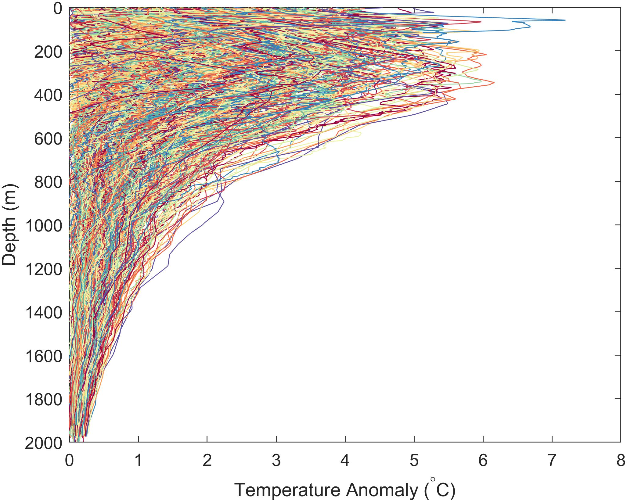
Figure 2. Temperature anomaly profiles in MHWs cut off at their respective Positive Threshold Depths.
In order to reduce the effect of the insignificant warming at depths per water profile, we define the MHW depth as the depth where a proportion (Ɛ, varied between 0.85–0.95) of the cumulative temperature anomaly is reached (Eq. 5).
Figure 3 illustrates this application on a single profile (top row) and on the mean profile (bottom row) with Ɛ values of 0.85, 0.9, and 0.95. In this particular example, positive anomalies are detected down to 2000 m and therefore the positive threshold depth is 2000 m. It is clear, however, that the profile changes at ∼1200 m with incrementally diminishing temperature anomalies toward the bottom of the profile (Figure 3B). In this case, ε = 0.9 (90% of the total warming in the water column up to its positive threshold) detects the onset of the small variation range in the profile that corresponds to a cumulative warming of 1749°Cm, which occurs at 1221 m depth and 0.39°C temperature anomaly in the profile. On the mean of all MHW profiles, ε = 0.9 produces an average MHW depth of 672 m occurring at an anomaly of ∼0.31°C and retains much of the significant warming while reducing the effect of the characteristic long tail in temperature anomaly profiles (Figure 3D). This is the desired outcome and is therefore chosen as the optimal threshold value for MHW depth.
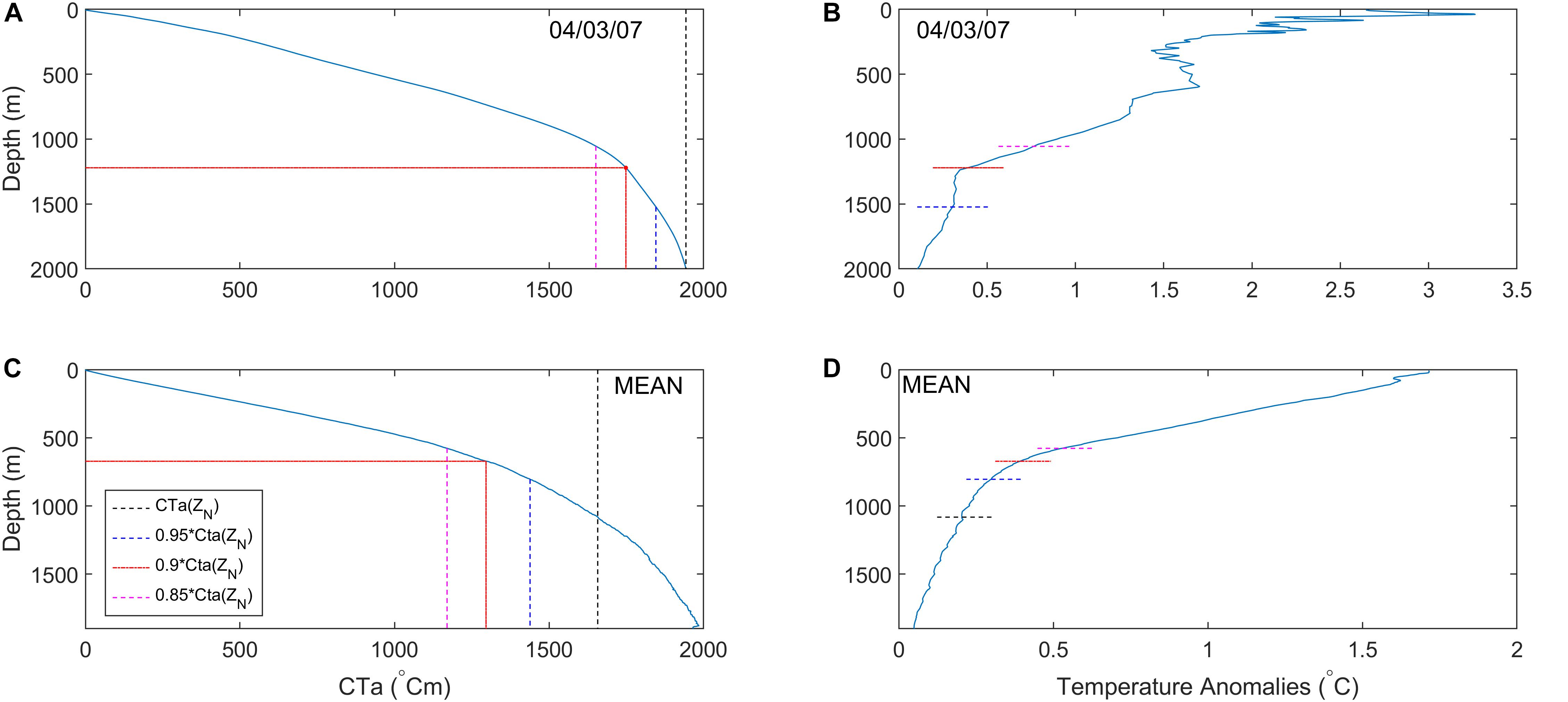
Figure 3. Illustration of different estimates of the MHW depth for a specific Argo profile (top row) with corresponding date of observation and the mean over all MHW profiles (bottom row). Panels (A,B) show the cumulative temperature anomaly (CTa) and the MHW depth obtained at ε = 0.95 (blue dotted line), 0.9 (red dotted-dashed line) and 0.85 (magenta dotted line). Panels (B,D) show the profiles of temperature anomaly and the corresponding MHW depth obtained using the CTa cut-offs at the same ε values.
A sensitivity analysis is conducted to test the robustness of different methods for measuring MHW depth cut-offs. The monthly variability of the MHW depth is used as a dependent variable and its sensitivity to the different methods is depicted in Figure 4. These methods include an arbitrary absolute temperature anomaly cut-off measure at 0.5°C, a cut-off value corresponding to the 10th percentile of the temperature anomaly profile (the depth below which 10% of the temperature observations are found), the positive threshold depth (ZN) and the above-mentioned thresholds with ε varied over the range of 0.85–0.95. The monthly means show that all MHW depth definitions exhibit similar monthly variability, but the signal is noisier with the methods using thresholds on absolute temperature anomalies (ZN and 0.5°C). In terms of magnitude, the MHW depths found vary over 100s of meters. The shallowest depths are found with the CTa threshold with ε = 0.85, and is very similar to the 0.5°C temperature anomaly cut-off. The deepest MHW depths are obtained when considering positive temperature anomalies (ZN) or the 10th percentile of the profile. For this study, we choose to consider the CTa with ε = 0.9, as it allows for the extraction of the depth where the abnormal heat significantly decreases (Figure 3) and it produces a meaningful (depth at which 90% of the abnormal cumulative heat is contained) and conservative MHW depth cut-off.
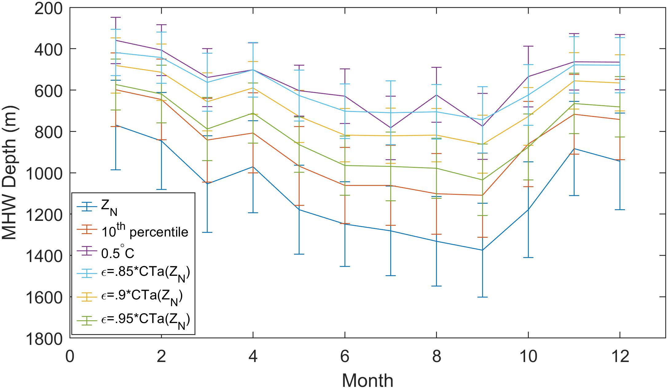
Figure 4. Sensitivity analysis: Mean MHW depth per month used as a dependent variable for testing the effect of different MHW depth cut-off methods. Positive Threshold Depth, 10th percentile (the value below which 10% of the observations are found), absolute value of temperature anomaly at 0.5°C and the CTa cut-off with ε = 0.95,0.9,0.85. Bars represent the standard errors.
Eddies
Using the framework expressed in Rykova and Oke (2015) for eddy detection and classification, GSLA was mapped around a 250 km radius of each water profile. Cyclonic (anticyclonic) eddies were detected within the radius if the minima (maxima) sea-level anomalies (SLA) were less (more) than −0.2 (0.2 m). Profiles are identified as being in neither eddies if no eddies were detected within their radius. Otherwise, profiles are in cyclonic (anticyclonic) eddies if the SLA at the Argo profile location is less than −0.02 (greater than 0.02) m and is monotonically decreasing (increasing) to the eddy extremum.
Results
MHW Depth and Maximum Temperature Anomalies
The calculated depths of the MHWs were highly variable, ranging from 10 m to 1522 m. Based on the distribution of the temperature profiles and the relationship with surface MHW properties (see section “Relationships Between MHW Depths and Profile Characteristics”), MHWs are divided into three categories (Figure 5), namely category 1 (shallow, 0–150 m deep), consistent with the heat capacity of the ocean mixed layer (Schwartz, 2007), category 2 (intermediate, 150–800 m deep) and category 3 (deep, depth >800 m). Note that the peak for MHW depth that occurs in the higher range depths is likely due to the influence of the profiles which are warmer than climatology all the way down to the deepest (2000 m) Argo measurement. This, however, does not have an implication on our results given that these characteristics are captured within the category thresholds.
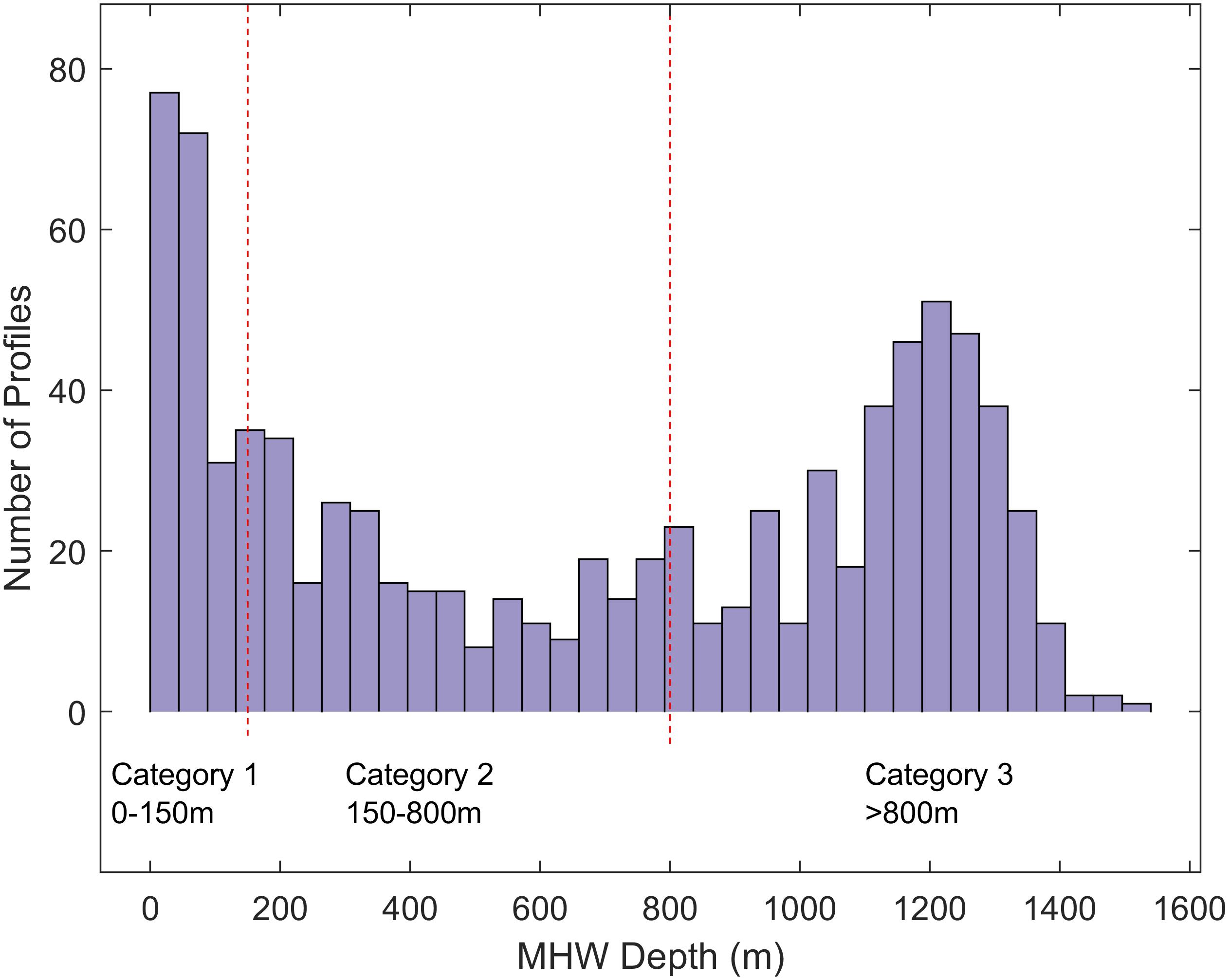
Figure 5. Marine heatwave depth for Argo float profiles. Three categories were identified: 0–150 m (shallow), 150–800 m (intermediate) and >800 m (deep). Depths bins have 50 m spacing.
Only 23% of the total MHWs are restricted to the surface layers (category 1, average of 63 m deep, Table 1), while almost half (∼45%) show a significant temperature anomaly deeper than 800 m (category 3, average of 1146 m deep, Table 1). Although, the highest frequency of MHW depth is less than 50 m deep (∼80 profiles, Figure 5). The three categories also have different MHW durations with the deepest MHWs lasting longest on average (27 days compared to 20 days) (Supplementary Figure S3, Table 1).
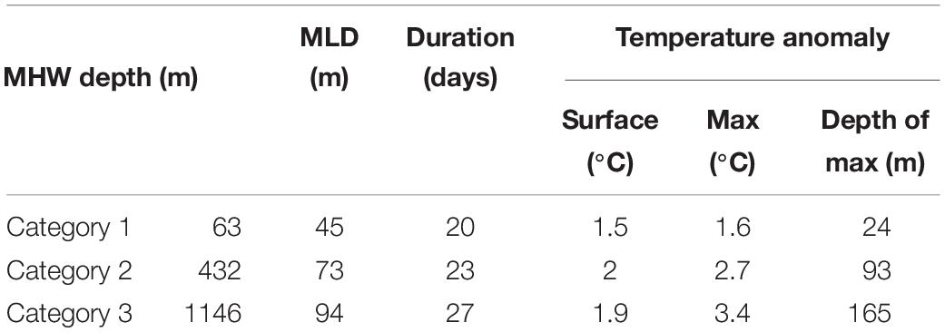
Table 1. Mean characteristics of MHWs in categories 1 (0–150 m), 2 (150–800 m), and 3 (800–2000 m) from Argo data: depth extent, mixed layer depth, duration, sea-surface temperature anomaly (Surface, from SST and Argo floats), maximum temperature anomaly (Max) and the depth where it occurs (Depth of Max).
The temperature anomaly profiles within each MHW category are distinctively different and suggest that varying mechanisms are driving these extreme events (Figure 6). Shallow MHWs (category 1) tend to show a decreasing warming in the top 100 m. The maximum temperature anomaly is close to the surface (24 m) around 1.6°C, similar to the SST anomaly of 1.5°C (average across all profiles). It is notable that many profiles are anomalously cooler below the MHW depth in this category (Figure 6A and Supplementary Figure S4), however, for the purpose of this study we focus on the warming depths in a MHW. In contrast, the mean profile of deep MHWs (category 3) has a greater subsurface temperature anomaly of 3.4°C, twice the maximum anomaly in category 1 and peaks at depth (mean of 165 m). Interestingly, the magnitudes of the surface temperature anomalies across all categories are similar (1.5–2°C), suggesting that distinct intense MHW patterns cannot be differentiated when only looking at the surface (Table 1). Category 2 shows a mix of the previous characteristics, with a slight increasing temperature anomaly in the top 93 m in the mean, where the maximum anomaly occurs before decaying.
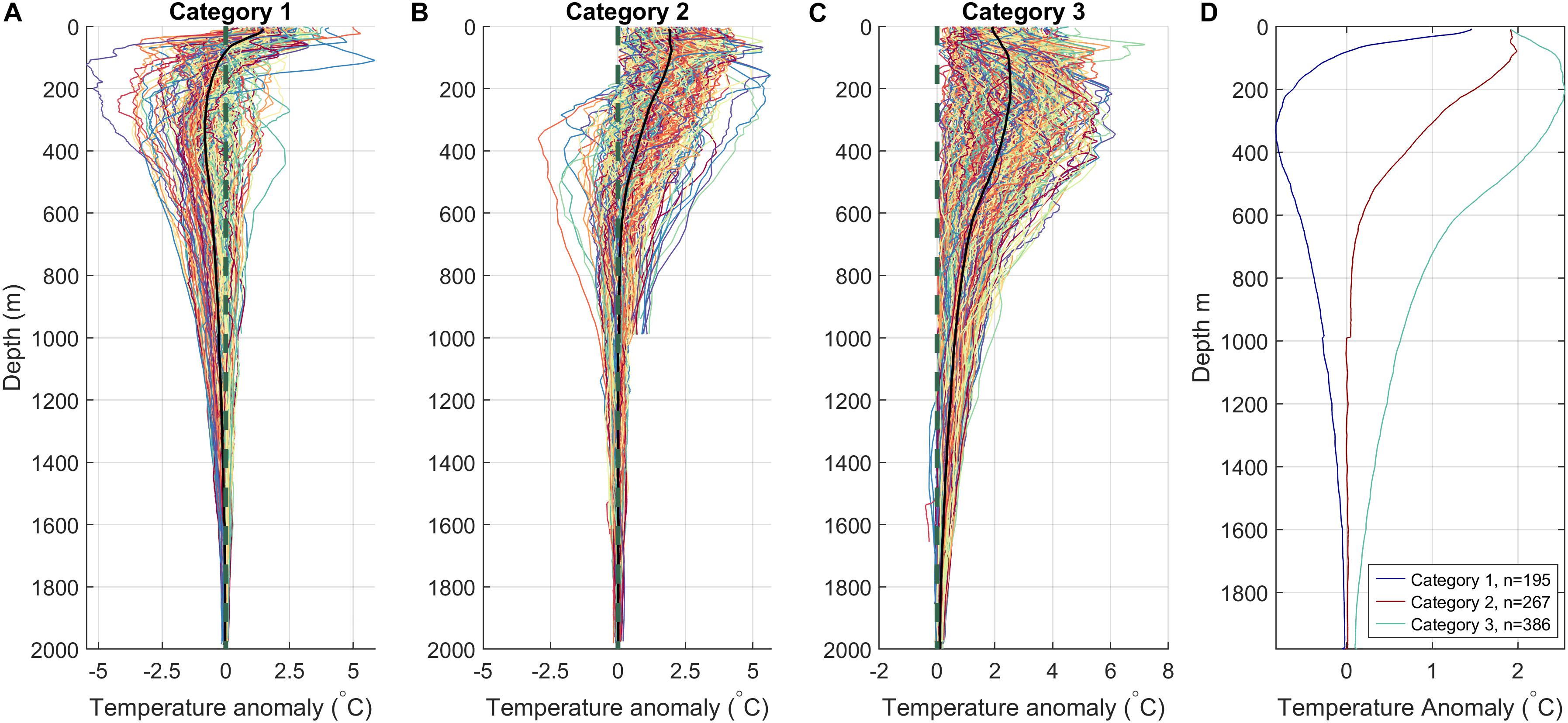
Figure 6. Individual (colored lines) and mean (thick black lines) depth profiles of temperature anomalies during MHWs of category 1 (A), 2 (B), and 3 (C). Gray dashed line shows the positive threshold anomaly. Panel (D) shows the mean temperature anomaly profile per MHW category with the number of Argo profiles per category indicated in the legend.
Subsurface Properties in a MHW
Using CARS climatology, characteristics of density and salinity anomalies during a MHW at depth are also investigated. In the top 100 m, MHWs are on average fresher than climatology (Figure 7A) most likely due to the long-term trends identified by Rykova and Oke (2015). They showed using Argo in situ measurements and models, that since 2005 the Tasman Sea surface region has freshened in response to increased precipitation off Eastern Australia. Below 100 m, MHWs have various signatures which appear related to the overall depth of the extreme warming. Category 1 freshens below the MHW depth reaching a maximum at ∼250 m and decaying to ∼700 m. This freshness is consistent with the aforementioned cooling found below the MHW depth in this category, leading to an unchanged density (Figure 7B). Whereas categories 2 and 3 become saltier down to ∼650 m and ∼900 m, respectively, with anomalies peaking at 0.26 PSU on average for the latter. In terms of density (Figure 7B), the profiles are similar to the temperature profiles due to the predominant influence of temperature on density variability in the region, characterized by lighter water-mass in the range of warm temperature anomalies for the intermediate and deep MHWs.
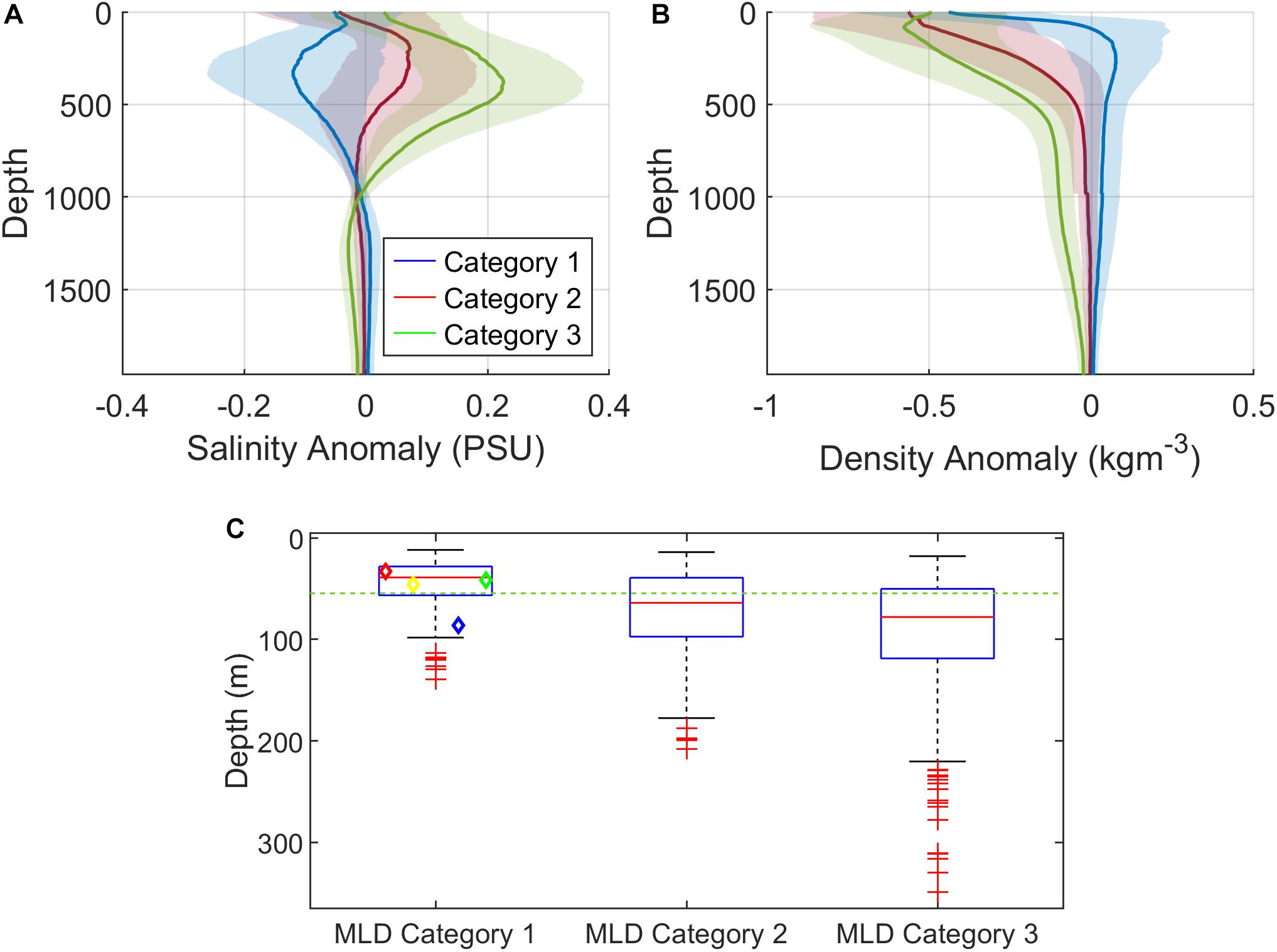
Figure 7. Standard deviation (shading) and mean (thick lines) show the spread of salinity (A) and density (B) anomalies during MHWs per category. Panel (C) shows the median, standard deviation and 25th–75th percentiles of the MLD during MHWs of category 1, 2, and 3. Category 1 seasonal MLD is indicated by colored diamonds (summer DJF, autumn MAM, winter JJA and spring SON shown with red, yellow, blue and green diamonds, respectively). The mean climatological MLD in the region (57 m) is shown for reference with a dashed green line. Outliers are indicated with red crosses.
Compared to climatology, the MLDs (Figure 7C) for category 1 MHWs are shallower with a median at 39 m compared to climatological MLD at 57 m, meaning the water column is more stratified. Category 1 seasonal MLDs (as shown by colored diamonds) appear to behave as expected in this region with the seasonal variation centering around the median and category 1 matching the most stratified months. Category 3 median MLD is much deeper at 78 m, showing more mixing and less stratification in the water columns while category 2 is almost equivalent to that of climatology. That is, shallow MLDs correspond with shallow MHWs and progressively deepen with MHW depth.
Spatial and Seasonal Variability
Spatially, the incidence of category 2 and 3 MHWs varies with latitude. Southward of 32°S, all three categories occur whilst the deepest MHWs dominate the region between 32°S and 38°S (Figure 8A), corresponding to the area of maximum EKE (Figure 1). Northward of 32°S, deep MHWs (category 3) become less frequent with category 2 dominating the region, which coincides with the mean location of the eastward extension of the EAC (Tasman Front) which occurs at around 32°S (Oke et al., 2019 and Figure 1). Shallow MHWs are the most frequent below 38°S, south of the maximum EKE.
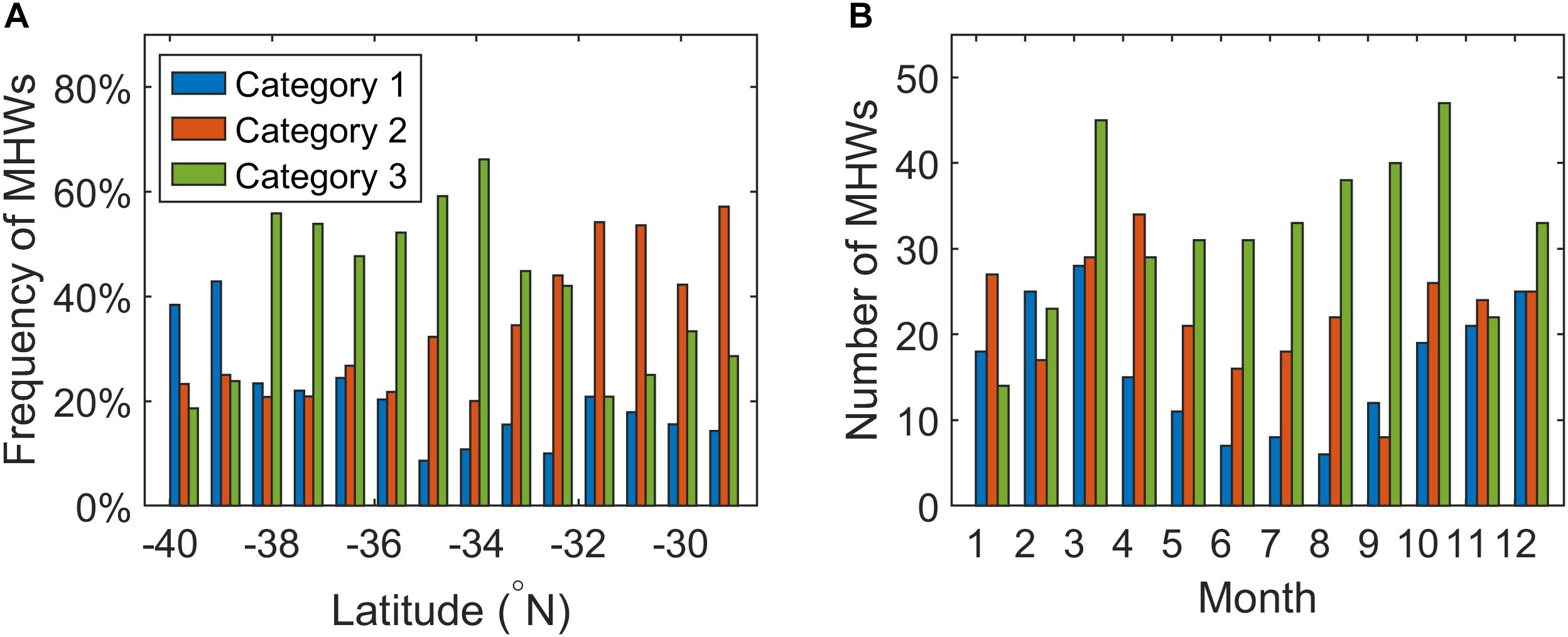
Figure 8. Latitudinal (A) and monthly (B) distribution of Argo float profiles during MHWs for shallow (category 1), intermediate (category 2) and deep (category 3) events.
In terms of temporal variability, MHWs occur all year round but their depth and intensity in the region vary seasonally (Figure 8B). Note that CARS climatology includes seasonality, that is, the anomalies investigated here are with respect to the characteristic seasonality of water profiles. Shallow MHWs tend to occur preferentially in the austral summer and autumn (October–April) when the water column is the most stratified. MHWs are deeper in spring and winter, although categories 2 and 3 still occur year round. Looking at the mean profiles of all MHWs per season (Figure 9), winter is characterized by warmer and deeper anomalies that are consistent with mostly deep MHW events. The mean anomalies reach a maximum intensity of 1.9°C at 200 m and 0.14 PSU at 384 m in winter, with July being the most intense reaching a temperature anomaly of 2.7°C. The depth structure in MHWs in spring and summer behave similarly whereby temperature anomalies decay from near the surface, with summer having warmer surface temperatures and cooling more quickly with depth than spring. Autumn shows a subsurface temperature maximum similar to winter with slightly less intensity of ∼1.8°C and at a shallower depth of ∼100 m. MHWs in summer and autumn are fresher at the surface, whilst there is no significant surface salinity signal in spring. The most saline surface occurs in winter. The composite plot in Figure 9C shows the annual cycle of temperature anomalies versus depth, illustrating the deepening intensity in temperature anomalies in particular around the July and September months and the link between MLD and the depth of maximum temperature anomalies.
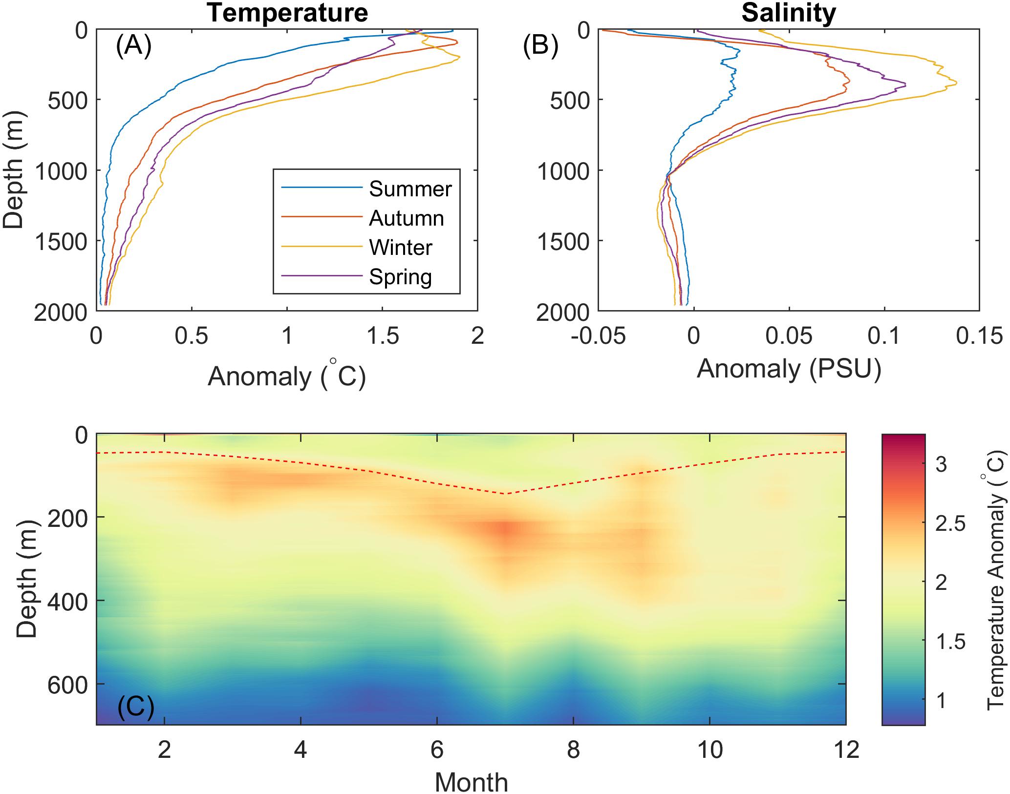
Figure 9. Mean seasonal depth profiles of temperature (A) and salinity (B) anomalies during MHWs. (C) Monthly composites of temperature anomaly during MHWs. The monthly mean MLD (red dashed line) is overlaid.
Relationships Between MHW Depths and Profile Characteristics
Statistically, the MHW depth is only related to the surface temperature in the case of shallow MHWs. For category 1 (MHWs shallower than 150 m) we find a positive, statistically significant relationship between the surface temperature anomaly and the MHW depth penetration with a correlation of 0.3 (p-value < 0.00001) showing that the more intense the surface warming is, the deeper it penetrates (Supplementary Figure S5). However, the depth of categories 2 and 3 is not related to the surface temperature anomaly, thus this relationship only holds for shallow MHWs. That is, the intensity of surface warming is limited to indicating shallow MHWs depths to some extent and is not a prognostic tool for MHWs that extend deeper than ∼150 m in the water columns.
Significant relationships are, however, found between MHW depth and the characteristics of the water’s vertical profile for all MHW categories (Figure 10). The deeper the MHW is, the deeper and greater the maximum temperature anomaly is (correlation of 0.5 and 0.52 with p-value < 0.0001, respectively). It is interesting to note that salinity exhibits distinct behavior across the MHW categories. Consistent with the previously described characteristic of cooling and freshening below category 1 MHWs (see section “MHW Depth and Maximum Temperature Anomalies”), shallow MHWs are distinctively freshest at depth but show no relationship between freshness (negative salinity anomalies) and MHW depth. On the other hand, deep MHWs tend to be anomalously saltier with a strong relationship to MHW depth over all categories (r = 0.67, p-value < 0.0001). MLD has a slightly weaker relationship with MHW depth but still shows a significant correlation at r = 0.4 (p-value < 0.0001). A principal component analysis (PCA), following the Emery and Thomson (2001) framework, also confirms the relationships found here, with the strongest being the maximum salinity anomaly and the weakest being the SST anomaly (Supplementary Figure S6). Therefore, subsurface characteristics are a more reliable indicator of the vertical warming extent, with salinity being a strong discriminator.
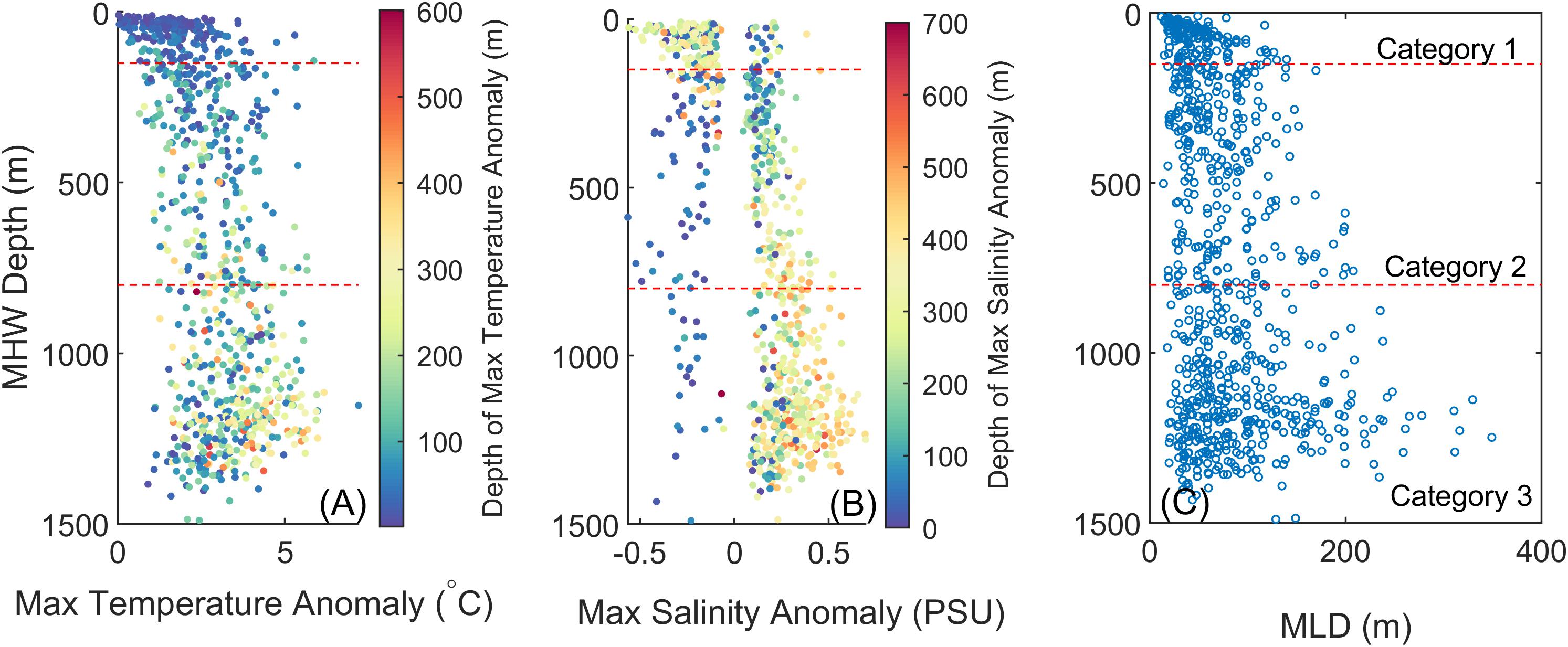
Figure 10. Scatter plots of MHW depth against (A) maximum temperature anomaly, (B) extremum salinity anomaly and (C) MLD. Colors in panel (A,C) show the depth where the extrema occur.
Influence of Mesoscale Eddies
Consistent with the western Tasman Sea being an eddy-dominated region (Figure 1), 84% of the MHWs studied were found in eddies with 88% of those in warm core eddies (WCE). Figure 11 shows an example of three individual Argo profiles sampling MHWs within a WCE (anticyclonic), a cold core eddy (CCE) (cyclonic) and no eddy. The profile sampling in a WCE (column 1) has the deepest MHW depth at 771 m while the CCE (column 3) is shallowest at 125 m.
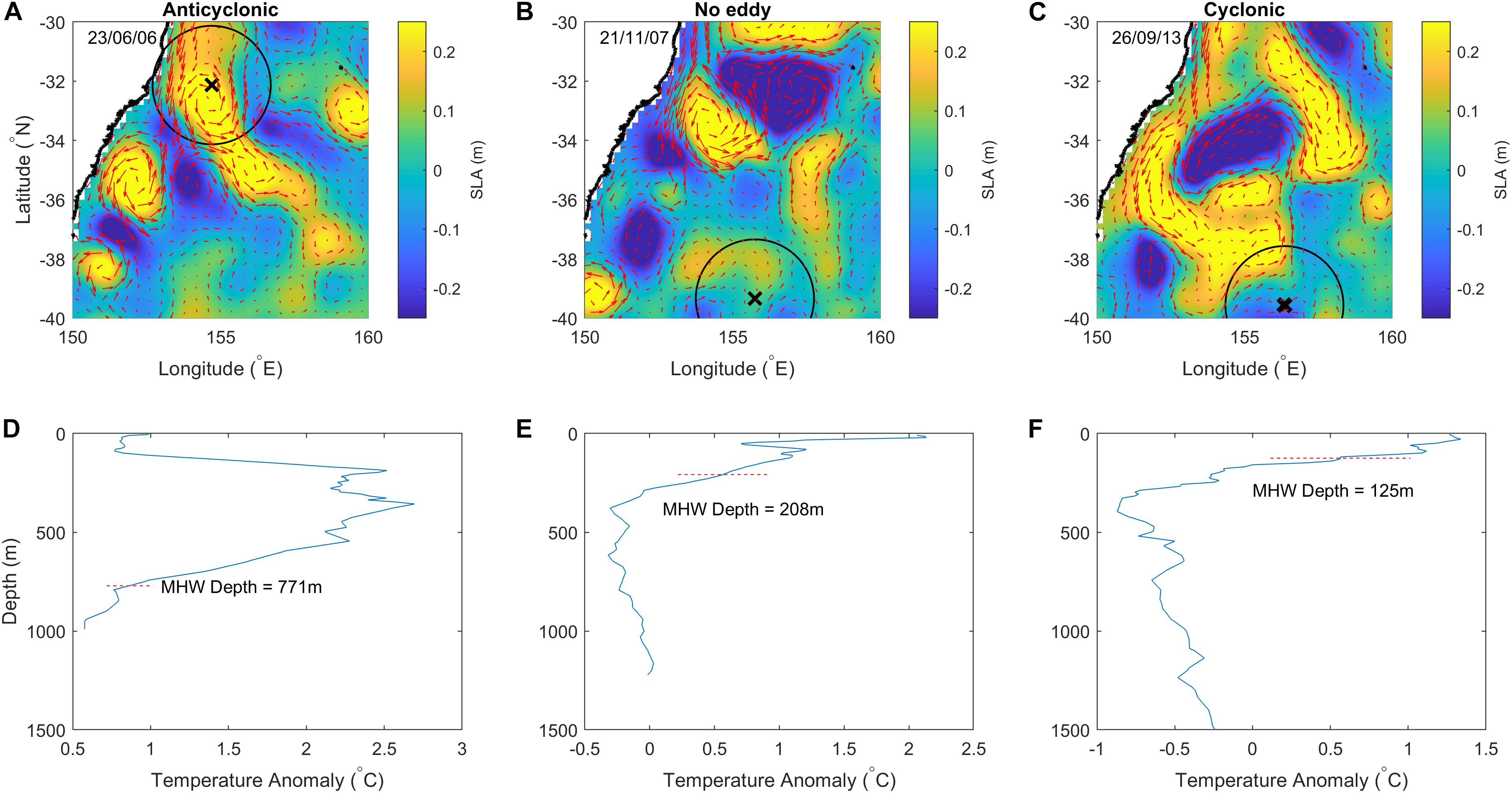
Figure 11. Examples of Argo floats in an anticyclonic (A,D), no eddy (B,E), and cyclonic (C,F) eddy for specific dates. Top panels show the corresponding sea level anomaly (SLA) and geostrophic currents with the location of the Argo float (black cross). Bottom panels show the Argo float temperature anomaly profile and the corresponding calculated MHW depth. The marked circle around the Argo float outlines the 250 km radius used to search for nearby eddies.
In fact, the MHW depth is strongly correlated to the corresponding SLA extracted from altimetry (Figure 12A, r = 0.62 and p < 0.0001) consistent with the findings of Rykova and Oke (2015) on the relationship between SLA intensity, the temperature anomaly intensity and depth of the eddy core. Figure 12A shows the breakdown of eddy conditions per category and while most category 2 and 3 MHWs (deeper than 150 m) were found within anticyclonic eddies, it is interesting to see that category 1 MHWs occur across a mix of ocean conditions, suggesting different drivers for the shallow MHWs. In particular, vertical warming during MHWs also occurs in cyclonic eddies, meaning their cold characteristic does not necessarily suppress the extreme warming during the MHW, although they do occur at a lesser frequency of 5% as opposed to 21% in WCEs. Note, the hollow circles in Figure 12A are of those profiles that were detected in eddy conditions and failed the monotonically increasing/decreasing test to the eddy extremum. Failing this test, however, does not prove that the profiles are in neither eddy conditions and therefore their statistics are not included in the eddy condition categories.
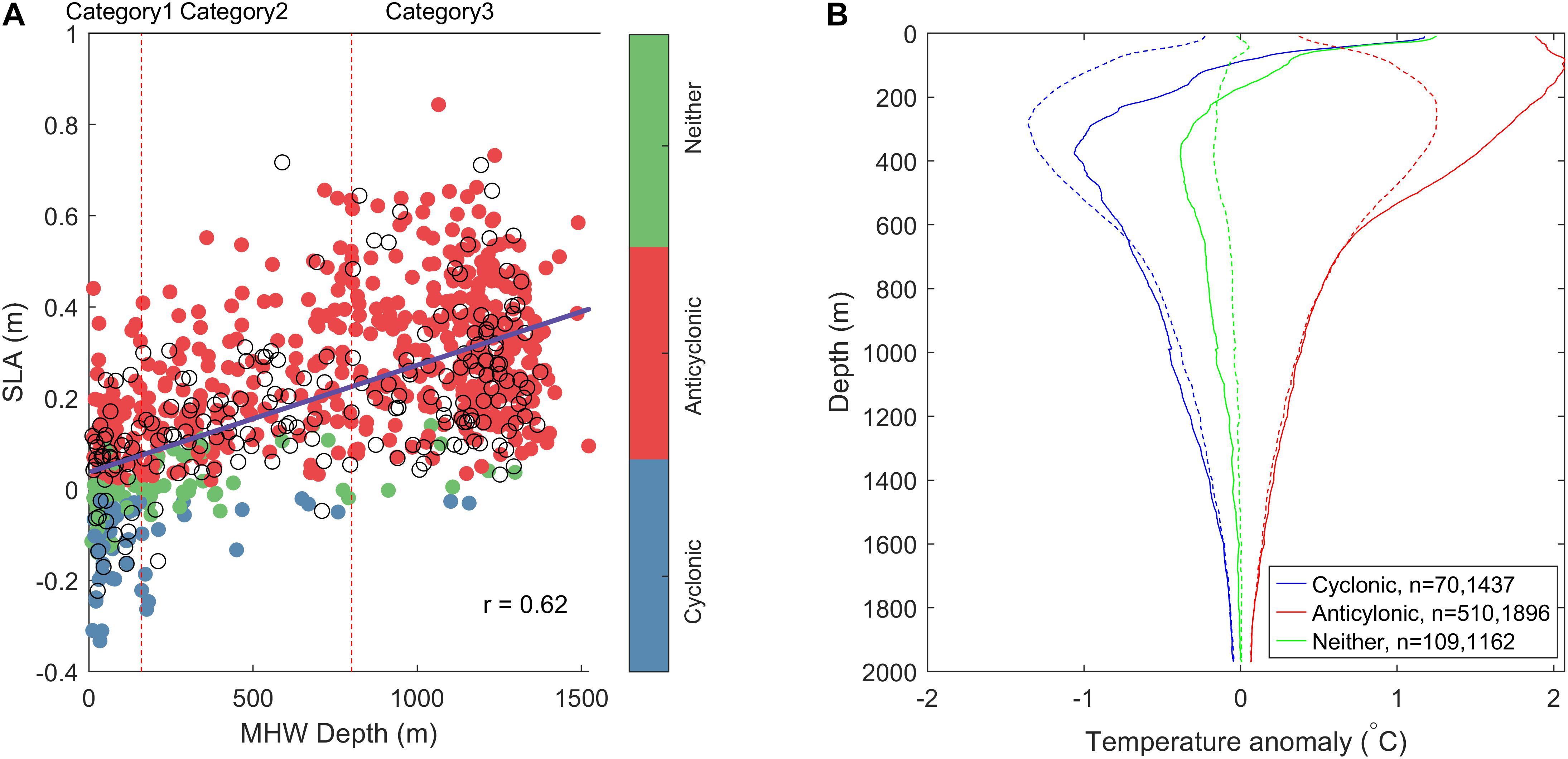
Figure 12. (A) Scatter plot of sea level anomaly (SLA) and MHW depth. Colors indicate whether the water profile is in a cyclonic eddy (blue) an anticyclonic eddy (red) or not in an eddy (green). Hollow circles represent non-significant SLA. The regression line between SLA and MHW depth and correlation coefficient are indicated. Category thresholds are depicted by the top x-axis. (B) Mean temperature anomaly profiles per eddy type: cyclonic (blue line), anticyclonic (red line) and not in an eddy (green line) averaged for MHW (solid) and NoMHW (dashed) Argo floats. Number of profiles per category are indicated in the legend for MHWs and NoMHWs, respectively.
It has been shown that WCEs have a deeper MLD especially in winter based on their seasonality (Tranter et al., 1980; Brenner et al., 1991; Kouketsu et al., 2011). Given the predominance of MHWs occurring in WCE, this effect is evident in the MHW MLD (Figure 7C). In the region, WCEs typically have a warm core of 2–4°C at depths of around 300–350 m while the mean CCEs have a cold core centered around 250–350 m with −1.5 to −4°C temperature anomalies (Rykova and Oke, 2015). These eddy characteristics are consistent with the mean profile in eddies found here. Figure 12B illustrates the differences between mean temperature profiles in MHWs (solid lines) and NoMHWs (dashed lines) in the various eddy conditions. The influence of the MHW within eddies is clear with a significant warming in the top ∼600 m on average overlaid to the typical structures. This additional warming leads to positive anomalies in the surface layers for CCEs and duplicates the positive temperature anomaly in WCEs at higher temperature intensities (∼1.5°C warmer down to ∼300 m). Profiles outside of eddies tend to show a warming in the top ∼200 m during MHWs and a slight cooling at greater depths.
Seasonality of eddy conditions and profiles within (Figure 13A) and out of MHWs show that most of the NoMHW profiles are found within WCE and CCE (Figure 13B), confirming that eddies are not the sole contributors to warm anomalies at depths but rather function as a catalyst to drive warm anomalies deeper during an existing MHW event. MHWs in CCEs exhibit a seasonal cycle predominantly occurring in summer and spring while MHWs in WCE are more frequent in the first half of the year.
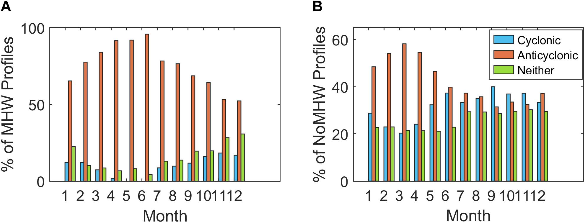
Figure 13. Monthly distributions of Argo profiles in cyclonic (blue), anticyclonic (yellow) eddies or neither (red) during MHWs (A) and NoMHWs (B).
Discussion
This study reveals that, contrary to common understanding, MHWs in the Tasman Sea can extend to 1500 m. MHWs frequently extend much deeper than the MLD, regardless of the definition used for the MHW depth. When applying the cumulative temperature anomaly threshold, we have showed that MHWs have a mean depth of 672 m with anomalous warming reaching down to 1522 m. In comparison, focusing on positive anomalies leads to warming detected down to >2000 m. The definition using a percentage threshold for the CTa appears to be most fitting because it is more conservative and meaningful than an absolute value (or percentile) of positive temperature anomaly. Moreover, the application of the CTa threshold reduces the potential risk of bias that can be associated with a positive threshold anomaly given its sensitivity to measuring the very gradual warming effect expected in the deep ocean (Roemmich et al., 2015).
Shallow MHWs restricted to the surface layers (<150 m) only represent 23% of the Argo profiles. They occur predominantly in summer/autumn in various mesoscale structures (cyclonic, anticyclonic or no eddies) and their depth is correlated with the SST anomaly. These events are characterized by stratified and fresh surface waters, suggesting that there is a predominant air-sea flux forcing whereby anomalous solar radiation and decreased wind stress act on latent heat-flux to reduce evaporation (Chen et al., 2014, 2015; Bond et al., 2015; Benthuysen et al., 2018). Interestingly, when the domain is restricted to the high eddy field region only [(150°E,157°E) and (37°S,29°S)], the correlation coefficient between surface temperature anomalies and shallow MHW depth increases to 0.6 (as opposed to 0.3), that is, shallow MHWs are more sensitive to the region’s characteristics.
In contrast, deep MHWs (>800 m) almost exclusively occur in anticyclonic warm core eddies, all year round but predominantly in winter south of the Tasman Front. They are characterized by a deeper MLD, a freshening in the top 100 m under which the water-mass is more saline (between 100 and 900 m), which is consistent with WCEs in the Tasman Sea (Rykova and Oke, 2015). Depth for deep MHWs is not related to surface conditions, however, it is directly related to the water-mass’s anomalies, where the deeper the MHW extends, the deeper and more intense the temperature and salinity anomalies become. The lack of correlation between MHW surface temperature and depth characteristics is consistent with Brenner et al. (1991) who found a similar result for eddies in summer. By comparison, a strong relationship exists between SLA and MHW depth due to the steric height of the warm water column. It should, however, be noted that MHWs in eddies are still rare events since most of the Argo float profiles in WCEs sampled regular temperatures.
Due to a lack of long-term in situ observations, this study is limited to the analysis of the vertical extensions of MHWs that are identifiable by anomalous SST. As Schaeffer and Roughan (2017) showed on the Sydney continental shelf, not all MHWs are detectable at the surface. The signatures of such MHWs are of great interest and further studies in this topic using subsurface detection methods are essential to grasp a more complete picture of MHW dissemination. Since in situ daily observations over decades [as recommended by Hobday et al. (2016)] do not exist in the open ocean, ocean modeling is necessary to investigate the full three-dimensional dynamics of the heat flux budgets.
In terms of inter-annual variability, our study’s 14 year span (limited by the Argo era) is too short to draw conclusions; however, a deepening trend can be seen in both the yearly averaged maximum temperature anomalies and MHW depth (Figure 14). In this region, the El Niño Southern Oscillation (ENSO) index is only weakly related to local SST (Holbrook and Maharaj, 2008; Shears and Bowen, 2017), however, some of the more intense MHWs further south occurred during simultaneously strong El Niño events like the Austral Summer 2015/16 MHW (Oliver et al., 2017). Despite the coexistence of these events, the authors found that the El Niño had only a modest role on the MHW event in the Tasman Sea region due to its limited influence on EAC transport (Oliver et al., 2017). On the other hand, Heidemann and Ribbe (2019) recently found significant correlations (∼0.35) between SST anomalies and ENSO (with a 7-month lag) in Southern Queensland, leading to more MHW days during El Niño years. While the link between the EAC, its eddies, the Tasman Sea SST and ENSO is still unclear, Figure 14 suggests a deepening of MHWs during strong El Niño years [2006, 2009, 2014–2016, defined as a sustained Southern Oscillation Index (SOI) exceeding +7, BoM (2017)]. This potential connection needs to be considered through additional investigation where longer time-series are available for the dynamical link to be understood.
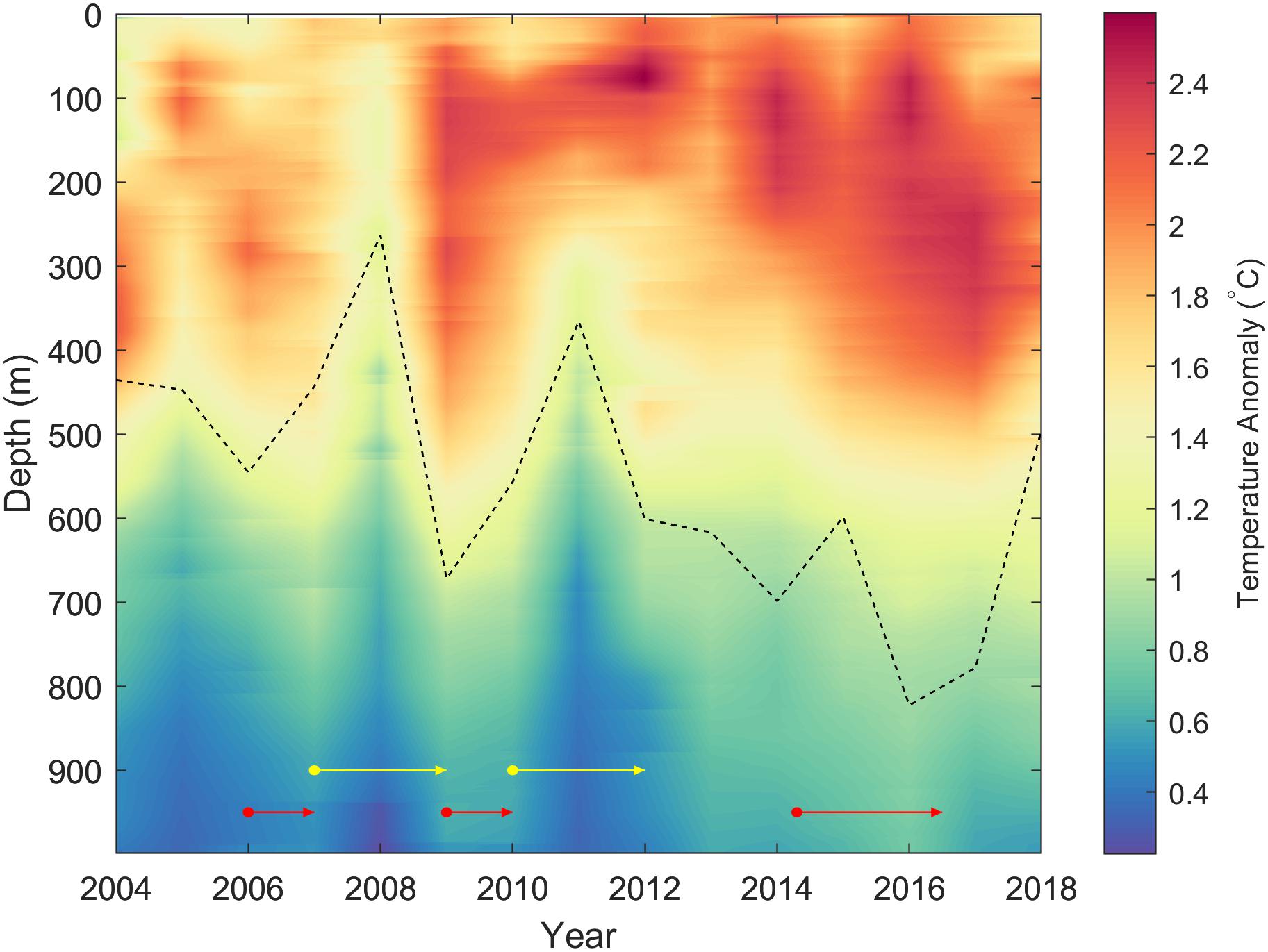
Figure 14. Yearly composite of temperature anomaly in MHWs. The annual mean of MHW depth (thick black line) is overlaid. Arrows indicating major El Niño (red) and La Niña (yellow) events are shown. ENSO events are identified using SOI monthly (BOM) where maxima exceed ±7.
It is reasonable to posit that the discernible links between MHW depth and their drivers presented here are likely to apply mostly in the case of short term events (the mean duration here is around 3 weeks) and when MHWs are located offshore as opposed to year-long or coastal. In fact, in coastal areas like the ones considered by Schaeffer and Roughan (2017) and Oliver et al. (2018b), short term (days-weeks) events were found to be driven by wind stress anomaly, in particular downwelling winds that influenced the vertical mixing and MLD, resulting in deeper MHWs. In the case of long-term events the connection between MHW depth and single drivers is most likely less detectable. Studies on year-long record events (as opposed to a mean duration of 20–27 days as found in this study) find a broad range of interactions since a broader range of processes are likely to interact while overlapping with the inter-annual variability expected (Feng et al., 2013; Benthuysen et al., 2014, 2018; Oliver et al., 2017). In this case, the depth of the extreme warming may vary locally during the event and the relationship we identified may not be applicable.
Given that intermittent warming can have a more damaging effect on the marine habitat than gradual ocean warming (Oliver et al., 2018a), the detection of warm anomalous waters at extreme depths found here suggests that the mesopelagic habitat could also be impacted. Temperature is one of the main environmental drivers influencing shark abundance (Lee et al., 2018) and we can expect deep extreme temperatures to affect the behavior of some of the local megafauna. Climate change has already been established to cause irreversible redistribution in the coastal benthic species (Ling, 2008; Johnson et al., 2011) and on this basis, it is conceivable that the intermittent warming brought about by MHWs causes comparatively more damage within the anomalous warming depth range.
In summary, this paper finds MHWs extending to extreme depths with no detectable surface signal and substantial eddy influence on warming extensions. The results highlight the fact that the surface characteristics of MHWs based on SST only inform anomalies in the water column if the MHW is shallow and most likely surface-forced, independent from the ocean circulation. This has been the primary indicator for most studies to date, however, in light of our results, SST is an insufficient proxy for anomalous warming at depth. Further, given the eddy abundance in the Tasman Sea region, mesoscale ocean dynamics need to be considered to allow meaningful supposition as to the water-mass profile at great depths. As such, we recommend a simultaneous analysis of SST and SLA to investigate and potentially predict future MHWs particularly in eddy-dominated regions such as the Western Boundary Current extensions, e.g., off the Gulf stream (Leterme and Pingree, 2008) and the Kuroshio–Oyashio Confluence region (Sugimoto et al., 2017). Ultimately, this will improve our understanding of subsurface biological impacts and the management actions necessary to work toward preventing irreversible impacts on the ocean ecosystem.
Data Availability Statement
Publicly available datasets were analyzed in this study. This data can be found here: https://portal.aodn.org.au/, https://www.esrl.noaa.gov/psd/, www.cmar.csiro.au/cars and www.bom.gov.au. The Argo data were downloaded from the Australian Ocean Data Network portal (https://portal.aodn.org.au/) and Argo GDAC Data Browser (https://www.usgodae.org/cgi-bin/argo_select.pl), and these data are collected and made freely available by the International Argo Program and the national programs that contribute to it (http://www.Argo.ucsd.edu, http://Argo.jcommops.org). The Argo Program is part of the Global Ocean Observing System. Data for altimetry was obtained through the Australian Ocean Data Network portal (https://portal.aodn.org.au/) from the Integrated Marine Observing System (IMOS) – IMOS is a national collaborative research infrastructure, supported by the Australian Government. CARS2009 Climatology data were obtained from CSIRO Marine Laboratories from www.cmar.csiro.au/cars. NOAA_OI_SST_V2 data provided by the NOAA/OAR/ESRL PSD, Boulder, Colorado, United States, from their Website at https://www.esrl.noaa.gov/psd/. The Southern Oscillation Index (SOI) for ENSO events shown in Figure 14 were obtained from the © Bureau of Meterology, www.bom.gov.au.
Author Contributions
YE performed the analysis and wrote most of the manuscript as part as her Master research project. AS supervised, proposed and guided the project, and took part in the writing.
Conflict of Interest
The authors declare that the research was conducted in the absence of any commercial or financial relationships that could be construed as a potential conflict of interest.
Supplementary Material
The Supplementary Material for this article can be found online at: https://www.frontiersin.org/articles/10.3389/fmars.2019.00745/full#supplementary-material
References
Banzon, V., Smith, T. M., Chin, T. M., Liu, C., and Hankins, W. (2016). A long-term record of blended satellite and in situ sea-surface temperature for climate monitoring, modeling and environmental studies. Earth Syst. Sci. Data 8, 165–176. doi: 10.5194/essd-8-165-2016
Benthuysen, J., Feng, M., and Zhong, L. (2014). Spatial patterns of warming off Western Australia during the 2011 Ningaloo Niño: quantifying impacts of remote and local forcing. Cont. Shelf Res. 91, 232–246. doi: 10.1016/j.csr.2014.09.014
Benthuysen, J. A., Oliver, E. C. J., Feng, M., and Marshall, A. G. (2018). Extreme marine warming across tropical Australia during austral summer 2015–2016. J. Geophys. Res. Oceans 123, 1301–1326. doi: 10.1002/2017JC013326
BoM (2017). ENSO Outlook: An Alert System for the El Niño–Southern Oscillation. Available at: www.bom.gov.au/climate/enso/outlook/#tabs=Criteria (accessed December 17, 2018).
Bond, N. A., Cronin, M. F., Freeland, H., and Mantua, N. (2015). Causes and impacts of the 2014 warm anomaly in the NE Pacific. Geophys. Res. Lett. 42, 414–420. doi: 10.1002/2015GL063306
Brenner, S., Rozentraub, Z., Bishop, J., and Krom, M. (1991). The mixed-layer/thermocline cycle of a persistent warm core eddy in the eastern Mediterranean. Dyn. Atmos. Oceans 15, 457–476. doi: 10.1016/0377-0265(91)90028-E
Cai, W. J., Shi, G., Cowan, T., Bi, D., and Ribbe, J. (2005). The response of the Southern annular mode, the East Australian current, and the southern mid-latitude ocean circulation to global warming. Geophys. Res. Lett. 32:L23706. doi: 10.1029/2005GL024701
Cerrano, C., Bavestrello, G., Bianchi, C., Cattaneo-vietti, R., Bava, S., Morganti, C., et al. (2000). A catastrophic mass-mortality episode of gorgonians and other organisms in the Ligurian Sea (North-western Mediterranean), summer 1999. Ecol. Lett. 3, 284–293. doi: 10.1046/j.1461-0248.2000.00152.x
Chen, K., Gawarkiewicz, G., Kwon, Y. O., and Zhang, W. G. (2015). The role of atmospheric forcing versus ocean advection during the extreme warming of the Northeast U.S. continental shelf in 2012. J. Geophys. Res. Oceans 120, 4324–4339. doi: 10.1002/2014JC010547
Chen, K., Gawarkiewicz, G. G., Lentz, S. J., and Bane, J. M. (2014). Diagnosing the warming of the Northeastern U.S. Coastal Ocean in 2012: a linkage between the atmospheric jet stream variability and ocean response. J. Geophys. Res. Oceans 119, 218–227. doi: 10.1002/2013JC009393
Condie, S. A., and Dunn, J. R. (2006). Seasonal characteristics of the surface mixed layer in the Australasian region: implications for primary production regimes and biogeography. Mar. Freshw. Res. 57, 569–590.
Deng, X.-H., Griffin, D. A., Ridgway, K., Church, J. A., Featherstone, W. E., White, N. J., et al. (2011). “Satellite altimetry for geodetic, oceanographic, and climate studies in the Australian region,” in Coastal Altimetry, eds S. Vignudelli, A. G. Kostianoy, P. Cipollini, and J. Benveniste, (Berlin: Springer), 473–508. doi: 10.1007/978-3-642-12796-0_18
Emery, W. J., and Thomson, R. E. (2001). Data Analysis Methods in Physical Oceanography. Amsterdam: Elsevier Science. 371–567. doi: 10.1016/B978-044450756-3/50006-X
Everett, J., Baird, M. E., Oke, P. R., and Suthers, I. M. (2012). An avenue of eddies: quantifying the biophysical properties of mesoscale eddies in the Tasman Sea. Geophys. Res. Lett. 39:L16608. doi: 10.1029/2012GL053091
Feng, M., McPhaden, M. J., Xie, S., and Hafner, J. (2013). La Niña forces unprecedented Leeuwin current warming in 2011. Sci. Rep. 3:1277.
Frölicher, T. L., Fischer, E. M., and Gruber, N. (2018). Marine heatwaves under global warming. Nature 560, 360–364. doi: 10.1038/s41586-018-0383-9
GBRMPA (2016). Interim Report: 2016 Coral Bleaching Event on the Great Barrier Reef. Townsville, QLD: Great Barrier Reef Marine Park.
Heidemann, H., and Ribbe, J. (2019). Marine heat waves and the influence of El Niño off Southeast Queensland. Australia. Front. Mar. Sci. 6:56. doi: 10.3389/fmars.2019.00056
Hill, K. L., Rintoul, S. R., Coleman, R., and Ridgway, K. R. (2008). Wind forced low frequency variability of the East Australia Current. Geophys. Res. Lett. 35:L08602. doi: 10.1029/2007GL032912
Hobday, A. J., Alexander, L. V., Perkins, S. E., Smale, D. A., Straub, S. C., Oliver, E. C., et al. (2016). A hierarchical approach to defining marine heatwaves. Prog. Oceanogr. 141, 227–238. doi: 10.1016/j.pocean.2015.12.014
Hobday, A. J., Oliver, E. C. J., Gupta, A. S., Benthuysen, J. A., Burrows, M. T., Donat, M. G., et al. (2018). Categorizing and naming marine heatwaves. Oceanography 31, 162–173. doi: 10.5670/oceanog.2018.205
Holbrook, N., and Maharaj, A. (2008). Southwest Pacific subtropical mode water: a climatology. Prog. Oceanogr. 77, 298–315. doi: 10.1016/j.pocean.2007.01.015
Jackson, J. M., Johnson, G. C., Dosser, H. V., and Ross, T. (2018). Warming from recent marine heatwave lingers in deep British Columbia fjord. Geophys. Res. Lett. 45, 9757–9764. doi: 10.1029/2018GL078971
Johnson, C., Banks, S., Barrett, N., Cazassus, F., Dunstan, P. K., Edgar, G. J., et al. (2011). Climate change cascades: shifts in oceanography, species’ ranges and subtidal marine community dynamics in eastern Tasmania. J. Exp. Mar. Biol. Ecol. 400, 17–32. doi: 10.1016/j.jembe.2011.02.032
Jones, T., Parrish, J. K., Peterson, W. T., Bjorkstedt, E. P., Bond, N. A., Ballance, L. T., et al. (2018). Massive mortality of a planktivorous seabird in response to a marine heatwave. Geophys. Res. Lett. 45, 3193–3202. doi: 10.1002/2017GL076164
Kouketsu, S., Tomita, H., Oka, E., Hosoda, S., Kobayashi, T., and Sato, K. (2011). The role of meso-scale eddies in mixed layer deepening and mode water formation in the western North Pacific. J. Oceanogr. 68, 63–77. doi: 10.1007/s10872-011-0049-9
Lee, K. A., Roughan, M., Harcourt, R. G., and Peddemors, V. M. (2018). Environmental correlates of relative abundance of potentially dangerous sharks in nearshore areas, southeastern Australia. Mar. Ecol. Prog. Ser. 599, 157–179. doi: 10.3354/meps12611
Leterme, S., and Pingree, R. (2008). The Gulf Stream, rings and North Atlantic eddy structures from remote sensing (Altimeter and SeaWiFS). J. Mar. Syst. 69, 177–190. doi: 10.1016/j.jmarsys.2005.11.022
Ling, S. D. (2008). Range expansion of a habitat-modifying species leads to loss of taxonomic diversity: a new and impoverished reef state. Oecologia 156, 883–894. doi: 10.1007/s00442-008-1043-9
Marzinelli, E. M., Williams, S. B., Babcock, R. C., Barrett, N. S., Johnson, C. R., Jordan, A., et al. (2015). Large-scale geographic variation in distribution and abundance of australian deep-water kelp forests. PLoS One 10:e0118390. doi: 10.1371/journal.pone.0118390
Mills, K. E., Pershing, A. J., Brown, C. J., Chen, Y., Chiang, F.-S., Holland, D. S., et al. (2013). Fisheries management in a changing climate: lessons from the 2012 ocean heat wave in the Northwest Atlantic. Oceanography 26, 191–195.
Oke, P., Roughan, M., Cetina-Heredia, P., Pilo, G., Ridgway, K., Rykova, T., et al. (2019). Revisiting the circulation of the East Australian current: its path, separation and eddy field. Prog. Oceanogr. 176:102139. doi: 10.1016/j.pocean.2019.102139
Oliver, E. C., Benthuysen, J. A., Bindoff, N. L., Hobday, A. J., Holbrook, N. J., Mundy, C. N., et al. (2017). The unprecedented 2015/16 Tasman Sea marine heatwave. Nat. Commun. 8:16101. doi: 10.1038/ncomms16101
Oliver, E. C., Donat, M. G., Burrows, M. T., Moore, P. J., Smale, D. A., Alexander, L. V., et al. (2018a). Longer and more frequent marine heatwaves over the past century. Nat. Commun. 9:1324. doi: 10.1038/s41467-018-03732-9
Oliver, E. C., Lago, V., Hobday, A. J., Holbrook, N. J., Ling, S. D., and Mundy, C. N. (2018b). Marine heatwaves off eastern Tasmania: trends, interannual variability, and predictability. Prog. Oceanogr. 161, 116–130. doi: 10.1016/j.pocean.2018.02.007
Oliver, E. C., and Holbrook, N. J. (2018). Variability and long-term trends in the shelf circulation off eastern Tasmania. J. Geophys. Res. Oceans 123, 7366–7381. doi: 10.1029/2018jc013994
Reynolds, R. W., Smith, T. M., Liu, C., Chelton, D. B., Casey, K. S., and Schlax, M. G. (2007). Daily high-resolution-blended analyses for sea surface temperature. J. Clim. 20, 5473–5496. doi: 10.1175/2007JCLI1824.1
Richardson, P. (1983). Eddy kinetic energy in the North Atlantic from surface drifters. J. Geophys. Res. Oceans 88, 4355–4357.
Ridgway, K. R., Dunn, J. R., and Wilkin, J. L. (2002). Ocean interpolation by four-dimensional least squares – Application to the waters around Australia. J. Atmos. Ocean. Technol. 19, 1357–1375. doi: 10.1175/1520-0426(2002)019<1357:oibfdw>2.0.co;2
Roemmich, D., Church, J., Gilson, J., Monselesan, D., Sutton, P., and Wijffels, S. (2015). Unabated planetary warming and its ocean structure since 2006. Nat. Clim. Change 5, 240–245. doi: 10.1038/nclimate2513
Rykova, T., and Oke, P. R. (2015). Recent freshening of the East Australian current and its eddies. Geophys. Res. Lett. 42, 9369–9378. doi: 10.1002/2015GL066050
Schaeffer, A., and Roughan, M. (2017). Subsurface intensification of marine heatwaves off southeastern Australia: the role of stratification and local winds. Geophys. Res. Lett. 44, 5025–5033. doi: 10.1002/2017GL073714
Schwartz, S. E. (2007). Heat capacity, time constant, and sensitivity of Earth’s climate system. J. Geophys. Res. 112:D24S05. doi: 10.1029/2007JD008746
Shears, N. T., and Bowen, M. M. (2017). Half a century of coastal temperature records reveal complex warming trends in western boundary currents. Sci. Rep. 7:14527. doi: 10.1038/s41598-017-14944-2
Short, J., Foster, T., Falter, J., Kendrick, G., and Mcculloch, M. (2015). Crustose coralline algal growth, calcification and mortality following a marine heatwave in Western Australia. Cont. Shelf Res. 106, 38–44. doi: 10.1016/j.csr.2015.07.003
Sloyan, B. M., and O’Kane, T. J. (2015). Drivers of decadal variability in the Tasman Sea. J. Geophys. Res. Oceans 120, 3193–3210. doi: 10.1002/2014JC010550
Smale, D. A., Wernberg, T., Oliver, E. C., Thomsen, M. S., Harvey, B. P., Straub, S. C., et al. (2019). Marine heatwaves threaten global biodiversity and the provision of ecosystem services. Nat. Clim. Change 9, 306–312. doi: 10.1038/s41558-019-0412-1
Sugimoto, S., Aono, K., and Fukui, S. (2017). Local atmospheric response to warm mesoscale ocean eddies in the Kuroshio–Oyashio confluence region. Sci. Rep. 7:11871. doi: 10.1038/s41598-017-12206-9
Tranter, D. J., Parker, R. R., and Cresswell, G. (1980). Are warm-core eddies unproductive? Nature 284, 540–542. doi: 10.1038/284540a0
Wernberg, T., Bennett, S., Babcock, R. C., Bettignies, T. D., Cure, K., Depczynski, M., et al. (2016). Climate-driven regime shift of a temperate marine ecosystem. Science 353, 169–172. doi: 10.1126/science.aad8745
Wernberg, T., Smale, D., Tuya, F., Thomsen, M., Langlois, T., De Bettignies, T., et al. (2013). An extreme climatic event alters marine ecosystem structure in a global biodiversity hotspot. Nat. Clim. Change 3, 78–82. doi: 10.1038/nclimate1627
Willis, J. K., Roemmich, D., and Cornuelle, B. (2004). Interannual variability in upper ocean heat content, temperature, and thermosteric expansion on global scales. J. Geophys. Res. 109:C12036. doi: 10.1029/2003JC002260
Keywords: MHW depth, extreme temperature anomaly, warm-core eddy, western boundary current, ocean heat content, East Australian current, mixed layer depth, ENSO
Citation: Elzahaby Y and Schaeffer A (2019) Observational Insight Into the Subsurface Anomalies of Marine Heatwaves. Front. Mar. Sci. 6:745. doi: 10.3389/fmars.2019.00745
Received: 29 March 2019; Accepted: 14 November 2019;
Published: 17 December 2019.
Edited by:
Thomas Wernberg, The University of Western Australia, AustraliaReviewed by:
Ming Feng, Commonwealth Scientific and Industrial Research Organisation (CSIRO), AustraliaRenguang Wu, Institute of Atmospheric Physics (CAS), China
Philip John Sutton, National Institute of Water and Atmospheric Research (NIWA), New Zealand
Copyright © 2019 Elzahaby and Schaeffer. This is an open-access article distributed under the terms of the Creative Commons Attribution License (CC BY). The use, distribution or reproduction in other forums is permitted, provided the original author(s) and the copyright owner(s) are credited and that the original publication in this journal is cited, in accordance with accepted academic practice. No use, distribution or reproduction is permitted which does not comply with these terms.
*Correspondence: Youstina Elzahaby, eW91c3RpbmEuZUBnbWFpbC5jb20=