Corrigendum: Climate Driven Changes in Timing, Composition and Magnitude of the Baltic Sea Phytoplankton Spring Bloom
 Olle Hjerne1
 Andrea S. Downing
 Monika Winder
- 1Department of Ecology, Environment and Plant Sciences, Stockholm University, Stockholm, Sweden
- 2Stockholm Resilience Centre, Stockholm University, Stockholm, Sweden
Spring phytoplankton blooms contribute a substantial part to annual production, support pelagic and benthic secondary production and influence biogeochemical cycles in many temperate aquatic systems. Understanding environmental effects on spring bloom dynamics is important for predicting future climate responses and for managing aquatic systems. We analyzed long-term phytoplankton data from one coastal and one offshore station in the Baltic Sea to uncover trends in timing, composition and size of the spring bloom and its correlations to environmental variables. There was a general trend of earlier phytoplankton blooms by 1–2 weeks over the last 20 years, associated with more sunshine and less windy conditions. High water temperatures were associated with earlier blooms of diatoms and dinoflagellates that dominate the spring bloom, and decreased diatom bloom magnitude. Overall bloom timing, however, was buffered by a temperature and ice related shift in composition from early blooming diatoms to later blooming dinoflagellates and the autotrophic ciliate Mesodinium rubrum. Such counteracting responses to climate change highlight the importance of both general and taxon-specific investigations. We hypothesize that the predicted earlier blooms of diatoms and dinoflagellates as a response to the expected temperature increase in the Baltic Sea might also be counteracted by more clouds and stronger winds. A shift from early blooming and fast sedimenting diatoms to later blooming groups of dinoflagellates and M. rubrum at higher temperatures during the spring period is expected to increase energy transfers to pelagic secondary production and decrease spring bloom inputs to the benthic system, resulting in lower benthic production and reduced oxygen consumption.
Introduction
The spring phytoplankton bloom accounts for a substantial part of the annual production in many temperate marine and freshwater systems, supports pelagic and benthic secondary production and influences biogeochemical cycles (Fulweiler and Nixon, 2009; Nixon et al., 2009; Behrenfeld and Boss, 2014; Griffiths et al., 2017). Changes in bloom timing, composition and magnitude can have dramatic effects on food web dynamics because of the phytoplankton role in energy transfers (Winder and Sommer, 2012). Phytoplankton species are sensitive to a wide array of abiotic and biotic factors, including nutrients, light, temperature, stratification, mixing, and grazing pressure (Sommer et al., 2012), many of which are showing changes under current climate change (BACC Author Team, 2015). Evidence of climate change impacts on phytoplankton spring bloom dynamics are accumulating, and indicate that responses and mechanisms are species specific (Edwards and Richardson, 2004; Thackeray et al., 2008). Management of aquatic systems in part depends on improving our ability to predict trends in spring blooms in response to climate and anthropogenic influences. Thus, it is invaluable to use long term data to understand trends in, and environmental effects on, the dynamics of spring blooms in terms of timing, composition and magnitude.
Bloom timing can affect the energy transfer to higher trophic levels and carbon recycling by influencing the temporal match with zooplankton consumption (Cushing, 1990; Winder and Schindler, 2004) and, suggested from models, sedimentation to the benthos (Townsend et al., 1994; Philippart et al., 2003). In shallow lakes and coastal areas, light is the most important factor influencing the timing of the spring bloom (Townsend et al., 1994; Sommer and Lengfellner, 2008). In deeper areas, stratification is considered important in creating a shallow mixed layer, where phytoplankton receive enough light for cell division to outpace losses, resulting in positive population growth [c.f. critical depth hypothesis (Sverdrup, 1953)]. In absence of a strong density gradient, a spring bloom can also develop if wind driven turbulence is small enough to create a shallower actively mixing layer than predicted by density differences [c.f. the critical turbulence hypothesis (Townsend et al., 1992; Huisman et al., 1999, 2002)]. Empirical evidence that bloom timing is related to e.g., light and mixing conditions is substantial (Racault et al., 2012; Sommer et al., 2012; Winder and Sommer, 2012). Lately the critical depth and turbulence hypotheses have been challenged, by stressing that physical forcing govern imbalances between phytoplankton division rate and losses, in particular from grazing, that determine if and when blooms develop [c.f. the disturbance-recovery hypothesis (Behrenfeld, 2010; Behrenfeld and Boss, 2014)].
Direct temperature effects on the growth rate of cold water-adapted spring phytoplankton species is small, but temperature and/or freshwater runoff induced stratification can act like a light switch that turns on the spring bloom (Höglander et al., 2004; Winder and Schindler, 2004; Sommer et al., 2012). Trends of earlier blooms in response to climate warming have been observed in lakes (Gerten and Adrian, 2002; Winder and Schindler, 2004; Shimoda et al., 2011), marine systems (Edwards and Richardson, 2004; Sharples et al., 2006) and mesocosm experiments (Winder et al., 2012). High temperature can also increase zooplankton winter survival and grazing rates that can result in a delayed onset of the spring bloom (Wiltshire and Manly, 2004), or earlier termination of the bloom (Berger et al., 2006, 2010; Winder et al., 2012). Consequently, temperature can have both negative and positive effects on bloom timing.
Diatoms with high sedimentation rates and dinoflagellates often contribute considerably to spring blooms in temperate coastal and shelf areas (Reynolds, 2006). Spring conditions generally favor fast growing diatoms that need high nutrient concentrations, but have low light and temperature requirements (Reynolds, 2006). Diatoms have high sedimentation rates and thus a change in the proportion of diatoms could influence the sedimentation of the spring bloom biomass to the benthic system (Tamelander and Heiskanen, 2004). Cold water-adapted spring bloom dinoflagellates tend to have lower growth rates than diatoms, but are better competitors than diatoms at low nutrient levels (Spilling and Markager, 2008). In relation to diatoms, motile dinoflagellates are favored by stratification, which is generally a prerequisite for dinoflagellate blooms in temperate areas (Smayda, 1997). Temperature can indirectly influence the spring bloom composition toward smaller individuals and a lower proportion of diatoms by increased selective grazing pressure at higher temperatures (Sommer and Lengfellner, 2008; Winder et al., 2012, but see Peter and Sommer, 2012).
The spring bloom magnitude is generally related to pre-bloom concentrations of the limiting nutrients and eutrophication has resulted in larger spring blooms in many systems (Elmgren and Larsson, 2001). A meta-analysis (Winder et al., 2012) of mesocosm experiments showed that high light levels and low water temperatures can also result in larger spring bloom magnitude. Observations in Narragansett Bay support that high temperatures and cloudy weather results in smaller spring blooms, and had stronger effects than variations in nutrient load (Nixon et al., 2009). A possible mechanistic explanation could be increased top-down control, caused by a combination of higher heterotrophic metabolic rates and in higher winter survival of zooplankton at high temperatures (Sommer and Lengfellner, 2008; Sommer and Lewandowska, 2011).
In the semi-enclosed and brackish Baltic Sea there is a pronounced spring bloom, dominated by diatoms, dinoflagellates and the autotrophic ciliate Mesodinium rubrum (Lohmann) (Olli et al., 1998; Hajdu, 2002) that accounts for a substantial part of the annual primary production (Johansson et al., 2004). The occurrence of large, fast sedimenting diatoms and the lack of larger zooplankton during the spring bloom result in a substantial sedimentation that provide a large fraction of the annual energy input to the benthic system (Lignell et al., 1993; Blomqvist and Larsson, 1994; Heiskanen and Kononen, 1994; Höglander et al., 2004). The spring bloom in the central Baltic Sea (Baltic Proper) is typically nitrogen limited (Granéli et al., 1990) and over the past century, eutrophication has increased the energy input to the system and the benthic production above the permanent halocline. In contrast, increased sedimentation has led to hypoxic and anoxic conditions and has reduced or halted benthic production at larger depths (>80 m, Cederwall and Elmgren, 1980; Elmgren, 1989). Spring blooms in the northern Baltic Proper have appeared earlier the last decades and a link to climate warming has been suggested (Fleming and Kaitala, 2006; Klais et al., 2013; Lips et al., 2014). However, detailed studies from the Baltic Sea of correlations between long-term observations of bloom timing and climate variables are largely lacking.
Increased spring dinoflagellate to diatom biomass ratios have been observed from the 1970’s until the mid-1990’s in many areas of the Baltic Proper (Wasmund et al., 1998; Wasmund and Uhlig, 2003; Jurgensone et al., 2011; Klais et al., 2011; Wasmund et al., 2011), and it was associated with higher temperatures (Wasmund et al., 2011) or a positive North Atlantic Oscillation index (Klais et al., 2011). Correlations to wind and ice conditions have also been observed (Klais et al., 2013), but there is no consensus on the mechanistic explanations. Temporal trends in M. rubrum and relationships to environmental factors are less well investigated than for diatoms and dinoflagellates.
In this study we explored temporal trends in spring bloom timing, composition and magnitude as well as potential environmental drivers at a coastal and an offshore monitoring station in the northern Baltic Proper. We analyzed relationships between spring bloom dynamics and possible climate and environmental predictor variables. The results are discussed in relation to the existing mechanistic understanding of spring bloom dynamics and future climate change.
Materials and Methods
Sampling Sites
Phytoplankton and hydrochemical data (temperature, salinity, nutrients) were collected during daytime from 1977 to 2011 at the coastal station B1 near Askö (58°48′N, 17°38′E, 40 m deep) and from 1990 to 2011 (1993 missing) at the offshore station BY31 located in the Landsort Deep (58°35.90′N, 18°14.21′E, 459 m deep), northern Baltic Sea proper (Figure 1). The sampling frequency was monthly in winter (November–February), weekly during spring bloom (March–April) and otherwise biweekly.
FIGURE 1
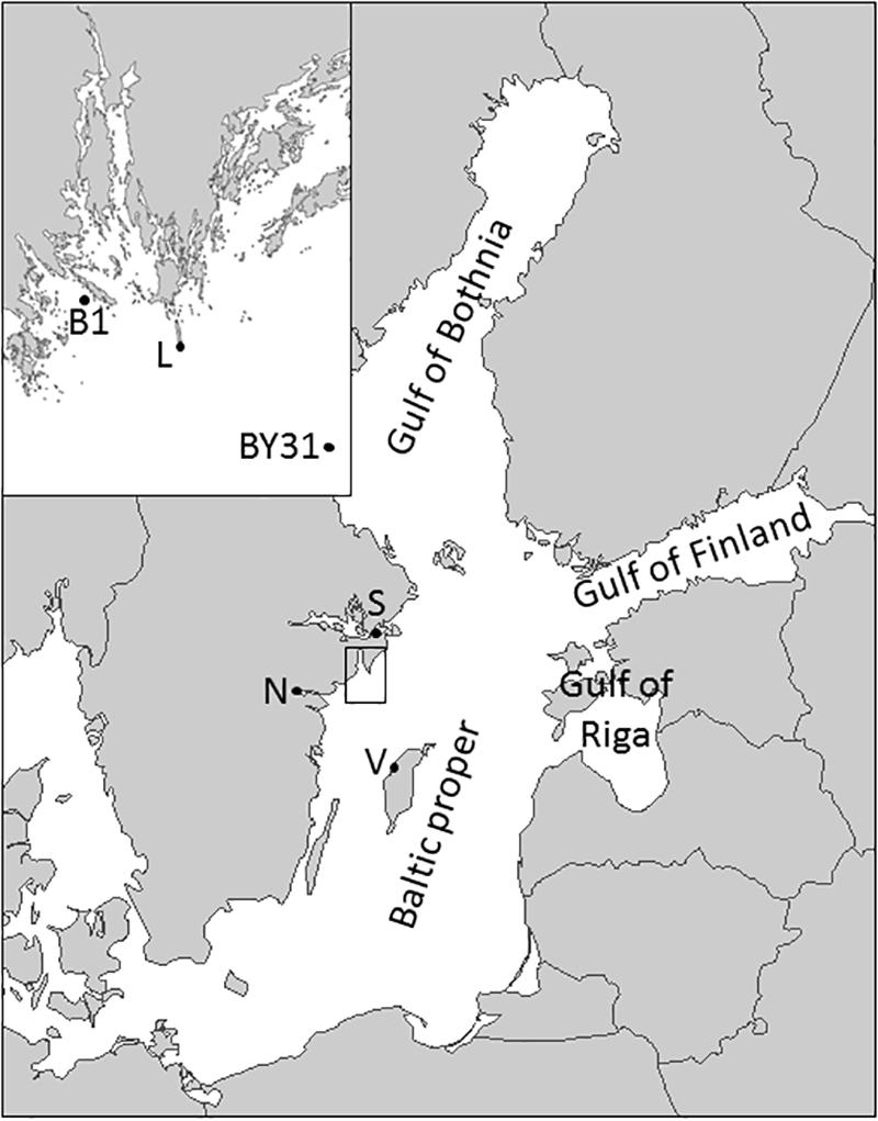
Figure 1. Map of the Baltic Sea and the study area, with the coastal (B1) and the offshore sampling station (BY31) as well as the SMHI weather stations in Visby (V), Norrköping (N), Stockholm (S) and Landsort (L) marked.
Phytoplankton Data
Samples were taken as integrated samples with a sampling hose (inner diameter 19 mm) from 0 to 20 m and preserved with acid Lugol’s solution. Phytoplankton (>2 μm) were counted after sedimentation in 10 to 50 mL chambers (between 1977 and 1982 even 5 mL) using an inverted microscope with phase contrast (10 to 40× objective), according to the (HELCOM, 2014) guidelines. Microphytoplankton were counted on the half or whole chamber bottom or in diagonals with a 10× objective (total magnification 150). Nanoplankton were counted in one or two diagonals (from 1977 to 1982 in 10 fields) with a 40× objective (total magnification 600×). In each sample, a minimum of 50 units (cells/colonies/filaments) of the dominating species were enumerated, giving a maximum counting error of ±28% corresponding to a 95% confidence limit for the counts (Lund et al., 1958); maximum error for total count per sample was less than ±10% (until 1992 only dominating species were counted giving about 10% lower total biomass). Biomass (carbon content) was estimated by multiplying the cell numbers with species specific, size classed, cell volumes using the recommendations by Olenina et al. (2006) and the related standard volumes1. Daily carbon content (μg C L–1) of auto- and mixotrophic species was estimated by daily linear interpolation between sampling dates for four major taxonomic spring groups: diatoms, dinoflagellates, M. rubrum and others.
The timing (T) of the bloom is represented by the center of gravity (COG, Edwards and Richardson, 2004; Meis et al., 2009) of the carbon content (C, per taxon group or total biomass) within the period March–May (day 60–120, d), the time period when spring blooms typically occur (see Figure 2):
FIGURE 2
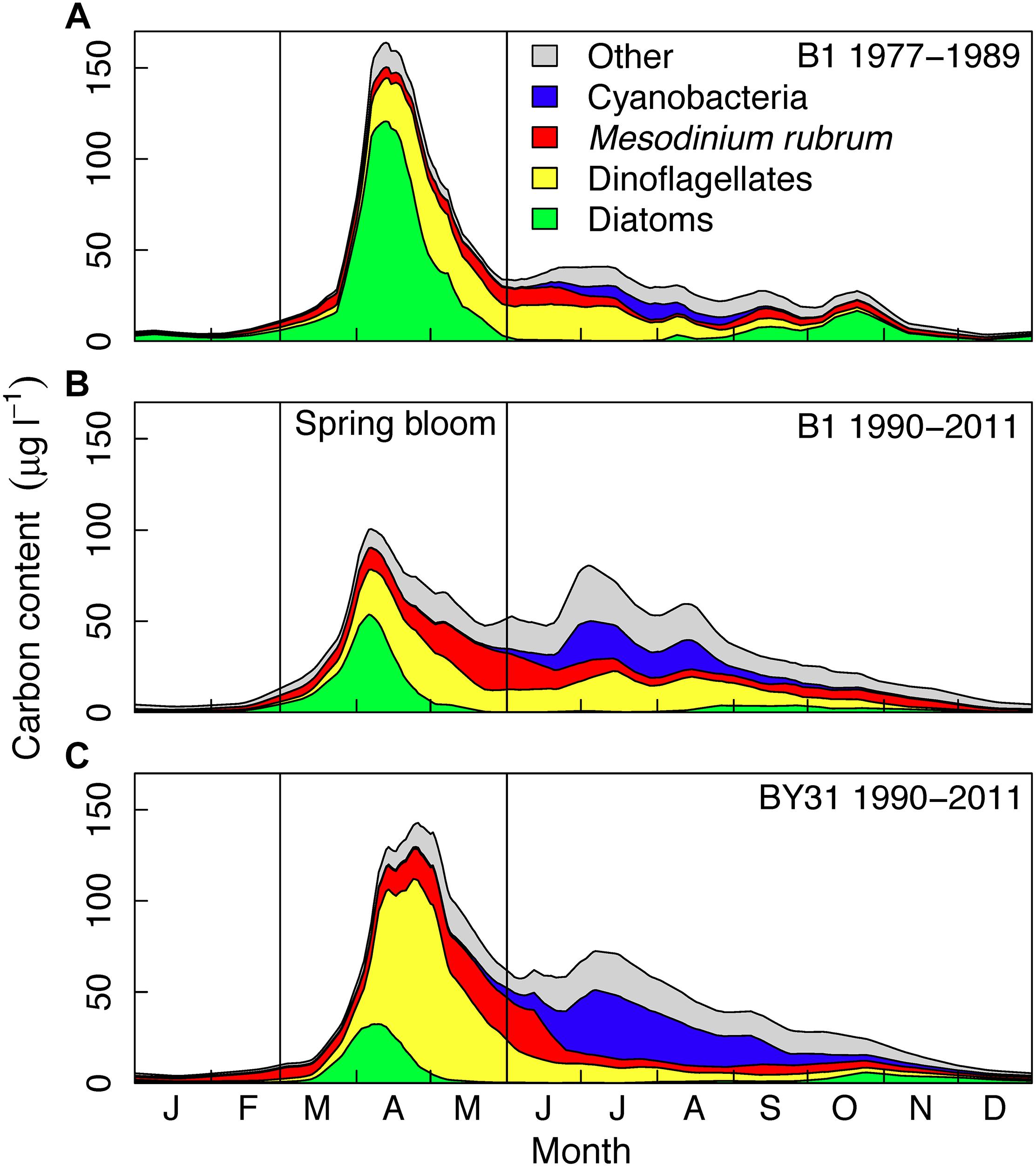
Figure 2. Average long-term seasonal biomass dynamics at the Baltic Sea coastal (A,B, B1) and offshore (C, BY31) station of major phytoplankton taxonomic groups in the northern Baltic Proper. The B1 time series is split into two time periods: (A) 1977–1989 and (B) 1990–2011, the latter period overlapping with the BY31 time series (C). Years 1992–1993 was removed at both stations due to incomplete sampling. The vertical lines indicate the spring period (March–May) investigated in this study.
Consequently, an early bloom does not only relate to an early start of the bloom, but is also dependent on how soon the bloom peak and termination occur. One reason for using the COG was that the bloom start would have been more difficult to determine due to small biomasses and sometimes low sampling frequency at the start of the bloom, but also that the COG better mirrors the feeding conditions for higher trophic levels. The magnitude of the bloom is the average of the daily total carbon content in March–May, and to describe the bloom composition we used the relative contribution by group in March–May (average daily carbon content per group/magnitude).
Hydrochemical Data
Temperature and salinity were measured with a CTD probe, and from discrete depths with 5 m intervals at station B1 before 1996. Missing observations were rare (1–2%) and replaced by linear interpolation first between depth and if needed between sampling date data points. Vertical profiles of water density were estimated from temperature, salinity and depth data (Gill, 1982) and the mixed layer depth (MLD) was defined as the depth where the density was 0.15 kg m–3 greater than at 1.5 m depth. For temperature, the average values of the upper 20 m were used. Dissolved inorganic nitrogen (DIN) was estimated as the sum of nitrate, nitrite and ammonium and were sampled every 5th meter. The maximum winter (January–March) concentration averaged over the upper 20 m were used in the analysis.
Climate Data
Monthly average wind speed (m s–2) was estimated from observations every third hour at station Landsort (until 1995) and Landsort A (from 1996, 58°74′N, 17°87′E) by the Swedish Meteorological and Hydrological Institute (SMHI2, Figure 1).
Since photosynthetically active radiance (PAR) measurements were not available for the entire time periods, we used SMHI hourly data of global irradiance (Wh m2) as a proxy for PAR. Based on geographical distance and land-offshore characteristics, we used observations from Stockholm (59°35′N, 18°07′E) and Visby (57°67′N, 18°35′E, Figure 1) at the Island of Gotland to represent the coastal station B1 and the offshore station (BY31), respectively. Missing night observations were replaced by zeroes and missing day observations (max 7/day) were estimated by multiplying the average of the two closest surrounding non-missing observations by the ratio of the missing and the surrounding non-missing observations of the three closest dates in the entire dataset (all years). Daily average global irradiance was calculated and days with missing observations (2% of the days) were estimated based on major axis model II regression (R package lmodel2, version 1.7-0) (Legendre, 2011) between the station with missing observations and station of Stockholm, Visby and Norrköping (58°58′N, 16°15′E) with the best fit for the corresponding dates of the other years. Finally, missing daily values for 1–15 March 1980 in Stockholm (no observations from the other two stations were available) was estimated based on linear regression between daily global irradiance anomalies from a five day moving average and the cloudiness index (1–9) from SMHI’s climate observations at station Landsort in March.
Ice codes from SMHI’s ice cover maps3, observed and published twice a week since 1981, were visually translated into an ice cover index (1 = intact and close ice, 0.5 = open ice, 0 = open water). After daily linear interpolation of those indices between observation days, the number of ice days per winter was estimated as the sum of the daily ice cover indices. The number of ice days at B1 before 1981 was based on SMHI’s fairway ice codes for the closest fairway section, named Fifong-V Röko.
Statistical Analysis
The non-parametric Mann–Kendall test was used to investigate monotonic trends in spring bloom dynamics and environmental variables (R package wq, version 0.4-1, (Jassby and Cloern, 2014). At the coastal station the trend was estimated for both the full time series (1977–2011) and from 1990 to 2011 to be comparable to the time series at the offshore station (BY31). We used a multiple linear regression analysis to evaluate the ability of environmental variables to explain the spring bloom dynamics. Response variables were non-transformed (timing), logit transformed (relative contribution) and log-transformed (magnitude) to fulfill model assumptions of homogenous variance. Due to high correlations of the residuals between stations within years, we analyzed the two stations separately.
As predictor variables for the analysis of timing and relative contribution we used average water temperature, wind speed, global irradiance and MLD in March and the number of ice days. In the analysis of the relative contribution by taxonomic group, we also used the maximum winter DIN and winter (December–February) wind speed, but since winter and March wind speed were correlated they were not used simultaneously in the same model. For the magnitude, we assumed that the conditions during, rather than before, the bloom peak were more relevant given their fast growth and rapid turnover and therefore the temperature, global irradiance and MLD in April were used. Collinearity of predictors was tested by VIF (variance inflation) analysis and predictors with VIF values >3 were removed from the analysis, i.e., ice and wind (at BY31) in the analysis of bloom magnitude (the R package car, Fox and Weisberg, 2011).
We fitted models with selected predictor variables motivated by plausible ecological mechanisms using the dredge function in the R package MuMIn (Barton, 2014). AIC values corrected for finite sample sizes (AICc) and AICc weights, the probability that a model is the best model (Burnham and Anderson, 2002) were used to select the best models corresponding to the 95% cumulative AICc weights. From these selected models, we calculated an AICc weighted average model (i.e., a model with a high AICc weight had a larger effect on the average model) and AICc weighted slopes, p-values and R2-values (wR2).
Model validations in terms of residual plots were used to visually check for non-linear patterns, homogeneity of variances, normality, influential outliers, and temporal autocorrelation. No major violations of the assumptions were detected and minor violations are indicated in the corresponding model results (p and wR2-values) and should be interpreted with care.
Results
Seasonal, Successional and Coastal-Offshore Patterns
Long-term averages show a pronounced phytoplankton spring bloom in the Baltic Sea with a large biomass in relation to the summer (June–August) biomass (Figure 2). At the coastal station B1, the average of the spring bloom was about twice as large than the summer biomass during 1977–1989 (Figure 2A) and slightly higher than the summer bloom during 1990–2011 (Figure 2B), which corresponds to the sampling period of BY31. At the offshore station BY31, average spring bloom biomass was about 30% larger than the summer biomass over the sampling period 1990 to 2011 (Figure 2C). The spring bloom at both stations generally started with a diatom bloom, followed by dinoflagellates. Diatoms dominated the bloom at B1 before 1990 (about half of the average biomass in March–May). From 1990 onward dinoflagellates and diatoms where on average equally important at B1 (about one third each) and dinoflagellates dominated (more than half of the biomass) at BY31. The proportion of M. rubrum was similar at the two stations (20–25% of the biomass after 1990) and often had a later and less distinct biomass peak than diatoms and dinoflagellates.
Patterns and Trends in Spring Bloom Timing, Composition and Magnitude
Bloom timing, composition and magnitude displayed considerable inter-annual variability and, except for magnitude, temporal trends (Figure 3). The timing (center of gravity) of the spring bloom total biomass was on average in mid/late April (day 111 ± 6 days standard deviation) at the coastal station. The diatom bloom was on average 11 days before (±6 days) and the dinoflagellate bloom was 6 days after (±6 days) the timing of the total biomass (Figures 3A–C). The bloom at the offshore station occurred on average 6 days later than at B1 (p < 0.001, paired t-test) and this is supported by taxon-specific bloom timing in relation to the coastal station (diatoms, ++4 days, p = 0.01 and dinoflagellates, +3 days, p = 0.03) (Figures 3A–C). In 1990–2011 there were trends of earlier blooms of diatoms at both stations and dinoflagellates at B1 by about 5 days decade–1, and similar but weaker trends for the total biomass. The proportion of diatoms at B1 decreased over the entire sampling period (p = 0.03) and was high until 1988, dropped quickly in 1989 and remained after 1990 at relatively low and stable levels at both stations (Figure 3D). The proportion of dinoflagellates decreased significantly from about 60 to 40% of total phytoplankton biomass between 1990 and 2011 at BY31 (11%⋅decade–1), though no consistent trend was observed at B1 (Figure 3E). Proportions of M. rubrum showed opposite trends to that of diatoms at B1, with low values until 1988, high around 1990 (∼50% of the biomass) and a significant negative trend after 1990 (10%⋅decade–1) (Figure 3F).
FIGURE 3
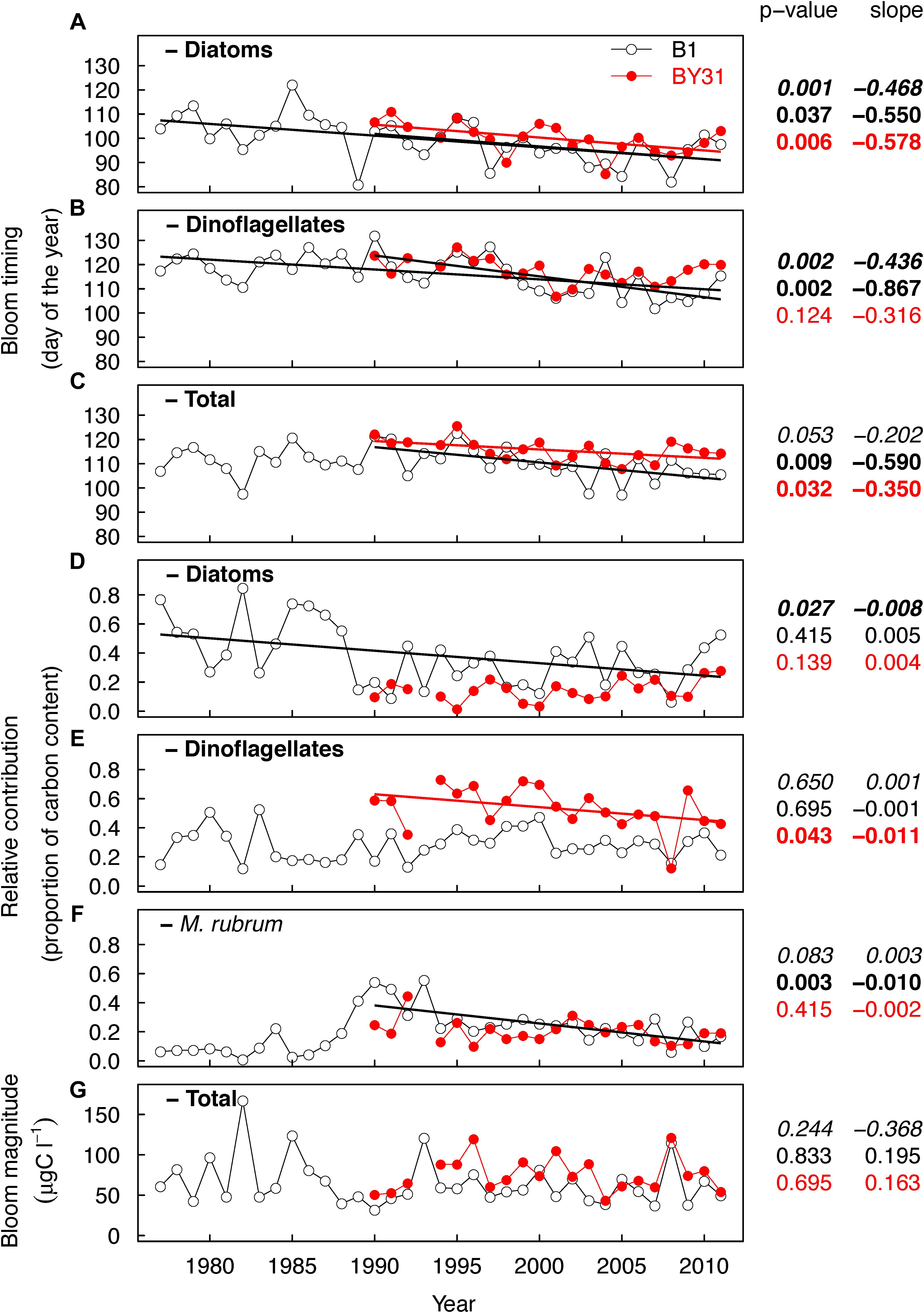
Figure 3. Temporal trends in phytoplankton bloom timing (A–C), contribution of major taxa to spring bloom (D–F) and bloom magnitude (G) at the coastal (B1, open circles, black lines) and offshore (BY31, red) station in the northern Baltic Proper. Spring bloom timing is shown for diatoms (A), dinoflagellates (B) and total phytoplankton biomass (C), and the relative contribution to the spring bloom biomass for diatoms (D), dinoflagellates (E) and Mesodinium rubrum (F), and total phytoplankton for spring bloom magnitude (G). The p-values and Theil–Sen slopes are from the non-parametric Mann–Kendall analysis. Bold font = significant trends, first line (italics font) = B1 trends for the full time period 1977–2011 and since 1990 (second line, regular font), third line (red text) = BY31. The regression lines in the plots are visualizations of significant trends based on linear regression.
Patterns and Trends in Environmental Variables
March water temperature at the coastal station (B1) was always below 1°C until 1988 and increased stepwise in 1989 (Figure 4A). After 1990 the temperature was on average higher compared to the time period before (up to >3°C) and more variable at both stations, without any monotonic trend. Interannual temperature variability followed a similar pattern at both stations. Ice conditions showed a corresponding pattern with several strong ice winters (almost 100 days of ice cover) at B1 before 1988 and few winters with ice since then at both stations (Figure 4B). The average wind speed in March decreased significantly, especially after 1990 (0.08 m s–1 year–1) (Figure 4C). The March MLD showed an increasing trend from about 14 to 22 m in 1977–2011 at B1 (0.25 m year–1), with no trend at neither station after 1990 (Figure 4D). We found close to significant increasing trends in light intensity after 1990 (1 Wh m2) (Figure 4E). Maximum winter DIN concentrations decreased after 1977 at B1 and 1990 at B1 and BY31 (Figure 4F). April temperature, wind speed and global irradiance, which were used in the regression analysis of bloom magnitude, showed similar patterns as in March (data not shown).
FIGURE 4
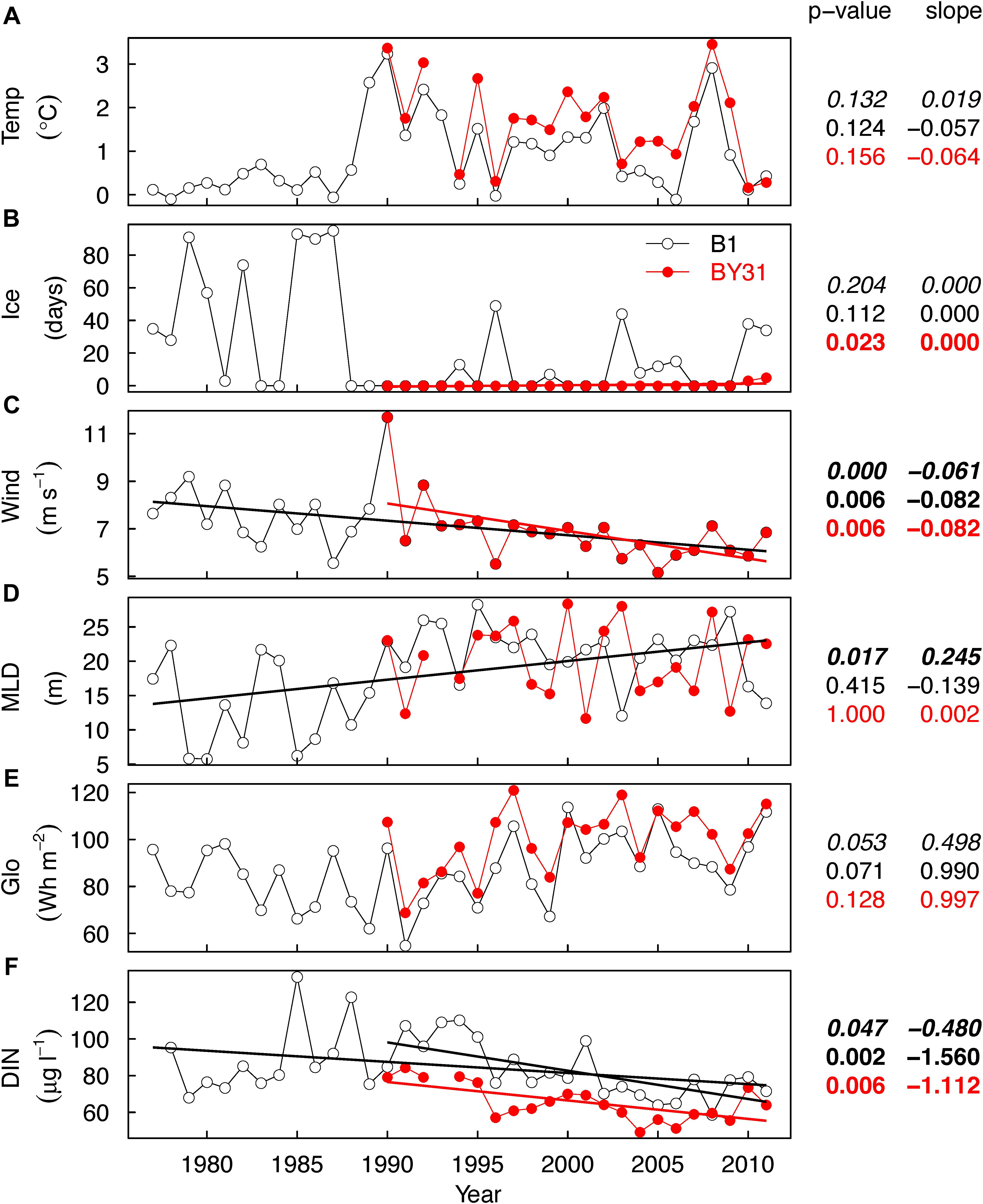
Figure 4. Temporal trends in average March water temperature in 0–20 m, Temp (A), the number of ice days, Ice (B), average wind speed in March, Wind (C), mixed layer depth in March, MLD (D), Global irradiance in March, Glo (E) and maximum winter concentration of dissolved inorganic nitrogen, DIN (F) at the coastal (B1, open circles, black lines) and offshore (BY31, red) stations in the northern Baltic Proper. The p-values and Theil–Sen slopes are from the non-parametric Mann–Kendall analysis. Bold font = significant trends, first line (italics font) = B1 trends for the full time period 1977–2011 and since 1990 (second line, regular font), and third line (red text) = BY31. The regression lines in the plots are visualizations of significant trends based on simple linear regression.
Drivers of Bloom Timing
A substantial proportion of the variation in bloom timing of diatoms, dinoflagellates and total biomass at both stations was explained by the multivariate models (32–74%, Figure 5), except for diatoms at the offshore station (BY31, 7%). In general, calm (low wind) and sunny spring conditions were associated with early blooms of total phytoplankton biomass at both stations as well as diatoms at B1 and dinoflagellates at BY31. Offshore (BY31), bloom timing of the total biomass and dinoflagellates correlated positively to the MLD, i.e., a shallow MLD were associated with earlier blooms. Temperature was negatively correlated to bloom timing (high temperatures = earlier blooms) of diatoms at the coastal station B1 and dinoflagellates at both stations, but did not affect timing of the total biomass. Ice cover had no effect on any phytoplankton bloom timing at both stations.
FIGURE 5
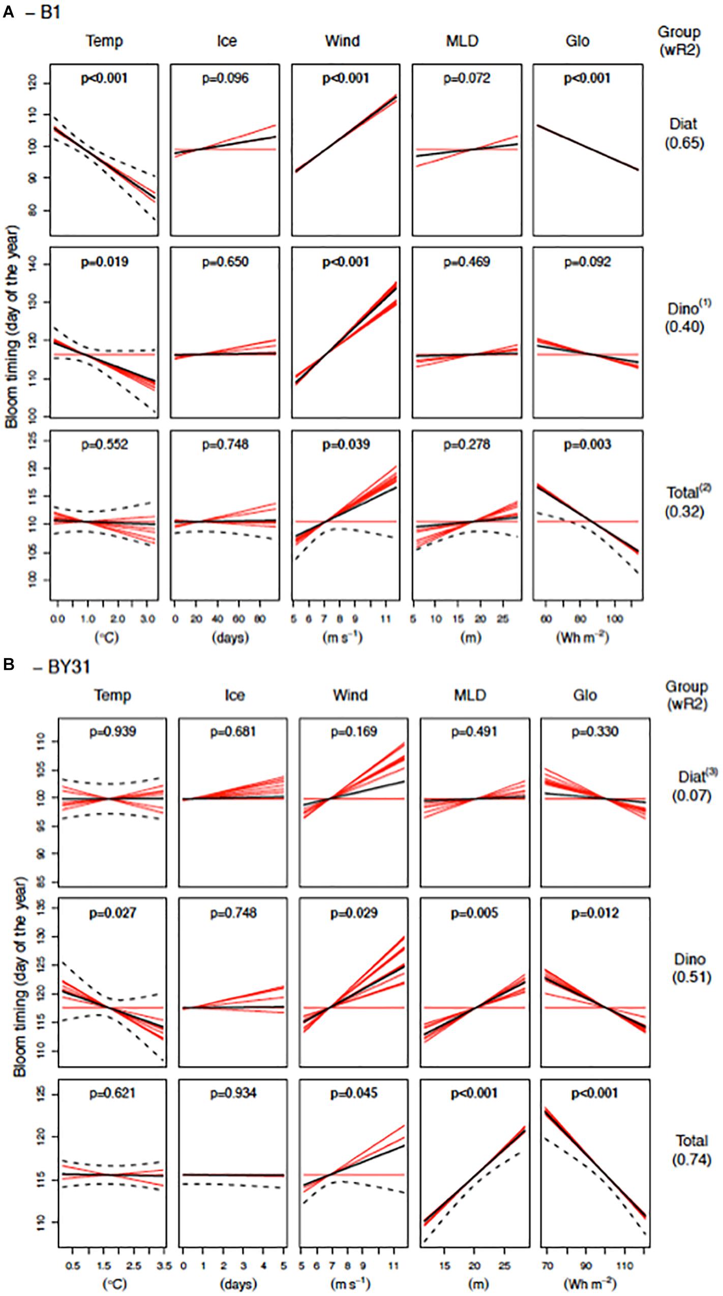
Figure 5. Regression analysis results of spring bloom timing (biomass center of gravity in March–May) of diatoms, dinoflagellates and total biomass at the coastal station (A, B1) and the offshore station (B, BY31) in the northern Baltic Proper. The solid and dashed black lines are the fitted regression lines and the 95% confidence intervals of the average models, respectively. Red lines are the fitted regression lines of the individual models that contribute to the average model. If the slopes of a predictor are either all positive or negative in the individual models there is strong support for an effect of the predictor, while different signs or lack of slope indicate uncertainty of its effect. The black circles represent the partial residuals from the average model. p-values within the panels and the weighted R2 (wR2) values are based on the AICc weights. Model results should be interpreted with care when model validation plots indicate violation to the model assumptions: (1) Model residuals slightly non-linear vs. fitted values, (2) Significant negative temporal autocorrelation at lag 1, (3) Model residuals have a u-shaped relationship to light (Glo), indicating a non-linear relationship would be better.
Drivers of Bloom Composition
The models explained about half of the variation (42–55%) in the proportion of diatoms at both stations and M. rubrum at B1, but less for dinoflagellates at both stations and M. rubrum at BY31 (12–0.25%, Figure 6). At the coastal station, the relative proportion of diatoms was most strongly related to long ice winters with a corresponding tendency of a negative correlation to March water temperatures. At the offshore station, diatoms were also most common during the only two ice winters, but were mainly related to a shallow MLD and a high light intensity. For dinoflagellates no strong predictors were evident, and were strongest correlated to water temperatures and, seemingly contradictory, to the number of days with ice cover. M. rubrum at B1 was, in contrast to diatoms, associated with short ice winters though no predictors significantly explained the proportion of M. rubrum at BY31. March and winter wind speed and the maximum winter concentration of DIN had no significant effects on any phytoplankton group (not shown).
FIGURE 6
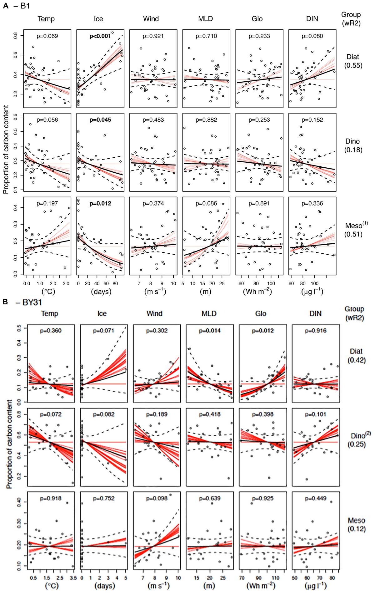
Figure 6. Regression analysis results of group composition (the relative contribution of diatoms, dinoflagellates and Mesodinium rubrum to the average biomass in March–May) at the coastal station (A, B1) and offshore station (B, BY31) in the northern Baltic Proper. The solid and dashed black lines are the fitted regression lines and the 95% confidence intervals of the average models, respectively. Red lines are the fitted regression lines of the individual models that contribute to the average model. If the slopes of a predictor are either all positive or negative in the individual models there is strong support for an effect of the predictor, while different signs or lack of slope indicate uncertainty of its effect. The black circles represent the partial residuals from the average model. p-values within the panels and the weighted R2 (wR2) values are based on the AICc weights. Model results should be interpreted with care when model validation plots indicate violation to the model assumptions: (1) Possibly slightly non-normal distribution of residuals (long lower tail), (2) Just significant negative temporal autocorrelation at lag 3 and higher variance of residuals at low fitted values.
Drivers of Bloom Magnitude
The models only explained a small proportion (B1 29%, BY31 10%) of the variation in bloom magnitude of total biomass (Figure 7). Neither water temperature, light (Glo), nor maximum winter DIN in the upper 20 m seemed to have any effect on the bloom magnitude. At B1, shallow mixed layers and low wind speed were associated with large blooms and no predictors were significant at BY31.
FIGURE 7
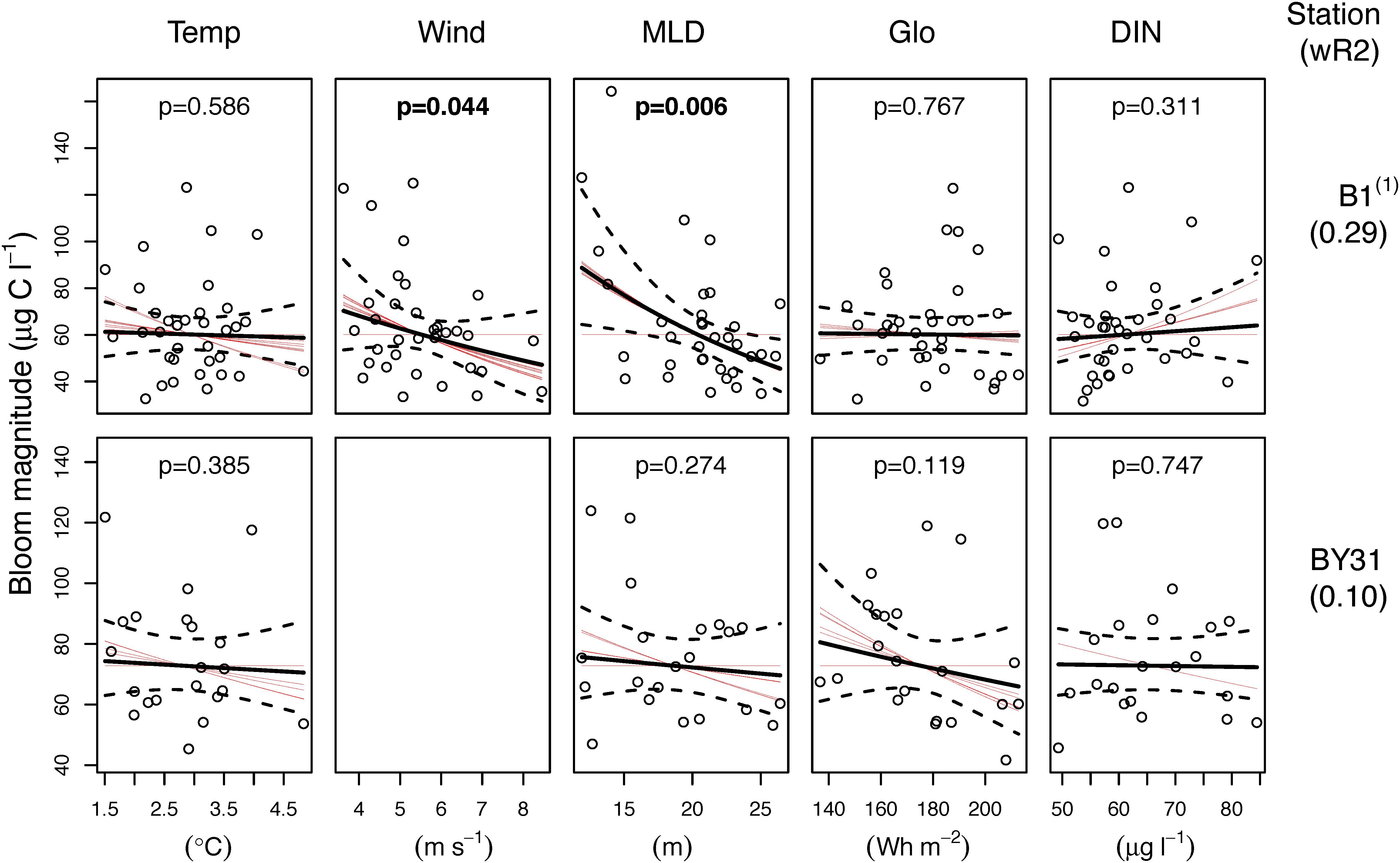
Figure 7. Regression analysis results of spring bloom magnitude (average total biomass in March–May) at the coastal station (B1, upper panels) and the offshore station (BY31, lower panels) in the northern Baltic Proper. The solid and dashed black lines are the fitted regression lines and the 95% confidence intervals of the average models, respectively. Red lines are the fitted regression lines of the individual models (within the 95% cumulative weighted AICc values) that contribute to the average model. If the slopes of a predictor are either all positive or negative there is strong support for an effect of the predictor, while different signs or lack of slope indicate uncertainty of its effect. The black circles represent the partial residuals from the average model. p-values within the panels and the wR2 values are based on the AICc weights. Model results should be interpreted with care when model validation plots indicate violation to the model assumptions: (1) Just significant negative temporal autocorrelation at lag 1.
Discussion
In this study we investigated how a variable climate influences the spring bloom, which is one of the main energy sources to the Baltic Sea’s food web. Though climate change associated trends in environmental variables were only weakly discernible, environmental factors showed sufficient variability to investigate their effects on phytoplankton spring blooms. Our results show that the trend toward earlier spring blooms was likely caused by more sunshine and less windy conditions. High temperatures were associated with earlier blooms of diatoms and dinoflagellates, but since mild and short ice winters changed the bloom composition toward later blooming species no temperature effect on overall bloom timing was detected.
Bloom Timing
Earlier spring blooms have been reported for the northern Baltic Proper before (Fleming and Kaitala, 2006; Klais et al., 2013; Lips et al., 2014) and our study showed that total phytoplankton spring bloom appear earlier by 1–2 weeks in the northern Baltic Proper from 1990 to 2011 (Figure 3). We found no evidence that this trend was caused by a warming climate as suggested before (Fleming and Kaitala, 2006; Klais et al., 2013; Lips et al., 2014). In fact, after a stepwise increase of water temperature in the upper 20 m in 1989, the average spring (March and April) water temperature remained unchanged after 1990 (Figure 4A). The sudden increase in water temperature is in line with a regime shift in the Central Baltic Sea in the late 1980s as observed by abrupt changes in hydroclimatic and biological variables as a result of changing atmospheric forcing (Möllmann et al., 2009). Instead less wind, increasing light intensity and reduced MLD at the offshore station seemed to explain the earlier blooms. Positive effects of low wind speeds (c.f. the critical turbulence hypothesis) and high light intensity on spring bloom development is supported by observations, modeling studies and theories (Townsend et al., 1992; Huisman et al., 1999, 2002; Collins et al., 2009; Nixon et al., 2009; Sommer et al., 2012), but has not been shown in Baltic Sea field data before. In agreement with the critical depth hypothesis (Sverdrup, 1953) we found a positive correlation between the MLD and the total phytoplankton bloom timing (i.e., shallow MLD = earlier bloom) at the offshore station (BY31), but not at the coastal station. This difference between the stations is reasonable since stratification is generally more important for bloom initiation in deep offshore areas than in shallow coastal areas where the maximum MLD is set by water depth (Townsend et al., 1994; Sommer and Lengfellner, 2008).
Temperature changes could not explain the observed trend toward earlier blooms of total phytoplankton, but high water temperature was associated with early blooms of both diatoms at B1 and dinoflagellates at both stations. Mechanistically, higher temperature is often thought to induce earlier blooms by causing thermal stratification, which results in high light intensities in a shallow mixed layer (c.f. the critical depth hypothesis and (Sommer et al., 2012). This is, however, not a likely explanation for the northern Baltic Proper since the bloom often starts before thermal stratification develops and stratification by freshwater inflow (snow or ice melt) is here considered more important (Kahru and Nommann, 1990; Höglander et al., 2004; Stipa, 2004). It is noteworthy that despite a correlation between water temperature and bloom timing of those dominating taxa, temperature had no effect on the timing of the total phytoplankton spring bloom. This seemingly contradictory result is probably explained by a shift from early blooming diatoms to later blooming M. rubrum and to some extent dinoflagellates at higher temperatures that buffer the effect on bloom timing (discussed below).
Bloom Composition
The spring bloom composition at both stations showed a general successional pattern observed in the Baltic Proper and Gulf of Riga (e.g., Jurgensone et al., 2011; Klais et al., 2011), starting with diatoms followed by dinoflagellates, while M. rubrum were present throughout the bloom and had a less distinct and later peak. The proportion of dinoflagellates was higher at the offshore station (BY31) and the proportion of diatoms was lower compared to at the coastal station (B1). Although we only analyzed one coastal and one offshore station, this probably reflects a general coastal vs. offshore pattern observed in the Baltic Proper (Wasmund et al., 2013). Bloom initiation for both diatoms and dinoflagellates depends on resuspension of resting stages, most likely from shallow coastal areas, but motile dinoflagellates are probably more likely to stay buoyant longer and reach deep offshore areas by horizontal transportation than faster sedimenting diatoms. Dinoflagellates should also be more able than diatoms to utilize the larger nutrient pool down to the halocline (∼60 m) in deeper offshore areas (Höglander et al., 2004).
The proportion of diatoms was high at the coastal station (B1) until 1988, dropped suddenly in 1989 and remained at a relatively low level after 1990 at both stations. This pattern of a sudden shift agrees reasonably with findings in the central and southern Baltic Proper (Wasmund et al., 1998, 2013; Wasmund and Uhlig, 2003). We detected a strong association between long ice winters and a high proportion of diatoms at B1, and a tendency that low temperature was related to more diatoms (Figure 6). We conclude that diatoms are favored after cold and icy winters, but our results indicate that ice directly rather than temperature was more important to diatoms in this area. A likely mechanistic explanation is that ice provides a habitat for diatom species like Achnantes teaniata, Melosira arctica, Nitzschia frigida, Navicula vanhoeffenii and Chaetoceros wighamii that can grow in or attached under the ice (Norrman and Andersson, 1994; Haecky et al., 1998) that results in a large seed population after ice break-up. However, even in mainly ice-free areas of the southern Baltic Sea a relationship between low temperatures and diatoms has been observed (Wasmund et al., 2013). Different hypotheses have been proposed to explain effects of temperature. Decreased convective mixing during mild winters could favor motile dinoflagellates (and M. rubrum) over diatoms since diatoms need stronger mixing for the resuspension of resting stages and to stay buoyant in the photic layer (stratification hypothesis, Wasmund et al., 1998, 2013; Wasmund and Uhlig, 2003; Alheit et al., 2005). Alternatively, higher zooplankton survival during mild winters could result in a larger grazing pressure on diatoms (grazing hypothesis, Sommer and Lewandowska, 2011; Wasmund et al., 2011, 2013). However, given that spring bloom dinoflagellates are a high-quality food for copepods (Vehmaa et al., 2011), high grazing pressure should also affect dinoflagellate biomass and a selective grazing impact on phytoplankton species composition remains to be shown experimentally. Though not sufficiently frequent to produce a marked pattern, we also observed at the offshore station (BY31) that the 2 years with the highest proportion of diatoms followed the only two ice winters (2010 and 2011, Figures 3, 4). Temperature had no effect, but instead a shallow mixed layer and high light intensities, i.e., conditions related to early blooms at this station, were associated with high proportions of diatoms. This was somewhat surprising since diatoms are considered favored by more mixing in relation to dinoflagellates (Wasmund et al., 1998, 2013).
Earlier studies (Jurgensone et al., 2011; Klais et al., 2011; Wasmund et al., 2011) have observed an increasing spring biomass or proportion of dinoflagellates in the Baltic Sea until the mid-1990s, but we did not find any trends in the proportion of dinoflagellates at the coastal station (B1). However, at the offshore station we found a negative trend in the proportion of dinoflagellates in agreement with observations in the southern Baltic Proper (Wasmund et al., 2011) and the Gulf of Riga (Jurgensone et al., 2011), but in contrast to the Gulf of Finland and the Gulf of Bothnia (Klais et al., 2011).
We found no strong correlations between dinoflagellate proportions and environmental variables. There was a contradicting tendency that short ice winters, but also low water temperatures were related to high proportions of dinoflagellates. This might indicate that dinoflagellates have a non-linear dome-shaped relationship to temperature, where intermediate temperatures would favor dinoflagellates. Klais et al. (2013) found a similar relationship where a high proportion of dinoflagellates were correlated to medium ice thickness, but interestingly we found no support for such a relationship to ice specifically in our results. While our sites were included in the (Klais et al., 2013) study their analysis was dominated by Gulf of Finland data and their results may primarily reflect the climate conditions of that area. Klais et al. (2013) also found an association between high winter wind speeds and dinoflagellates and suggest that strong pre-ice winds favor dinoflagellates by resuspension of resting cysts (Klais et al., 2011), but we found no effect either of winter (data not shown in Figure 6) or March wind speed at our stations. We conclude that spatial differences in bloom dynamics should be expected in an area like the Baltic Sea with several environmental latitudinal, longitudinal and coastal offshore gradients and it is a challenge to science that calls for both detailed local as well as more general regional studies and management.
The autotrophic ciliate M. rubrum is not a strict spring bloom species and its contribution to the spring bloom is not as well investigated as that of diatoms and dinoflagellates. At the offshore station (BY31) we found no temporal trend and no strong effects of environmental conditions on M. rubrum. At the coastal station (B1) the temporal development of the M. rubrum proportion was opposite to that of diatoms and was negatively correlated to ice cover. This could be a direct effect by ice (or temperature) or an indirect effect by competition with ice favored diatoms. M. rubrum has a high swimming speed of up to 8 mm s–1 (Lindholm, 1985) and is able to collect nutrients from larger depths by vertical migration (Crawford, 1989; Passow, 1991). This could be an advantage in mild winters when thermal stratification starts earlier and limits up-mixing of nutrients. However, we found no association between M. rubrum and a shallow MLD (rather a tendency of the opposite at B1), indicating that the motile M. rubrum does not seem dependent on stratified conditions during the early spring bloom to be competitive. M. rubrum also has a jumping behavior that enables it to avoid predation (Jonsson and Tiselius, 1990; Fenchel and Juel Hansen, 2006), which can give it a competitive advantage if mild winters lead to higher grazing pressure (c.f. Sommer and Lengfellner, 2008; Winder et al., 2012).
Our study suggests that temperature related shifts in phytoplankton species composition toward later blooming taxa counteract the effect of climate related shifts toward earlier bloom timing of total phytoplankton spring biomass. A similar mechanisms but opposite direction of spring bloom timing was observed in Lake Washington (Walters et al., 2013), where a change in composition toward early blooming taxa has driven the large shift toward earlier timing of the aggregate community spring-summer phytoplankton peak, despite an average small taxon-specific shifts in peak timing. This highlights the importance of both general and taxon-specific investigations of phytoplankton response to environmental variation for the mechanistic understanding and possibilities to forecast effects of climate change.
Bloom Magnitude
In the northern Baltic Sea, phytoplankton spring bloom declined, while summer blooms increased (HELCOM, 2013). In comparison we found no consistent trends in spring bloom magnitude of total phytoplankton but a change in the relative composition of phytoplankton taxa. However, the long-term phytoplankton spring average was lower compared to the summer phytoplankton biomass after 1989 in B1 (Figure 1), which was strongly driven by few years with high spring bloom biomass between 1977 and 1989. Despite that the spring bloom in the Baltic Proper is nitrogen limited (Granéli et al., 1990), we did not find any positive effect on bloom magnitude by winter concentrations of DIN. Most likely spring primary production will depend on nitrogen uptake down to the bottom (coastal area) or permanent halocline (open sea), but vertically homogenous winter DIN concentrations in the upper 20 m motivates the use of surface concentrations. The average carbon content in the upper 20 m in March–May might underestimation bloom primary production due to losses through down-mixing, active migrating cells to deeper water layers, sedimentation and grazing, which will most likely vary between years due to climate factors. The only environmental conditions associated with a large bloom magnitude were shallow MLD and a barely significant negative effect of wind speed at the coastal station. A shallow mixed layer and low wind speeds likely favors high primary production rates and biomass accumulation through decreased down-mixing of phytoplankton to darker conditions and concentration of phytoplankton biomass in the upper water column.
Response to Climate Change
Our results show that not only temperature but also other climate related environmental factors are important to understand and to predict ecological responses to climate change. The less windy and less cloudy springs observed after 1990 are linked to a negative trend in the North Atlantic Oscillation Index (p = 0.01, Mann–Kendall) and is most likely only a temporary shift in the long-term climate development. Climate models predict higher temperatures in the Baltic Sea and, although with a higher uncertainty, more precipitation (cloudiness) and an increase in windiness is somewhat more likely than a decrease (HELCOM, 2013; BACC Author Team, 2015). Extrapolating our results to a future with higher temperatures and less ice, we would expect decreased diatom bloom magnitudes as well as earlier blooms of diatoms and dinoflagellates, but a shift in composition to later blooming groups (e.g., M. rubrum) would buffer the effect on the overall bloom timing. Further, we expect the predicted trend toward earlier blooms of diatoms and dinoflagellates to be counteracted if the future becomes more cloudy and windy, thus also influencing the overall bloom timing. We emphasize that a simple response, such as earlier spring blooms, can be the product of complex processes, and that these processes need to be investigated jointly to understand the mechanisms underlying change in phytoplankton dynamics.
Conclusion
We hypothesize that future climate change could decrease the spring bloom biomass input to the benthic system via sedimentation toward remineralization in the pelagic system for several reasons. First, higher temperatures can increase zooplankton metabolic rate and/or winter survival, and therefore lead to higher grazing pressure (Winder et al., 2012). Second, a shift from early blooming diatoms to later blooming M. rubrum could decrease sedimentation rates and the energy input to the benthic system. Third, if climate becomes more cloudy and windy this could effectively delay the spring bloom, and thus increase the phytoplankton-zooplankton overlap period. A lower energy input to the benthic system would reasonably reduce benthic production above the halocline, but cause less pressure on benthic oxygen consumption and potentially decreasing anoxic zones (Spilling et al., 2018). However, higher water temperatures have been suggested to increase the oxygen consumption and anoxia below the halocline (Kabel et al., 2012; Meier et al., 2012). A reduced sedimentation due to changes in spring bloom composition could at least partly counteract this effect and influence biogeochemical processes with consequences on nutrient dynamics and ecosystem production (c.f. Fulweiler and Nixon, 2009).
Data Availability
The datasets generated for this study are available on request to the corresponding author.
Author Contributions
OH and MW designed the study and wrote a draft of the manuscript with input of the other co-authors. SH analyzed the phytoplankton samples. OH analyzed the data. OH, SH, UL, and MW interpreted the data. All authors read and significantly contributed to the manuscript.
Funding
This study was financially supported by Stockholm University’s Strategic Marine Environmental Research Program on Baltic Ecosystem Adaptive Management (BEAM) and received funding from the BONUS BIO-C3 project, and also supported by BONUS (Art 185), funded jointly by the EU and the Swedish Research Council FORMAS.
Conflict of Interest Statement
The authors declare that the research was conducted in the absence of any commercial or financial relationships that could be construed as a potential conflict of interest.
Acknowledgments
We thank all of those who have contributed to Stockholm University’s Baltic Sea monitoring program, especially Svante Nyberg for providing data and useful discussions and Marika Tirén for counting the phytoplankton samples. The use of the data from the National Swedish Monitoring Program, supported by the Swedish EPA, and supported by SMHI is gratefully acknowledged. We appreciate discussions and comments on the manuscript from Jennifer Griffiths and statistical advice by Johan Eklöf.
Footnotes
- ^ http://www.ices.dk/marine-data/vocabularies/Documents/PEG_BVOL.zip
- ^ www.smhi.se
- ^ http://www.smhi.se/klimatdata/oceanografi/havsis
References
Alheit, J., Mollmann, C., Dutz, J., Kornilovs, G., Loewe, P., Mohrholz, V., et al. (2005). Synchronous ecological regime shifts in the central Baltic and the North Sea in the late 1980s. ICES J. Mar. Sci. 62, 1205–1215. doi: 10.1016/j.icesjms.2005.04.024
BACC Author Team (2015). Second Assessment of Climate Change for the Baltic Sea Basin. Berlin: Springer.
Barton, K. (2014). MuMIn, Multi-Model Inference. R Package Version 1.10.5. Available at: http://CRAN.R-project.org/package=MuMIn
Behrenfeld, M. J. (2010). Abandoning Svedrup’s critical depth hypothesis on phytoplankton blooms. Ecology 91, 977–989. doi: 10.1890/09-1207.1
Behrenfeld, M. J., and Boss, E. S. (2014). Resurrecting the ecological underpinnings of ocean plankton blooms. Annu. Rev. Mar. Sci. 6, 167–194. doi: 10.1146/annurev-marine-052913-021325
Berger, S. A., Diehl, S., Stibor, H., Trommer, G., and Ruhenstroth, M. (2010). Water temperature and stratification depth independently shift cardinal events during plankton spring succession. Glob. Change Biol. 16, 1954–1965. doi: 10.1111/j.1365-2486.2009.02134.x
Berger, S. A., Diehl, S., Stibor, H., Trommer, G., Ruhenstroth, M., Wild, A., et al. (2006). Water temperature and mixing depth affect timing and magnitude of events during spring succession of the plankton. Oecologia 150, 643–654. doi: 10.1007/s00442-006-0550-9
Blomqvist, M., and Larsson, U. (1994). Detrital bedrock elements as tracers of settling resuspended particulate matter in a coastal area of the Baltic Sea. Limnol. Oceanogr. 39, 880–896. doi: 10.4319/lo.1994.39.4.0880
Burnham, K. P., and Anderson, D. R. (2002). Model Selection and Multimodel Inference: A Practical Information-Theoretic Approach, 2nd Edn. New York, NY: Springer.
Cederwall, H., and Elmgren, R. (1980). Biomass increase of benthic macrofauna demonstrates eutrophication of the Baltic Sea. Ophelia Suppl. 1, 287–304.
Collins, A. K., Allen, S. E., and Pawlowicz, R. (2009). The role of wind in determining the timing of the spring bloom in the Strait of Georgia. Can. J. Fish. Aquat. Sci. 66, 1597–1616. doi: 10.1139/f09-071
Crawford, D. W. (1989). Mesodinium rubrum: the phytoplankter that wasn’t. Mar. Ecol. Prog. Ser. 58, 161–174. doi: 10.3354/meps058161
Cushing, D. (1990). Plankton production and year-class strength in fish populations - an update of the match mismatch hypothesis. Adv. Mar. Biol. 26, 249–293. doi: 10.1016/s0065-2881(08)60202-3
Edwards, M., and Richardson, A. J. (2004). Impact of climate change on marine pelagic phenology and trophic mismatch. Nature 430, 881–884. doi: 10.1038/nature02808
Elmgren, R. (1989). Man’s impact on the ecosystem of the Baltic Sea: energy flows today and at the turn of the century. Ambio 6, 326–332.
Elmgren, R., and Larsson, U. (2001). “Eutrophication in the Baltic Sea area: integrated coastal management issues,” in Science and Integrated Coastal Management, eds B. V. Bodungen and R. K. Turner (Berlin: Dahlem University Press), 15–35.
Fenchel, T., and Juel Hansen, P. (2006). Motile behaviour of the bloom-forming ciliate Mesodinium rubrum. Mar. Biol. Res. 2, 33–40. doi: 10.1080/17451000600571044
Fleming, V., and Kaitala, S. (2006). Phytoplankton spring bloom intensity index for the Baltic Sea estimated for the years 1992 to 2004. Hydrobiologia 554, 57–65. doi: 10.1007/s10750-005-1006-7
Fox, J., and Weisberg, S. (2011). An {R} Companion to Applied Regression, 2nd Edn. Thousand Oaks CA: Sage.
Fulweiler, R. W., and Nixon, S. W. (2009). Responses of benthic–pelagic coupling to climate change in a temperate estuary. Hydrobiologia 629, 147–156. doi: 10.1007/978-90-481-3385-7_13
Gerten, D., and Adrian, R. (2002). Effects of climate warming, North Atlantic oscillation, and El Niño-Southern Oscillation on thermal conditions and plankton dynamics in Northern Hemispheric Lakes. Sci. World J. 2, 586–606. doi: 10.1100/tsw.2002.141
Granéli, E., Wallström, K., Larsson, U., Granéli, W., and Elmgren, R. (1990). Nutrient limitation of primary production in the Baltic Sea area. Ambio 19, 142–151.
Griffiths, J. R., Kadin, M., Nascimento, F. J. A., Tamelander, T., Törnroos, A., Bonaglia, S., et al. (2017). The importance of benthic–pelagic coupling for marine ecosystem functioning in a changing world. Glob. Change Biol. 23, 2179–2196. doi: 10.1111/gcb.13642
Haecky, P., Jonsson, S., and Andersson, A. (1998). Influence of sea ice on the composition of the spring phytoplankton bloom in the northern Baltic Sea. Polar Biol. 20, 1–8. doi: 10.1007/s003000050270
Hajdu, S. (2002). Phytoplankton of Baltic Environmental Gradients. Observations on Potentially Toxic Species. Ph.D. Thesis, Stockholm University: Stockholm.
Heiskanen, A., and Kononen, K. (1994). Sedimentation of vernal and late summer phytoplankton communities in the coastal Baltic Sea. Arch. Für. Hydrobiol. 131, 175–198.
HELCOM (2013). Climate Change in the Baltic Sea Area: HELCOM Thematic Assessment in 2013. Available at: http://www.helcom.fi/Lists/Publications/BSEP137.pdf
HELCOM (2014). Manual for Marine Monitoring in the COMBINE Programme of HELCOM. Available at: http://www.helcom.fi/Documents/Action%20areas/Monitoring%20and%20assessment/Manuals%20and%20Guidelines/Manual%20for%20Marine%20Monitoring%20in%20the%20COMBINE%20Programme%20of%20HELCOM.pdf
Höglander, H., Larsson, U., and Hajdu, S. (2004). Vertical distribution and settling of spring phytoplankton in the offshore NW Baltic Sea proper. Mar. Ecol. Prog. Ser. 283, 15–27. doi: 10.3354/meps283015
Huisman, J., Arrayás, M., Ebert, U., and Sommeijer, B. (2002). How do sinking phytoplankton species manage to persist? Am. Nat. 159, 245–254. doi: 10.1086/338511
Huisman, J., van Oostveen, P., and Weissing, F. J. (1999). Critical depth and critical turbulence: two different mechanisms for the development of phytoplankton blooms. Limnol. Oceanogr. 44, 1781–1787. doi: 10.4319/lo.1999.44.7.1781
Jassby, A. D., and Cloern, J. E. (2014). wq: Some Tools for Exploring Water Quality Monitoring Data. R package version 0.4-1.
Johansson, M., Gorokhova, E., and Larsson, U. (2004). Annual variability in ciliate community structure, potential prey and predators in the open northern Baltic Sea proper. J. Plankton Res. 26, 67–80. doi: 10.1093/plankt/fbg115
Jonsson, P., and Tiselius, P. (1990). Feeding-behavior, prey detection and capture efficiency of the copepod Acartia tonsa feeding on planktonic ciliates. Mar. Ecol. Prog. Ser. 60, 35–44. doi: 10.3354/meps060035
Jurgensone, I., Carstensen, J., Ikauniece, A., and Kalveka, B. (2011). Long-term changes and controlling factors of phytoplankton community in the Gulf of Riga (Baltic Sea). Estuar. Coasts 34, 1205–1219. doi: 10.1007/s12237-011-9402-x
Kabel, K., Moros, M., Porsche, C., Neumann, T., Adolphi, F., Andersen, T. J., et al. (2012). Impact of climate change on the Baltic Sea ecosystem over the past 1,000 years. Nat. Clim. Change 2, 871–874. doi: 10.1038/nclimate1595
Kahru, M., and Nommann, S. (1990). The phytoplankton spring bloom in the Baltic Sea in 1985, 1986 - multitude of spatiotemporal scales. Cont. Shelf Res. 10, 329–354. doi: 10.1016/0278-4343(90)90055-q
Klais, R., Tamminen, T., Kremp, A., Spilling, K., An, B. W., Hajdu, S., et al. (2013). Spring phytoplankton communities shaped by interannual weather variability and dispersal limitation: mechanisms of climate change effects on key coastal primary producers. Limnol. Oceanogr. 58, 753–762. doi: 10.4319/lo.2013.58.2.0753
Klais, R., Tamminen, T., Kremp, A., Spilling, K., and Olli, K. (2011). Decadal-scale changes of dinoflagellates and diatoms in the anomalous Baltic Sea spring bloom. PLoS One 6:e21567. doi: 10.1371/journal.pone.0021567
Legendre, P. (2011). lmodel2, Model II Regression. R Package Version 1.7-0. Available at: http://CRAN.R-project.org/package=lmodel2
Lignell, R., Heiskanen, A., Kuosa, H., Gundersen, K., Kuuppoleinikki, P., Pajuniemi, R., et al. (1993). Fate of a phytoplankton spring bloom - sedimentation and carbon flow in the planktonic food web in the Northern Baltic. Mar. Ecol. Prog. Ser. 94, 239–252. doi: 10.3354/meps094239
Lindholm, T. (1985). Mesodinium rubrum - a unique photosynthetic ciliate. Adv. Aquat. Microbiol. 3, 1–48.
Lips, I., Rünk, N., Kikas, V., Meerits, A., and Lips, U. (2014). High-resolution dynamics of the spring bloom in the Gulf of Finland of the Baltic Sea. J. Mar. Syst. 129, 135–149. doi: 10.1371/journal.pone.0021567
Lund, J. W. G., Kipling, C., and Le Cren, E. D. (1958). The inverted microscope method of estimating algal numbers and the statistical basis of estimations by counting. Hydrobiologia 11, 143–170. doi: 10.1007/bf00007865
Meier, H. E. M., Hordoir, R., Andersson, H. C., Dieterich, C., Eilola, K., Gustafsson, B. G., et al. (2012). Modeling the combined impact of changing climate and changing nutrient loads on the Baltic Sea environment in an ensemble of transient simulations for 1961–2099. Clim. Dyn. 39, 2421–2441. doi: 10.1007/s00382-012-1339-7
Meis, S., Thackeray, S. J., and Jones, I. D. (2009). Effects of recent climate change on phytoplankton phenology in a temperate lake. Freshw. Biol. 54, 1888–1898. doi: 10.1111/j.1365-2427.2009.02240.x
Möllmann, C., Diekmann, R., Muller-Karulis, B., Kornilovs, G., Plikshs, M., and Philip, A. (2009). Reorganization of a large marine ecosystem due to atmospheric and anthropogenic pressure: a discontinuous regime shift in the Central Baltic Sea. Glob. Change Biol. 15, 1377–1393. doi: 10.1111/j.1365-2486.2008.01814.x
Nixon, S. W., Fulweiler, R. W., Buckley, B. A., Granger, S. L., Nowicki, B. L., and Henry, K. M. (2009). The impact of changing climate on phenology, productivity, and benthic–pelagic coupling in Narragansett Bay. Estuar. Coast Shelf Sci. 82, 1–18. doi: 10.1016/j.ecss.2008.12.016
Norrman, B., and Andersson, A. (1994). Development of ice biota in a temperate sea area (Gulf of Bothnia). Polar Biol. 14, 531–537.
Olenina, I., Hajdu, S., Edler, L., Andersson, A., Wasmund, N., Busch, S., et al. (2006). Biovolumes and Size-Classes of Phytoplankton in the Baltic Sea. Helsinki: Helsinki Commission.
Olli, K., Heiskanen, A.-S., and Lohikari, K. (1998). Vertical migration of autotrophic micro-organisms during a vernal bloom at the coastal Baltic Sea—coexistence through niche separation. Hydrobiologia 363, 179–189. doi: 10.1007/978-94-017-1493-8_14
Passow, U. (1991). Vertical migration of Gonyaulax catenata and Mesodinium rubrum. Mar. Biol. 110, 455–463. doi: 10.1007/bf01344364
Peter, K. H., and Sommer, U. (2012). Phytoplankton cell size reduction in response to warming mediated by nutrient limitation. PLoS One 8:e71528. doi: 10.1371/journal.pone.0071528
Philippart, C. J. M., van Aken, H. M., Beukema, J. J., Bos, O. G., Cadée, G. C., and Dekker, R. (2003). Climate-related changes in recruitment of the bivalve Macoma balthica. Limnol. Oceanogr. 48, 2171–2185.
Racault, M.-F., Le Quéré, C., Buitenhuis, E., Sathyendranath, S., and Platt, T. (2012). Phytoplankton phenology in the global ocean. Ecol. Indic. 14, 152–163. doi: 10.1016/j.ecolind.2011.07.010
Sharples, J., Ross, O. N., Scott, B. E., Greenstreet, S. P. R., and Fraser, H. (2006). Inter-annual variability in the timing of stratification and the spring bloom in the North-western North Sea. Cont. Shelf Res. 26, 733–751. doi: 10.1016/j.csr.2006.01.011
Shimoda, Y., Azim, M. E., Perhar, G., Ramin, M., Kenney, M. A., Sadraddini, S., et al. (2011). Our current understanding of lake ecosystem response to climate change: what have we really learned from the north temperate deep lakes? J. Great Lakes Res. 37, 173–193. doi: 10.1016/j.jglr.2010.10.004
Smayda, T. J. (1997). Harmful algal blooms: their ecophysiology and general relevance to phytoplankton blooms in the sea. Limnol. Oceanogr. 42, 1137–1153. doi: 10.4319/lo.1997.42.5_part_2.1137
Sommer, U., Adrian, R., De Senerpont Domis, L., Elser, J. J., Gaedke, U., Ibelings, B., et al. (2012). Beyond the plankton ecology group (PEG) model: mechanisms driving plankton succession. Annu. Rev. Ecol. Evol. Syst. 43, 429–448. doi: 10.1146/annurev-ecolsys-110411-160251
Sommer, U., and Lengfellner, K. (2008). Climate change and the timing, magnitude, and composition of the phytoplankton spring bloom. Glob. Change Biol. 14, 1199–1208. doi: 10.1111/1462-2920.13627
Sommer, U., and Lewandowska, A. (2011). Climate change and the phytoplankton spring bloom: warming and overwintering zooplankton have similar effects on phytoplankton. Glob. Change Biol. 17, 154–162. doi: 10.1111/j.1365-2486.2010.02182.x
Spilling, K., and Markager, S. (2008). Ecophysiological growth characteristics and modeling of the onset of the spring bloom in the Baltic Sea. J. Mar. Syst. 73, 323–337. doi: 10.1016/j.jmarsys.2006.10.012
Spilling, K., Olli, K., Lehtoranta, J., Kremp, A., Tedesco, L., Tamelander, T., et al. (2018). Shifting Diatom—Dinoflagellate dominance during spring bloom in the Baltic Sea and its potential effects on biogeochemical cycling. Front. Mar. Sci. 5:327. doi: 10.3389/fmars.2018.00327
Stipa, T. (2004). The vernal bloom in heterogeneous convection: a numerical study of Baltic restratification. J. Mar. Syst. 44, 19–30. doi: 10.1016/j.jmarsys.2003.08.006
Sverdrup, H. U. (1953). Qn conditions for the vernal blooming of phytoplankton. ICES J. Mar. Sci. 18, 287–295. doi: 10.1093/icesjms/18.3.287
Tamelander, T., and Heiskanen, A.-S. (2004). Effects of spring bloom phytoplankton dynamics and hydrography on the composition of settling material in the coastal northern Baltic Sea. J. Mar. Syst. 52, 217–234. doi: 10.1016/j.jmarsys.2004.02.001
Thackeray, S. J., Jones, I. D., and Maberly, S. C. (2008). Long-term change in the phenology of spring phytoplankton, species-specific responses to nutrient enrichment and climatic change: phenology of spring phytoplankton. J. Ecol. 96, 523–535. doi: 10.1111/j.1365-2745.2008.01355.x
Townsend, D. W., Cammen, L. M., Holligan, P. M., Campbell, D. E., and Pettigrew, N. R. (1994). Causes and consequences of variability in the timing of spring phytoplankton blooms. Deep Sea Res. Part Oceanogr. Res. Pap. 41, 747–765. doi: 10.1016/0967-0637(94)90075-2
Townsend, D. W., Keller, M. D., Sieracki, M. E., and Ackleson, S. G. (1992). Spring phytoplankton blooms in the absence of vertical water column stratification. Nature 360, 59–62. doi: 10.1038/360059a0
Vehmaa, A., Larsson, P., Vidoudez, C., Pohnert, G., Reinikainen, M., and Engström-Öst, J. (2011). How will increased dinoflagellate: diatom ratios affect copepod egg production? — A case study from the Baltic Sea. J. Exp. Mar. Biol. Ecol. 401, 134–140. doi: 10.1016/j.jembe.2011.01.020
Walters, A. W., Sagrario, M., de los, ÁG., and Schindler, D. E. (2013). Species-and community-level responses combine to drive phenology of lake phytoplankton. Ecology 94, 2188–2194. doi: 10.1890/13-0445.1
Wasmund, N., Nausch, G., and Feistel, R. (2013). Silicate consumption: an indicator for long-term trends in spring diatom development in the Baltic Sea. J. Plankton Res. 35, 393–406. doi: 10.1093/plankt/fbs101
Wasmund, N., Nausch, G., and Matthäus, W. (1998). Phytoplankton spring blooms in the southern Baltic Sea—spatio-temporal development and long-term trends. J. Plankton Res. 20, 1099–1117. doi: 10.1093/plankt/20.6.1099
Wasmund, N., Tuimala, J., Suikkanen, S., Vandepitte, L., and Kraberg, A. (2011). Long-term trends in phytoplankton composition in the western and central Baltic Sea. J. Mar. Syst. 87, 145–159. doi: 10.1016/j.jmarsys.2011.03.010
Wasmund, N., and Uhlig, S. (2003). Phytoplankton trends in the Baltic Sea. ICES J. Mar. Sci. 60, 177–186. doi: 10.1016/s1054-3139(02)00280-1
Wiltshire, K. H., and Manly, B. F. J. (2004). The warming trend at Helgoland Roads, North Sea: phytoplankton response. Helgol. Mar. Res. 58, 269–273. doi: 10.1007/s10152-004-0196-0
Winder, M., Berger, S. A., Lewandowska, A., Aberle, N., Lengfellner, K., Sommer, U., et al. (2012). Spring phenological responses of marine and freshwater plankton to changing temperature and light conditions. Mar. Biol. 159, 2491–2501. doi: 10.1007/s00227-012-1964-z
Winder, M., and Schindler, D. E. (2004). Climate change uncouples trophic interactions in an aquatic ecosystem. Ecology 85, 2100–2106. doi: 10.1890/04-0151
Keywords: phytoplankton spring bloom, Baltic Sea, phenology, species composition, climate change, diatom, dinoflagellate, Mesodinium rubrum
Citation: Hjerne O, Hajdu S, Larsson U, Downing AS and Winder M (2019) Climate Driven Changes in Timing, Composition and Magnitude of the Baltic Sea Phytoplankton Spring Bloom. Front. Mar. Sci. 6:482. doi: 10.3389/fmars.2019.00482
Received: 09 May 2019; Accepted: 18 July 2019;
Published: 02 August 2019.
Edited by:
Michelle Jillian Devlin, Centre for Environment, Fisheries and Aquaculture Science (CEFAS), United KingdomReviewed by:
Kalle Olli, University of Tartu, EstoniaDaria Martynova, Zoological Institute (RAS), Russia
Copyright © 2019 Hjerne, Hajdu, Larsson, Downing and Winder. This is an open-access article distributed under the terms of the Creative Commons Attribution License (CC BY). The use, distribution or reproduction in other forums is permitted, provided the original author(s) and the copyright owner(s) are credited and that the original publication in this journal is cited, in accordance with accepted academic practice. No use, distribution or reproduction is permitted which does not comply with these terms.
*Correspondence: Monika Winder, monika.winder@su.se