 Emma M. Lockerbie
 Lynne Shannon
- Department of Biological Sciences, University of Cape Town, Cape Town, South Africa
There is rising concern over the future states of marine ecosystems, with multiple drivers interacting and putting pressure on resources. Understanding the future of these systems is becoming increasingly important in the drive to safeguard marine resources for future generations. Despite the increasing complexity of predictive models, their reliability in predicting the future of marine ecosystems remains restricted. Scenarios can be used as a tool to provide plausible narratives of how the future might look, potentially allowing fisheries managers to mitigate some impacts before it is too late. In this study an indicator-based framework has been used, which has previously proven successful in assessing states and trends in marine ecosystems. The Southern Benguela ecosystem was assessed under increased primary production (PP) conditions that are considered plausible in the future of the ecosystem. Based on modeled increases in biomass of species within the ecosystem under these conditions, scenarios were tested to see whether it may be possible to increase fishing pressure while maintaining ecosystem wellbeing. Three model scenarios were assessed: increasing fishing on selected prey species, predatory species and both predators and prey. Decision trees were used to assess ecosystem trends, while ANOVAs were conducted to assess the end state of the ecosystem under each scenario. The results suggest that under increased PP conditions it may be possible to increase fishing pressure on prey species while maintaining, or possibly even improving, ecosystem state. In terms of the prey, and the predator and prey scenarios, some contrasting results were observed. While an increased number of declining indicator trends were observed in these scenarios, the end state analysis did not paint such a negative picture. However, declining trends in indicators cannot be ignored, and caution would need to be taken if fishing pressure was to be increased as in these scenarios.
Introduction
The futures of marine ecosystems are unclear, with the potential effects of drivers such as fishing, climate change, shipping, and pollution remaining largely unknown. Climate change is one of the most widespread drivers of marine ecosystems and the effects of this driver on marine biodiversity are likely to escalate in the future, however, the intensity of impacts will differ geographically, dependent on ocean conditions and the sensitivity of species in particular regions (Roessig et al., 2004; Harley et al., 2006; Cheung et al., 2009). Numerous models are currently being used to attempt to predict the futures of marine ecosystems, ranging from predicting changes in species compositions to forecasting the future profitability of fisheries under climate change (e.g., Cheung et al., 2009; Pereira et al., 2010; Jones et al., 2015; Molinos et al., 2016). Yet despite the ever increasing complexity of marine ecosystem models, there are still limits to the reliability of predicting the state of ecosystems in future decades, the time scale necessary for climate projections (Planque, 2015). Scenarios can be used to help account for such uncertainties, providing plausible narratives on how the future might unfold. As defined by the IPCC, a scenario is a plausible description of how the future may develop, based on a coherent and consistent set of assumptions about key driving forces. There is, therefore, potential for scenarios to provide an insight into possible futures, allowing policy makers and stakeholders the opportunity to mitigate some negative effects and avoid reaching worst-case scenarios. Here scenarios involve both drivers within (e.g., fishing pressure) and outside (e.g., environmental change) management control.
Multiple attempts have been made to investigate the future effects of climate change on marine organisms, but these have generally dealt with only limited taxa or specific regions. A more global perspective is needed on a wider range of marine species to better understand the future of the oceans. The decision tree framework developed in Lockerbie et al. (2016) has successfully assessed and categorized the state of the Southern Benguela, South Catalan Sea and North Sea systems at the ecosystem level. The framework utilized suites of ecological, fishing and environmental indicators, identifying trends and interactions to understand changes occurring within ecosystems. These indicators were derived from the IndiSeas project which aimed to investigate “Ecosystem approach to fishing (EAF) Indicators: a comparative approach across ecosystems.” The IndiSeas project provides several examples of how indicators can be used to evaluate multiple marine ecosystems (e.g., Bundy et al., 2010; Shin and Shannon, 2010; Coll et al., 2016). To ease communication, these indicators have been formulated so that, ideally, high fishing pressure should cause declining indicator values and therefore a deteriorating of the ecosystem, and vice versa. However, as these indicators are often responding to multiple drivers, care must be taken when interpreting indicator trends (Shannon et al., 2014; Coll et al., 2016).
The nature of this framework could make it useful in predictive studies, providing a means to assess future states and trends. Outputs from predictive models could provide data with which to calculate a restricted suite of indicators which, when assessed using a modified version of the framework, could allow a comparative study of the future states of multiple marine ecosystems. As this framework was originally developed for use in the Southern Benguela ecosystem, this system was selected as the initial ecosystem in which to test the use of scenarios and a modified framework. The Southern Benguela is impacted by multiple factors, both natural and anthropogenic, with fishing long being recognized as one of the oldest and most fundamental factors reducing biodiversity and modifying ecosystem functioning (Jackson et al., 2001). However, the impacts of fishing are intensified when acting in conjunction with other factors such as climate change, and may have unanticipated effects that propagate throughout the ecosystem (Crowder et al., 2008).
The Bakun Hypothesis (Bakun, 1990) suggests temperatures over land will increase faster than those in the adjacent ocean. This contrast in temperature will intensify cross-shore pressure gradients, increasing the upwelling favorable winds that are the main driver of upwelling in the Southern Benguela. However, it has been acknowledged that other factors, such as natural multi-decadal climate variability, may also have contributed to observed increases in upwelling variability (Cropper et al., 2014; Sydeman et al., 2014; Bakun et al., 2015).
The aim of this study was to employ a developed decision tree framework and evaluate its effectiveness in assessing the future state and trends of the Southern Benguela ecosystem under a series of scenarios that encompass plausible trajectories for the future of the ecosystem, both in terms of fishing pressure and climate. Assessment of the ecosystem under these trajectories should allow insight into possible futures of the Southern Benguela ecosystem, with the framework potentially providing a tool with which fisheries managers and stakeholders could predict unfavorable changes that could occur within the ecosystem. Indicators were calculated from a trophic model developed using Ecopath with Ecosim and fitted to available catch and biomass time series for the period 1979–2015 (adjusted from Smith et al., 2011). Using the trophic model-derived indicator set, a modified version of the framework developed in Lockerbie et al. (2016) was then used to assess the ecosystem under each scenario. The use of such a framework could provide an understanding of possible futures of the Southern Benguela ecosystem, contributing much needed information for fisheries managers and stakeholders.
Materials and Methods
Scenarios
While many drivers simultaneously influence marine ecosystems, based on the importance of upwelling in the Southern Benguela, the decision was made to focus solely on this climatic driver for this study. As this is currently purely an exploratory study, choosing one climate scenario alongside a range of fishing scenarios ensures the process is not overcomplicated and allows us to test the framework under simplified conditions. The comparison of a variety of forced modeled scenarios to a baseline scenario, depicting the ecosystem if it were to continue under current conditions, allows the relative state of the ecosystem under each scenario to be assessed and understood.
It remains unclear how upwelling within Eastern Boundary Upwelling Ecosystems (EBUEs), such as the Southern Benguela, will change. However, based on the Bakun hypothesis (Bakun, 1990), which predicts an increase in the difference in atmospheric pressure over land and the oceans, resulting in an increase in upwelling within EBUEs, it was decided that an increase in total cumulative upwelling is plausible in years to come. To determine a realistic increase in upwelling, the total cumulative upwelling values from Lamont et al. (2018) were utilized. Lamont et al. (2018) observed a mean total cumulative upwelling of 495 m-3 s-1 100 m-1 in the Southern Benguela between 1979 and 2014, with a peak in upwelling around the late 90 s. A drastic increase in upwelling was observed over a period of around 10 years (see Lamont et al., 2018, Figure 6a), increasing from around 200 m-3 s-1 100 m-1 in 1988 to around 900 m-3 s-1 100 m-1 in 1998. The environmental conditions in the late 1990s/early 2000s resulted in a short-lived but significant increase in small pelagic fish within the Southern Benguela (Roy et al., 2001). Over these years, during which environmental conditions may be considered “ideal,” total cumulative upwelling was around 800 m-3 s-1 100 m-1. For these reasons, the decision was made to increase upwelling over a period of 10 years in this study, resulting in a scenario where mean upwelling would be around 800 m-3 s-1 100 m-1. However, it is important to note that mean upwelling in itself cannot be incorporated directly into the Ecosim modeling process. Rather, hypotheses around the process whereby upwelling would affect the southern Benguela food web are used. Therefore, despite the fact that we have modeled system dynamics that would be expected under increased upwelling, technically an increase in primary production (PP) is being considered in the model. Therefore, the scenario must be considered an increased PP scenario (Increase PP scenario), rather than a true scenario of increased upwelling. This distinction is important as the model does not capture the other dynamics associated with increased upwelling, such as decreased temperature and increased offshore transport.
The dynamic trophic model of the Southern Benguela, fitted to catch and abundance time series data (Shannon et al., 2004, 2008; Smith et al., 2011) has been updated to comprise 49 functional groups, 20 fishing fleets and to span the period 1978 to 2015. Fished groups were driven by available time series of fishing effort (e.g., hake trawl effort was calculated form GLM-based catch per unit effort (Rademeyer and Butterworth, 2016) and catch records from the Department of Agriculture Forestry and Fisheries (DAFF), scaled relative to 1978) applied to 12 of the model fleets, and model trajectories of biomass and landings outputs for 1978–2015 (Shannon et al., in preparation) were compared to catch and abundance time series that were kindly provided by DAFF from the commercial catch, acoustic survey (small pelagic) and swept-area demersal trawl survey databases, supplemented by stock assessment data [reported in the DAFF working group documents, such as de Moor (2016)]. Using Ecosim (Walters et al., 1997) “Fit to Time Series” routines, the 25 most sensitive predator-prey interactions were identified and vulnerabilities (of prey to predators) were estimated to improve model fit to data series of field observations.
While the effects of enhanced upwelling on phytoplankton communities are not fully understood, it is likely that increased PP will result in increased standing stock biomass, increased rates of PP and an increase in mean cell size (Williams and Follows, 1998; Sweeney et al., 2003; Finkel et al., 2009). This has somewhat been observed in the Southern Benguela, where, alongside increases in upwelling, PP was observed to increase from an average of 2 g C m-2 d-1 between 1979 and 1987 (Brown et al., 1991), to a maximum of between 3.37 and 6.98 g C m-2 d-1 in 2006/2007 (season dependent; Lamont et al., 2014). Based on this, the decision was made to increase PP by a factor of two when forcing the model. In reality, after an initial increase in small phytoplankton cells, the contribution of small cells to the phytoplankton community would likely decrease under increased PP conditions, being replaced by larger cells, reducing the contribution of these smaller cells to PP (Finkel et al., 2009). Therefore, only the production of large-celled phytoplankton was increased by a factor of two over 10 years, from 2015 to 2025.
Phytoplankton were modeled as two size groups, based on Probyn (1992), namely small phytoplankton <10 μm and larger phytoplankton >10 μm. To account for the increased productivity described above, an environmental anomaly based on total annual cumulative upwelling (Lamont et al., 2018) was applied to large-celled phytoplankton, and an additional, small, model-estimated environmental anomaly was applied to small-celled phytoplankton to further refine model fit to abundance data.
Following the increase over the 10-year period, the level of upwelling (i.e., production of the large phytoplankton model group) was kept constant representing a “new normal” situation with increased total cumulative upwelling. A Baseline scenario (modeling the ecosystem into the future under the present climate and fishing pressure) and an Increased PP Only (Increased PP only) scenario (leaving fishing pressure at current levels but increasing PP levels as described above) were run first. These scenarios are important as they allow a comparison of the different end-states following the implementation of fishing scenarios and allow a better understanding of whether observed changes resulted from changes in fishing pressure or from changes in upwelling.
Three potential fishing pressure scenarios were selected; the Fishing on Prey scenario, the Fishing on Predators scenario and the Fishing on Predators and Prey scenario. In each scenario fishing pressure was increased on selected species by increasing the fishing pressure (F rate) on each individual species or group, based on (in the absence of model production time series) modeled changes in biomass in the Increased PP Only scenario. The factor by which to increase fishing pressure was determined by looking at relative increases in biomass between the Baseline and Increased PP Only scenarios for each species. The difference in biomass between the two scenarios in the year 2025 was used to provide a factor by which to increase fishing pressure, allowing the species time to react to the increase in PP and the resultant changes in environmental conditions (see Table 1 for detailed information on individual species/groups increase factors). The newly increased levels of removals (F) were applied in the altered fishing simulation periods based on the scenario being modeled. This allowed fishing pressure to be increased by an amount that would be plausible based on the observed increases in biomass, but not by an amount so high that it would result in the collapse of certain species or collapse of the ecosystem. Here we have adopted then latest IUCN definition of an ecosystem collapse, whereby an ecosystem is considered to have collapsed when it has lost its defining features (Bland et al., 2018). In the case of the Southern Benguela this could include the loss or replacement of certain groups of fish that are strongly involved in ecosystem functioning.
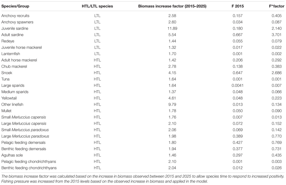
Table 1. Details on the species for which fishing pressure was increased in the various scenarios.
Within the Fishing on Prey scenario, fishing pressure was increased only on selected, fished, low trophic level (LTL) species, namely: anchovy recruits and spawners, sardine recruits and spawners, redeye, juvenile horse mackerel and lanternfish. These species make up about two thirds of the modeled biomass (excluding all plankton and detritus) and half of the modeled catch. These species all showed an increase in biomass under the Increased PP Only scenario making it likely that, under such conditions, fishing pressure on these species could be increased. Within the Fishing on Predators scenario, fishing pressure was increased only on selected high trophic level (HTL) species that increased in biomass under increased PP conditions, namely: adult horse mackerel, chub mackerel, snoek, tuna, large sparids, medium sparids, yellowtail, other linefish, mullet, all hake species, all other demersal species, and pelagic- and benthic-feeding chondrichthyans. These HTL species make up only a fifth of the modeled biomass within the ecosystem (excluding all plankton and detritus), however, account for just under half of the modeled catch. Finally, fishing pressure was increased on all the above mentioned low and HTL species, referred to as the Fishing on Predators and Prey scenario.
The model fitted to 2015 was then run from 2016 to 2040, changing primary productivity of large-celled phytoplankton, and/or fishing mortality rates of selected fished groups, depending on the scenarios examined. In the case of altered fishing, the increased levels of F per species (see Table 1) were applied as simple, constant, higher Fs over the altered fishing simulation period, based on factors of biomass change in baseline versus high productivity biomass levels in 2025 (see explanation above). The biomass and catches varied more in initial simulation years so that where indicator values were examined, results were extracted for the last 10 years of the simulation period (years 2016 to 2040), once the modeled ecosystem and fisheries had stabilized at these new fished and productivity levels.
This approach varies from other indicator studies that tend to increase fishing pressure by the same relative proportions with respect to a baseline (e.g., Fmsy) on all high and LTL species under increased fishing pressure scenarios (e.g., Ortega-Cisneros et al., 2018; Shin et al., 2018). The aim here, however, also differs from those studies. Rather than trying to identify how much an ecosystem can be exploited before it collapses, here we tried to identify sensible increases in removals that would allow increased catches without precipitating a declining state of the ecosystem. Accordingly, the key here was to only remove species that have shown some recovery over the 10 years of increased PP, not those species that showed no trend or a decline, therefore avoiding testing scenarios of overexploitation of vulnerable species.
Assessing Ecosystem Trends Under Each Scenario
The novel decision tree framework described in Lockerbie et al. (2016), and applied in Lockerbie et al. (2017a,b), was adjusted for use in this study. This framework has been used to assess the state and trends in multiple marine ecosystems, assessing the influence of both fishing pressure and the environment on the ecosystem to assess overall state. Indicators used in the framework are derived from the IndiSeas project. However, from the entire suite of IndiSeas indicators (Blanchard et al., 2010; Shin and Shannon, 2010; Shannon et al., 2014; Lockerbie et al., 2016), some indicators were not calculable from the model outputs, such as fish length, while others pertain to the fishing scenario descriptors (intrinsic vulnerability index, marine trophic index, and inverse fishing pressure) which are immaterial in this context wherein we are directly manipulating fishing manually. Therefore, we have focused on ecological, non-fishing strategy indicators within this study. Namely proportion of predators, catch, trophic level of the modeled community (TLmc) and trophic level of landings (TL landings). These indicators still cover a range of desired traits of IndiSeas indicators including maintaining ecosystem structure and functioning, conservation of biodiversity and maintaining ecosystem stability.
As ecological time series are frequently characterized by autocorrelation due to ecosystem dynamics it was necessary to try and account for this when identifying indicator trends. Therefore, a linear model was fitted to each indicator using a generalized least square regression. This involved a two-stage estimation process, following previous IndiSeas procedure (see Coll et al., 2008; Blanchard et al., 2010), to account for autocorrelation in the residuals and to satisfy regression assumptions. Firstly, an ordinary least-squares regression model was used to fit a straight-line model. However, if autocorrelation was detected (defined as a p-value > 0.05 in a Durbin–Watson test) then we proceeded to stage two. Stage two involved the application of a generalized least-square regression to fit the straight-line model, with more flexibility in the assumptions about the error terms (Blanchard et al., 2010), i.e., e (N (0, Σ). Here, Σ is a covariance matrix based on the assumption of e having a temporal dependence structure following an autoregressive process of order 1 [AR(1)] (Coll et al., 2008; Blanchard et al., 2010). The magnitude of the trend was detected based on whether the slope was significantly different from zero (Note: These tests were conducted on standardized indicator values to allow a comparison of trends. Indicators were standardized by subtracting the mean and dividing by the standard deviation).
Adjusting the novel score-based approach developed in Lockerbie et al. (2016), where indicators were categorized based on the significance of trends, here indicator trends were attributed a score based on whether the slope was significantly different from zero and the magnitude of detected trends. The scoring system has been formulated so that higher scores are attributed to a negative trend (i.e., negative effect on ecosystem based on the formulation of IndiSeas indicators), and therefore higher overall scores are attributed to adversely impacted ecosystems. In the analysis of indicator trends a significance level of 0.1 is used, accounting for high interannual variability within time series (Howard et al., 2007). Five scoring categories were used to classify detected trends based on the magnitude of the trend: strong positive trend (slope 0.05 to 0.1) = 1; moderate positive trend (slope 0 to 0.05) = 2; no trend (slope not significantly different from zero) = 3; moderate negative trend (slope 0 to -0.05) = 4; and strong negative trend (slope -0.05 to -0.1) = 5. These categories were selected based on frequency models of both positive and negative trends. Typically, the next step in the application of the framework was to determine the impact of the fishing pressure and environmental variability on indicator trends. However, in contrast to previous studies using this framework, since both the environment and fishing pressure were being manually manipulated in the model the addition of such score adjustments seemed superfluous in this study. Based on these trends in indicators, an overall ecosystem score was calculated and the ecosystem could be placed into one of five categories: improving, possibly improving, no improvement or deterioration, possibly deteriorating or deteriorating (Table 2).
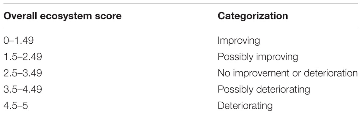
Table 2. Overall ecosystem scores (after application of weightings) and corresponding ecosystem categories of ecosystem classification [adjusted from Lockerbie et al. (2016)].
Catch and TL landings were not included in the decision tree framework as ecological state indicators but were rather used in end-state analyses. However, it is important to consider the fact that the TL landings is likely strongly influenced by the increased fishing pressure being implemented in the model when assessing the influence of the observed trends on the ecosystem. However, as this indicator was also influenced by changes in species for which fishing pressure was not increased in the various scenarios, the decision was made to retain this indicator in this study. Together with the decision-tree based on the three biomass-based indicators, and the end-state analyses based on all five indicators (Table 3), analyses allowed us to better understand and interpret the influence of fishing pressure on the ecosystem under each scenario. In the original applications of this framework [e.g., Lockerbie et al. (2016)] the catch-based indicators would have been included as “fishing pressure indicators.” However, as fishing pressure was already forced in these scenarios, the decision was made not to try include these indicators in decisions trees, to avoid compounding the identified influence of fishing pressure.
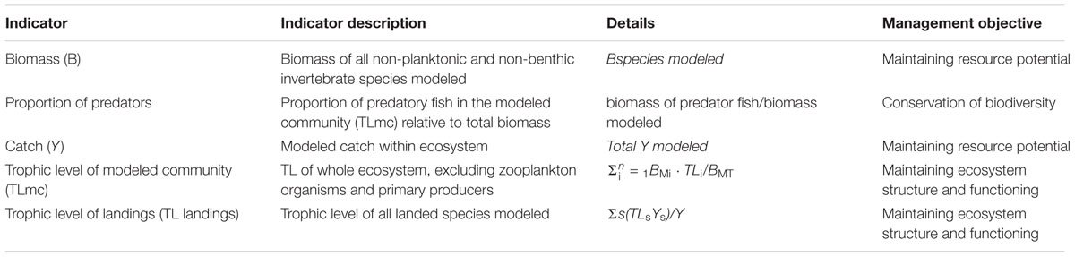
Table 3. Description of indicators used in this study, alongside equations of how indicators were calculated.
For the end-state analysis, an ANOVA was used to compare the means of all six indicators between the five scenarios modeled. Data from the final 10 years of each modeled data series were used, allowing a comparison of the relative future well-being of the ecosystem under each scenario. The significance in the difference between the ANOVAs was determined using a Tukey post hoc test.
It is typical, in simulation studies, to perform sensitivity analyses to assess the implications of assumptions that are made. This would hold true for the current framework, where assumptions are made in terms of both fishery selectivity and the increases in fishing pressure. However, as the purpose of the present study is at this stage is purely to explore the ability of the framework to capture modeled ecosystem changes arising from a simple yet feasible climate scenario, this step has not yet been included. However, it would be a necessary step if this framework were to be used as a tool to inform fisheries managers and stakeholders in a “real world” simulation.
Results
Baseline Scenario
The Baseline Scenario was run as a “status quo” version of the model. In this case current levels of fishing pressure and the current environmental regime were kept at the same level as in the last year to which the model was fitted, namely 2015.
Under this scenario there were no significant trends in either biomass or TLmc, while there was a moderate increase in the proportion of predators. While fishing pressure and PP were not increased in this scenario, the underlying environmental conditions and the maintained fishing pressure would both have somewhat impacted indicator trends. The lack of significant trends in biomass and TLmc likely resulted from the lack of forcing in fishing pressure and environmental drivers, such that the ecosystem muddled along in a similar state to that at the start of the simulation (2015) and, as would be expected, there were therefore no changes in species/groups large enough to be detected in the ecosystem indicators. The overall ecosystem score was calculated as 2.66 and therefore the ecosystem was classified as neither improving nor deteriorating in this scenario (see Table 4). This is in line with what was found in the final period of Lockerbie et al. (2016), from 2004 to 2010, suggesting the framework was able to successfully categorize the modeled ecosystem, and/or that the modeled ecosystem state matched that based on research survey data-derived indicators.
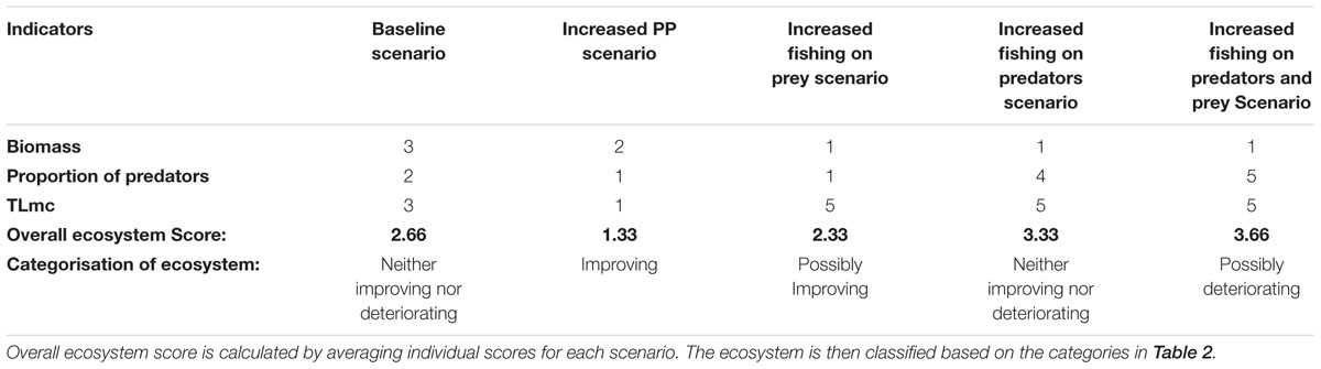
Table 4. Summary of indicator trend scores.
Increased Primary Production Only Scenario
The Increased PP Only scenario was run to provide an easy method of understanding which trends arose from changes in PP and which arose from changes in fishing pressure. When upwelling increases there is, generally, a substantial increase in PP due to increased nutrients. This increase in production will propagate through the food web, with lower trophic level species reacting more quickly to changes in PP, whereas it takes longer for positive effects to reach higher trophic levels. Therefore, it is likely that LTL species will increase first, followed in later years by increases in HTL species.
Strong positive trends were detected in all indicators in this modeled scenario, suggesting that increased upwelling (modeled via increased PP) would have very positive impacts on the ecosystem if there was no increase in fishing pressure. In applying the scoring framework, based on the lack of change in fishing pressure, it can be assumed that the increases observed in all indicators resulted from the increased PP. The ecosystem received an overall score of 1.33, and was therefore classified as improving over this period, again supporting the hypothesized positive influence increased PP would have on the ecosystem (see Table 4).
Increased Fishing on Prey Scenario
Under this model scenario, fishing pressure was increased on selected LTL species (see Table 1) in conjunction with increased PP. LTL species generally react faster to changes in environmental conditions and their populations can expand rapidly under ideal conditions (Cury et al., 2000), such as increased PP resulting from increased upwelling. It is, therefore, unsurprising that several LTL species such as anchovy, sardine, and redeye showed strong increases in biomass in the 10 years over which PP increased (see Supplementary Figure S3). Strong positive trends were observed in biomass and the proportion of predators were observed, suggesting that even under increased fishing pressure there were positive impacts on the ecosystem. The increase in biomass can be linked to increased PP under increased upwelling conditions, which propagates through the food web resulting in increases in both low and HTL species. The increase in the proportion of predators likely resulted from both an increase in biomass of HTL species (supported by an increased forage base under increased PP) and the continued increase in LTL species even under increased fishing pressure (see Supplementary Figure S3).
There was also a strong negative trend observed in the TLmc. It can be assumed that this trend resulted from the increase in biomass of forage species (including those not fished) under the increased PP conditions, rather than from a decline in predatory biomass, based on the increase in the proportion of predators that has also been observed.
The ecosystem received an overall score of 2.3 and was therefore classified as possibly improving under this scenario (see Table 4).
Increased Fishing on Predators Scenario
Under the Fishing on Predators model scenario, fishing pressure was increased on selected HTL species (see section “Materials and Methods”) in conjunction with increasing PP. In this scenario there was a strong positive trend in biomass, suggesting that even when fishing pressure is increased there is still a significant increase in fish community biomass under increased PP conditions. There was, however, a moderate negative trend in the proportion of predators. This contrasts to the Increased PP Only and Fishing on Prey scenarios where the proportion of predators showed strong positive trends. It is likely that the increased fishing pressure on only selected HTL species has resulted this declining trend, however, as fishing pressure was not increased on all HTL species there has not been an overexploitation to the point where the proportion of predators in the ecosystem has begun to strongly decline.
A strong negative trend in the TLmc was observed in this scenario. This decline in trophic level can be linked both the declining proportion of predators as well as to increases in LTL species, such as anchovy and lanternfish under reduced predation pressure (see Supplementary Figures S4a,b). To expand, fishing pressure on LTL species has not been increased in this scenario and therefore fishing pressure on higher trophic level species may have released some smaller species from predation pressure, allowing a proliferation of these species and helping to explain the decline of TLmc.
The ecosystem received a score of 3.33 and was therefore categorized as neither improving nor deteriorating in this scenario (see Table 4).
Increased Fishing on Predators and Prey Scenario
This model scenario yielded the most negative changes within the ecosystem. While biomass showed a strong positive trend, similarly, to the previous scenarios, there strong negative trends in the proportion of predators and in TLmc. The increase in biomass can be linked to the increase in PP in this scenario and is unlikely to be related to the increase in fishing pressure. The increased fishing pressure on both HTL and LTL species clearly has negative impacts on predatory fish species, resulting in a decline in some HTL species, particularly benthic and pelagic-feeding demersal species. Under this scenario, there is maintenance of high biomass of LTL species such as anchovy, redeye, lanternfish, and lightfish when predatory fish are removed from the ecosystem (see Supplementary Figure S5). It is therefore likely that an increase in LTL species could have contributed to the decline in both the proportion of predators and TLmc.
The ecosystem received a score of 3.66 and was therefore categorized as possibly deteriorating (see Table 4).
Relative End-State of the Ecosystem
To assess the relative end-state of the ecosystem under each scenario, an ANOVA was conducted using the final 10 years of the model output for each scenario, allowing us to visualize and compare the difference in the end-state of indicators (Figures 1A–E). ANOVAs were compared the mean of the last 10 years of indicator values (calculated from the model output) in order to compare the end-state of the ecosystem under each scenario. This was followed by a Tukey post hoc test to identify whether the observed differences in indicators between the scenarios were statistically significant.
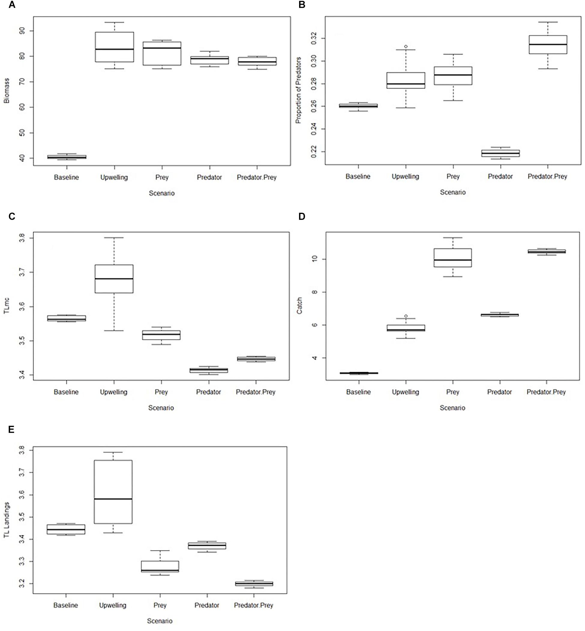
Figure 1. (A–E) Boxplots of ANOVA results for each indicator comparing the end-state (final 10 years of data) for each scenario. (A) Biomass, (B) Proportion of predators, (C) Trophic level of the modeled community (TLmc), (D) Catch, and (E) Trophic level of landings.
In terms of biomass (Figure 1A), significantly lower values were observed in the Baseline scenario compared to all other scenarios (Tukey’s, p < 0.05). This was not surprising as biomass in all scenarios, except for the baseline scenario, showed a significant increase over the simulation period. Biomass was highest in the Increased PP Only and Fishing on Prey Scenarios, and not significantly lower in the Fishing on Predators and Fishing on Predators and Prey scenarios. This suggests that there would be a strongly positive influence of increased PP on fish biomass, even when fishing pressure is increased. This significant increase in biomass under all fishing scenarios is a good sign for fisheries managers, as it suggests that there may be scope to increase fishing pressure while still maintaining relatively healthy biomass levels within the ecosystem. However, based on trends in other indicators, attention would need to be given as to what species can be further exploited and by how much, to ensure the ecosystem does not collapse.
A range of values for the portion of predators were observed across the various scenarios (Figure 1B). Values for this indicator were significantly lower in the Fishing on Predators scenario than in all other scenarios (Tukey’s, p < 0.05), including the Baseline scenario. This suggests that, despite increased overall system biomass in the Fishing on Predators scenario, increased exploitation of predatory species could negatively impact the ecosystem. However, interestingly, the Fishing on Predators and Prey scenario had a significantly higher proportion of predators compared to all other scenarios (Tukey’s, p < 0.05). This suggests that predators in the ecosystem fared better when a range of trophic levels are fished, compared to targeting only HTL species. Yet the declining trends in the proportion of predators in this scenario should provoke caution as to whether such fishing pressure would be sustainable in the long term. However, in the Fishing on Predators scenario it appears that the low proportion of predators is linked to increases in LTL species, given the alleviation of some predation pressure in the system (see Supplementary Figure S4). The Prey scenario showed a relatively high proportion of predators, significantly higher than in the Baseline, Increased PP and Fishing on Predators scenarios (Tukey’s, p < 0.05). This implied that, even when fishing pressure was increased on LTL species, these species were not negatively impacted to a point where there would be a detrimental effect on higher trophic levels feeding on the fished forage species. Based solely on this indicator, there may therefore be even further potential to increase fishing pressure on these LTL species if PP, linked to predicted increased in upwelling, was to increase in future. However, the full suite of indicators needs consideration.
The TLmc was significantly higher in the Increased PP Only scenario (Tukey’s, p < 0.05), with the three fishing scenarios showing significantly lower levels than both the Increased PP and Baseline scenarios (Figure 1C). This was not surprising as in all fishing scenarios there was a significant decreasing trend observed in TLmc (Table 4). The lowest TLmc values were observed in the Fishing on Predators scenario. As observed in the proportion of predators, this was likely due to a combination of increased removal of larger species as well as an increase in smaller species when predation pressure is relaxed. However, in contrast to the proportion of predators, the Fishing on Predators and Prey scenario showed very low TLmc values and was not significantly different to the values in the Fishing on Predators scenario (Tukey’s, p > 0.05). This suggests that increasing fishing pressure on all levels, while better for predatory fish (as observed from the high proportion of predators in this scenario) may not result in an improved ecosystem state, which would be desired to ensure food security for future generations. This is also highlighted by the declining trends observed in both TLmc and the proportion of predators under the Increased Fishing on Predators and Increased Fishing on Predators and Prey scenarios, despite the high levels of predators. As an increase biomass of LTL level species was observed even when fishing pressure is increased on selected species (see Supplementary Material), it is possible that the low TLmc values in all fishing scenarios could be linked to increased biomass of LTL species under the increased PP conditions.
Catch within the ecosystem showed a wide range of values throughout the various scenarios (Figure 1D), with all scenarios in which modeled PP is increased showing significantly higher catch than the Baseline scenario. The low catch values observed in the Baseline scenario reflect the lower system biomass observed in that scenario. The catches observed in the Fishing on Prey and Fishing on Predators and Prey scenarios were significantly higher than the other scenarios (Tukey’s, p < 0.05). However, declining trends in TLmc, TL landings and proportion of predators indicators in the Fishing on Predators and Prey scenario suggest that care should be taken under this scenario, as declining trends are a warning sign of ecosystem degradation (i.e., loss of biological function/productivity).
As previously mentioned, catch and TL landings were not included in the decision trees but can be useful in understanding the effects of fishing pressure on the ecosystem. Similarly, to TLmc, the highest TL landings values were observed in the Increased PP scenario, with all fishing pressure scenarios showing lower trophic levels than both the Baseline and Increased PP scenarios (Figure 1E). Out of the fishing pressure scenarios, TL landings was highest in the Fishing on Predators scenario. This is not surprising as fishing pressure on HTL species was increased in this scenario. However, interestingly, the TL landings values were lower in the Fishing on Predators and Prey scenario compared to the Prey scenario. It would be expected that when fishing pressure was increased only on LTL species, the trophic level of the landings would be lowest, rather than in a scenario where fishing pressure on both HTL and LTL species were increased. However, it should be remembered that fishing pressure was not uniformly increased across all fished groups, but instead depended on the observed model increase in abundance of the fished groups under increased PP. Thus, given the greater relative increases in abundance of LTL species under increased PP, modeled relative fishing pressure was increased more for these groups than for higher TL groups.
Discussion
Fishing Strategies Under Enhanced Primary Production Conditions
Our understanding of the future of marine ecosystems needs to improve if we are to adapt to the unprecedented levels of change that have been predicted to occur in future decades. However, as change at this level has not yet been experienced, it is hard to determine what might lie in the futures of ecosystems. Using scenarios that cover a range of possible outcomes should give marine scientists, fisheries managers and stakeholders a better idea of possible outlooks. Knowledge of potential futures could allow some preparation for conceivable changes and possibly provide early warning signs of detrimental changes occurring within ecosystems, allowing some mitigation for these effects. Understanding the cause of observed trends in indicators was made much simpler through the use of model simulations, where both the environment and fishing pressure have been forced by predetermined amounts. However, the way in which this (and any other ecosystem model) is forced does not allow us to capture complete ecosystem dynamics, and therefore may not be as all-encompassing as would be needed for us to fully understand and react to changes in ecosystem dynamics.
This study aimed to explore potential future states of the Southern Benguela ecosystem under increased PP conditions and with various scenarios of increased fishing pressure. It emerged that an increase in PP could have positive effects on the Southern Benguela ecosystem as a whole. Increased PP, which could result from increased upwelling, resulted in an increase in biomass that propagated throughout the ecosystem, impacting both high and LTL species. This was clearly evident in the Increased PP Only scenario where all indicators in the decision tree analysis showed positive trends (Table 4). Travers-Trolet et al. (2014) observed that changes in the ecosystem caused by an increase in upwelling-favorable wind stress propagate through the food web, causing increases in phytoplankton, zooplankton, forage fish, and top predators when the ecosystem is under no or moderate exploitation. Similar results were observed in this study, with the ecosystem showing more positive results when fishing pressure was lowest, or when it was exerted on more resilient LTL species.
However, it is important to note that many studies have shown that, in general, indicators are more specific to fishing pressure than to environmental variability, although that is dependent on the ecosystems being considered (Ortega-Cisneros et al., 2018; Shin et al., 2018). Therefore, we should consider that the trends observed in this study may be more likely to result from increased fishing pressure than from increased PP. The higher specificity of IndiSeas indicators to fishing pressure than to environmental changes (Shin et al., 2018; where specificity is the extent to which an indicator responds to fishing as opposed to other drivers), could help explain the numerous negative indicator trends observed in this study under the increased fishing pressure scenarios even when we have increased productivity in the ecosystem. However, alongside this, the constant fishing mortalities applied into the future (during and after the 10 years of increasing primary productivity), as well as the expected time lags between increased PP and modeled responses in fish biomass, provide additional explanations for some of the negative indicator trends observed.
The influence of increased production alongside increased fishing pressure on ecosystems has been evaluated in several other studies using multiple other models (e.g., Travers-Trolet et al., 2014; Fu et al., 2018; Shin et al., 2018). These studies have observed that, in some cases, a decrease in fishing pressure is not sufficient to cause a change in indicator trend if environmental variability changes simultaneously. Therefore, if the modeled increases in fishing pressure were implemented it would be vital to closely monitor environmental change to reduce the risk of ecosystem collapse. Results of these studies also suggest that under increased environmental variability, it is possible that indicators will become less specific to fishing pressure (Shin et al., 2018).
It appears that the more rapid response times of lower trophic level species, such as small pelagic fish, to such changes in environmental conditions would potentially result in significant increases in their biomass if higher total cumulative upwelling, and hence higher levels of PP, became the “new normal.” These positive effects of increased PP on ecosystem indicators are an encouraging sign for fisheries managers and stakeholders, who may be able to further exploit the ecosystem in future in a sustainable way, helping to safeguard food security in years to come. However, both decision trees and end-state analyses suggest that any increases in fishing pressure would need to be carefully considered and monitored to avoid ecosystem degradation.
Results from the three fishing scenarios discussed above suggest that under increased PP conditions it may be possible to increase fishing pressure on certain species and still maintain, or even improve, ecosystem state. For example, even when fishing pressure was increased on LTL species in the Fishing on Prey scenario, the ecosystem was still classified as possibly improving (Table 4). By comparison, the end-state analysis revealed that in the Fishing on Predators scenario the proportion of predators, TLmc and TL Landings are all significantly lower than the baseline scenario (Figures 1B,C,E), which, together with the classification as “neither improving nor deteriorating” in the decision tree, highlights the potentially detrimental effects of increased fishing pressure on HTL species. These results suggest that care will need to be taken when selecting which species can be more heavily exploited under climate change, and by how much, as it is best to avoid reaching a point where indicators show declining trends to prevent ecosystem degradation.
This is further evidenced by the contrast between the outcomes of the decision trees and that of the end-state analyses in the case of the Fishing on Predators and Prey scenario. The decision tree analysis suggests that the ecosystem would possibly be deteriorating under the Fishing on Predators and Prey scenario, due to the declining trends observed in indicators. In contrast, the end-state analysis shows that the proportion of predators and catch are highest in this scenario, while biomass also remained high (Figures 1A,B,D). These results may support balanced harvesting, which suggests that ecosystems will fare better when fishing pressure is distributed more evenly across the ecosystem, rather than implementing selective fishing pressure on certain target species (e.g., Garcia et al., 2012, 2015). Yet, despite these high indicator values, the negative trends observed in TLmc and the proportion of predators suggest that if this level of fishing pressure was to continue further into the future, the ecosystem end-states may in fact deteriorate. A future solution may therefore lie in a modification to the Prey scenario. When fishing pressure was increased on selected LTL species, the predators in the ecosystem showed some recovery (e.g., the increase in the proportion of predators in Table 4). Therefore, the best way forward may be to delay implementing balanced harvesting until the ecosystem has been allowed time to recover from the previous impacts of fishing pressure, in order to avoid declining indicator trends.
In summary, the decision tree analyses of the Fishing on Predators and Prey and Fishing on Predators scenarios suggest caution must be taken when deciding how to increase fishing pressure under climate change.
Catch Considerations
One of the most important indicators to look at in terms of end-state of the ecosystem is the total catch within the ecosystem. While catch is not included as an indicator within the decision trees, it is used in the calculation of other indicators in this study, such as TL Landings (see Table 3) and is possibly the indicators of most interest to fisheries managers and stakeholders. From Figure 1D it is clear that under increased PP conditions, the catch within the ecosystem increased, with highest catch being observed in the Fishing on Prey and Fishing on Predators and Prey Scenario (both of which produced roughly three times the levels of catch). These increases in catch would be of most significance to fisheries managers and stakeholders as this suggests that, under the plausible conditions of increased PP if upwelling were to increase, it may be possible to expand certain fisheries. However, due to the declining trends observed in some ecological indicators, the Fishing on Predators and Prey scenario may not necessarily be a sustainable option going forward.
Therefore, based on the results of this study, the future of the ecosystem appears most positive under the Fishing on Prey scenario. This scenario allowed increased fishing pressure on a range of important LTL species, allowing an expansion of fisheries, while still allowing the ecosystem to be classified as possibly improving. Under this scenario there may even be potential scope for further increases of fishing pressure on these species, and even possibly some HTL species, if carefully monitored to avoid over exploitation. However, this study would also benefit from further analysis on the effect of the potential increases and decreases in biomasses of multiple commercially important species under the various scenarios on the human component of the ecosystem, as reiterated in the next section.
Future Research Considerations
Despite the apparent success of this study, it is important to note several factors that have not been considered. For example, the increase in PP used in this study has been oversimplified. The impacts of other factors, such as extreme weather events, changes in ocean stratification (Rykaczewski and Dunne, 2010) and changes is energy of oceanic vortices (Gruber et al., 2011), have not been accounted for. It is therefore possible that the increase we have suggested could have been either over- or underestimated. However, as the increase in PP used here falls within a range that has already been observed within the Southern Benguela (see Lamont et al., 2018), certainly it can be considered a plausible scenario for the future of the ecosystem.
There are, however, several other factors associated with an increase in upwelling that have not been considered, and which may somewhat dampen the positive effects associated with the observed (modeled) increased production. Within the Southern Benguela, increased upwelling could cause regional cooling, due to increased cold water being advected to the surface, as has been observed in Peruvian upwelling ecosystem (Gutiérrez et al., 2011). Some eggs and larvae have limited temperature ranges (e.g., King et al., 1978) and would not survive prolonged periods in such temperatures, resulting in some species being negatively impacted by increased upwelling. Another factor that has not been considered in this study is the physical impact that increased wind would have on some eggs, larvae and smaller prey species. Increased turbulence and offshore transport resulting from increase wind can result in excessive the transport of larvae and prey species away from the important nursery grounds within the Southern Benguela (Shannon et al., 1996; Shannon, 1998). It is possible that increased upwelling could also result in deeper wind-driven mixing and increased light limitation, resulting in a reduction of phytoplankton production. Ideally all these factors should be considered and included where possible in future modeling of potential climate scenarios. Until such factors can be included in the model, it is necessary to refer to the environmental scenario described in this study as an increased PP scenario, rather than a true increased upwelling scenario.
Yet, for the purpose of this exploratory study, it was more crucial to see if the framework of indicators and decision trees was able to capture the dynamics of the ecosystem under the selected scenarios and give meaningful results. Following the success of this framework in categorizing the ecosystem, a wider range of potential environmental changes within the ecosystem could be modeled and included to give a better understanding of the future of this ecosystem, informing fisheries managers and stakeholder and allowing a better chance of protecting the future of the Southern Benguela. Such scenarios, and the associated planning, could prove invaluable in safeguarding the future of the Southern Benguela and its resources. However, we acknowledge the fact that the true success of such a framework lies in its successful communication to stakeholders and managers. Therefore, the next step in the application of such a framework should be its discussion with the appropriate audiences. For example, fisheries managers may find it helpful for sensitivity tests to be run on the three fishing scenarios so far presented, and for cross-fleet constraints to be addressed; the current model framework assumed that species were largely caught independently of one another. In addition, extending this study to explore economic and social values of potential catches under the different scenarios would be a desirable next step in the light of recognizing the importance of human well-being indicators in an EAF.
Data Availability
The datasets generated for this study are available on request to the corresponding author.
Author Contributions
EL and LS conceived the manuscript. LS ran the model. EL synthesized the model outputs into the relevant indicators and conducted data analysis. EL led the writing with substantial contributions from LS.
Funding
This work was supported wholly by the South African Network for Coastal and Oceanic Research through the National Research Foundation of South Africa (Grant Number 112682). This work was partly funded by the SARCHI Chair in Marine Ecology and Fisheries, through co-supervision by LS.
Conflict of Interest Statement
The authors declare that the research was conducted in the absence of any commercial or financial relationships that could be construed as a potential conflict of interest.
Acknowledgments
We would like to acknowledge the South African Scientific Research Chair Initiative, of the Department of Science and Technology and administered by the National Research Foundation (NRF), through the chair in Marine Ecology and Fisheries.
Supplementary Material
The Supplementary Material for this article can be found online at: https://www.frontiersin.org/articles/10.3389/fmars.2019.00380/full#supplementary-material
References
Bakun, A. (1990). Global climate change and intensification of coastal ocean upwelling. Science 247, 198–201. doi: 10.1126/science.247.4939.198
Bakun, A., Black, B. A., Bograd, S. J., Garcia-Reyes, M., Miller, A. J., Rykaczewski, R. R., et al. (2015). Anticipated effects of climate change on coastal upwelling ecosystems. Curr. Clim. Change Rep. 1, 85–93. doi: 10.1007/s40641-015-0008-4
Blanchard, J. L., Coll, M., Trenkel, V. M., Vergnon, R., Yemane, D., Jouffre, D., et al. (2010). Trend analysis of indicators: a comparison of recent changes in the status of marine ecosystems around the world. ICES J. Mar. Sci. 67, 732–744. doi: 10.1093/icesjms/fsp282
Bland, L. M., Rowland, J. A., Regan, T. J., Keith, D. A., Murray, N. J., Lester, R. E., et al. (2018). Developing a standardized definition of ecosystem collapse for risk assessment. Front. Ecol. Environ. 16:29–36. doi: 10.1002/fee.1747
Brown, P., Painting, S., and Cochrane, K. (1991). Estimates of phytoplankton and bacterial biomass and production in the northern and southern Benguela ecosystems. S. Afr. J. Mar. Sci. 11, 537–564. doi: 10.2989/025776191784287673
Bundy, A., Shannon, L. J., Rochet, M. J., Neira, S., Shin, Y. J., Hill, L., et al. (2010). The good(ish), the bad, and the ugly: a tripartite classification of ecosystem trends. ICES J. Mar. Sci. 67, 745–768. doi: 10.1093/icesjms/fsp283
Cheung, W. W., Lam, V. W., Sarmiento, J. L., Kearney, K., Watson, R., and Pauly, D. (2009). Projecting global marine biodiversity impacts under climate change scenarios. Fish Fish. 10, 235–251. doi: 10.1111/j.1467-2979.2008.00315.x
Coll, M., Palomera, I., Tudela, S., and Dowd, M. (2008). Food-web dynamics in the South Catalan Sea ecosystem (NW Mediterranean) for 1978–2003. Ecol. Modell. 217, 95–116. doi: 10.1016/j.ecolmodel.2008.06.013
Coll, M., Shannon, L., Kleisner, K., Juan-Jordá, M., Bundy, A., Akoglu, A., et al. (2016). Ecological indicators to capture the effects of fishing on biodiversity and conservation status of marine ecosystems. Ecol. Indic. 60, 947–962. doi: 10.1016/j.ecolind.2015.08.048
Cropper, T. E., Hanna, E., and Bigg, G. R. (2014). Spatial and temporal seasonal trends in coastal upwelling off Northwest Africa, 1981–2012. Deep Sea Res. Part 1 Oceanog. Res. Papers 86, 94–111. doi: 10.1016/j.dsr.2014.01.007
Crowder, L. B., Hazen, E. L., Avissar, N., Bjorkland, R., Latanich, C., and Ogburn, M. B. (2008). ). The impacts of fisheries on marine ecosystems and the transition to ecosystem-based management. Annu. Rev. Ecol. Evol. Syst. 39, 259–278. doi: 10.1146/annurev.ecolsys.39.110707.173406
Cury, P., Bakun, A., Crawford, R. J., Jarre, A., Quinones, R. A., Shannon, L. J., et al. (2000). ). Small pelagics in upwelling systems: patterns of interaction and structural changes in “wasp-waist” ecosystems. ICES J. Mar. Sci. 57, 603–618. doi: 10.1006/jmsc.2000.0712
de Moor, C. L. (2016). Assessment of the South African Anchovy Resource Using Data from 1984-2015: results at the Posterior Mode. DAFF Branch Fisheries Document. FISHERIES/2016/OCT/SWG-PEL/ 46, 41.
Finkel, Z. V., Beardall, J., Flynn, K. J., Quigg, A., Rees, T. A. V., and Raven, J. A. (2009). Phytoplankton in a changing world: cell size and elemental stoichiometry. J. Plankton Res. 32, 119–137. doi: 10.1093/plankt/fbp098
Fu, C., Travers-Trolet, M., Velez, L., Grüss, A., Bundy, A., Shannon, L. J., et al. (2018). Risky business: the combined effects of fishing and changes in primary productivity on fish communities. Ecol. Modell. 368, 265–276. doi: 10.1016/j.ecolmodel.2017.12.003
Garcia, S., Kolding, J., Rice, J., Rochet, M.-J., Zhou, S., Arimoto, T., et al. (2012). Reconsidering the consequences of selective fisheries. Science 335, 1045–1047. doi: 10.1126/science.1214594
Garcia, S., Rice, J., and Charles, A. (2015). Balanced harvesting in fisheries: a preliminary analysis of management implications. ICES J. Mar. Sci. 73, 1668–1678. doi: 10.1093/icesjms/fsv156
Gruber, N., Lachkar, Z., Frenzel, H., Marchesiello, P., Münnich, M., McWilliams, J. C., et al. (2011). Eddy-induced reduction of biological production in eastern boundary upwelling systems. Nat. Geosci. 4:787. doi: 10.1038/NGEO1273
Gutiérrez, D., Bouloubassi, I., Sifeddine, A., Purca, S., Goubanova, K., Graco, M., et al. (2011). Coastal cooling and increased productivity in the main upwelling zone off Peru since the mid-twentieth century. Geophys. Res. Lett. 38:L07603 doi: 10.1029/2010GL046324
Harley, C. D., Randall Hughes, A., Hultgren, K. M., Miner, B. G., Sorte, C. J., Thornber, C. S., et al. (2006). The impacts of climate change in coastal marine systems. Ecol. Lett. 9, 228–241. doi: 10.1111/j.1461-0248.2005.00871.x
Howard, J. A., Jarre, A., Clark, A., and Moloney, C. (2007). Application of the sequential t-test algorithm for analysing regime shifts to the southern Benguela ecosystem. Afr. J. Mar. Sci. 29, 437–451. doi: 10.2989/AJMS.2007.29.3.11.341
Jackson, J. B., Kirby, M. X., Berger, W. H., Bjorndal, K. A., Botsford, L. W., Bourque, B. J., et al. (2001). Historical overfishing and the recent collapse of coastal ecosystems. Science 293, 629–637. doi: 10.1126/science.1059199
Jones, M. C., Dye, S. R., Pinnegar, J. K., Warren, R., and Cheung, W. W. (2015). Using scenarios to project the changing profitability of fisheries under climate change. Fish Fish. 16, 603–622. doi: 10.1111/faf.12081
King, D., Robertson, A., and Shelton, P. (1978). Laboratory observations on the early development of the anchovy Engraulis capensis from the Cape Peninsula. Fish. Bull. S. Afr. 10, 37–45.
Lamont, T., Barlow, R., and Kyewalyanga, M. (2014). Physical drivers of phytoplankton production in the southern Benguela upwelling system. Deep Sea Res. Part 1 Oceanogr. Res. Papers 90, 1–16. doi: 10.1016/j.dsr.2014.03.003
Lamont, T., García-Reyes, M., Bograd, S., van der Lingen, C., and Sydeman, W. (2018). Upwelling indices for comparative ecosystem studies: variability in the Benguela upwelling system. J. Mar. Syst. 188, 3–16. doi: 10.1016/j.jmarsys.2017.05.007
Lockerbie, E. M., Coll, M., Shannon, L. J., and Jarre, A. (2017a). The use of indicators for decision support in Northwestern mediterranean sea fisheries. J. Mar. Syst. 174, 64–77. doi: 10.1016/j.jmarsys.2017.04.003
Lockerbie, E. M., Lynam, C. P., Shannon, L., and Jarre, A. (2017b). Applying a decision tree framework in support of an ecosystem approach to fisheries: IndiSeas indicators in the North Sea. ICES J. Mar. Sci. 75, 1009–1020. doi: 10.1093/icesjms/fsx215
Lockerbie, E., Shannon, L., and Jarre, A. (2016). The use of ecological, fishing and environmental indicators in support of decision making in southern Benguela fisheries. Ecol. Indic. 69, 473–487. doi: 10.1016/j.ecolind.2016.04.035
Molinos, J. G., Halpern, B. S., Schoeman, D. S., Brown, C. J., Kiessling, W., Moore, P. J., et al. (2016). Climate velocity and the future global redistribution of marine biodiversity. Nat. Clim. Change 6:83. doi: 10.1038/NCLIMATE2769
Ortega-Cisneros, K., Shannon, L., Cochrane, K., Fulton, E. A., and Shin, Y. J. (2018). Evaluating the specificity of ecosystem indicators to fishing in a changing environment: a model comparison study for the southern Benguela ecosystem. Ecol. Indic. 95, 85–98. doi: 10.1016/j.ecolind.2018.07.021
Pereira, H. M., Leadley, P. W., Proença, V., Alkemade, R., Scharlemann, J. P., Fernandez-Manjarrés, J. F., et al. (2010). Scenarios for global biodiversity in the 21st century. Science 330, 1496–1501. doi: 10.1126/science.1196624
Planque, B. (2015). Projecting the future state of marine ecosystems,“la grande illusion”? ICES J. Mar. Sci. 73, 204–208. doi: 10.1093/icesjms/fsv155
Probyn, T. (1992). The inorganic nitrogen nutrition of phytoplankton in the southern Benguela: new production, phytoplankton size and implications for pelagic foodwebs. S. Afr. J. Mar. Sci. 12, 411–420. doi: 10.2989/02577619209504715
Rademeyer, R., and Butterworth, D. (2016). An initial update of the reference case assessment and related projections for the South African hake resource. DAFF Branch Fisheries document. FISHERIES/2016/MAY/SWG-DEM/ 11, 40.
Roessig, J. M., Woodley, C. M., Cech, J. J., and Hansen, L. J. (2004). Effects of global climate change on marine and estuarine fishes and fisheries. Rev. Fish Biol. Fish. 14, 251–275. doi: 10.1007/s11160-004-6749-0
Roy, C., Weeks, S. J., Rouault, M., Nelson, C. S., Barlow, R. G., and van Der Lingen, C. D. (2001). Extreme oceanographic events recorded in the Southern Benguela during the 1999–2000 summer season. S. Afr. J. Mar. Sci. 97, 465–471.
Rykaczewski, R. R., and Dunne, J. P. (2010). Enhanced nutrient supply to the California Current Ecosystem with global warming and increased stratification in an earth system model. Geophys. Res. Lett. 37:L21606 doi: 10.1029/2010GL045019
Shannon, L. (1998). Modelling environmental effects on the early life history of the South African anchovy and sardine: a comparative approach. Afr. J. Mar. Sci. 19, 291–304. doi: 10.2989/025776198784126638
Shannon, L., Christensen, V., and Walters, C. (2004). Modelling stock dynamics in the southern Benguela ecosystem for the period 1978–2002. Afr. J. Mar. Sci. 26, 179–196. doi: 10.2989/18142320409504056
Shannon, L., Coll, M., Bundy, A., Gascuel, D., Heymans, J. J., Kleisner, K., et al. (2014). Trophic level-based indicators to track fishing impacts across marine ecosystems. Mar. Ecol. Prog. Ser. 512, 115–140. doi: 10.3354/mes10821
Shannon, L., Neira, S., and Taylor, M. (2008). Comparing internal and external drivers in the southern Benguela and the southern and northern Humboldt upwelling ecosystems. Afr. J. Mar. Sci. 30, 63–84. doi: 10.2989/ajms.2008.30.1.7.457
Shannon, L. J., Nelson, G., Crawford, R. J., and Boyd, A. J. (1996). Possible impacts of environmental change on pelagic fish recruitment: modelling anchovy transport by advective processes in the southern Benguela. Glob. Change Biol. 2, 407–420. doi: 10.1111/j.1365-2486.1996.tb00091.x
Shin, Y. J., Houle, J. E., Akoglu, E., Blanchard, J. L., Bundy, A., Coll, M., et al. (2018). The specificity of marine ecological indicators to fishing in the face of environmental change: a multi-model evaluation. Ecol. Indic. 89, 317–326. doi: 10.1016/j.ecolind.2018.01.010
Shin, Y. J., and Shannon, L. J. (2010). Using indicators for evaluating, comparing, and communicating the ecological status of exploited marine ecosystems. 1. The IndiSeas project. ICES J. Mar. Sci. 67, 686–691. doi: 10.1093/icesjms/fsp273
Smith, A. D., Brown, C. J., Bulman, C. M., Fulton, E. A., Johnson, P., Kaplan, I. C., et al. (2011). Impacts of fishing low–trophic level species on marine ecosystems. Science 333, 1147–1150. doi: 10.1126/science.1209395
Sweeney, E. N., McGillicuddy, D. J. Jr., and Buesseler, K. O. (2003). Biogeochemical impacts due to mesoscale eddy activity in the Sargasso Sea as measured at the Bermuda Atlantic Time-series Study (BATS). Deep Sea Res. Part 2 Topic. Stud. Oceanogr. 50, 3017–3039. doi: 10.1016/j.dsr2.2003.07.008
Sydeman, W., García-Reyes, M., Schoeman, D., Rykaczewski, R., Thompson, S., Black, B., et al. (2014). Climate change and wind intensification in coastal upwelling ecosystems. Science 345, 77–80. doi: 10.1126/science.1251635
Travers-Trolet, M., Shin, Y.-J., Shannon, L. J., Moloney, C. L., and Field, J. G. (2014). Combined fishing and climate forcing in the southern Benguela upwelling ecosystem: an end-to-end modelling approach reveals dampened effects. PLoS One 9:e94286. doi: 10.1371/journal.pone.0094286
Walters, C., Christensen, V., and Pauly, D. (1997). Structuring dynamic models of exploited ecosystems from trophic mass-balance assessments. Rev. Fish Biol. Fish. 7, 139–172.
Keywords: scenarios, fisheries management, decision trees, ecosystem-based management, ecosystem wellbeing
Citation: Lockerbie EM and Shannon L (2019) Toward Exploring Possible Future States of the Southern Benguela. Front. Mar. Sci. 6:380. doi: 10.3389/fmars.2019.00380
Received: 25 March 2019; Accepted: 18 June 2019;
Published: 11 July 2019.
Edited by:
Michael Arthur St. John, Technical University of Denmark, DenmarkReviewed by:
M. Robin Anderson, Fisheries and Oceans Canada, CanadaSarah Gaichas, National Oceanic and Atmospheric Administration (NOAA), United States
Geret Sean DePiper, National Oceanic and Atmospheric Administration (NOAA), United States
Copyright © 2019 Lockerbie and Shannon. This is an open-access article distributed under the terms of the Creative Commons Attribution License (CC BY). The use, distribution or reproduction in other forums is permitted, provided the original author(s) and the copyright owner(s) are credited and that the original publication in this journal is cited, in accordance with accepted academic practice. No use, distribution or reproduction is permitted which does not comply with these terms.
*Correspondence: Emma M. Lockerbie, ZW1tYWxvY2tlcmJpZUBnbWFpbC5jb20=