Nutrient Retention in the Swedish Coastal Zone

In this study, the average nutrient filter efficiency of the entire Swedish coastline is estimated to be about 54 and 70% for nitrogen and phosphorus, respectively. Hence, significantly less than half of the nutrient input from land (defined as river discharge and point sources) can be assumed to be exported from coastal waters to the open sea. However, some coastal areas retained more than 100% of the land load and thus, also filter the open Baltic Sea water. These areas with effective filtering of nutrients have low land load per unit coastal area. The filter efficiency was calculated from a 30-years model simulation (1985–2014) of water exchanges and nutrient cycling within the Swedish coastal zone. The average model skill was evaluated to be good or acceptable compared to observations. In addition to the entire Swedish coast, the retention of total nutrient loads in seven larger coastal sub-regions and selected key sites representing different coastal types was also estimated. The modeled long term nutrient retention was found to be associated with the physical characteristics of a water body, such as the surface area, but also the mean depth and residence time of water. In addition, high retention efficiency is associated with high ratio of sediment nutrient content to pelagic nutrient concentrations. On interannual timescales temporal changes in the coastal nutrient pool can have a large influence on perceived nutrient retention. At one site, the phosphorus filter efficiency was actually negative, i.e., the coastal zone transported more phosphorus to the open Baltic Sea than it received from land. The nutrient removal is most efficient close to land, where the area specific retention efficiency is the highest. The variability of both the filter and retention efficiency between coastal regions was found to be large, with a range of approximately 4–1,200% and 0.1–8.5%, respectively.

Introduction

Most of the Swedish coast boarders the brackish, semi-enclosed Baltic Sea while the Swedish West Coast is connected to the Kattegat and Skagerrak system that acts as a transitional zone between the North Sea and the Baltic Sea. The Baltic Sea is shallow with a mean water depth of 54 m [Gotland Deep and Landsort Deep are about 250 and 459 m, respectively; see Seifert and Kayser (1995)]. It is characterized by large vertical and horizontal salinity gradients (e.g., Leppäranta and Myrberg, 2009) from the entrance up to the Bothnian Bay. The Baltic Sea is connected to the Kattegat through the Danish straits of Öresund, the Great Belt, and the Little Belt where the entrance area is very shallow. The average depth of the Kattegat and Belt Sea amounts to only 19 m and the sills in the Öresund (Drogden Sill) and Belt Sea (Darss Sill) are 7 and 18 m deep, respectively. Due to the limited water exchange between the Baltic Sea and North Sea the volume averaged salinity of the Baltic Sea amounts to only 7–8 g kg^-1 (e.g., Meier and Kauker, 2003). Further north of the Kattegat, in the Skagerrak, both water depth and salinity increase considerably.

The Baltic Sea drainage basin is large in comparison to the Baltic Sea and the southern part of the drainage area includes heavily populated areas such as the Polish and German coasts. The catchment area belongs to 14 different countries and about 85 million people are living in the drainage basin (Helcom, 2017). As a consequence, the Baltic Sea receives high anthropogenic nutrient loads (e.g., Gustafsson et al., 2012; Carstensen et al., 2014). Together with a long water residence time, and restricted ventilation of the deep water caused by permanent salinity stratification, oxygen deficiency is a common problem in large parts of the Baltic proper (Conley et al., 2009) and even in the coastal zone (Conley et al., 2011). Today large parts of the sea bottom in the Baltic Sea are dead, i.e., higher forms of life do not occur, because the dissolved oxygen concentrations of the bottom water are below 2 ml l^-1. Such low oxygen conditions are called hypoxia. Changes in the coastal zones of the Baltic Sea due to high nutrient loads are region specific and manifested, e.g., by increased occurrence of hypoxia, reduced nutrient retention, increased growth of opportunistic filamentous algae and drifting algae mats, as well as changes in species composition and the increased occurrence of cyanobacteria (e.g., Norkko and Bonsdorff, 1996; Rönnberg and Bonsdorff, 2004; Cossellu and Nordberg, 2010; Conley et al., 2011).

All inputs from land first enter the coastal zone and depending on the nutrient transports and transformations in this zone, not all reach the open sea. The coastal zone often filters some of the land nutrient input (Almroth-Rosell et al., 2016; Asmala et al., 2017) since the biogeochemical processes that remove or retain nutrients can act faster in this area due to the shallow depth creating closer connection between input, water and sediment. Such processes are, for instance, the uptake of nutrients due to primary production (temporary storage), the permanent burial in the sediment of organic material, reduction of nitrate to molecular nitrogen (denitrification) and the uptake of dissolved molecular nitrogen by nitrogen fixing algae. Hence, nutrient transports that exit the coastal zone are often much smaller than the riverine nutrient loads that enter the coastal zone. The effectiveness of the coastal zone in removing nutrients is very important for open sea eutrophication. However, the coastal zone is often not considered in modeling efforts on coastal seas. For example, most three-dimensional circulation models of the Baltic Sea and other large coastal seas are too coarse to resolve coastal zone environments such as coastal wetlands, river estuaries, and embayments such as small fjords, archipelagos and lagoons properly. Typical horizontal grid resolutions of present Baltic Sea models are 3–5 km (e.g., Neumann et al., 2002; Eilola et al., 2009). Gräwe et al. (2015) studied saltwater inflows with a nested model using a horizontal resolution of even 600 m in the nest. For a model inter-comparison of state-of-the-art coupled physical-biogeochemical models the reader is referred to Eilola et al. (2011).

The Swedish Coastal zone Model (SCM) has previously been used to calculate nutrient retention in the Stockholm archipelago (Almroth-Rosell et al., 2016). That study showed that only around 30% of the land load to the archipelago actually reached the Baltic Sea, while the remaining fraction was temporarily withheld or permanently removed within the coastal zone. Together, the removal and withholding constitute the coastal retention that filter the nutrient loads from land. The retention acts on any constituent, in this context nutrients, i.e., nitrogen (N) and phosphorus (P), disregarding if they originate from the Baltic Sea or directly from land. The coastal filter refers to the filtering of land load. Almroth-Rosell et al. (2016) showed that the area specific retention efficiency (i.e., the fraction of the total nutrient supply that is retained per area unit) was highest in the inner part of the archipelago, while the filter efficiency increased as the coastal area that receives the nutrient load increased.

Asmala et al. (2017) compiled available information about nitrogen (denitrification) and phosphorus (burial) removal rates from coastal systems around the Baltic Sea and analyzed their spatial variation and regulating environmental factors. They estimated from an up-scaling of their data that the coastal filter of the entire Baltic Sea removes 16% of nitrogen and 53% of phosphorus inputs from land. They also concluded, in agreement with Almroth-Rosell et al. (2016), that archipelagos are important phosphorus traps and account for 45% of the coastal P removal, while covering only 17% of the coastal areas. Similarly, their estimates indicated that the coastal region around the Baltic Proper alone accounted for 50% of the total Baltic Sea denitrification in their study, even though it contributed only 25% of the total area. Especially the lagoons and the open coasts were pointed out as very efficient coastal filters for nitrogen removal due to denitrification.

For management purposes the Swedish coastline is divided into five water districts (WDs), shown in Figure 1A. Water district four (WD4) consists of very different types of coastline, such as the open coasts around Skåne and Gotland contrasted with the Blekinge archipelago. Thus, this water district is sometimes divided into three smaller, more homogeneous, regions as will be done in this study. The definition of the coastal zone and coastal waters in the SCM follows Article 2 (7) in the Water Framework Directive European Parliament Council of the European Union (2000). This generally includes all waters from the shoreline to within one nautical mile from the baseline.

FIGURE 1

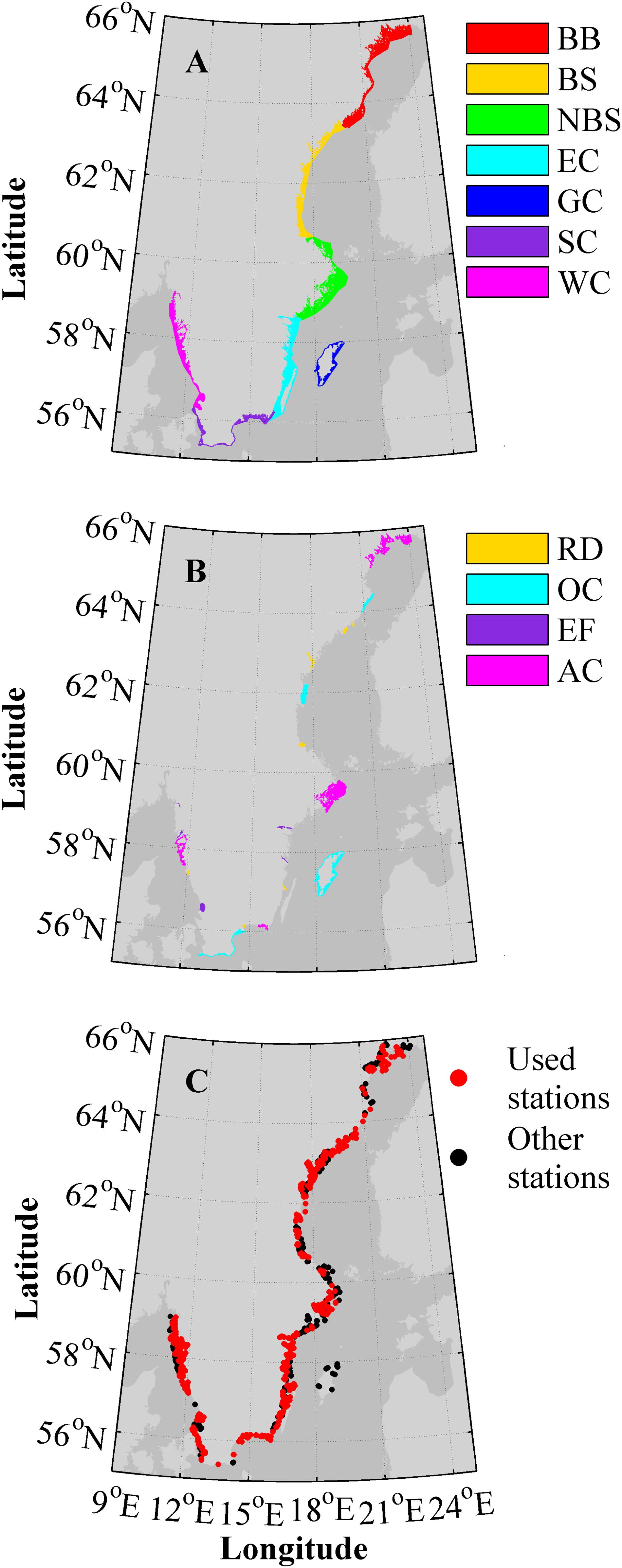
FIGURE 1. Maps of the Swedish coastline with abbreviations in the legends according to Table 1. (A) The seven major regions, i.e., the five water districts (WD1, WD2, WD3, WD4, and WD5) where WD4 is divided in three parts. (B) The key sites colored after type. (C) The coastal monitoring stations available in the SHARK database for the 1995–2014 period.

The present study will investigate retention efficiency, the coastal filter function and how it is related to environmental indicators along the entire Swedish coastline. The analysis will show how nutrient retention and some associated parameters vary along the coast, and also start to unravel which physical and environmental factors affect the retention in a water body. Understanding how effectively, and why, different coastal sites act as filter for land derived nutrients may help to upscale the results of more detailed studies at specific sites along the Baltic Sea coast.

This work was part of the BONUS COCOA project¹, which investigated the transports and transformations of nutrients in the coastal zone of the Baltic Sea.

Materials and Methods

To facilitate for the reader, the most frequently used abbreviations and definitions, including units, are listed in Table 1.

TABLE 1

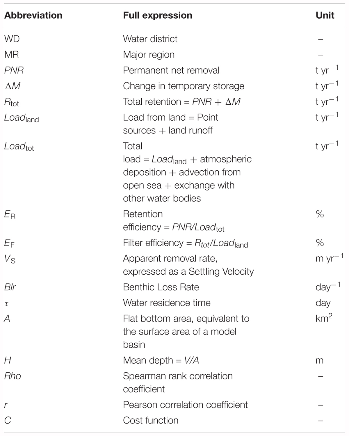
TABLE 1. List of abbreviations and units.

Retention

Retention is the withholding of matter within a region and is usually calculated as the external input to the area minus the export. This definition of retention includes both a withholding of matter but also internal removal or additions. To be able to set our results in a literature context we use the same definition in this study.

The approach described in the previous paragraph follows the concept of temporal and permanent retention introduced by Almroth-Rosell et al. (2016). They defined the total retention (R_tot) as the sum of permanent net removal (PNR, i.e., permanent retention) and changes in temporary storage (ΔM, i.e., temporary retention). PNR of nutrients is calculated from the models’ biogeochemical process rates, i.e., sinks and sources in the nutrient budgets. For phosphorus this only includes sediment burial while for nitrogen sediment burial, denitrification in water and sediment and fixation of dinitrogen (N₂) are included. The temporary retention is calculated as the annual change in nutrient storage in the water bodies, with the nutrient storage calculated as the sum of vertically integrated pelagic and sediment pools.

Retention Efficiency and Effective Coastal Filter

The retention discussed in Section “Retention” is expressed as annually retained tons of nitrogen and phosphorus. To better understand what these numbers entail they are set in relation to the load. We use both the total load (Load_tot) and the load from land (Load_land). Load_land is defined as the supply from rivers, surface runoff, groundwater and point sources. Load_tot is defined as the sum of Load_land, surface deposition, advective transports from the open sea and sound transports within the model domain. Note that the groundwater nutrient flux is not well known and thus, the groundwater output from the runoff model is difficult to estimate and also, as a consequence, to validate.

The retention efficiency (E_R) is the fraction of the total load that is permanently removed,

$$\begin{array}{c}{E}_{\text{R}} = \frac{PNR}{Loa{d}_{\text{tot}}}\left(1\right)\end{array}$$

The nutrient filter (the filter efficiency, E_F) is the retained fraction of land load only (from rivers, surface runoff, ground water and point sources)

$$\begin{array}{c}{E}_{\text{F}} = \frac{R_{\text{tot}}}{Loa{d}_{\text{land}}}\left(2\right)\end{array}$$

The filtering efficiency is calculated from the total retention since we are interested in estimating the long-term average nutrient filter around the Swedish coast, which should also include any possible long-term net effects of temporary retention. However, PNR is used to calculate E_R since the highly variable temporary retention (Almroth-Rosell et al., 2016) would be a hindrance in the following analyze.

Occasionally retention needs to be normalized to the horizontal area of water bodies or regions. This will be indicated in the text.

Theory of Steady State Retention

In order to understand what governs the retention efficiency in a specific water body we explore the concept of steady state retention as discussed in Eilola et al. (2017). For this we assume a well-mixed basin with a flat bottom with area (A) that is supplied with a bioactive tracer with the freshwater from land and with inflowing water from the adjacent sea. The bioactive tracer may be exported to the adjacent sea and also be removed due to PNR (Wulff and Stigebrandt, 1989). Especially, we investigate the functioning of PNR and retention efficiency in a case study where the bioactive tracer is a nutrient (nitrogen or phosphorus), which is also used for primary production of organic matter in a productive layer at the surface of the sea. Since we focus on shallow coastal areas we assume that the internal loss of the bioactive tracer mainly is due to permanent loss of nutrients in the sediment caused by, e.g., burial and/or denitrification.

The basis for the analysis is the mass conservation equation where changes in the pools depend on nutrient supplies, exports and the internal losses PNR. For simplicity, we investigate the steady state conditions where changes in the nutrient pools are assumed to be small. In accordance with Wulff and Stigebrandt (1989), we use the concept of an apparent removal rate, i.e., a fraction of the bioactive tracer mass in the water is removed with an apparent removal rate V_S. Thus, PNR within the system is dependent on V_S⋅C_pel⋅A, where C_pel is the mean pelagic nutrient concentration.

We use mass conservation

$$\begin{array}{c}V·\frac{d{C}_{\text{pel}}}{dt} = Q_0·C_0+Q_2·C_2 - Q·C_{\text{pel}}-PNR\left(3\right)\end{array}$$

and assume a steady state to calculate the concentration C_pel

$$\begin{array}{c}{C}_{\text{pel}}=\frac{Q_0·C_0+Q_2·C_2}{Q+V_S·A}.\left(4\right)\end{array}$$

Here V is the volume of water in the basin, dC_pel/dt the change in concentration of the nutrient with time (equal to zero in steady state), Q₀ is the freshwater supply from land and C₀ is the concentration of the nutrient in the inflowing freshwater (including here also the supplies from atmosphere and point sources), Q₂ is the inflowing water from adjacent basins, C₂ the concentration of the nutrient in the inflowing water and Q is the outflowing water.

The retention efficiency (Eq. 1) can be written as

$$\begin{array}{c}{E}_{\text{R}} = \frac{PNR}{Q_0·C_0+Q_2·C_2}\left(5\right)\end{array}$$

Using Eq. 4 this can be rewritten as

$$\begin{array}{c}{E}_{\text{R}} = \frac{1}{1+\frac{H}{V_S·\tau }},\left(6\right)\end{array}$$

where H = V/A is the mean depth and τ is the water residence time defined by:

$$\begin{array}{c}\tau = \frac{V}{Q}.\left(7\right)\end{array}$$

According to Eq. 6 E_R is a function of mean depth (m), water residence time (days) and apparent removal rate (m day^-1).

Since internal losses are assumed to take place mainly at the sea floor, the apparent removal rate (V_S) is related to the benthic loss rate, Blr (day^-1), in the sediment, i.e., PNR = V _S⋅C_pel⋅A = Blr⋅M_sed⋅A, where C_pel is the concentration in the water column (mmol m^-3). Thus, V_S can be expressed as a function of the mean vertically integrated mass in the sediment M_sed (mmol m^-2) and the C_pel (Eq. 8) for any bioactive tracer,

$$\begin{array}{c}{V}_{\text{S}} = Blr·\frac{M_{\text{sed}}}{C_{\text{pel}}}.\left(8\right)\end{array}$$

Here the benthic loss rate is related to the burial and denitrification rates, i.e., the deposition of bioactive tracer to the sediment and redox-state as well as the benthic release rate. It is dependent on many local factors such as the supplies to the sub-basin, the productivity and mineralization in the basin, which depend on the temperature, deep water stagnation, and potentially other factors.

Determining Dependence of E_R on Hydrological and Environmental Factors

According to the theory described in Section “Theory of Steady State Retention,” the retention efficiency of the coastal zone is determined by water depth and residence time as well as on the apparent removal rate V_S that depends on the environmental state in water and sediment. Previous studies (Nixon et al., 1996; Billen et al., 2011; Hayn et al., 2014; Almroth-Rosell et al., 2016) have shown the dependency only on hydrographical factors.

The modeled water bodies are of variable size and since PNR, and thus E_R, is largely determined by burial and denitrification, also the association strength to the sediment area of the water bodies will be investigated. E_R is calculated for each modeled water body according to Eq. 1 and residence times are derived from the model calculations (see section “Calculation of Residence Times”). Mean depths are calculated from the hypsography of the water bodies, i.e., total water volume divided by surface area.

To investigate the association strength between V_S and different environmental indicators, Eq. 6 is solved for V_S, i.e.,

$$\begin{array}{c}{V}_{\text{S}} = \frac{H·E_R}{\tau ·(1-E_R)}.\left(9\right)\end{array}$$

V_S can then be calculated for each water body. When V_S is known Blr can be calculated by solving Eq. 8 for Blr,

$$\begin{array}{c}Blr=V_{\text{S}}·\frac{C_{\text{pel}}}{M_{\text{sed}}}.\left(10\right)\end{array}$$

The environmental indicators that will be tested are: the ratio between the nutrient content in the sediment and in the water column (Eq. 8), the total nutrient content; the inorganic nutrients (dissolved inorganic nitrogen, DIN and dissolved inorganic phosphorus, DIP); N:P ratios; the hypoxic area; salinity; stratification strength; annual surface temperature and the effect of loads. The stratification strength is tested since it can indicate stagnant bottom water, hypoxic areas could be a proxy for denitrification rates, and DIN and DIP are often available from monitoring. DIN and DIP values are only taken from winter months, i.e., December, January and February. The selection of factors is a combination of what is given by theory, environmental factors that are known to have an impact on the environmental state and variables that are readily available.

The Coastal Zone Model System

The Swedish Coastal zone Model (SCM) is a multi-basin, one dimensional model based on the equation solver PROgram for Boundary layers in the Environment (PROBE; Svensson, 1998), coupled to the Swedish Coastal and Ocean Biogeochemical model (SCOBI; Marmefelt et al., 1999; Eilola et al., 2009). The model system was developed to calculate physical and biogeochemical states in Swedish coastal waters bodies. The set-up used in the present study includes 653 coupled basins covering the entire Swedish coast. The basins follow the water bodies defined by the water framework directive and mainly follow natural topographic constraints. The water exchange in the straits between the main water bodies is calculated from the baroclinic pressure gradients. The net flow through the sounds will be the same as the river discharge from land in order to preserve volume since the volume changes caused by precipitation and evaporation are neglected. The water exchange over the boundary between the coastal zone and the open sea is assumed to be in geostrophic balance, because normally this boundary is open with a width greater than the internal Rossby radius. The hydro-dynamical part of the SCM is integrated with high temporal resolution (10 min time step for hydrodynamics). Thus, changes in the physical characteristics, including, e.g., diurnal variations, freshwater and nutrient supplies, water exchanges and transports of substances between the sub-basins are resolved. The time step of the biogeochemical module (SCOBI) in SCM amounts to 1 h, which is sufficient to resolve biogeochemical sources and sinks in the sub-basins.

For this study, the model has been run for the 1985–2014 period. Below, the two main components of the model system, the forcing and set-up are described briefly. For more details the reader is referred to Almroth-Rosell et al. (2016) and other cited publications.

The PROBE Numerical Model

The physical model PROBE calculates horizontally averaged concentration profiles of all the state variables, including temperature and salinity. It calculates horizontal velocities, advection and mixing (Svensson, 1998). The surface mixing is calculated by a k–𝜀 turbulence model, light transmission as well as ice formation growth and decay are also included in the model. The vertical resolution is half a meter in the uppermost layers, 1 m in the 4–70 m interval, and 2 m between 70 and 100 m. Below 100 m the layer thickness increases to 5 m and to 10 m below 250 m. The general differential equation solved for each dependent, laterally averaged variable, ϕ, in each basin can be written as

$$\begin{array}{c}A\frac{\partial \varphi }{\partial t} = \frac{\partial }{\partial z}(A{\Gamma }_{\varphi }\frac{\partial \varphi }{\partial z} - Q_z\varphi )+q_{in}{\varphi }_{in} - q_{out}\varphi +A{S}_{\varphi }+\frac{\partial A}{\partial z}{J}_{\varphi bot}.\left(11\right)\end{array}$$

Here t is time, z vertical coordinate, A horizontal area, Γ_ϕ vertical exchange coefficient, S_ϕ source and sink terms per volume, J_ϕbot bottom flux per bottom area, Q_z vertical volume flux, and q_in and q_out horizontal volume fluxes per meter depth to and from the basin through connecting straits. From volume conservations the latter three variables are related through

$$\begin{array}{c}{Q}_z = {\displaystyle {\int }_{-H_{\max }}^z(q_{in} - q_{out})}dz\left(12\right)\end{array}$$

where H_max is the maximum depth of the basin. The sources and sinks determined by the biogeochemical model are added and subtracted from S_ϕ.

The SCOBI Model

The SCOBI model describes the dynamic biogeochemistry of marine waters (Eilola et al., 2009). Nine pelagic and two benthic variables are described in the SCM. In the pelagic zone, three different phytoplankton groups (diatoms, flagellates and others, and cyanobacteria), one zooplankton group, one pool for detritus and three inorganic nutrients pools (nitrate, ammonium, and phosphate) are represented. The model also calculates oxygen and hydrogen sulfide concentrations, which are represented by “negative oxygen” equivalents (1 ml H₂S l^-1= -2 ml O₂ l^-1) (Fonselius and Valderrama, 2003). For the benthic layer the amounts of stored nitrate and phosphate are calculated. SCOBI has been used and validated in several studies, both coupled to the PROBE-Baltic (Marmefelt et al., 1999) and to the three dimensional Rossby Center Ocean model (RCO; e.g., Meier et al., 2011).

Burial, denitrification and N₂-fixation are the processes that affect the permanent retention in the model. The burial is parameterized from the concentration of nutrients in the active sediment layer (i.e., approximately 2–5 cm) and a burial rate constant that defines how large a fraction of the sediment nutrient content (mmol/m²) that is to be buried in each time step. A burial constant is set for each water district. There is an additional burial of nitrogen due to a small amount of N-adsorption to sediment particles. For nitrogen, also denitrification contributes to the permanent removal. On the other hand, N₂-fixation adds organic N to the system in favorable conditions (i.e., a salinity below 10 and low N:P ratios, not active on the West Coast) and thus counteracts the removal of nitrogen, i.e., N₂ fixation causes negative retention of nitrogen. Denitrification is incorporated in the model in both the free water mass and in sediments. The pelagic denitrification is regulated by the redox state of water and the availability of nitrogen, while the benthic denitrification is regulated by bottom water oxygen concentrations and sediment nitrogen regeneration/mineralization.

One should note that the assimilation of nutrients taking place at the seafloor on illuminated sediments could affect water-sediment fluxes (Hoefsloot, 2017), and thus retention, but this is not yet explicitly described in the SCM.

For further details of the SCOBI model the readers are referred to Eilola et al. (2009); Almroth-Rosell et al. (2011), Eilola et al. (2011), and Almroth-Rosell et al. (2015).

Model Forcing

The SCM-SCOBI model system is forced by weather, atmospheric deposition of nutrients, the conditions in the sea outside the coastal zone, and discharge of freshwater and nutrients from land. The initial values for both the pelagic zone and the sediment are derived from spin-up simulations.

The weather variables are taken from the gridded Lars Mueller database (3-hourly meteorological synoptic monitoring station data) at the Swedish Meteorological and Hydrological Institute (SMHI) up until 2010. After that the forcing is based on MESAN model output (Hāggmark et al., 2000). The insolation and all the radiation and heat fluxes across the water-air interface are calculated by the PROBE model. Atmospheric depositions of nitrogen species (NHX and NOX) are a climatic estimate based on a 3 year simulation (2001–2003) by the MATCH model (Robertson et al., 1999). For the deposition of phosphate a literature value of 0.5 mg m^-2 month^-1 is used (Areskoug, 1993).

Observations alone are inadequate to force the models open Baltic Sea and Kattegat boundaries since the temporal resolution is too low (monthly) and the information is incomplete (e.g., lacking information on zooplankton, phytoplankton and detritus). Hence, the lateral boundary of the outer archipelago to the open Baltic Sea is set by vertical mean profiles calculated by 1D PROBE set-up for each open sea area including assimilation of monitoring data.

The land derived forcing is divided in two types; discharge of water and nutrients as well as point sources representing sewage plants and industries. The discharge is given by the S-HYPE model (Lindstrom et al., 2010) and consists of river water, ground water and surface run-off from the drainage area surrounding each coastal basin. No reduction of river nutrients due to retention at river-mouths is assumed in this model setup. The loads from point sources mainly consist of nutrient loads reported in VISS² and data collected via personal communication with local and regional management boards to enhance time resolution for larger sewage plants. Thus, the loads from the point sources have varying time resolution.

Model Output Treatment

Model Skill Evaluation

Since the sub-basins of the model are horizontally averaged and the model system is forced by coarse-resolution weather and boundary conditions that may deviate from the actual situation, it is not realistic to expect reproduction of detailed synoptic features or patchy properties in the model results. Instead we focus the evaluation on averaged modeled and measured values during 1996–2014. To capture the characteristics of the basins we look at vertical profiles and seasonal cycles of salinity and the biogeochemical parameters in the surface and deep waters. Salinity represents the general circulation in the coastal zone and biogeochemical cycling is evaluated by nutrients and oxygen in the deep water while nutrients and salinity are evaluated in the surface water.

Since many monitoring stations in the coastal zone have poor data coverage either in the vertical or in time, a sub-set of the model results are extracted to represent the timing and vertical/annual location of the monitoring data. Model data is extracted for a week (±3 days) around any time of measurement and for ±3 m vertically around the measured depths. This allows for the usage of scarce monitoring data and still keeping the model output comparable. Observational data from all stations in a water body have also been combined to give better observational data coverage. Using several stations from different location also shows the horizontal range that can occur within a water body, which reduces the problem of comparability that can occur if only one monitoring station being placed in the outskirts of a water body is used.

The observational data used for validation are open access and extracted from SHARKweb³. The used stations are indicated in Figure 1C. The quality flags included in the data base output have been used to exclude data that the data host does not trust, e.g., values flagged as bad or suspected.

To give an overview of the model skill in the just over 200 basins included in the evaluation and avoid relying only on subjective visual inspection of the results, two dimensionless skill metrics, the Pearson correlation coefficient (r) and the mean of a cost function (C) (Eilola et al., 2009) are used (Eq. 13 and 14).

$$\begin{array}{c}r=\frac{{\displaystyle {\sum }_{i=1}^n(P_i - \overline{P})}(O_i - \overline{O})}{\pm \sqrt{{\displaystyle {\sum }_{i=1}^n{(P_i - \overline{P})}^2}}{\displaystyle {\sum }_{i=1}^n{(O_i - \overline{O})}^2}}\left(13\right)\end{array}$$

$$\begin{array}{c}C=\frac{{\displaystyle {\sum }_{i=1}^n\left|\frac{P_{\text{i}} - O_{\text{i}}}{sdt(O_{\text{i}})}\right|}}{n},\left(14\right)\end{array}$$

where i is the depth level or seasonal point in time in the vertical profiles or seasonal variations, respectively. The correlation coefficient compares the similarity in the shape of the vertical profiles and seasonal cycles between measured data (O_i) and model results (P_i) by evaluating the Pearson correlation (Eq. 13). The mean cost function value indicates the proximity of the model to measurements by normalizing the off-set between them with the standard deviation of the observations. If the average model results fall within the standard deviation of what is observed, C will be below one. For two data sets with identical shape, r will be 1 and if there is no correlation, r has values around zero. Similar approaches has previously been used in Edman and Omstedt (2013) and Edman and Anderson (2014) and is based on the recommendations given by Oschlies et al. (2010). The normality of the observational and model data-sets has been evaluated with the Lilliefors test (Lilliefors, 1967).

The estimation of r is problematic if the data distribution is too homogeneous, e.g., a well-mixed water body would give a straight vertical salinity profile without much spread in data and thus, make the analysis sensitive to any small, insignificant differences between the observed and modeled output distributions. Likewise, if the standard deviation of observed data is low, e.g., nutrient concentrations in summer surface waters are often below or close to the detection level and are thus set to the same default low values, the calculation of C becomes very high. Both situations would give indications of bad quality even if the actual problem would not be the model but the evaluation technique combined with the inherent quality of the data sets. Thus, for r computations the maximal spread in averaged observational data is set to be at least 10% of the average concentration of both model results and observations. For C, the standard deviation of observational data has to be at least 10% of the average concentration calculated from both model and observations, for the computation to be done.

Averages of the measured data have been calculated for occurrences of dense data distribution during the year and vertically, and the model output has been averaged for the same time and depth ranges. The evaluation has been performed for depth profiles of salinity (S), DIN, DIP, oxygen (O₂), seasonal surface variation of DIN and DIP as well as the bottom annual variation of O₂. For all vertical profiles the evaluation has been volume weighted so that more relevance is assigned to the accuracy in the large surface volumes of the water bodies.

Clustering of Water Bodies

Not all properties are valid or valuable to be calculated for individual water bodies, for example the coastal filter only makes sense to be calculated for a larger area that participates in the filtering of land load from rivers. Hence, besides calculating average results for the individual water bodies and for the entire coast, two more approaches are used in this study.

The first approach is to analyze the model results clustered together in seven major regions (MRs) (Figure 1A and Table 1): the Bothnian Bay coast (WD1, BB), the Bothnian Sea coast (WD2, BS), the Northern Baltic Sea coast (WD3, NBS), the East Coast (WD4, EC), the Gotland Coast (WD4, GC), the South Coast (mainly Skåne) (WD4, SC) and the West Coast (WD5, WC). The division is based on the five water districts that are used in Swedish coastal management and related to the different characteristics of the off shore water bodies. As described above, WD4 is divided into three parts; Gotland, Skåne and the rest of the east Swedish coast up to water district three. This approach should capture major differences or gradients along the coast, mainly based on off shore conditions, but also influenced by freshwater properties draining into each major area.

To investigate the influence of coastal type and freshwater conditions, the second approach is focused on specific key sites based on the coastal environments proposed in the BONUS COCOA project. The sites have been selected manually to give a few sites representing each of the coastal environments: archipelagos (AC), river dominated (RD), open coast (OC), or embayments, mainly fjords (EF) (Figure 1B and Table 1).

Calculation of Residence Times

The residence time is the average time that a water parcel resides within a defined water volume. In the present study, the residence time is calculated in three different ways:

(1) For the individual water bodies, i.e., the model basins, the average water age is calculated by the model using a concept that is described in detail by Engqvist et al. (2006). The values used in this study are the 20-year vertical volume weighted averages. Since the basins are calculated as horizontally homogeneous, the age can be used as a measure for the residence time because residence time (or average transit time) and average age are identical in case of well-mixed reservoirs, i.e., reservoirs that contain water parcels of all ages (Bolin and Rodhe, 1973).

(2) For larger clusters, containing several model basins, the equality between water age and residence time is no longer valid and we calculated the residence time as the total water volume in the cluster divided by the total outflow.

(3) To compare the filter efficiency calculated in this study to literature values, a third approach is applied where the freshwater residence time (τ_qf) is calculated as the freshwater volume in a cluster divided by the freshwater inflow it receives. This method follows the freshwater fraction method discussed by Sheldon and Alber (2006). A freshwater tracer is used to determine the freshwater volume. The filter efficiency refers to the filtering of nutrients carried by freshwater and thus, the flushing of the freshwater fraction is the relevant residence time.

Association Strength of Retention With Ambient Factors

To understand which factors that determine the retention in the coastal zone, the strength of association between nutrient retention and several ambient variables needs to be tested. However, the null hypothesis that retention values in the water bodies are normally distributed was rejected by a Lilliefors test (Lilliefors, 1967) thus, we cannot use the common Pearson correlation. Instead, the Spearman rank correlation will be used to evaluate association strength. The correlation coefficient is denoted Rho. The Spearman rank correlation, or Spearman’s Rho, does not require normally distributed samples and it also evaluates the monotonic relationship between two data-sets rather than their linear relationship. Since the association between the nutrient retention and ambient variables is not necessarily linear, the evaluation of monotonic relationships, i.e., the values should have a strict increase or decrease in the data-set, is better for this evaluation. A limit of p < 0.05 is used to determine significance.

Results

Model Skill Evaluation

The model skill averaged over salinity, DIN, DIP, and oxygen, expressed as C and r, is acceptable in all water districts (Figure 2, numbers colored after WD). However, at the Bothnian Bay coast (WD1) the data coverage is still poor and thus it is hard to evaluate the model quality with any certainty, especially for oxygen. When the variables are evaluated separately within the WDs (Figure 2, colored markers) the averaged salinity bias in the north (i.e., WD1 and WD2) is not within two standard deviations of the measurement data, i.e., not acceptable. Neither is the model’s skill to simulate oxygen in WD3. All other variables are simulated with an acceptable skill.

FIGURE 2

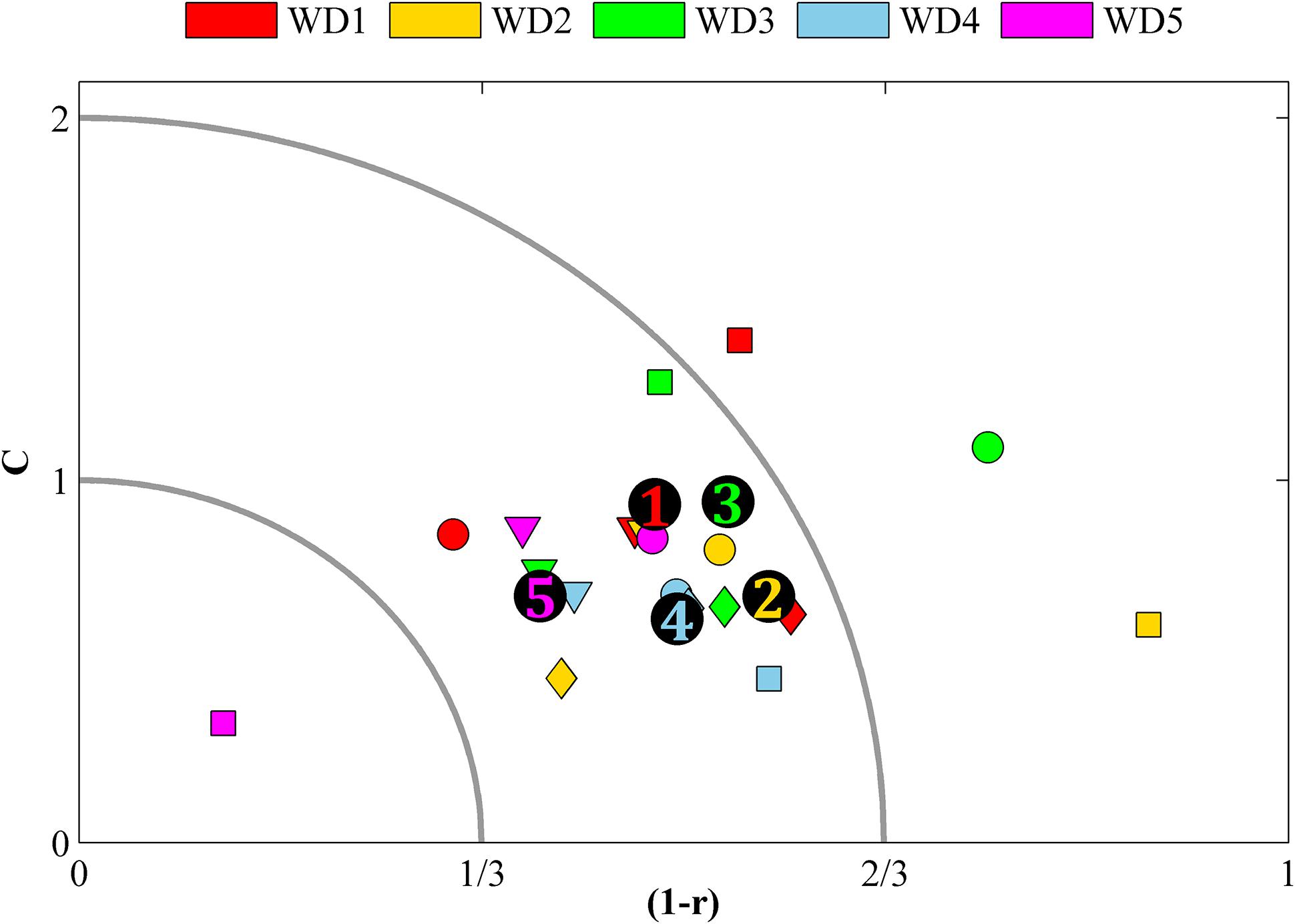
FIGURE 2. Model bias shown as combination of correlation bias (1–r) and mean bias C in the five WDs. Colored markers denote the averaged bias for a single variable (square = salinity, round = oxygen, diamond = DIN and triangle = DIP) in a WD. Numbers mark the average bias in a water district (all variables included). Markers inside the outer quarter circle has a combined C and 1–r bias that indicate that the model skill is acceptable and markers within the inner quarter circle indicate good model skill. Markers outside the quarter circles indicate too large biases.

However, for specific basins (not shown) the results are sometimes very poor (or very good). Especially the shape of nutrient distributions, represented by (1-r), compares poorly to what is observed in some basins. It is mainly the vertical correlation that causes too large biases (not shown). However, for this study it is more important that the levels are right, which is indicated by the C-values, and for the nutrient distributions only five basins have biases that are not acceptable (not shown). The averages shown in Figure 2 are all good or acceptable with regard to C in all water districts.

Overview of Land Loads, Physical Characteristics and the Temporal Variability of the Coastal Nutrient Pool

The averaged mean depth in the water bodies along the coast (Figure 3A) is about 20 m but ranges from 0 to 60 m. The shallow areas are typically close to the coast, in fjords and bays, with some exceptions such as the deep Gullmars Fjord on the West Coast and parts of the Stockholm archipelago. The deepest locations are found in the northern parts of the Swedish West Coast and outer rim of the Bothnian Sea coast. Also locations in the outer part of the Stockholm archipelago and the northern tip of Gotland have relatively large mean depths.

FIGURE 3

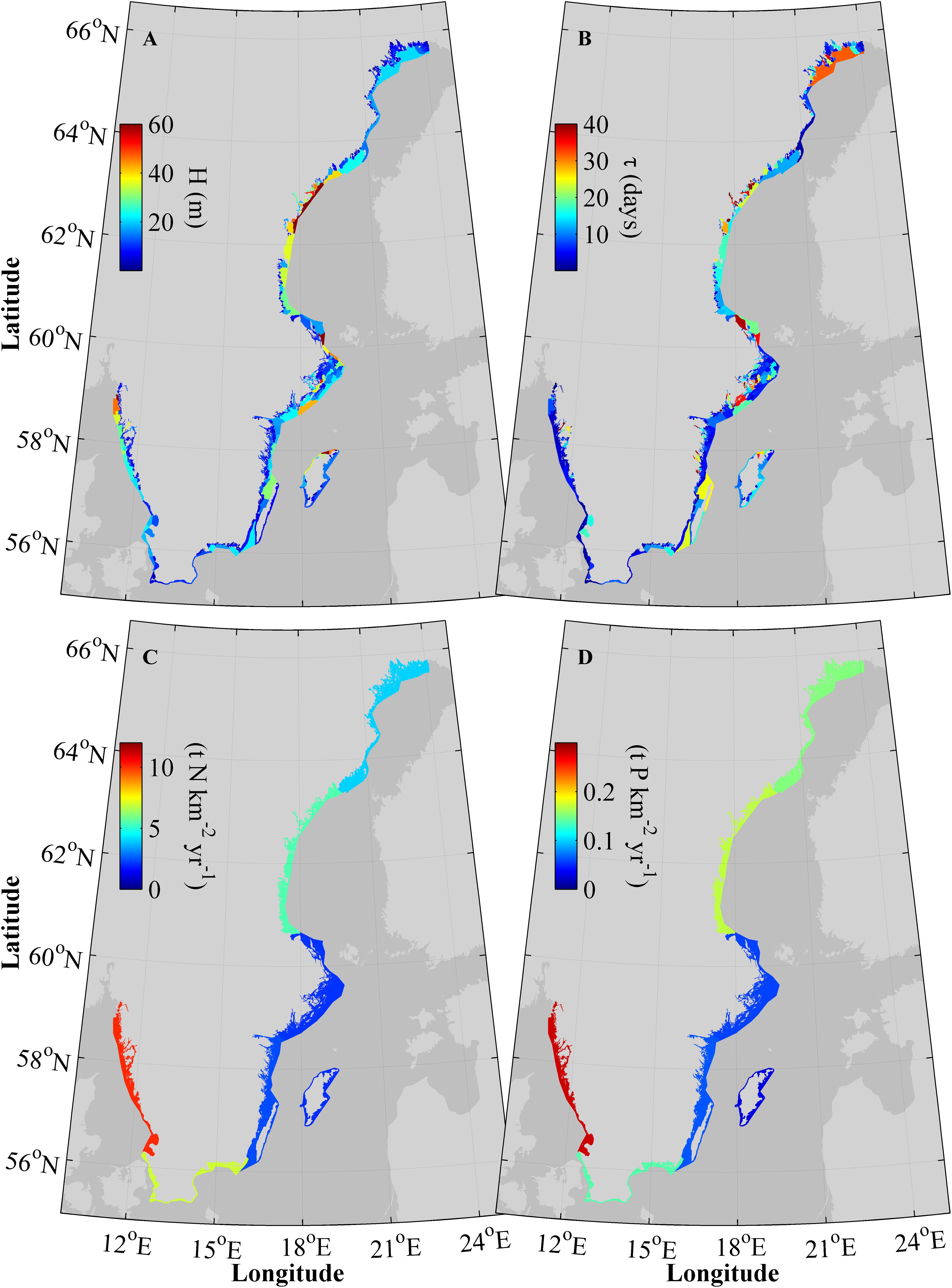
FIGURE 3. Mean depth, H, (A) and average age, τ, (B) for the individual water bodies along the coast, and land load (S-HYPE and point sources) normalized to area (C,D) for the seven MRs.

Residence times in the model (Figure 3B) are most commonly between 1 and 10 days and tend to co-vary with the mean depth, i.e., deeper basins tend to have longer residence times. However, there are exceptions, e.g., the northern part of the West Coast where the residence times in the outer part of the coastal zone are comparable to the averaged residence time in WD1, even if the area is very deep. Some of the more open areas between the mainland and the Öland Island, as well as the outer waters of the Bothnian Bay coastal stretch, have residence times of up to 25–30 days, while the shallow inner areas of the coastal zone can have either very short residence times of as small as 1 day or less, or up to 30–40 days.

The nutrient load normalized to the areas (Figures 3C,D) shows that the relative load is lowest to the south-east Swedish coast, especially Gotland. The pressure of anthropogenic nutrients is highest at the West Coast followed by the Bothnian Bay. Almost one third of the nitrogen (32%) and phosphorus (29%) from land and air to the Swedish coastal zone is discharged to the West Coast (not shown). The spatial distribution of the normalized nitrogen and phosphorous loads are similar. The normalized load ranges between 0.1 and 10 t nitrogen per km² and 0–0.3 t phosphorus per km², annually.

The development of the nitrogen and phosphorus pools over the 30 years of the model run is illustrated in Figure 4. The phosphorus pool decreases on the west and south-eastern coastal stretches but increases in the coastal zone bordering the Bothnian Sea. At the Bothnian Bay and the Northern Baltic proper coasts, the pool at the end of the run is very similar to the initial values in 1985. However, in both areas the values decrease in the period in between and then rise again in recent years. The recent increase in the modeled pools is most likely due to increased phosphorus content in the open sea forcing. For nitrogen, the general patterns are the same as for phosphorus, but for individual years the behavior of the nitrogen and phosphorus pools differs.

FIGURE 4

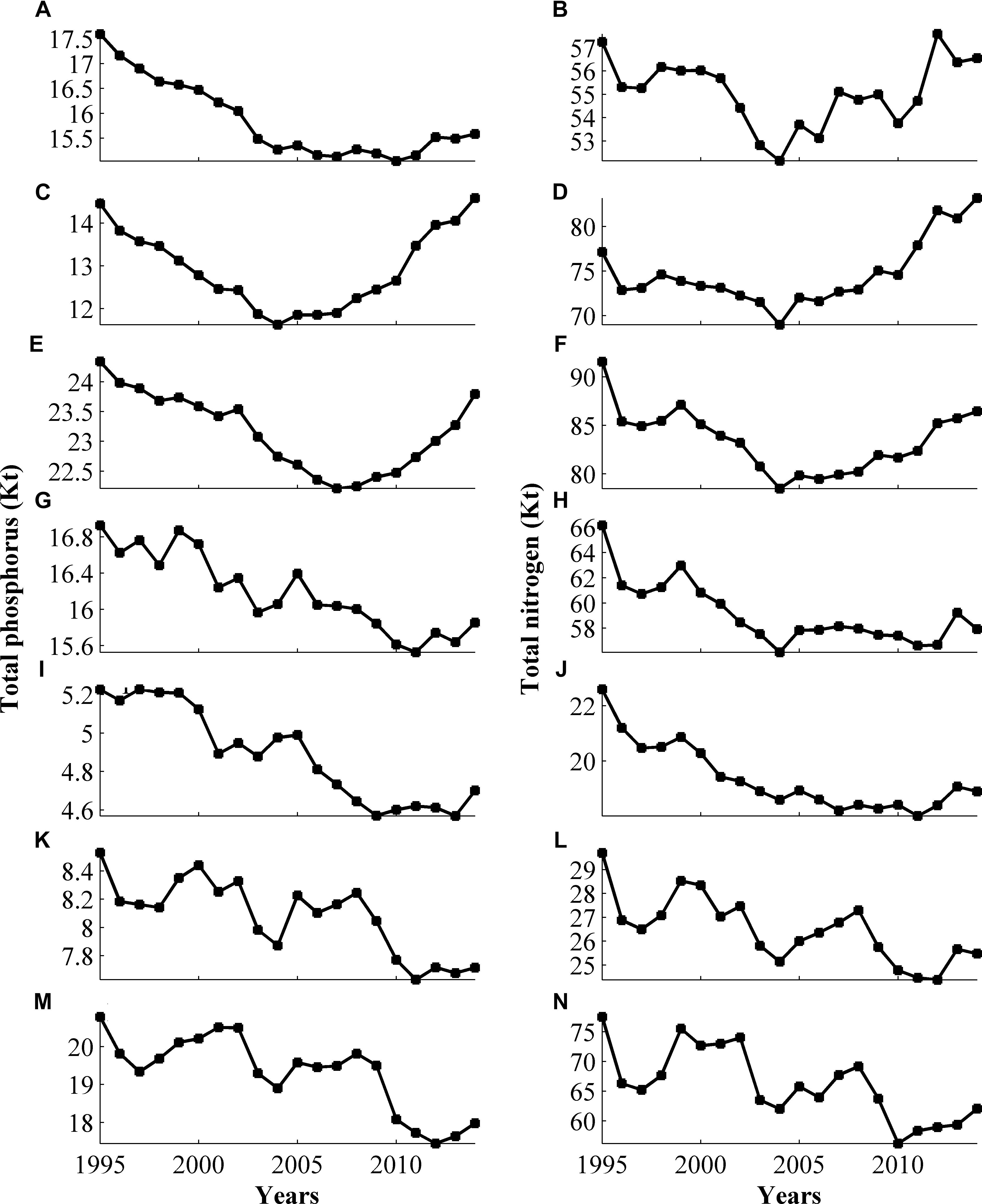
FIGURE 4. Annually averaged nutrient reservoirs in the Bothnian Bay (A,B), the Bothnian Sea (C,D), the Northern Baltic Sea (E,F), the East Coast (G,H), Gotland (I,J), the South Coast (K,L), and the West Coast (M,N), expressed in Kt. The reservoir is the sum of the vertically integrated pelagic and benthic nutrient in dissolved inorganic, and organic and particulate organic forms.

Estimations of the Coastal Filter Efficiency

The filter efficiency of nitrogen and phosphorus in relation to the depth to residence time ratio (H/τ_qf) is shown in Figure 5. This relation has previously been used in earlier studies (Nixon et al., 1996; Billen et al., 2011; Hayn et al., 2014; Almroth-Rosell et al., 2016). The present study adds the entire Swedish coast, the seven MRs and the smaller key sites. Most of the key sites and MRs investigated in this study have the same dependence on H/τ_qf as seen in previous studies. The association is negative and the range is rather wide. The range depends on the different environmental conditions of the studied areas.

FIGURE 5

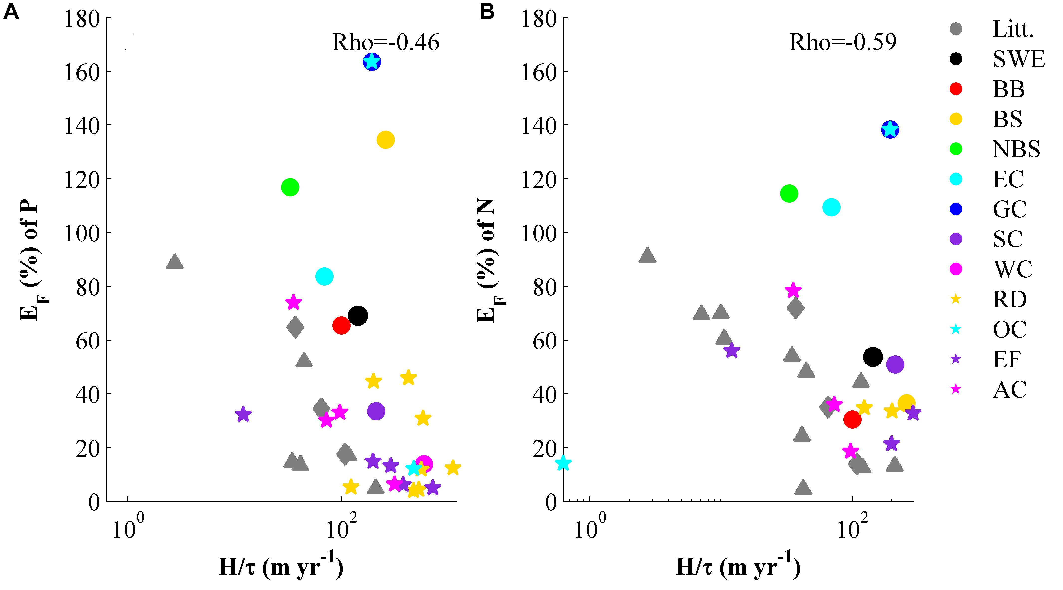
FIGURE 5. Filter efficiency, E_F, of phosphorous (A) and nitrogen (B), versus the ratio between the depth and the residence time (H/τ). The literature data (gray triangles) are from Nixon et al. (1996); Billen et al. (2011), Hayn et al. (2014) and the gray diamonds are values from Almroth-Rosell et al. (2016). The colored dots and stars are from this study (abbreviations in the legend according to Table 1).

Retention, Retention Efficiency and Filter Efficiency in the Swedish Coastal Zone

The average, annual retention for the Swedish coast is approximately 71 Kt nitrogen and 2.9 Kt phosphorus (Table 2). The nutrient filter capacity of the entire Swedish coast is estimated to be about 60% (approximately 53% for nitrogen and 69% for phosphorus) and thus, less than half of the input from land can be assumed to be exported from the coastal zone to the open sea. However, the differences between the water districts are large. The lowest filtering of land nitrogen occurs in the coastal zone of the Gulf of Bothnia while the lowest phosphorus filtering is calculated for the Swedish West and South Coasts. The Gotland Coast, WD3 including the Stockholm archipelago, and the East Coast in WD4 all retain more than 100% of the land and air load they receive. Thus, these areas have a net import and retention of open Baltic Sea nutrients and filter not only the land load but also the Baltic Sea water.

TABLE 2

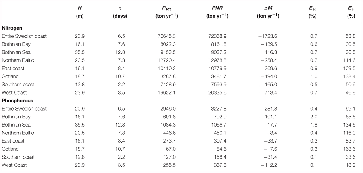
TABLE 2. Averaged (1995–2014) depth (H), residence time (τ), total retention (R_tot), permanent net removal (PNR), temporary changes in nutrient storage (ΔM), retention efficiency (E_R) and filter efficiency (E_F) in the seven major regions.

The total retention is divided in temporary retention, i.e., the nutrient storage changes in the coastal zone, and the permanent retention caused by net removal of nitrogen through denitrification and permanent burial in sediments (Table 2). For the modeled period the permanent retention is always positive but the temporary retention is negative for all areas except the Bothnian Sea coast.

However, the absolute value of the long term temporary retention is almost always smaller than the long term permanent retention and as a consequence, the total retention values are positive. The only exception in this study is a stretch of open coastline in the south of Sweden (Table 3, key sites) where the total retention of phosphorus is negative. For nitrogen the temporary retention is typically 1–2 orders of magnitude smaller than PNR. For phosphorus, the values are typically one order of magnitude smaller, only occasionally are they of the same order of magnitude as PNR. Thus, the total retention of phosphorus is more affected by the negative temporary retention than nitrogen.

TABLE 3

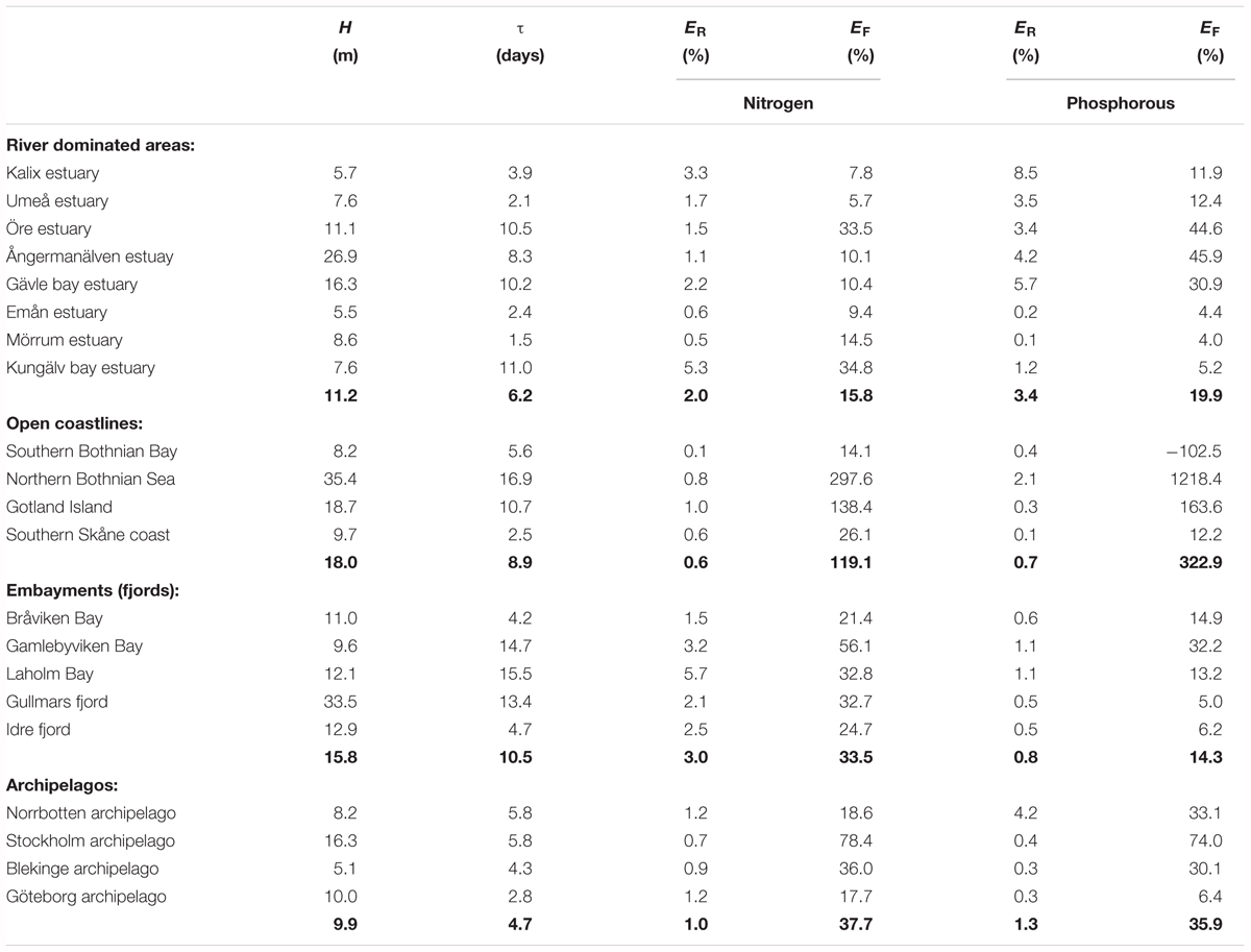
TABLE 3. Averaged (1995–2014) depth (H), residence time (τ), retention efficiency (E_R) and filter efficiency (E_F) at the key sites, with averages for each coastal type in bold numbers.

The 20-year average nutrient retention in individual water bodies range between approximately 0–0.25 t P km^-2 and 0–7 t N km^-2 annually for phosphorus and nitrogen, respectively (Figure 6). In Figure 6, the nutrient retention has been normalized to the sediment areas of the water bodies to avoid that their different sizes affects the visual impact of the results. The nitrogen retention is highest on the west coast and in certain near shore basins on the east coast, e.g., water bodies in the inner Stockholm archipelago. Phosphorus retention is highest along the Bothnian Sea shore, especially in the water bodies bordering the Baltic Sea. Overall, the phosphorus retention is high in some near shore protected bays but not in all such locations. There is also a tendency that low retention of both nutrients occurs in basins in-between the open Baltic Sea and the inner bays and estuaries.

FIGURE 6

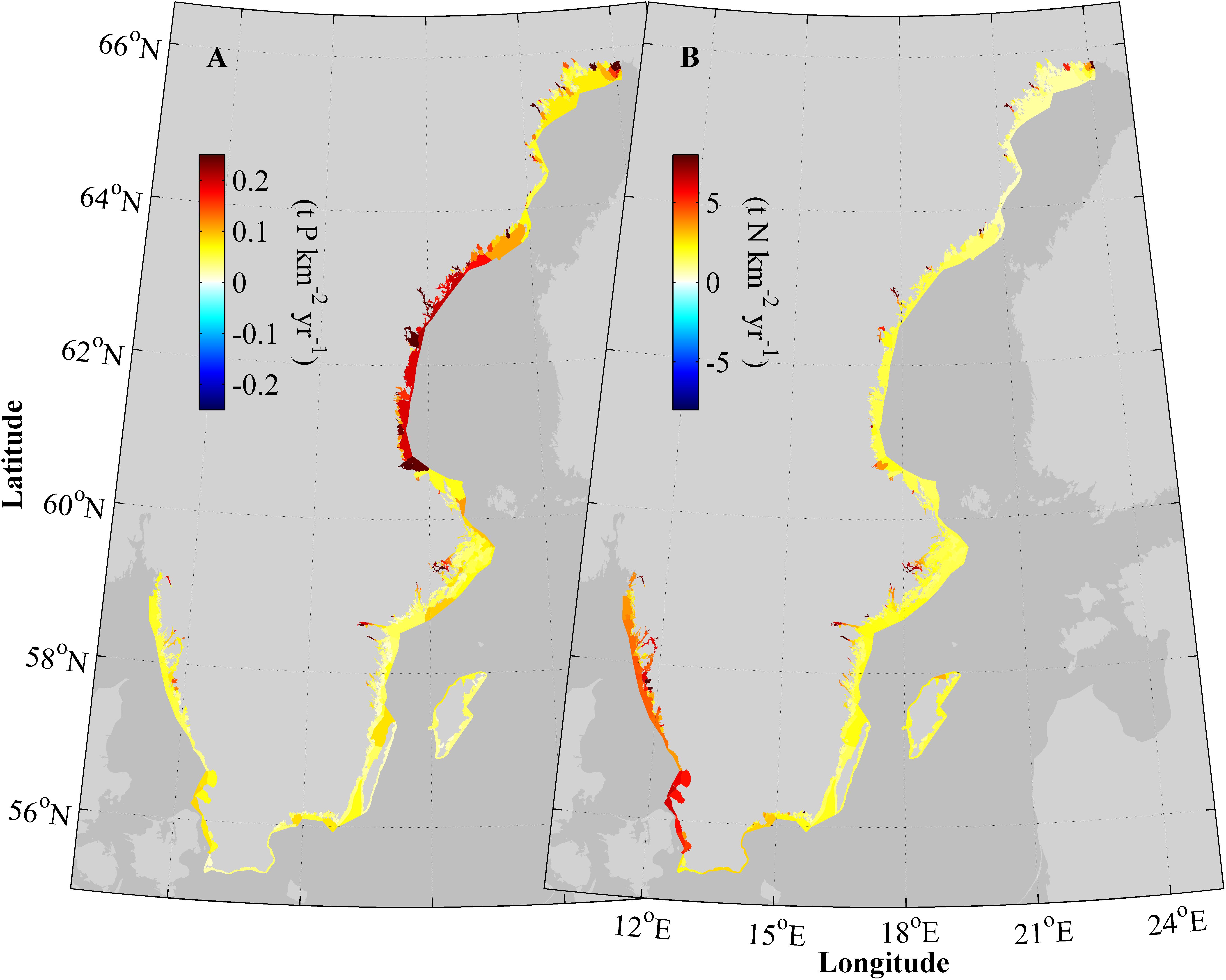
FIGURE 6. A 20 years average (1995–2014) of total retention, R_tot, of phosphorous (A) and nitrogen (B) normalized to area and in all modeled water bodies.

The retention efficiency, i.e., the percentage of retained total load, in the individual water bodies in the Swedish coastal zone, shows the same general spatial patterns for both nutrients (Figure 7). The nutrient removal is most efficient close to land, in bays, fjords and archipelagos.

FIGURE 7

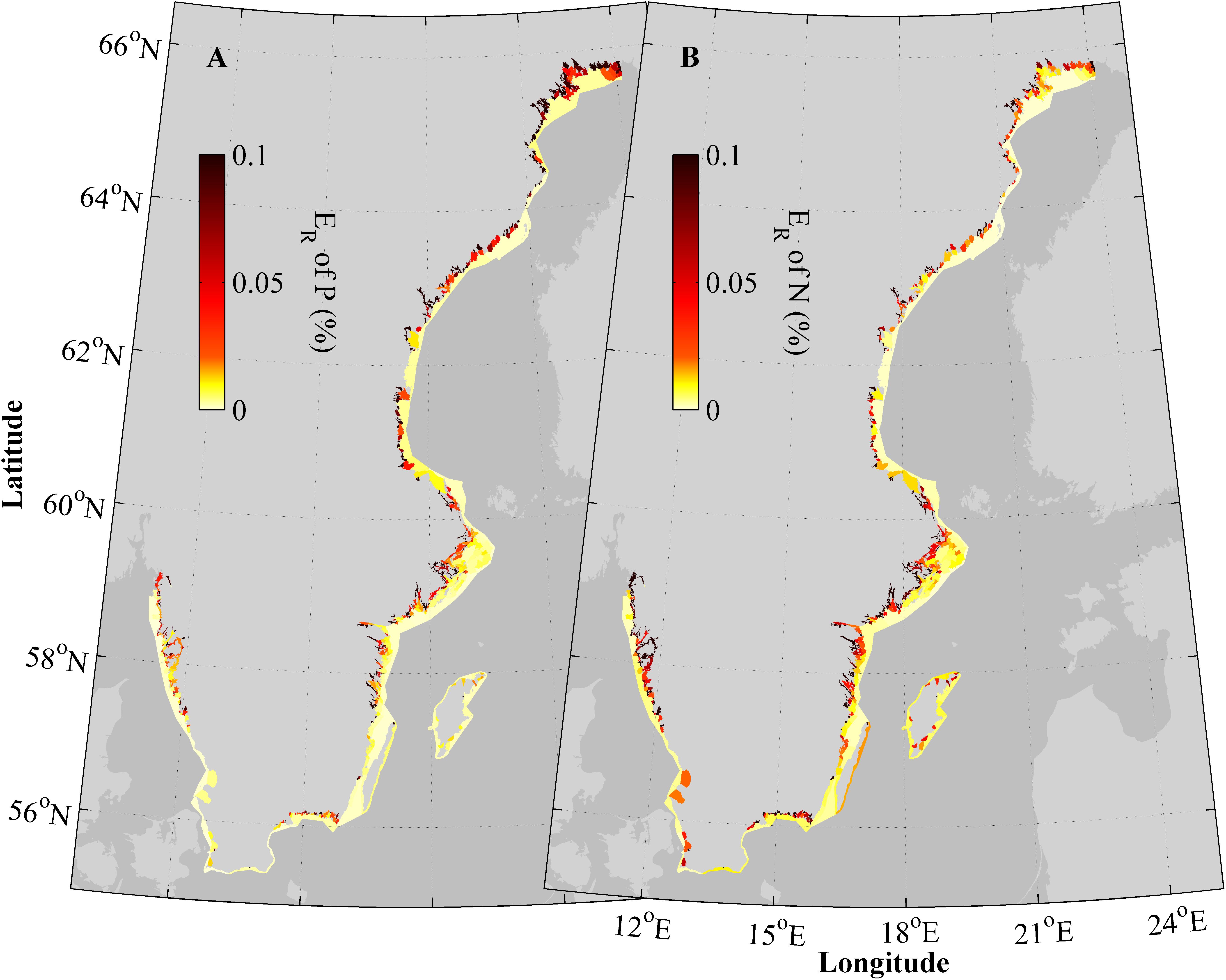
FIGURE 7. A 20 years average (1995–2014) of total retention efficiency, E_R, of phosphorous (A) and nitrogen (B) in all modeled water bodies.

Filter Efficiency at Key Sites

Judging from the average values from each type of area, archipelagos and open coastlines tend to be the most effective nutrient filters (Table 3). However, due to the large variability within each coastal type this result does not give strong support to any general patterns of filter efficiency. For open coastlines, the averaged E_F is over 100% and for archipelagos, 36 and 38%, for phosphorus and nitrogen, respectively. River dominated areas without archipelagos have slightly lower filter capacity (20% phosphorus and 16% nitrogen), but the variability is large. For embayments the filter is usually more efficient for nitrogen, while the other coastal types show no difference between the nutrients.

The most effective river dominated site is the Öre estuary where approximately 33–45% of the nutrients from land are retained or removed in the coastal zone close to land. These are higher percentages than calculated for the Norrbotten and Göteborg archipelagos. The high values for the open coastlines are an effect of extremely high values for the northern Bothnian Sea coast.

Temporal and Permanent Components of Total Nutrient Retention

This section describes how the modeled total retention (R_tot) is associated to temporal storage (ΔM) and PNR and also how these two components relate to each other. In Figures 8A,B each small colored dot represents 20 annual averages within a basin. The squares in the same figures represent data-sets of a 20-year average from each basin within a larger area. The squares thus show how the average R_tot is associated to averaged ΔM and PNR within either an MR or the entire Swedish coast.

FIGURE 8

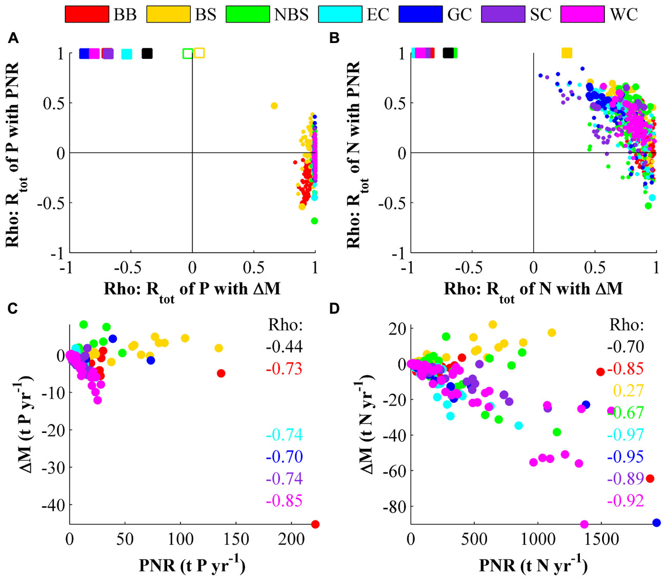
FIGURE 8. Association strength (Spearman’s rank correlation, Rho) of total retention (R_tot), internal losses (PNR) and changes in nutrient storage (ΔM). (A,B) Each marker represents a data-set for which the association strength of R_tot to PNR and ΔM has been calculated. The correlations in data-sets consisting of inter-annual variations within basins are shown as colored dots and correlation of 20-years averages are shown as colored squares. Smaller dots and open or missing squares denote that the correlation was insignificant (p > 0.05) for one correlation coefficient. (C,D) Show 20-year averaged values from each basin. Statistically significant (p < 0.05) Rho values are printed in the figure.

Long-Term Average Retention

The average R_tot (Figures 8A,B, colored squares) is very strongly associated to PNR. This was expected and agrees with previous result in Almroth-Rosell et al. (2016) and Section “Estimations of the Coastal Filter Efficiency” in this paper where it is stated that the average PNR is usually at least one order of magnitude larger than the absolute average ΔM. The association of the average R_tot to ΔM is instead negative with the exception of the Bothnian Sea and northern Baltic Sea coasts. Neither of the latter coastal stretches seem to have any association (open squares in Figure 8A) between R_tot and ΔM for phosphorus. The Bothnian Sea coast has a positive association between R_tot of nitrogen and ΔM (yellow square in Figure 8B), contrary to all the other investigated regions. This gives that the average R_tot within a water body is usually determined by its PNR rate, but also that water bodies with less changes in nutrient storage are more likely to have a high total retention, but the cause for this is not yet determined. It was also found (not shown) that a system with a higher total load tends to have a lower, most likely negative, average temporary retention compared with systems with a lower total load. This may be caused by load reductions from large point sources during the investigated period and thus, it is not a generally applicable result.

Interannual Variability of Retention

On inter-annual timescales (Figures 8A,B, colored dots) the total retention in a water body is generally associated with ΔM, in contrast to the results in Section “Long-Term Average Retention.” This result is in agreement with Almroth-Rosell et al. (2016). For phosphorus the association is very strong for all basins but for nitrogen the association is insignificant at some locations, especially around Gotland (blue dots) and the South Coast (purple dots). These basins with low inter-annual association of R_tot to ΔM tend to have stronger inter-annual association of R_tot to PNR instead. This gives that annual fluctuations of R_tot within a water body are most likely caused by changes in the amount of nutrient it holds. However, for nitrogen there can also be an influence of an increased removal rate (i.e., increased denitrification or burial). On inter-annual timescales a majority of the modeled water bodies tended to have a positive temporary retention if the load increases to a basin (not shown).

The Impact of Sediment Area on Permanent Retention

Changes in a water body’s nutrient content are usually negatively associated to PNR within the MRs (colored Rho values in Figures 8C,D), but for the coast as a whole, the association is weaker than for the individual regions. It is likely that the negative association between ΔM and PNR is caused by both being associated to the size of the water bodies. The correlation between PNR and sediment area is strong (not shown) with Rho of 0.89 for both phosphorus and nitrogen. The results are clearly grouped after water district and the correlation is stronger when the association is evaluated separately for MRs. The differences between the water districts are caused by the use of different burial rate constants. ΔM is negatively associated to the sediment area (A) (not shown), i.e., smaller water bodies tend to have larger fluctuations in their nutrient storage. The correlation of ΔM with A is strong for most MRs, with the exception for Bothnian Sea coast and the northern Baltic Sea coast were the association was weak or slightly positive. The resulting association of ΔM with A for the coast as a whole is -0.50 and -0.63 for phosphorus and nitrogen, respectively.

Estimating Retention Efficiency From the Physical Characteristics of Water Bodies and Environmental Indicators

The retention efficiency (E_R) does not have strong association to a water body’s surface area (Figures 9A,B), even if PNR does. Instead E_R is positively associated with τ (Figures 9E,F) and also negatively associated with H (Figures 9C,D), even if the latter association is weaker. When the two properties are combined as τ/H or according to Eq. 9, the correlation increases (Figures 9G–J) with a Rho of 0.71 and 0.75 for phosphorus and nitrogen, respectively. The use of Eq. 9 does not strengthen the association for either of the nutrients (Figures 9I,J) in comparison with the simpler expression τ/H. This is true also when the MRs are evaluated separately.

FIGURE 9

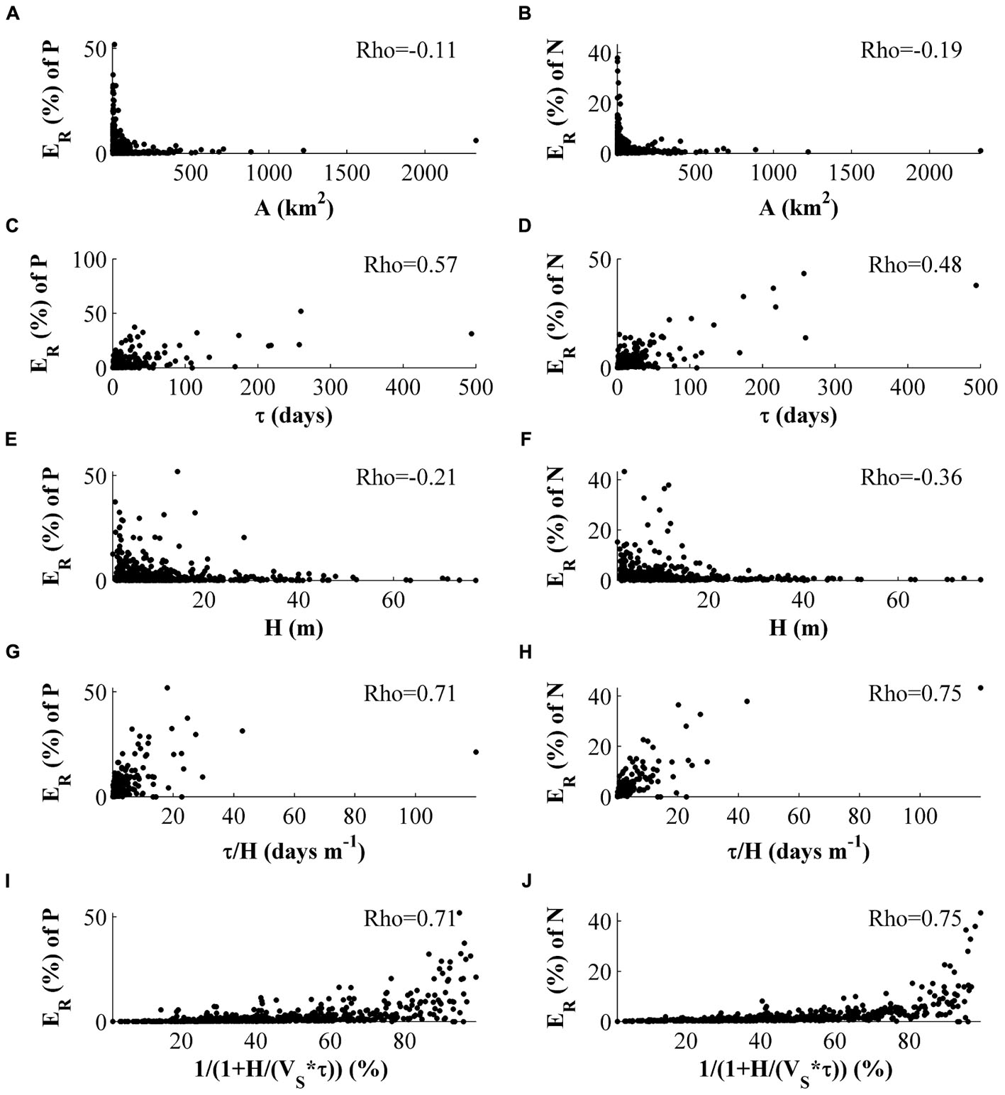
FIGURE 9. Association of E_R (PNR in percent of total load per area) with physical characteristics of the basins, i.e., surface area (A) (A,B), residence time (τ) (E,F) and mean depth (H) (C,D), in different formulations (G,H,I,J). V_S is set to 1. Only statistically significant (p < 0.05) Rho values are printed in the figure.

The apparent removal rate (V_S) seems to have similar associations with the environmental factors for both nutrients and will be evaluated together (Figure 10). Where important differences occur they will be mentioned. The averaged V_S for the Swedish coast was estimated to 0.025 m day^-1 for phosphorus and to 0.022 m day^-1 for nitrogen with ranges of 0–0.43 m day^-1 and 0–0.16 m day^-1 for phosphorus and nitrogen, respectively. For nitrogen, V_S tends to be higher on the West Coast while for phosphorus the highest average is calculated for the Bothnian Bay.

FIGURE 10

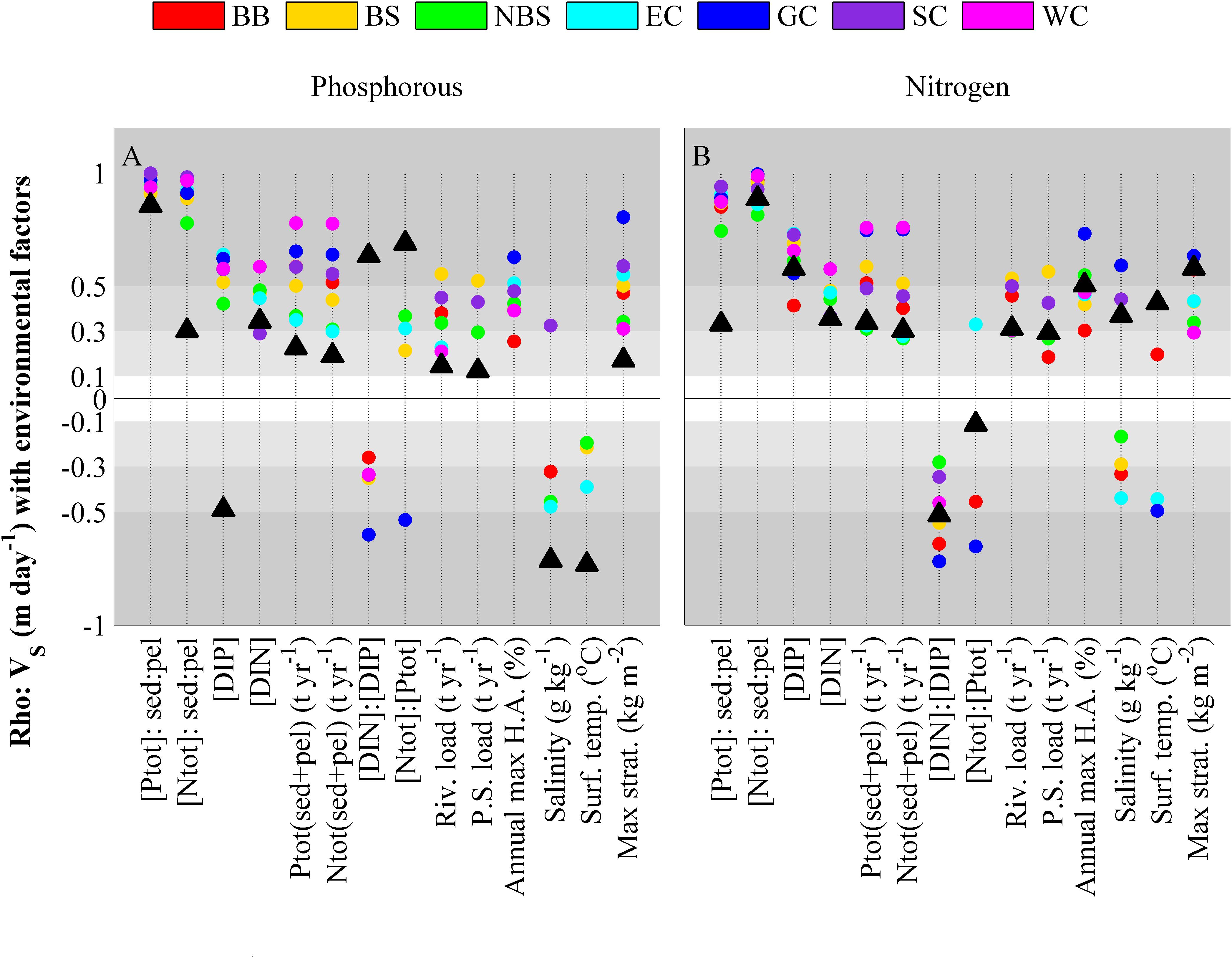
FIGURE 10. Spearmans rank correlation coefficients for the 20 years averaged V_S for phosphorous (A) and nitrogen (B) tested against environmental factors. All environmental factors are taken as 20-year averages from the model set-up, input or output. Concentrations are denoted with brackets and are expressed in mmol m^-3 for the water mass and mmol m^-2 for the sediment. DIN and DIP represents winter values (November–January). In the labels, hypoxic area has been abbreviated with H.A and point sources with P.S. Colored dots shows correlations within one of the MRs and black triangles denote the correlation of all water bodies along the Swedish coast. Insignificant correlations (p > 0.05) are not shown.

The theory in Section “Theory of Steady State Retention” for a steady state water body suggested that the M_sed:C_pel ratio would affect the retention efficiency and the results in Figures 10A,B affirm this assumption. The M_sed:C_pel ratio stands out as positively associated with retention efficiency for both nutrients in all MRs. The association is strong and homogeneous across the MRs. For the coast as a whole E_R of nitrogen is also strongly associated to the nitrogen M_sed:C_pel ratio and likewise E_R of phosphorus associates strongly to the phosphorus M_sed:C_pel ratio. However, for the coast as a whole the nutrient retention does not cross-associate.

V_S has a weaker, but homogeneous, positive association with stratification strength, the maximum hypoxic area and with all expressions of nutrient concentration. Thus, the permanent retention of both nitrogen and phosphorus generally tends to increase with eutrophication. For the entire coast (black triangles in Figure 10), V_S can be differently associated with some environmental indicators than what is seen for the MRs when they are evaluated separately. This is due to model settings and climate differences along the coast that affect some indices. This concerns DIP, DIN:DIP, pelagic Ntot:Ptot, surface temperature and salinity.

The only clearly negative association, i.e., indicated by a significant association in a majority of the evaluated regions and without contradictory results, in Figure 10 is the V_S of nitrogen that is negatively associated to the pelagic DIN:DIP factor in all MRs. Thus, the modeled retention of nitrogen is more effective at lower N:P ratios, i.e., when there is no overabundance of nitrogen. When looking into the details of the association (not shown), the same tendency is found for phosphorus V_S. For the remaining environmental indices the correlation is either insignificant or the association to retention efficiency seem to vary between the regions (the colored dots are scattered and/or of different sign).

The same analyze was performed for Blr, calculated from re-arrangement of Eq. (10) (not shown) but fewer clear associations were found. The analyze gave no clear indication of which environmental condition that are associated with high benthic loss rates of phosphorus but for nitrogen associations to M_sed:C_pel, both inorganic and total nutrient rations and high surface temperatures were found. The associations to nutrient ratios were positive in all MRs except for the Bothnian Bay coastline where the association was positive up to an N:P of about 50 but decreased after that point. For phosphorus an average Blr was calculated to be 4e-10 day^-1 and for nitrogen 1e-9 day^-1.

Discussion

Model Validation

Properties such as integrated internal nutrient losses and retention efficiency are easily extracted from a numerical model since all the biogeochemical transformation rates are calculated for each water body. Thus, a modeling approach gives a homogeneous and more complete data-set than observations. However, model results will always be dependent on the parameterizations that describe the biogeochemical processes and by definition a model will never cover everything that can occur in reality. Also the forcing and boundary conditions may be crucial for the results. The essential question is if it is good enough to answer the question at hand. Although, the validation shown in this paper indicates that the average skill of the model is acceptable, it also shows that for individual basins it can be poor. Thus, the results cannot be expected to be valid for every local situation, but still good enough to extract system understanding. Also the limitations associated with measurements, e.g., restrictions in time and location, as well as differences in vertical distribution at the different stations within a single basin make it difficult to evaluate the models’ quality. One area mentioned explicitly in the results is the Gotland coastline. Unfortunately not enough validation data were available for this area and hence, not a single water body could be validated. The model calculations for the Gotland coastline gave very high retention and generally extreme values, and since no validation is available these results should be treated with precaution.

Uncertainty of Biogeochemical Processes

It must also be noted that some biogeochemical processes are still missing in the model formulation. For example, the assimilation of nutrients by macrophytes and benthic microphytes is not explicitly described in SCM. In the model, these nutrient uptakes are partly compensated for by pelagic production and subsequent sedimentation. The difference between production that falls onto sediment and a production that takes place directly on illuminated seafloor is uncertain. Benthic microalgae do play an important role for total primary production capacity, e.g., in the northern Baltic Sea (Ask et al., 2016). According to Sundbäck et al. (2004) microphytobenthic (MPB) nitrogen assimilation often exceeds nitrogen removal by denitrification, partly because MPB activity suppresses denitrification and benthic production by MPB, and thus affects nutrient pathways in the sediment. Perennial macrofauna retains assimilated nutrients interannually and the uptake can be substantial. The effect on nutrient retention does, however, depend on the type of macroplants. To cause a permanent removal of nutrients macrofauna needs to produce refractory organic material, which can increase the removal by burial but plants might also outcompete bacteria for nitrogen and thus, decrease denitrification (McGlathery et al., 2007). Macroalgae that are advected with the water or are decomposed on an annual basis will affect retention only temporary.

In order to fully evaluate and understand the relative role of MPB and macro faunal production on the long-term retention of supplied nutrients, a module that takes into account the many effects of both macrophytes and benthic microphytes is needed. This model development and its evaluation were outside the scope and main focus of this study. Also, modeled sediment concentrations should ideally be evaluated against measurements. This work is ongoing, but sediment nutrient data are scarce, as shown by Hoefsloot (2017).

Nutrient Retention Along the Swedish Coastline

In this study, the Swedish coastal zone retains the largest amount of nitrogen per area on the west coast while the highest amount of phosphorus per area is retained along the Bothnian Sea shore (Figure 7). The filter and retention efficiencies on the West Coast are either comparable or lower than the rest of the Swedish coastal zone (Table 2), even though the West Coast has a slightly higher V_S. Thus, it can be concluded that the high total retention on the West Coast is not due to a more effective removal but rather to high nutrient load, likely the land loads (Figures 3C,D). Since the West Coast has low E_R for phosphorus, the high load does not result in an equally high retention of this nutrient.

In contrast, the high phosphorus retention along the Bothnian Sea (WD2) shore is not due to high loads but to a high PNR. This is further intensified by a positive temporal retention, i.e., the area both removes phosphorus effectively but has also a build-up of phosphorus in the SCMs water and sediment storage during the evaluated period. The high PNR is due to the models high burial rate constant in WD2.

The high R_tot in some areas close to land, e.g., the inner Stockholm archipelago, are likely due to a combination of high loads and high E_R in many enclosed near shore locations while the higher retention in basins bordering the open sea is due to the load supplied from the open Baltic Sea.

Both PNR and ΔM were found to be associated to the size of the water bodies. For PNR the cause is that the burial of matter depends on the amount of sediment area available, i.e., a larger water body can bury a larger amount of nutrients. The proximity to land, and thus to the natural and anthropogenic forced variability of the land load, is likely to be the reason behind the positive association of ΔM with the surface area of water bodies. The smaller water bodies close to land are likely to have larger fluctuations in their nutrient load and thus, their nutrient content tends to vary more over time.

The Stockholm Archipelago Key Site

The Stockholm archipelago is included both as part of WD3 and as a key site. The WD3 has more than 100% filtration efficiency, while the filter efficiency at the Stockholm key site is lower and comparable to the numbers presented in Almroth-Rosell et al. (2016). The higher filtration for the larger WD3 area is in line with Almroth-Rosell et al. (2016), who concluded that filtration efficiency increased with increasing area as long as it receives roughly the same load. This is the case in WD3, and especially the Stockholm archipelago, since most of the land load is received from the lake Mälaren outlet in the innermost parts of the archipelago.

Effects of Temporary Retention

Another result that was mentioned already in Almroth-Rosell et al. (2016) is that estimated retention values are sensitive to trends in nutrient storage during the period. Usually these fluctuations of the nutrient pool are one or two orders of magnitude less than the permanent retention, but occasionally (e.g., the open coastline in the south of the Bothnian Bay in Table 3) these trends in nutrient storage significantly affect the calculation of the nutrient filter efficiency. Hence, the effect of the build-up of, or release from, the nutrient pool in water and sediment needs to be considered whenever nutrient retention is estimated from data that are restricted in time, especially in water bodies or regions in the inner coastal zone. Evaluations based on a short timespan will only give a snapshot of information and thus, has restricted usability. This is especially important for phosphorus for which the temporal retention can be of the same order of magnitude as the permanent retention and thus, the momentary retention can vary greatly from the long term average.

Long term changes in the nutrient storage of the coastal zone are caused partly by changes in the nutrient load from land but it also depends on the influx of nutrients from the Baltic Sea. The nutrient levels of the open Baltic Sea are regulated by both land loads and internal nutrient release and loss due to fluctuating oxygen concentrations in deep waters. Hence, both anthropogenic factors, such as increased eutrophication and more recently, the mitigation of eutrophication, but also the natural hypoxic/anoxic periods of the Baltic Sea can affect long-term nutrient trends in the coastal zone.

Reversely, the open Baltic Sea is also impacted by changes in the coastal zone since alterations of the coastal nutrient filter impact the effective nutrient load that reach the Baltic Sea, which will also affect the Baltic Seas’ eutrophic state and hence, the oxygen conditions.

Estimating Coastal Retention Efficiency and Filter Efficiency

The geographical area of the coastal filter estimation in this study and in Asmala et al. (2017) overlaps, but differs in extent, and the methodology differ substantially, i.e., numerical biogeochemical modeling versus synthesis and extrapolation of measured data. However, these studies agree on several characteristics of the nutrient filter in coastal zone of the Baltic Sea.

Asmala et al. (2017) estimated that the coastal filter around the entire Baltic Sea removes 16% of the nitrogen and 53% of the phosphorus inputs from land. This may be compared to our estimate of the filter efficiency for the Swedish coastal zone of about 54 and 70% for nitrogen and phosphorus, respectively. The calculated filter efficiency from our study are higher, but agree with Asmala et al. (2017), as well as with Almroth-Rosell et al. (2016), in the sense that the coastal zone is a more efficient filter for phosphorus than for nitrogen and that the coastal filter has an important function in retaining and removing nutrients in the Baltic Sea. In Savchuk (2018), this high filter efficiency for phosphorus in the coastal zone is questioned when set in context of the overall nutrient budget of the Baltic Sea. However, the numbers derived for the entire Baltic Sea area by Asmala et al. (2017) is based on a limited set of data and more research is needed to connect the perspectives of the coastal zone and the Baltic Sea as a whole. The high filter efficiency in our study is derived for the Swedish coastline and more detailed studies are needed to extrapolate the results to other coastal areas in the Baltic Sea.

Both the results presented here and in Asmala et al. (2017) indicate that archipelagos and open coastlines tend to be more efficient nutrient filter than other coastal types, but both modeling and measured data also suggest that the spread in removal rates and filter efficiency is very large. In this study, the variation within each type is greater than the differences between the type averages and we suggest that the variation is most likely due to retention efficiency having a strong dependency on physical characteristics such as residence times and mean depth. These factors are not necessarily consistent within a coastal type. The physical characteristics give a rough estimation of the retention efficiency, but environmental factors, such as M_sed:C_pel:, can give a range of PNR values for water bodies that have similar H and τ. Even though the values in Figure 5 are taken from several different studies, from different coastal types and produced with different methods, there is a correlation between physical factors and nutrient retention.

The identical association strengths found between H/τ and Eq. (6) (Figures 9G–J) are due to the fact that Eq. 6 does not include anything new compared to τ/H as long as V_S is assumed constant. The same factors are combined differently resulting in another type of distribution, which is not taken into account when Spearman’s Rho is used instead.

The Impact From Environmental Conditions on Nutrient Retention Efficiency

To get an improved estimation of retention the environmental conditions also need to be taken into account. Theory for a steady state water body suggests that the ratio between the nutrient content in sediment and the concentrations in water could be used to estimate V_S and this study affirms that it is a good approach to estimate retention efficiency also for transient systems. Thus, Eq. 9 and 10 together offers a way to estimate E_R for any water body. The theory does, however, disregard the specification of the load. It gives the retention of the total load, i.e., both land and air load but also the exchange with other areas and the open sea, and does not clearly state the relation to filtering of land load, which is often of interest. However, Asmala et al. (2017) found denitrification rates to be positively associated to nitrate concentrations and sediment organic carbon (%), which suggested a dependence on similar factors as is suggested here, i.e., association of V_S to the M_sed:C_pel ratio.

The environmental factors evaluated in Figure 10 should also be assumed to interact, e.g., the strength of stratification will affect the likelihood of stagnant deep water and hence, also the likelihood of a basin experiencing hypoxia and anoxia. Also DIN and DIP levels can elevate the risk of low oxygen levels and are of course related to the amounts of total N and P. One should note that both the benthic loss rate and the apparent removal rate might be model dependent and the applicability to other data-sets is therefore not known. However, the average values listed in this work includes a variety of hydrological, climate and anthropogenic conditions, and thus, the values are not specific for any such environmental setting.

An expected result would be that the hypoxic fraction was a better indicator of retention potential than what is suggested by the results in Figure 10 and the analyze of Blr’s association with environmental indices. The expectation is based on an assumed relation between denitrification rates and hypoxic conditions and also release of phosphorus from the sediments at anoxia. However, even though these relations most likely affect retention to some extent, they seem to be overshadowed by the association of retention and retention efficiency with factor concerning all water bodies, i.e., physical dimensions, nutrient levels, nutrient ratios and temperatures. To investigate the effects from oxygen deficiencies the selection of water bodies needs to be aimed at that question specifically.

The seasonal variations in temperature are shown to be significantly associated to nitrogen retention caused by denitrification in Eilola et al. (2017). In the present study, the correlation is less pronounced since an annually averaged temperature is used (Figure 10). This could also be the case for other ambient parameters that have their largest variation on the annual time scale, e.g., seasonal oxygen deficiencies.

Conclusion

This modeling study gives an overview of nutrient retention for the entire Swedish coast and covers an array of coastal types in different climates and anthropogenic settings. The work also attempts to not only describe and quantify nutrient removal, but to relate it to some driving factors, i.e., to aid modeling of open coastal and shelf seas, such as the Baltic Sea. In a near shore context the parameterization of what happens to constituents in the fresh to saline continuum is of importance.

The main conclusions from this study are as follows:

• The Swedish coastal zone filters about 60% (approximately 53% for nitrogen and 69% for phosphorus) of the nutrients it received from land and air and thus, less than half of the input from land can be assumed to be exported from the coastal zone to the open sea.

• The northern and eastern Baltic Sea coasts, including the Stockholm archipelago, all retain more than 100% of the land and air load they receive. Thus, they also filter the Baltic Sea water.

• The nutrient removal is most efficient close to land.

• Nutrient retention cannot strictly be estimated only from the coastal type of the water body since the long term retention efficiency depends mainly on physical characteristics, i.e., mean depth and residence time, which vary independently of the coastal type.

• The inherent physical retention is modified by the ambient environmental state of the water body. Higher nutrient retention was found to be associated primarily with high M_sed:C_pel ratios. This ratio is in turn related to the ambient state of a water body, but it consists of factors that are feasible to measure, and thus offers opportunities to monitor changes in the retention efficiency of the coastal zone.

• On interannual timescales, the retention in a water body changes due to changes in its nutrient storage, i.e., the water body withholds or releases nutrients due to interannual variations and long term trends.

• The long-term retention efficiency can be well estimated from expressions derived from a steady state situation, even if the system shows a trend in it’s nutrient content. The area specific retention can also be reasonably well estimated from a simple expression based on physical properties.

• The most effective filtering of nutrients occurs in areas with low land load normalized to the area that receives them, e.g., the southern part of the Swedish East Coast.

Data Availability

The raw data supporting the conclusions of this manuscript will be made available by the authors, without undue reservation, to any qualified researcher.

Author Contributions

ME formulated the first draft of the concept for the study, performed the model run, and analyzed the model output. ME also wrote the main share of the manuscript. HM, KE, and EA-R contributed to the conception and design of the study and to the writing of the manuscript, adding important intellectual content. IW and LA contributed to the writing of the manuscript, also adding important intellectual content. All co-authors read and approved the submitted manuscript version.

Funding

The research presented in this study was part of the Baltic Earth Programme (Earth System Science for the Baltic Sea region, see http://www.baltex-research.eu/balticearth) and is part of the BONUS COCOA (Nutrient COcktails in COAstal zones of the Baltic Sea) project, which has received funding from BONUS, the Joint Baltic Sea Research and Development Programme (Art 185), funded jointly from the European Union’s Seventh Programme for research, technological development and demonstration and from the Swedish Research Council for Environment, Agricultural Sciences and Spatial Planning (FORMAS), grant no. 2013–2056. Additional financing has been received from the Swedish Agency for Marine and Water Management grant 1:12 Environmental management of marine and inland waters, tasks performed in accordance with regulation (204:660) regarding water quality considerations.

Conflict of Interest Statement

The authors declare that the research was conducted in the absence of any commercial or financial relationships that could be construed as a potential conflict of interest.

Footnotes

1. ^ https://www.bonusportal.org/projects/viable_ecosystem_2014-2018/cocoa
2. ^ http://viss.lansstyrelsen.se/
3. ^ http://www.smhi.se/klimatdata/oceanografi/havsmiljodata/marina-miljoovervakningsdata

References

Almroth-Rosell, E., Edman, M., Eilola, K., Meier, H. E. M., and Sahlberg, J. (2016). Modelling nutrient retention in the coastal zone of an eutrophic sea. Biogeosciences 13, 5753–5769. doi: 10.5194/bg-13-5753-2016

CrossRef Full Text | Google Scholar

Almroth-Rosell, E., Eilola, K., Hordoir, R., Meier, H. E. M., and Hall, P. O. J. (2011). Transport of fresh and resuspended particulate organic material in the Baltic Sea — a model study. J. Mar. Syst. 87, 1–12. doi: 10.1016/j.jmarsys.2011.02.005

CrossRef Full Text | Google Scholar

Almroth-Rosell, E., Eilola, K., Kuznetsov, I., Hall, P. O. J., and Meier, H. E. M. (2015). A new approach to model oxygen dependent benthic phosphate fluxes in the Baltic Sea. J. Mar. Syst. 144, 127–141. doi: 10.1016/j.jmarsys.2014.11.007

CrossRef Full Text | Google Scholar

Areskoug, H. (1993). Nedfall av Kväve och Fosfor till Sverige, Östersjön och Västerhavet. Report No. 4148. Solna: Swedish Environmental Protection Agency.

Ask, J., Rowe, O., Brugel, S., Strömgren, M., Byström, P., and Andersson, A. (2016). Importance of coastal primary production in the northern Baltic Sea. Ambio 45, 635–648. doi: 10.1007/s13280-016-0778-5

PubMed Abstract | CrossRef Full Text | Google Scholar

Asmala, E., Carstensen, J., Conley, D. J., Slomp, C. P., Stadmark, J., and Voss, M. (2017). Efficiency of the coastal filter: nitrogen and phosphorus removal in the Baltic Sea. Limnol. Oceanogr. 62, S222–S238. doi: 10.1002/lno.10644

CrossRef Full Text | Google Scholar

Billen, G., Silvestre, M., Grizzetti, B., Leip, A., Garnier, J., Voss, M., et al. (2011). “Nitrogen flows from European regional watersheds to coastal marine waters,” in European Nitrogen Assessment Sources, Effects and Policy Perspectives, eds M. A. Sutton, C. M. Howard, and J. W. Erisman (Cambridge: Cambridge University Press), 271–297. doi: 10.1017/CBO9780511976988.016

CrossRef Full Text | Google Scholar

Bolin, B., and Rodhe, H. (1973). A note on the concepts of age distribution and transit time in natural reservoirs. Tellus 25, 58–62. doi: 10.3402/tellusa.v25i1.9644

CrossRef Full Text | Google Scholar

Carstensen, J., Conley, D., Bonsdorff, E., Gustafsson, B., Hietanen, S., Janas, U., et al. (2014). Hypoxia in the Baltic Sea: biogeochemical cycles, benthic fauna, and management. AMBIO 43, 26–36. doi: 10.1007/s13280-013-0474-7

PubMed Abstract | CrossRef Full Text | Google Scholar

Conley, D., Bjorck, S., Bonsdorff, E., Carstensen, J., Destouni, G., and Gustafsson, B. (2009). Hypoxia-related processes in the Baltic Sea. Environ. Sci. Technol. 43, 3412–3420. doi: 10.1021/es802762a

PubMed Abstract | CrossRef Full Text | Google Scholar

Conley, D. J., Carstensen, J., Aigars, J., Axe, P., Bonsdorff, E., Eremina, T., et al. (2011). Hypoxia is increasing in the coastal zone of the Baltic Sea. Environ. Sci. Technol. 45, 6777–6783. doi: 10.1021/es201212r

PubMed Abstract | CrossRef Full Text | Google Scholar

Cossellu, M., and Nordberg, K. (2010). Recent environmental changes and filamentous algal mats in shallow bays on the Swedish west coast—A result of climate change? J. Sea Res. 63, 202–212. doi: 10.1016/j.seares.2010.01.004

CrossRef Full Text | Google Scholar

Edman, M., and Omstedt, A. (2013). Modeling the dissolved CO2 system in the redox environment of the Baltic Sea. Limnol. Oceanogr. 58, 74–92. doi: 10.4319/lo.2013.58.1.0074

CrossRef Full Text | Google Scholar

Edman, M. K., and Anderson, L. G. (2014). Effect on pCO 2 by phytoplankton uptake of dissolved organic nutrients in the central and Northern Baltic Sea, a model study. J. Mar. Syst. 139, 166–182. doi: 10.1016/j.jmarsys.2014.06.004

CrossRef Full Text | Google Scholar

Eilola, K., Gustafsson, B. G., Kuznetsov, I., Meier, H. E. M., Neumann, T., and Savchuk, O. P. (2011). Evaluation of biogeochemical cycles in an ensemble of three state-of-the-art numerical models of the Baltic Sea. J. Mar. Syst. 88, 267–284. doi: 10.1016/j.jmarsys.2011.05.004

CrossRef Full Text | Google Scholar

Eilola, K., Lindqvist, S., Almroth-Rosell, E., Edman, M., Wåhlström, I., Bartoli, M., et al. (2017). Linking Process Rates with Modelling Data and Ecosystem Characteristics. Report Oceanography No. 61. Norrköping: Swedish Meteorological and Hydrological Institute.

Google Scholar

Eilola, K., Meier, M. H. E., and Almroth, E. (2009). On the dynamics of oxygen, phosphorus and cyanobacteria in the Baltic Sea; a model study. J. Mar. Syst. 75, 163–184. doi: 10.1016/j.jmarsys.2008.08.009

CrossRef Full Text | Google Scholar

Engqvist, A., Döös, K., and Andrejev, O. (2006). Modeling water exchange and contaminant transport through a Baltic coastal region. AMBIO 35, 435–447. doi: 10.1579/0044-7447(2006)35[435:MWEACT]2.0.CO;2

PubMed Abstract | CrossRef Full Text | Google Scholar

European Parliament Council of the European Union. (2000). Directive 2000/60/EC of the European Parliament and of the Council of 23 October 2000 Establishing a Framework for Community Action in the Field of Water Policy. Available at: http://data.europa.eu/Eli/dire/2000/60/O: Official Journal of the European Communities L 327

Google Scholar

Fonselius, S., and Valderrama, J. (2003). One hundred years of hydrographic measurements in the Baltic Sea. J. Sea Res. 49, 229–241. doi: 10.1016/S1385-1101(03)00035-2

CrossRef Full Text | Google Scholar

Gräwe, U., Naumann, M., Mohrholz, V., and Burchard, H. (2015). Anatomizing one of the largest saltwater inflows into the Baltic Sea in December 2014. J. Geophys. Res. 120, 7676–7697. doi: 10.1002/2015JC011269

CrossRef Full Text | Google Scholar

Gustafsson, B., Schenk, F., Blenckner, T., Eilola, K., Meier, H. E. M., Müller-Karulis, B., et al. (2012). Reconstructing the development of Baltic Sea Eutrophication 1850–2006. AMBIO 41, 534–548. doi: 10.1007/s13280-012-0318-x

PubMed Abstract | CrossRef Full Text | Google Scholar

Hāggmark, L., Ivarsson, K. I., Gollvik, S., and Olofsson, P. O. (2000). Mesan, an operational mesoscale analysis system. Tellus A 52, 2–20. doi: 10.3402/tellusa.v52i1.12250

CrossRef Full Text | Google Scholar

Hayn, M., Howarth, R., Marino, R., Ganju, N., Berg, P., Foreman, K. H., et al. (2014). Exchange of nitrogen and phosphorus between a shallow lagoon and coastal waters. Estuaries Coast. 37, 63–73. doi: 10.1007/s12237-013-9699-8

PubMed Abstract | CrossRef Full Text | Google Scholar

Helcom. (2017). First Version of the ‘State of the Baltic Sea’ Report – June 2017 – to be Updated in 2018. Avaliable at: http://stateofthebalticsea.helcom.fi

Hoefsloot, I. (2017). Validation of Modelled Benthic Nutrients in the Swedish Coastal Zone Model and the Effects of Microphytobenthos Implementation. Utrecht: Utrecht University.

Leppäranta, M., and Myrberg, K. (2009). Physical Oceanography of the Baltic Sea. Berlin: Springer Science & Business Media. doi: 10.1007/978-3-540-79703-6

CrossRef Full Text | Google Scholar

Lilliefors, H. W. (1967). On the kolmogorov-smirnov test for normality with mean and variance unknown. J. Am. Stat. Assoc. 62, 399–402. doi: 10.1080/01621459.1967.10482916

CrossRef Full Text | Google Scholar

Lindstrom, G., Pers, C., Rosberg, J., Stromqvist, J., and Arheimer, B. (2010). Development and testing of the HYPE (Hydrological Predictions for the Environment) water quality model for different spatial scales. Hydrol. Res. 41, 295–319. doi: 10.2166/nh.2010.007

CrossRef Full Text | Google Scholar

Marmefelt, E., Arheimer, B., and Langner, J. (1999). An integrated biochemical model system for the Baltic Sea. Hydrobiologia 393, 45–56. doi: 10.1023/A:1003541816177

PubMed Abstract | CrossRef Full Text | Google Scholar

McGlathery, K. J., Sundbäck, K., and Anderson, I. C. (2007). Eutrophication in shallow coastal bays and lagoons: the role of plants in the coastal filter. Mar. Ecol. Prog. Ser. 348, 1–18. doi: 10.3354/meps07132

CrossRef Full Text | Google Scholar

Meier, H., and Kauker, F. (2003). Modeling decadal variability of the Baltic Sea: 2. Role of freshwater inflow and large-scale atmospheric circulation for salinity. J. Geophys. Res. 108:3368. doi: 10.1029/2003JC001799

CrossRef Full Text | Google Scholar

Meier, M., Eilola, K., and Almroth, E. (2011). Climate-related changes in marine ecosystems simulated with a 3-dimensional coupled physical-biogeochemical model of the Baltic Sea. Clim. Res. 48, 31–55. doi: 10.3354/cr00968

CrossRef Full Text | Google Scholar

Neumann, T., Fennel, W., and Kremp, C. (2002). Experimental simulations with an ecosystem model of the Baltic Sea: a nutrient load reduction experiment. Global Biogeochem. Cycles 16:1033. doi: 10.1029/2001GB001450

CrossRef Full Text | Google Scholar

Nixon, S. W., Ammerman, J. W., Atkinson, L. P., Berounsky, V. M., Billen, G., Boicourt, W. C., et al. (1996). “The fate of nitrogen and phosphorus at the land-sea margin of the North Atlantic Ocean,” in Nitrogen Cycling in the North Atlantic Ocean and its Watersheds, ed. R. Howarth (Berlin: Springer), 141–180. doi: 10.1007/978-94-009-1776-7_4

CrossRef Full Text | Google Scholar

Norkko, A., and Bonsdorff, E. (1996). Rapid zoobenthic community responses to accumulations of drifting algae. Mar. Ecol. Prog. Ser. 131, 143–157. doi: 10.3354/meps131143

CrossRef Full Text | Google Scholar

Oschlies, A., Blackford, J., Doney, S. C., and Gehlen, M. (2010). “Modelling considerations,” in Guide to Best Practices for Ocean Acidification Research and Data Reporting, eds U. Riebesell, V. J. Fabry, L. Hansson, and J.-P. Gattuso (Luxembourg City: Publications Office of the European Union), 233–242.

Google Scholar

Robertson, L., Langner, J., and Engardt, M. (1999). An Eulerian limited-area atmospheric transport model. J. Appl. Meteorol. 38, 190–210. doi: 10.1175/1520-0450(1999)038<0190:AELAAT>2.0.CO;2

CrossRef Full Text | Google Scholar

Rönnberg, C., and Bonsdorff, E. (2004). Baltic Sea eutrophication: area-specific ecological consequences. Hydrobiologia 514, 227–241. doi: 10.1023/B:HYDR.0000019238.84989.7f

CrossRef Full Text | Google Scholar

Savchuk, O. P. (2018). Large-scale nutrient dynamics in the Baltic Sea, 1970–2016. Front. Mar. Sci. 5:95. doi: 10.3389/fmars.2018.00095

CrossRef Full Text | Google Scholar

Seifert, T., and Kayser, B. (1995). A High Resolution Spherical Grid Topography of the Baltic Sea. Rostock: Institut fur Ostseeforschung.

Google Scholar

Sheldon, J. E., and Alber, M. (2006). The calculation of estuarine turnover times using freshwater fraction and tidal prism models: a critical evaluation. Estuaries Coasts 29, 133–146. doi: 10.1007/bf02784705

CrossRef Full Text | Google Scholar

Sundbäck, K., Linares, F., Larson, F., Wulff, A., and Engelsen, A. (2004). Benthic nitrogen fluxes along a depth gradient in a microtidal fjord: the role of denitrification and microphytobenthos. Limnol. Oceanogr. 49, 1095–1107. doi: 10.4319/lo.2004.49.4.1095

CrossRef Full Text | Google Scholar

Svensson, U. (1998). PROBE program for boundary layers in the environment system description and manual. SMHI Rep. Oceanogr. 24:42.

Google Scholar

Wulff, F., and Stigebrandt, A. (1989). A time-dependent budget model for nutrients in the Baltic Sea. Global Biogeochem. Cycles 3, 63–78. doi: 10.1029/GB003i001p00063

CrossRef Full Text | Google Scholar