 Lisa Fiedler
 Martin Middendorf
 Matthias Bernt
- 1Department of Computer Science, Leipzig University, Leipzig, Germany
- 2Helmholtz Centre for Environmental Research—UFZ, Leipzig, Germany
A wide range of scientific fields, such as forensics, anthropology, medicine, and molecular evolution, benefits from the analysis of mitogenomic data. With the development of new sequencing technologies, the amount of mitochondrial sequence data to be analyzed has increased exponentially over the last few years. The accurate annotation of mitochondrial DNA is a prerequisite for any mitogenomic comparative analysis. To sustain with the growth of the available mitochondrial sequence data, highly efficient automatic computational methods are, hence, needed. Automatic annotation methods are typically based on databases that contain information about already annotated (and often pre-curated) mitogenomes of different species. However, the existing approaches have several shortcomings: 1) they do not scale well with the size of the database; 2) they do not allow for a fast (and easy) update of the database; and 3) they can only be applied to a relatively small taxonomic subset of all species. Here, we present a novel approach that does not have any of these aforementioned shortcomings, (1), (2), and (3). The reference database of mitogenomes is represented as a richly annotated de Bruijn graph. To generate gene predictions for a new user-supplied mitogenome, the method utilizes a clustering routine that uses the mapping information of the provided sequence to this graph. The method is implemented in a software package called DeGeCI (De Bruijn graph Gene Cluster Identification). For a large set of mitogenomes, for which expert-curated annotations are available, DeGeCI generates gene predictions of high conformity. In a comparative evaluation with MITOS2, a state-of-the-art annotation tool for mitochondrial genomes, DeGeCI shows better database scalability while still matching MITOS2 in terms of result quality and providing a fully automated means to update the underlying database. Moreover, unlike MITOS2, DeGeCI can be run in parallel on several processors to make use of modern multi-processor systems.
1 Introduction
Mitochondria are spherical organelles found in most eukaryotic cells. Their genome, the mitogenome, differs in various aspects from their nuclear counterpart, which include their size, structure, and composition. In Metazoa, the mitogenome is commonly organized as a double-stranded circular DNA molecule with an average length of approximately 16, 500 nt and a small core set of 37 genes, comprised of 13 protein-coding genes, 22 tRNAs, two rRNAs, and one non-coding region, which contains most of the regulatory elements (Wolstenholme, 1992). Although the gene content is generally well conserved, the gene arrangement varies greatly among animal mitogenomes. This renders them an attractive target for a variety of comparative analyses, such as phylogenetic reconstruction or genome rearrangement studies. To facilitate such analyses to be performed systematically on a large scale, automated, standardized annotation of the mitogenome is an indispensable prerequisite.
The widest selection of publicly available mitochondrial genome data can be found in the GenBank (Benson et al., 2000) and RefSeq (Pruitt et al., 2007) databases. GenBank offers access to original sequence data, whereas RefSeq provides a non-redundant expert-curated collection of original GenBank entries. Several databases and tool sets have been built on these data repositories to generate (de novo) annotations for user-supplied sequence data, e.g., DOGMA (Wyman et al., 2004), MOSAS (Sheffield et al., 2010), MitoFish (Iwasaki et al., 2013), and MITOS (Bernt et al., 2013). These approaches identify genes using either the sequence similarity search against sequence databases, containing gene sequences of published mitogenomes, or search with curated (hidden Markov/covariance) gene models. All the aforementioned approaches identify protein-coding genes using BLASTX and/or BLASTN searches against an internal database. DOGMA, MOSAS, and MitoFish further apply this technique to rRNA gene detection, whereas MITOS uses Infernal (Eddy, 2002; Nawrocki et al., 2009) and covariance models for mitochondrial rRNAs to serve this purpose. For tRNA annotation, MITOS uses covariance models (Eddy and Durbin, 1994), DOGMA employs COVE, MOSAS applies ARWEN and tRNAscan-SE (Lowe and Eddy, 1997), and MitoFish makes use of MiTFi. Meanwhile, an updated and improved version, MITOS2, was developed, which is based on a more current RefSeq release and allows us to search for protein-coding genes with profile hidden Markov models (HMMs) (Donath et al., 2019). One drawback of DOGMA and MOSAS is that they require some manual improvements on the result set. MOSAS’s restriction to insects and MitoFish’s restriction to fishes limit their scope of application. The fast-growing amount of available mitogenomes creates two problems for all of the aforementioned approaches: 1) the runtime for the sequence similarity search increases approximately linearly with the database size and 2) the necessary curation of gene models impedes automatic updates that allow the inclusion of new sequence data that becomes available over time.
de Bruijn graphs (Bruijn, 1946; Good, 1946) are an important data structure for compact sequence data representation. To this end, sequences are decomposed into small segments, the so-called k-mers, which form the vertices of this graph. Two vertices are connected if the suffix of length k − 1 of the first vertex is equal to the prefix of length k − 1 of the second vertex. In the field of bioinformatics, de Bruijn graphs have often been used for DNA fragment assembly, such as in Pevzner et al. (2001), Pevzner et al. (2004), and Zerbino and Birney (2008). The latter employs a modified de Bruijn graph, the A-Bruijn graph, which can also be used for repeat classifications. Another variant is the manifold de Bruijn graph (Lin and Pevzner, 2014), which allows using (k + 1)-mers of variable lengths, choosing larger values for high-coverage regions and smaller values for low-coverage regions. However, the focus of these applications has been on nuclear genomes. Their huge sequence length, as opposed to mitochondrial genomes, explains the emergence of vastly compressed storage structures proposed in the literature to keep the required amount of memory as small as possible. One such structure is introduced by Bowe et al. (2012). Almodaresi et al. (2017) extended this approach by additionally allowing us to store a single property, the “color,” per edge. For many applications, such as variant detection, the approach is sufficient where keeping track of the identity of each of the contributing sequences is the only focus. However, if several properties need to be considered, this storage structure cannot be used. Another downside, which also applies to A-Bruijn and manifold de Bruijn graphs, is that they are all generated based on a fixed set of input genomes. When additional sequences need to be embedded or some contained sequences need to be removed, the entire graph must be reconstructed, which is already, for a moderate amount of genomes and/or long sequence lengths, a time-consuming task.
This work presents DeGeCI (De Bruijn graph Gene Cluster Identification), a new method for the efficient automatic gene detection of mitochondrial genomes. This method uses a collection of mitogenomes, whose sequence data are represented as a richly annotated Mitochondrial De Bruijn Graph (MDBG). To annotate an input sequence rin, a subgraph
2 Methods
2.1 Graph structure
Given a string (i.e., a sequence of characters), a k-mer is a substring of length k. A string can be disassembled into all of its (k + 1)-mers by sliding a window of length (k + 1) over the string while retaining duplicates. A genome r is a string composed of nucleotides A, C, T, and G, where circular genomes are linearized by “cutting” the genome at an arbitrary but fixed location.
In the proposed de Bruijn graph, MDBG (V, E), over a set of genomes G with the vertex set V and edge set E, each (k + 1)-mer x1x2 … xk+1 of every genome in G leads to two vertices v and v′ in V, representing the k-prefix x1x2 … xk and k-suffix x2 … xk+1, respectively. These are connected by directed edges (v and v′), which represent the (k + 1)-mer itself. For circular genomes, the (k + 1)-mers that connect both sides of the linearized string representation are also included. Thus, while each linear genome of length |r| contributes |r| − k many (k + 1)-mers, a circular genome of this length contributes |r| many (k + 1)-mers to the graph. The complementary DNA strand (negative strand), with an opposite reading direction, is taken into account by adding the reverse complement of each (k + 1)-mer to MDBG. Each edge (v and v′) is annotated with a label r, denoting the genome from which this edge originates, the strandedness σ ∈ { +, − }, and the position p (with respect to the positive strand) of nucleotide xk+1 of (v and v′) in genome r. This allows for an unambiguous reconstruction of each genome in G from MDBG (V, E). It should be noted that each (k + 1)-mer that is contained in multiple different genomes or is contained multiple times in the same genome (i.e., due to repeats) results in a pair of vertices that is connected by multiple edges, the so-called parallel edges. The MDBG is thus a multigraph. Figure 1 illustrates an example of the de Bruijn graph of a circular genome r with the sequence ACTGAA for k = 3 on the positive strand.
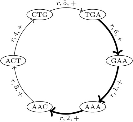
FIGURE 1. de Bruijn graph of a circular genome r with the sequence ACTGAA for k = 3 and positive strand σ = +. The SGT (3, 2, r, +) is exemplarily shown. The corresponding edges in the graph are highlighted in bold.
A trail in a graph is a sequence of distinct edges that joins a sequence of vertices. Let (i, j, r, σ) be the trails in MDBG, denoting a single genome trail (SGT), which is composed of edges corresponding to the subsequence from the position i to j in the genome r located on the strand σ. For a circular genome, i >j, if the associated subsequence extends over the string boundary of the linearized genome representation. In the de Bruijn graph depicted in Figure 1, one such SGT is exemplarily highlighted.
2.2 Workflow
For the de novo annotation of an input genome rin, DeGeCI requires only its nucleotide sequence. The DeGeCI pipeline consists of six major stages, which are summarized in Figure 2. The following sections present the individual steps involved.
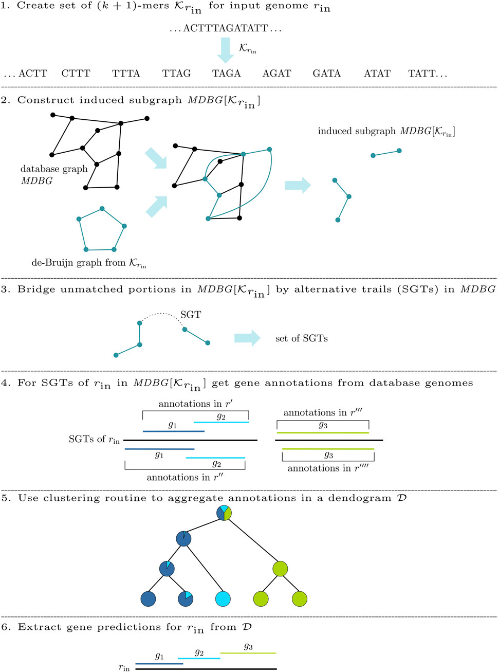
FIGURE 2. DeGeCI workflow for the de novo annotation of an input genome rin.
2.2.1 Subgraph construction
Initially, DeGeCI generates the set
2.2.2 Connected component bridging
Even if dense taxon sampling is provided in the database graph, input species with a poorly conserved gene content can lead to (k + 1)-mers in
While two CCs of
To identify such connecting trails, an algorithm called cc-bridging was developed. The pseudocode is given in Algorithm 1. For each CC CI, induced by subsequence sI, bridging is initially attempted with CC CT, induced by subsequence sT, which among all inducing subsequences of CCs in
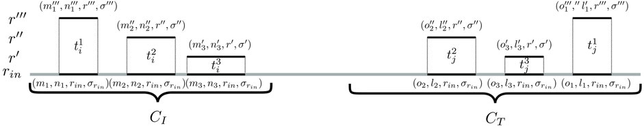
FIGURE 3. Identification of bridging trails for components CI and CT. In this example, there are three pairs of seeding SGTs
Algorithm 1. CC-BRIDGING.

2.2.2.1 Validation of seeding trails
The validation of the seeding trails for two CCs, CI and CT (line 16 in Algorithm 1), consists of the following two steps:
Step 1:. Identification of bridging candidates. The method searches for seeding SGTs (m′, n′, r, σ) ∈ CI and (o′, l′, r, σ) ∈ CT so that there are mapping input genome SGTs
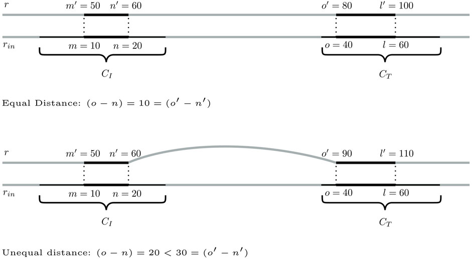
FIGURE 4. Two scenarios for a pair of seeding SGTs of database genome r in CCs CI and CT, for which a distance of
Step 2:. Pairwise sequence alignments. For each of the remaining SGT pairs, the corresponding bridging trails are examined for sequence similarity to the input genome. To this end, the algorithm conducts local pairwise sequence alignments with affine gap costs (cf. Supplementary Material: Section 5 for details) between the unmapped input sequence segment and sequences that correspond to the bridging trails. Alignments are accepted if they have an E-value of at most 10–3.
2.2.3 Gene annotation
The basis for the annotation of the input genome rin is a collection of gene annotations
For each pair of mapping SGTs
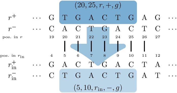
FIGURE 5. Input genome SGT
An annotation in
It is to be expected that flawed annotations in
2.2.3.1 Aggregating gene predictions
The pseudocode of clusterG is given in Algorithm 2. The algorithm is performed individually with gene predictions
Algorithm 2. CLUSTERG.
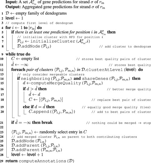
Initially, every position i of rin constitutes a cluster
where
is considered. Here, χP equals one if predicate P is true and zero otherwise, setting the probability of a gene to zero if it does not appear in both contributing distributions. This is to prevent the annotation of a gene at positions that are not predicted by any of the genomes in the database.Given such a joined RFD of n genes, the smallest number t ≤n of genes necessary to obtain a cumulated relative frequency of at least 0.95 is identified. Merged clusters with a low value of t feature a joined RFD where much weight falls on few genes. This indicates that the two entering clusters can be combined to a consistent prediction, assigning a higher quality to the merge.At some point, there will most likely be more than one pair of clusters with the smallest value of t among all mergeable clusters. In such a case, clusters with a higher maximum score
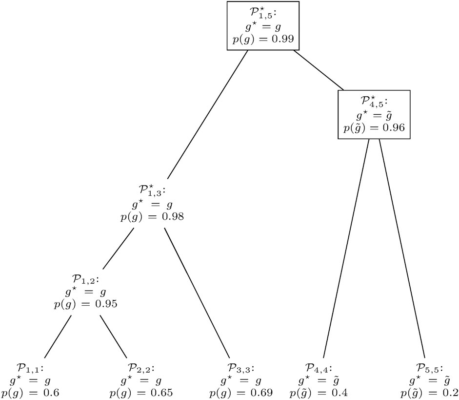
FIGURE 6. Gene prediction retrieval from the clusters in
2.2.3.2 Handling unannotated regions
We recall that in the initial RFD Eq. 1, each prediction of gene g is scaled with weight ωg, which is the reciprocal of the length of such a gene on average. However, there is no reasonable definition of such a length for unannotated regions, i.e., where g = g0. Thus, prior to clustering, positions p of rin, presumably not encoding any actual gene, are identified as follows: there are more predictions with g = g0 than with the total number of predictions of the two (or one if there is only one) best scoring genes g ≠ g0 at p or the cumulative relative frequency of these genes falls below 0.8. The rationale behind taking the two best scoring genes into account is that two genes may well overlap, but the precise gene boundaries may vary slightly among different genomes.
2.3 Implementation
DeGeCI is available as a free open-source software package1. It is implemented in Apache Spark (Veith and de Assuncao, 2019) using its Java API, facilitating parallel program execution. The database graph MDBG is stored in an indexed PostgreSQL database (Stonebraker, 1987). PostgreSQL dump files for the database population are available for RefSeq 89 and RefSeq 2042.
To initiate the annotation of an input genome, its nucleotide sequence can be provided either as a FASTA file or as a sequence string. The final gene annotation is provided as a bed file.
3 Materials
To create the database graph MDBG, a comprehensive set of all 8,015 metazoan mitogenomes contained in RefSeq 89 was used. The k-mer size was set to k = 16, following a careful empirical analysis presented in Section 4.2.1. The curated GenBank files of the RefSeq dataset served as a basis for the gene annotation of SGT mappings. To achieve a consistent nomenclature among all entries, an important prerequisite to derive joint annotation, each GenBank entry was parsed following the guidelines suggested by Boore (2006). The details are compiled in Supplementary Material: Section 2.
To assess the quality of the proposed method, DeGeCI was applied to a sample of 100 genomes of RefSeq 89 (for a complete list, see Supplementary Material: Section 6), for which expert-curated annotations exist. These annotations served as ground truth data, allowing us to assess the accuracy of the produced gene predictions. This sample was drawn by randomly selecting different numbers of genomes from each of the major metazoan groups contained in this RefSeq release. The number of species per group was chosen with respect to the frequency in which they occurred in RefSeq 89 (and, therefore, MDBG). This comprises seven Spiralia, 27 Arthropoda, 32 Actinopterygii, four Amphibia, 15 Mammalia, 13 Sauropsida, and two non-bilaterian species. In order to not to bias the gene predictions of an input genome of the sample with its annotation in the database graph, all edges of this genome in the database graph were excluded during the subgraph construction step of DeGeCI.
4 Results
This contribution presents a new de Bruijn graph-based method, DeGeCI, for de novo gene annotations of mitochondrial genomes. In the following, we compare DeGeCI with MITOS2 (Bernt et al., 2013), a widely used state-of-the-art annotation tool for mitochondrial genomes. Both MITOS2 and DeGeCI are based on an internal database of mitogenomic sequences of the RefSeq database and require only nucleotide sequences as input, allowing for a fair comparison.
While both tools are based on an internal database of mitogenomic sequences, the underlying approaches are essentially different. MITOS2 uses profile hidden Markov models in combination with methods from Donath et al. (2019) and the HMMER software suite (Eddy, 2011) or BLASTX searches (Altschul et al., 1990) for the annotation of protein-coding genes. To detect non-coding RNAs, i.e., tRNAs and rRNAs, MITOS2 uses Infernal (Eddy, 2002; Nawrocki et al., 2009) in the glocal search mode and curated covariance models. Contrarily, DeGeCI is a stand-alone application that relies on no third-party bioinformatics software. Both proteins and RNAs are annotated using the mapping information of the input genome to a database graph, in combination with a subsequent clustering approach.
4.1 Benchmarking procedure
To allow for a comparative evaluation with MITOS2, the following definitions are adopted from Bernt et al. (2013). For each DeGeCI/MITOS2 prediction, the corresponding RefSeq prediction is the annotation that has the largest position overlap with the DeGeCI/MITOS2 prediction, given that at least 75% of the DeGeCI/MITOS2 positions are shared with the RefSeq predictions. Each such allocation of a DeGeCI/MITOS2 annotation to a RefSeq annotation is classified as equal if both predict the same gene on the same strand, classified as different if both predict different genes, and classified as having a strand difference if both predict the same gene but on opposing strands. DeGeCI/MITOS2 predictions, where no corresponding RefSeq prediction is found, are classified as false positives (FPs). Analogously, RefSeq predictions without corresponding DeGeCI/MITOS2 predictions are classified as false negatives (FNs).
4.2 Parameter settings
For MITOS2, the default parameter setting and appropriate genetic codes were used for each of the 100 considered species. The parameters for DeGeCI were set as follows.
4.2.1 (k + 1)-mer size
To determine a suitable value for the (k + 1)-mer size of the database graph, the right balance has to be found between a too-small value, leading to a great number of random (k + 1)-mer matches, and a too-large value, concealing many sequence similarities among the genomes.
To this end, the following experiment was conducted 100 times for every
Figure 7 depicts these ratios for all
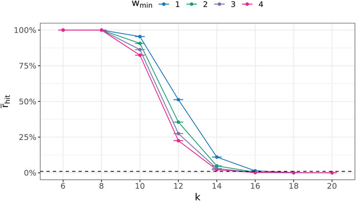
FIGURE 7. Average fraction
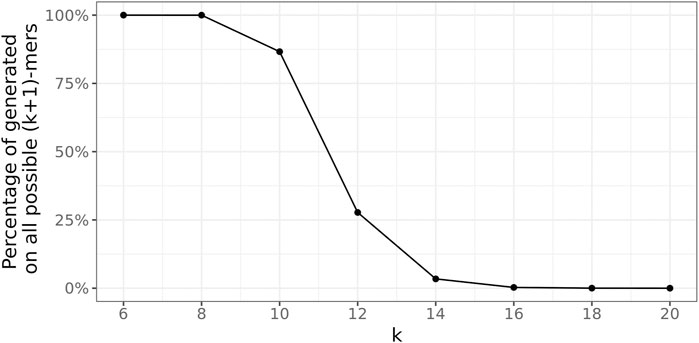
FIGURE 8. Percentage of unique true (k + 1)-mers on all possible 4k+1 unique (k + 1)-mers.
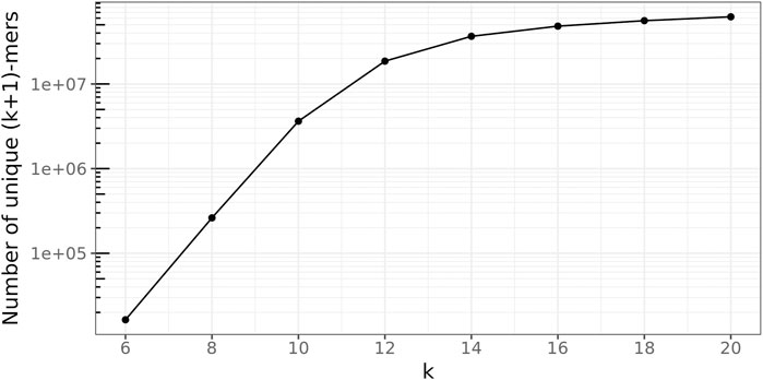
FIGURE 9. Number of unique true (k + 1)-mers on the log scale.
4.2.2 Sequence alignments
For sequence alignments, we applied match costs of 1, mismatch costs of −2, and gap penalties of −2 for opening and extending a gap. The E-value threshold was set at 10–3. These are common settings, which assume 95% of sequence conservation.
4.3 Comparison with MITOS2
Table 1 summarizes the annotation quality of DeGeCI and MITOS2 for all predictions together and also for the different groups of genes: proteins, tRNAs, and rRNAs. RefSeq 89 was used as a reference database for both tools. DeGeCI identified all of the rRNA and protein and 99% of tRNA RefSeq predictions with an equal gene and strand annotation. Thus, DeGeCI obtains an even larger number of correct predictions than MITOS2 (only 99.1% of the protein and 98.7% of the tRNA RefSeq predictions). A genewise and taxonomic breakdown of the results of both tools is compiled in Supplementary Material: Supplementary Tables S1–S11.
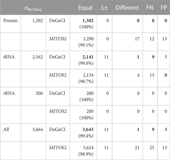
TABLE 1. Comparison of DeGeCI and MITOS2 predictions with RefSeq 89 annotations. Here, the number of RefSeq predictions
The main cause for the few RefSeq tRNA predictions without equal DeGeCI predictions is the annotation of opposing strands, i.e., corresponding RefSeq and DeGeCI predictions, which are classified as having a strand difference. This affects 11 predictions (see Supplementary Material: Supplementary Table S12 for details). In each such case, more than 95% of DeGeCI positions are shared with RefSeq positions, suggesting a high agreement of both predictions. DeGeCI also always annotates the negative strand, whereas RefSeq annotates the positive strand. Since a special “complement” tag needs to be set for a RefSeq annotation to indicate that the gene is located on the negative strand, there is a reason to presume that this tag was simply forgotten in the corresponding RefSeq entries. The fact that all 11 predictions were also annotated with the opposite strand by MITOS2 supports this hypothesis. Furthermore, nine of the RefSeq predictions stem from the same genome, and not a single gene of this genome is marked with the complement tag, indicating a systematic error in these RefSeq annotations.
There is one DeGeCI prediction that annotates a different gene rather than the corresponding RefSeq prediction, i.e., which has the classification as “different.” It involves the annotation of a different anticodon type of a leucine tRNA. As discussed in Bernt et al. (2013), there are inconsistencies in the naming scheme of RefSeq annotations, resulting in misannotations of the anticodon types of serine and leucine tRNAs (also cf. Supplementary Material: Section 2). Again, MITOS2 identifies the same discrepancy, leaving little doubt that the anticodon type of the RefSeq prediction should be different (cf. Supplementary Material: Supplementary Table S13).
The remaining nine RefSeq predictions without the corresponding equal DeGeCI prediction are FNs (25 in MITOS2), accounting for only 0.2% of the RefSeq entries (
There are very few (three) DeGeCI annotations that are classified as FPs, all of which are tRNAs. MITOS2, on the other hand, predicts 13 FPs, which are all proteins. For a complete list of FNs of both tools, see Supplementary Material: Supplementary Tables S14, S15 and for their FPs, see Supplementary Table S16.
4.4 Accuracy of gene predictions
The majority of the DeGeCI predictions are in much better agreement with the RefSeq predictions than the threshold of 75% overlap requires (cf. Supplementary Material: Supplementary Table S17). More precisely, the average fractions of the DeGeCI positions that are shared with those predicted by RefSeq exceed 98.7%, and the average fractions of RefSeq positions that are shared with those predicted by DeGeCI exceed 97.3% for all types of genes (similar for MITOS2).
DeGeCI also predicts start and end positions with fairly high precision. Table 2 shows that in 96% of the tRNA, 85% of the protein, and 78% of rRNA predictions, the start and stop positions vary by less than 5 nt from the RefSeq annotations. As can be seen from the table, 8% more of DeGeCI′s rRNA predictions were generated with this precision. For proteins and tRNAs, slightly more of the MITOS2 position predictions have a maximum deviation of 5 nt (5% and 3%). One has to keep in mind, however, that MITOS2 also produced more FP and FN predictions for both of these categories (see Table 1). Moreover, for proteins, a possible explanation for this discrepancy could be as follows: after producing protein position predictions, MITOS2 searches the proximity of every start and end position for start and stop codons, respectively. If valid start or stop codons are found, the gene boundary predictions are adapted accordingly. While this approach presumably improves the accuracy of the protein boundary predictions, there are several lineage-specific variations in the standard genetic code for mitogenomes. Thus, to detect appropriate start and end codons for the input genome, the adequate genetic code table must be specified by the user. Since DeGeCI tries to minimize the required amount of knowledge about the input genome and/or user expertise, this is currently not implemented in the DeGeCI pipeline. However, we would like to point out that such an extension would be possible. As soon as slightly larger deviations are considered (i.e., Δ nt ≥10), DeGeCI again produces more protein predictions than MITOS2 (see bold entries in Table 2).
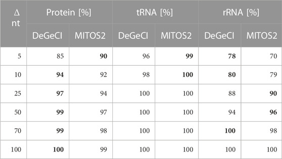
TABLE 2. Percentages of corresponding DeGeCI/MITOS2 and RefSeq predictions with start and stop positions of less than Δ nt. The higher rates are highlighted in bold.
4.5 RefSeq 204 as a reference database
We also validated DeGeCI′s performance using the more recent RefSeq release RefSeq 204, which contains 9,877 species, for the database graph. Using this larger database, two previous FNs and one FP could be eliminated in the sample set. None of the remaining predictions was impaired (for details, see Supplementary Material: Supplementary Table S18). Since MITOS2 currently only offers prepared databases for RefSeq 39, RefSeq 63, and RefSeq 89, a comparative analysis with MITOS2 could not be carried out for RefSeq 204.
4.6 Runtime and scalability
To generate its reference database, MITOS2 needs to retrieve amino acid sequences from the RefSeq release to be used. From these sequences, a new BLAST database needs to be built. Moreover, HMM models need to be generated that use these sequences together with their phylogenetic classification. Lastly, new covariance models need to be built for RNAs, which require manual user interaction. All these steps taken together render database updates a rather tedious task. Contrarily, DeGeCI allows for a fully automated effortless inclusion of additional species to the existing database or the creation of a new database (for details, see Supplementary Material: Section 4), facilitating keeping pace with the increasing amount of available mitochondrial sequence data.
Another important aspect to consider is the scalability of the time requirements for the annotation process with respect to the database size. To compare the impact of the database size on the runtime of both tools, DeGeCI and MITOS2, the sample set was annotated using different RefSeq releases with a different number of species as a reference database. Table 3 shows the average runtimes for the annotation of one input genome on a computer with an AMD RyzenTM 7 1700 processor with 3 GHz. Since MITOS2 cannot be run in parallel, DeGeCI was run in the single-thread mode for a fair comparison. MITOS2 shows a clear increase in runtime with larger RefSeq releases, whereas DeGeCI is hardly affected by the database growth. DeGeCI also almost always runs considerably faster, e.g., even more than six times as fast as RefSeq 89. The only exception is for RefSeq 39. This is because the small number of species in this RefSeq release results in large unmapped regions in the subgraph, causing comparably long bridging times. DeGeCI runtimes were also measured for RefSeq 204, which includes even more species, showing that the trend of hardly impacted runtimes continues.
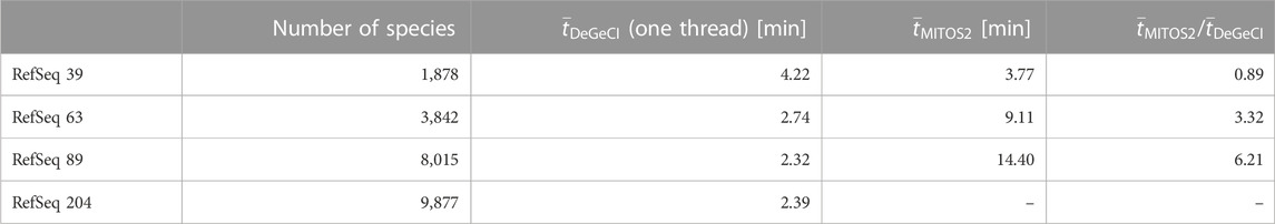
TABLE 3. Comparison of runtimes. Here, the number
Nowadays, every modern CPU offers multiple hardware threads. DeGeCI has the advantage that it can (unlike MITOS2) be run in parallel. Preliminary tests on RefSeq 89 with two threads resulted in an average runtime of 1.4 min compared to 2.32 min for one thread. This corresponds to a speed-up value of approximately 1.66 and an efficiency value of approximately 0.83.
5 Discussion
This contribution describes a new method, DeGeCI, for an efficient, automatic de novo annotation of mitochondrial genomes. The underlying reference database, which comprises a comprehensive collection of mitogenomes, is represented as a richly annotated de Bruijn graph. To generate gene predictions for an input genome sequence, DeGeCI utilizes a clustering technique that is based on the mapping information of this sequence to the graph. DeGeCI produces gene predictions of high conformity with expert-curated annotations of RefSeq, particularly showing the high precision of gene boundaries. Compared to the standard annotation tool MITOS2, DeGeCI generates predictions of at least equal quality, requires less time for annotation when using larger databases, and features better database scalability. Different from MITOS2, the new method, DeGeCI, offers a fully automated update of the reference database and can be run in parallel. Altogether, we could demonstrate that DeGeCI is well suited for large-scale annotations of mitochondrial sequence data.
5.1 Limitations
Similar to all database-based annotation approaches (e.g., MITOS, DOGMA, MOSAS, and MitoFish), DeGeCI requires a database containing annotated mitochondrial genome information that includes a certain minimum diversity of species to enable high-quality annotation of mitogenomes across a broad taxonomic spectrum. Otherwise, the annotation quality might be lower, and there might be many and/or relatively large unmapped sequence segments of the input genome. The latter leads to larger annotation times, since a comparably large amount of runtime is required to bridge these unmapped segments in the corresponding subgraph (cf. Section 2.2.2).
DeGeCI has been developed with the prior aim in mind to embed complete genomic sequences of mitochondria. These are generally generated by applying a mixture of long-read and short-read sequencing techniques. Due to the higher error rates associated with long-read sequencing data, using only long-read sequencing data for graph construction might affect the quality of gene predictions obtained using DeGeCI.
5.2 Future work
The implementation of a taxonomic filter that would allow the use of only database species of a user-supplied taxonomic classification is our agenda for future work. The use of such a filter could be advantageous with respect to annotation time or quality when a specific taxonomic group of the input sequence is known.
As discussed in Section 4.4, the result accuracy of the DeGeCI protein boundary predictions could likely be improved by scanning the proximity for start and stop codons. Since this requires the user to specify adequate genetic code tables and thus a certain degree of knowledge about the input sequence and/or user expertise, this is currently not part of DeGeCI. This could be implemented in a future version of DeGeCI, allowing the optional refinement of protein predictions.
The focus of this study has been on mitochondrial genomes. An application of the presented methods to nuclear genomes could, hence, be an interesting aspect to be explored in future studies. Suitable parameter settings for k could be determined similarly as suggested in this work.
Moreover, the implementation of a public web server version of DeGeCI is planned.
Data availability statement
Publicly available datasets were analyzed in this study. These data can be found at: https://doi.org/10.5281/zenodo.8101631 (RefSeq mitochondrial nucleotide sequences for releases 89 and 204).
Author contributions
LF, MM, and MB conceived the idea. MM and MB supervised the study and edited the manuscript. LF implemented the software, performed the computational analysis, and drafted the manuscript. All authors collaborated on the design of the algorithms and the overall workflow, the interpretation of the results, and the writing of the manuscript. All authors contributed to the article and approved the submitted version.
Funding
The research reported in this manuscript was funded by the Open Access Publishing Fund of Leipzig University supported by the German Research Foundation within the program Open Access Publication Funding. The authors further wish to thank the German Research Foundation for funding project 21210538.
Conflict of interest
The authors declare that the research was conducted in the absence of any commercial or financial relationships that could be construed as a potential conflict of interest.
Publisher’s note
All claims expressed in this article are solely those of the authors and do not necessarily represent those of their affiliated organizations, or those of the publisher, the editors, and the reviewers. Any product that may be evaluated in this article, or claim that may be made by its manufacturer, is not guaranteed or endorsed by the publisher.
Supplementary material
The Supplementary Material for this article can be found online at: https://www.frontiersin.org/articles/10.3389/fgene.2023.1250907/full#supplementary-material
Abbreviations
DeGeCI, De Bruijn graph Gene Cluster Identification; CC, connected component; FN, false negative; FP, false positive; RFD, relative frequency distribution; SGT, single genome trail.
Footnotes
1https://git.informatik.uni-leipzig.de/lfiedler/degeci
2https://doi.org/10.5281/zenodo.7010767
References
Almodaresi, F., Pandey, P., and Patro, R. (2017). “Rainbowfish: a succinct colored de Bruijn graph representation,” in 17th International Workshop on Algorithms in Bioinformatics (WABI 2017), Boston, MA, USA, August 21–23, 2017, 15. 1–18. doi:10.4230/LIPIcs.WABI.2017.18
Altschul, S. F., Gish, W., Miller, W., Myers, E. W., and Lipman, D. J. (1990). Basic local alignment search tool. J. Mol. Biol. 215, 403–410. doi:10.1016/S0022-2836(05)80360-2
Benson, D. A., Karsch-Mizrachi, I., Lipman, D. J., Ostell, J., Rapp, B. A., and Wheeler, D. L. (2000). GenBank. Nucleic Acids Res. 28, 15–18. doi:10.1093/nar/28.1.15
Bernt, M., Donath, A., Jühling, F., Externbrink, F., Florentz, C., Fritzsch, G., et al. (2013). Mitos: improved de novo metazoan mitochondrial genome annotation. Mol. Phylogenetics Evol. 69, 313–319. doi:10.1016/j.ympev.2012.08.023
Boore, J. L. (2006). Requirements and standards for organelle genome databases. OMICS A J. Integr. Biol. 10, 119–126. doi:10.1089/omi.2006.10.119
Bowe, A., Onodera, T., Sadakane, K., and Shibuya, T. (2012). “Succinct de Bruijn graphs,” in Algorithms in bioinformatics. Editors B. Raphael, and J. Tang (Berlin, Heidelberg: Springer). 225–235. doi:10.1007/978-3-642-33122-0_18
Bruijn, de, N. G. (1946). A combinatorial problem. Proc. Sect. Sci. Koninklijke Nederl. Akademie van Wetenschappen te Amsterdam 49, 758–764.
Donath, A., Jühling, F., Al-Arab, M., Bernhart, S. H., Reinhardt, F., Stadler, P. F., et al. (2019). Improved annotation of protein-coding genes boundaries in metazoan mitochondrial genomes. Nucleic acids Res. 47, 10543–10552. doi:10.1093/nar/gkz833
Eddy, S. R. (2002). A memory-efficient dynamic programming algorithm for optimal alignment of a sequence to an rna secondary structure. BMC Bioinforma. 3, 1. doi:10.1186/1471-2105-3-18
Eddy, S. R. (2011). Accelerated profile hmm searches. PLoS Comput. Biol. 7, e1002195. doi:10.1371/journal.pcbi.1002195
Eddy, S. R., and Durbin, R. (1994). RNA sequence analysis using covariance models. Nucleic Acids Res. 22, 2079–2088. doi:10.1093/nar/22.11.2079
Good, I. J. (1946). Normal recurring decimals. J. Lond. Math. Soc. s1-21, 167–169. doi:10.1112/jlms/s1-21.3.167
Iwasaki, W., Fukunaga, T., Isagozawa, R., Yamada, K., Maeda, Y., Satoh, T. P., et al. (2013). MitoFish and MitoAnnotator: a mitochondrial genome database of fish with an accurate and automatic annotation pipeline. Mol. Biol. Evol. 30, 2531–2540. doi:10.1093/molbev/mst141
Lin, Y., and Pevzner, P. A. (2014). “Manifold de Bruijn graphs,” in s in bioinformatics. Editors D. Brown, and B. Morgenstern (Berlin, Heidelberg: Springer), 296–310.
Lowe, T. M., and Eddy, S. R. (1997). tRNAscan-SE: a program for improved detection of transfer RNA genes in genomic sequence. Nucleic Acids Res. 25, 955–964. doi:10.1093/nar/25.5.955
Nawrocki, E. P., Kolbe, D. L., and Eddy, S. R. (2009). Infernal 1.0: inference of RNA alignments. Bioinformatics 25, 1335–1337. doi:10.1093/bioinformatics/btp157
Pevzner, P. A., Tang, H., and Tesler, G. (2004). De novo repeat classification and fragment assembly. Genome Res. 14, 1786–1796. doi:10.1101/gr.2395204
Pevzner, P. A., Tang, H., and Waterman, M. S. (2001). An Eulerian path approach to DNA fragment assembly. Proc. Natl. Acad. Sci. 98, 9748–9753. doi:10.1073/pnas.171285098
Pruitt, K. D., Tatusova, T., and Maglott, D. R. (2007). NCBI reference sequences (RefSeq): a curated non-redundant sequence database of genomes, transcripts and proteins. Nucleic Acids Res. 2007, D61. doi:10.1093/nar/gkl842
Sheffield, N. C., Hiatt, K. D., Valentine, M. C., Song, H., and Whiting, M. F. (2010). Mitochondrial genomics in orthoptera using mosas. Mitochondrial DNA 21, 87–104. doi:10.3109/19401736.2010.500812
Stonebraker, M. (1987). The design of the Postgres storage system. Tech. rep. California: Univ Berkeley Electronics Research Lab California.
Veith, A. d. S., and de Assuncao, M. D. (2019). Apache Spark. Cham: Springer International Publishing. doi:10.1007/978-3-319-77525-8_37
Wolstenholme, D. R. (1992). Animal mitochondrial DNA: Structure and evolution. United States: Academic Press, 173–216. doi:10.1016/S0074-7696(08)62066-5
Wyman, S. K., Jansen, R. K., and Boore, J. L. (2004). Automatic annotation of organellar genomes with DOGMA. Bioinformatics 20, 3252–3255. doi:10.1093/bioinformatics/bth352
Keywords: annotation, gene prediction, mitochondria, genome, mitogenome, Metazoa, de Bruijn graph, clustering
Citation: Fiedler L, Middendorf M and Bernt M (2023) Fully automated annotation of mitochondrial genomes using a cluster-based approach with de Bruijn graphs. Front. Genet. 14:1250907. doi: 10.3389/fgene.2023.1250907
Received: 30 June 2023; Accepted: 24 July 2023;
Published: 10 August 2023.
Edited by:
Min Zeng, Central South University, ChinaReviewed by:
Junwei Luo, Henan Polytechnic University, ChinaXingyu Liao, King Abdullah University of Science and Technology, Saudi Arabia
Copyright © 2023 Fiedler, Middendorf and Bernt. This is an open-access article distributed under the terms of the Creative Commons Attribution License (CC BY). The use, distribution or reproduction in other forums is permitted, provided the original author(s) and the copyright owner(s) are credited and that the original publication in this journal is cited, in accordance with accepted academic practice. No use, distribution or reproduction is permitted which does not comply with these terms.
*Correspondence: Lisa Fiedler, bGZpZWRsZXJAaW5mb3JtYXRpay51bmktbGVpcHppZy5kZQ==
†These authors have contributed equally to this work