 Chunlong Luo1,2
 Yang Wu
 Yi Zhao
95% of researchers rate our articles as excellent or good
Learn more about the work of our research integrity team to safeguard the quality of each article we publish.
Find out more
ORIGINAL RESEARCH article
Front. Genet. , 15 February 2023
Sec. Computational Genomics
Volume 14 - 2023 | https://doi.org/10.3389/fgene.2023.1109269
This article is part of the Research Topic Artificial Intelligence and Bioinformatics Applications for Omics and Multi-Omics Studies View all 13 articles
Chromosome segmentation is a crucial analyzing task in karyotyping, a technique used in experiments to discover chromosomal abnormalities. Chromosomes often touch and occlude with each other in images, forming various chromosome clusters. The majority of chromosome segmentation methods only work on a single type of chromosome cluster. Therefore, the pre-task of chromosome segmentation, the identification of chromosome cluster types, requires more focus. Unfortunately, the previous method used for this task is limited by the small-scale chromosome cluster dataset, ChrCluster, and needs the help of large-scale natural image datasets, such as ImageNet. We realized that semantic differences between chromosomes and natural objects should not be ignored, and thus developed a novel two-step method called SupCAM, which could avoid overfitting only using ChrCluster and achieve a better performance. In the first step, we pre-trained the backbone network on ChrCluster following the supervised contrastive learning framework. We introduced two improvements to the model. One is called the category-variant image composition method, which augments samples by synthesizing valid images and proper labels. The other introduces angular margin into large-scale instance contrastive loss, namely self-margin loss, to increase the intraclass consistency and decrease interclass similarity. In the second step, we fine-tuned the network and obtained the final classification model. We validated the effectiveness of modules through massive ablation studies. Finally, SupCAM achieved an accuracy of 94.99% with the ChrCluster dataset, which outperformed the method used previously for this task. In summary, SupCAM significantly supports the chromosome cluster type identification task to achieve better automatic chromosome segmentation.
Karyotyping is an essential cytogenetic experiment technique that aims to find numerical and structural abnormalities of chromosomes. Normally, human tissue cells have 23 pairs of chromosomes, including autosomes and sex chromosomes. These chromosomes are stained using Giemsa staining techniques and then photographed using advanced microscope cameras to generate metaphase images. The karyotyping analysis usually requires the segmentation of chromosome instances from metaphase images. Owing to the inefficiency and high cost of manual analysis, researchers have presented many automatic algorithms to ease the burden.
Most existing studies focus on the chromosome segmentation task but ignore its pre-task, chromosome cluster types identification. As non-rigid chromosomes float in an oil droplet when photographed, it is usual that touching and severely overlapping chromosomes occur in metaphase images, namely chromosome clusters. However, using classical geometric connectivity techniques, it is easy to obtain individual instances or clusters from a metaphase image. Most existing chromosome segmentation studies only dive into a specific type of chromosome cluster. To segment touching clusters, Arora (2019) and Yilmaz et al. (2018) present algorithms that make full use of the geometric characteristics between touching areas. To segment overlapping chromosome clusters, Hu et al. (2017) tries to design a new customized neural network for better performance. To segment touching-overlapping clusters, Minaee et al. (2014) dives into the geometric features of this type of cluster and proposes a geometric-based method. Alternatively, Lin et al. (2020) chooses to improve the state-of-the-art deep-learning model to tackle this issue. Nevertheless, if we can automatically identify the type of chromosome cluster first and then input it to the above segmentation methods, we can automatically segment chromosomes directly from metaphase images.
In 2021, Lin et al. (2021) proposed the chromosome cluster type identification task. In this work, 6,592 chromosome clusters were obtained from the hospital, and they created and made available the first chromosome cluster dataset (ChrCluster for simplicity). All samples are manually annotated into four categories: instance, overlapping, touching, and touching-overlapping, as shown in Figure 1. Finally, they propose a classification model as the benchmark of the ChrCluster dataset. To avoid overfitting on the small-scale ChrCluster dataset, Lin et al. (2021) takes Instagram weakly supervised learning pretrained weights [Mahajan et al. (2018)] and the customized ResNeXt [Xie et al. (2017)] classification model to achieve an accuracy of 94.09%.
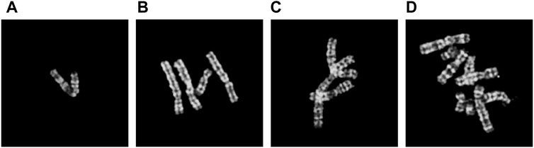
FIGURE 1. Examples of different types of chromosome clusters include (A) instance, (B) touching, (C) overlapping, and (D) touching-overlapping.
However, chromosome cluster images are gray images and only contain specific domain objects, which results in different distributions between the ChrCluster dataset and the ImageNet/Instagram dataset. Therefore, pre-training the model with the ImageNet or Instagram dataset is not the ideal option. Given this point, we attempt to pre-train domain-friendly weights only using the ChrCluster dataset for better downstream task performance.
Self-supervised contrastive learning [Wu et al. (2018); van den Oord et al. (2018); Hénaff (2020); Chen T. et al. (2020a); He et al. (2020); Chen X. et al. (2020b)] is an unsupervised learning mechanism that aims to pre-train representative features (output of specific weights) that can be transferred to downstream tasks by fine-tuning. They achieve contrastive learning through a Siamese network structure. Large-scale instance contrastive loss, such as InfoNCE, is used to attract the positive pairs and repulse the negative pairs. Specifically, they regard the different augmentation views of the same instance as positive pairs and views from different instances as negative pairs. Finally, pre-trained weights are transferred to downstream tasks, such as classification, detection, and segmentation. Supervised contrastive learning methods [Khosla et al. (2020); Cui et al. (2021); Kang et al. (2021)] are further proposed to achieve better performance on the downstream classification task. They add label information into self-supervised contrastive learning. With the help of label information, not only embeddings from the different views of the same instance should be gathered together but also embeddings of instances from the same class should be pulled close, which will result in many positives for each embedding as opposed to a single positive in self-supervised contrastive learning. Given this way, we can utilize the supervised contrastive learning framework to pre-train domain-friendly features that can capture more similarity among intraclass. However, both contrastive learning methods train the model using instance contrastive loss like the SupCon loss [Khosla et al. (2020)], which means that they are non-parametric and do not have a final FC layer as a classifier. As a result, fine-tuning at the downstream chromosome cluster identification task is essential.
For both self-supervised and supervised contrastive learning, category-invariant data augmentation approaches are essential. SimCLR [Chen T. et al. (2020a)] has systematically proved the importance of category-invariant data augmentation (RandomResizedCrop, RandomColorJittering, and GaussianBlur) for self-supervised contrastive learning. However, stronger category-variant augmentation techniques [Zhang et al. (2018); Yun et al. (2019)] are ignored due to the lack of label information. Supervised contrastive learning methods have added label information, but the instance contrastive loss they use is not yet able to adapt to continuous labels generated by previous category-variant augmentation methods. Therefore, we introduce a category-variant image composition method with discrete targets for our proposed supervised contrastive learning method, which can further enrich the visual schemas of the ChrCluster dataset and achieve better performance.
In addition, large-scale instance contrastive loss is important for supervised contrastive learning. It is obvious that the inner product of normalized embeddings in both InfoNCE [Chen T. et al. (2020a)] and SupCon [Khosla et al. (2020)] is equal to the cosine similarity operation. The angular between two embeddings is the only variable in the loss. Thus, adding an angular margin can achieve better intraclass compactness and interclass discrimination. For example, previous angular margin-based losses [Liu et al. (2016); Liu et al. (2017); Wang et al. (2018a); Wang et al. (2018b); Deng et al. (2019)] encourage sharper feature distribution and better discriminating performance by adding various angular margins between instance features and class weights. Among them, the Additive Angular Margin loss [Deng et al. (2019)] performs best. Given this way, we can design a new large-scale instance contrastive loss using additive angular margin to enhance the semantic discrimination capability of pre-trained features.
To sum up, inspired by the supervised contrastive learning method SupCon [Khosla et al. (2020)], we propose the two-step SupCAM approach to identify the various chromosome cluster types. In the first pretraining step, considering that the MoCo [He et al. (2020)] style network can save more storage space by the memory queue, we take MoCo as feature extractor to encode images. To learn category-related features, we take SupCon loss to maximize the consistency across all views of all samples in the same class rather than only that of the various views of the same sample. Additionally, we provide a category-variant image composition method to augment chromosome cluster images, which combines two randomly chosen images and assigns a new discrete label in accordance with the rule to create a new valid sample. We also import an angular margin into different embeddings of the instance contrastive loss to bring embeddings from the same class closer together. Owing to the poor synchronization between the query and the old keys, a straightforward extension that simply adds angular margins to all positive pairs may fall short of achieving model convergency. Therefore, we only import an angular margin between the different views of the same sample, known as self-margin loss, which is the first attempt to enforce more compact embeddings using large-scale instance contrastive loss with angular margin. In the second step, we fine-tune the final classification model based on the pre-trained backbone from the first step. We prove the effectiveness of our methods by fine-tuning multiple classical classification networks, such as ResNet and its variants. Overall, our main contributions in this paper can be summarized as follows:
• We solve chromosome cluster identification through a two-step method, named SupCAM, that pre-trains the backbone in a supervised contrastive learning manner and fine-tunes classification models. In this way, SupCAM obtains more representative features to avoid overfitting and domain-friendly pre-trained weights as a better alternative to ImageNet pre-trained weights.
• We propose a category-variant image composition method that will reassign the category according to the overlapping area of the chromosome clusters.
• We import angular margin into instance contrastive-based loss, named self-margin loss. The self-margin loss will enforce higher intraclass compactness and interclass discrepancy of the model.
• We prove the efficiency of our contributions through the public chromosome cluster types dataset, ChrCluster. We also achieve 94.99% accuracy, which is higher than the 94.09% accuracy proposed by Lin et al. (2021).
We will go into more depth about the suggested method in this section. In the section entitled ‘Two-Step Framework’ 2.1, we fully detail the SupCAM pre-training and fine-tuning steps and emphasize the significance of the new loss function and novel data augmentation method. The details of the new category-variant image composition approach, including the composing algorithm and principles of label assigning, will thereafter be covered in the section entitled ‘Category-Variant Image Composition’ 2.2. In the section entitled ‘Self-margin loss’ 2.3, we will deduce new self-margin loss through merging label information and angular margin step by step.
In this study, we present a two-step method called SupCAM that consists of the pre-training and fine-tuning steps, as shown in Figure 2, to tackle the chromosome cluster types classification problem. We pre-trained our backbone using the supervised contrastive learning framework in the first stage. In the second step, we extracted representative features through a pre-trained backbone and fine-tuned a few traditional classification models for final identification.
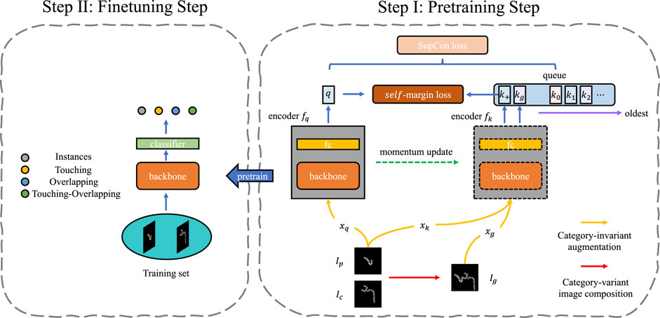
FIGURE 2. The framework of SupCAM. The pretraining step shown is based on MoCo [He et al. (2020)] structure but imports two modifications, namely category-variant image composition and self-margin loss. The fine-tuning step will initialize the backbone using weights pre-trained in the first step and finally reports identification results.
In the pre-training step, we took the MoCo as the basic architecture in this work, but it is free to be replaced with other self-supervised contrastive learning models. As shown in Figure 2, SupCAM owns query encoder fq, and key encoder fk. fq was trained in an end-to-end manner but fk was implemented as a momentum-based moving average of fq. We also inherited the dynamically updated queue but ignored the projection head used in the MoCo.
To gain multiple views of the sampled images during training, we first used category-invariant and category-variant augmentation approaches. Specifically, we randomly sampled primary image Ip and candidate image Ic. The primary images were augmented by the category-invariant augmentation methods as usual, resulting in two views with the same class, denoted as xq and xk. The Ic was first augmented using a category-variant image composition method, which combines with the Ip to create a new image, called generated image Ig. A new class label was assigned according to the look-up table. Then, the same category-invariant augmentation modules were applied on the Ig, leading to the xg. We will further describe the details of the category-variant image composition method in the category-variant image composition Section 2.2. Afterward, as shown in Figure 2, through the query encoder fq and key encoder fk, augmented samples were mapped to a tuple of representation vectors:
where key encoder fk encodes both xk and xg to embeddings k+ and kg. (q, k+) is the intrinsic positive pair as it comes from the same image, but kg is positive or negative depending on whether Ig has the same class label with Ip. Besides, k+ and kg are used to update the memory queue in a first input first output (FIFO) manner. Benefiting from the slowly progressing key encoder and progressively replaced queue, representations in the queue can remain as consistent as possible with the latest q, which helps the contrastive model converge.
Inspired by the excellent performance of angular margin loss [Liu et al. (2017); Wang H. et al. (2018b); Deng et al. (2019)], we present self-margin loss in this study for better discriminative power of the pre-trained backbone. Specifically, our final loss consisted of the SupCon loss and self-margin loss. For each query q, a set of encoded keys {k0, k1, k2, … } and k+ and kg were used to compute SupCon loss. Meanwhile, as k+ was not only the newest key compared with other keys in the memory queue but also had the same class as q, we only applied an additional angular margin between q and k+. In this way, we achieved better performance while keeping the training process stable. In Section 2.3, the analysis of the self-margin loss will be shown in detail.
All results shown in the section entitled ‘Experimental results and discussion’ 3 are from the fine-tuned classification model. As shown in Figure 2, in the fine-tuning step, we reused the pre-trained backbone network and attached a fully connected layer, a four-classes linear classifier, on top of it as our chromosome cluster types identification model. After loading the pre-trained weights of the backbone network and randomly initializing the fully connected layer, we trained the model on the training set for several epochs. In the end, we evaluated the SupCAM model on the test set for the module’s effectiveness and final performance. The details of the classification model and training process will be described in the section entitled ‘Implementation Details’ 3.3.
In this section, we will introduce a category-variant image composition algorithm as a strong data augmentation policy in SupCAM. Traditional category-invariant data augmentation methods dominate self-supervised and supervised contrastive learning methods. However, stronger category-variant data augmentation methods, such as Mixup [Zhang et al. (2018)] and CutMix [Yun et al. (2019)], are ignored because they do not satisfy the discrete targets requirements of large-scale instance contrastive loss. Thus, we propose a category-variant image composition algorithm to synthesize new chromosome cluster samples with discrete labels for enriching visual schemas.
Let (Ip, yp) and (Ic, yc) denote primary and candidate samples, respectively, where
where
Algorithm 1. Category-Variant Image Composition.
Input: primary sample (Ip, yp), candidate sample (Ic, yc), upper limit of sampling number N, pixel intersection P∩
Output: generated sample (Ig, yg)
1: Initialize yg is uncertainty and sampling count n = 0
2: W, H = Size(Ip)
3: Binary mask of Ip and Ic:
4: Bounding box of chromosome cluster in Mp and Mc:
5: Shift range of image Ip and Ic:
6: while yg is uncertainty and n < N do
7: Shift bias are uniformly sampled according to:
8: Warp the images using transformation matrix Tp and Tc:
9: Generate Ig according to the warped images through combination operation ⊕:
10: Assign label by look-up table:
11: n = n + 1
12: if yg is not uncertainty then
13: return Generated sample (Ig, yg)
14: end if
15: end while
16: return Candidate sample (Ic, yc)
As shown in Algorithm 1, we first extracted the foreground-background mask of Ip and Ic through indicator function
Here, the importance of image shift should be clarified. Unlike Mixup, which conducts linear interpolations of all pixels, and CutMix, which replaces a random image region with a patch from another image, we need to shift the image to simulate specific properties of different types of chromosome clusters. As shown in Figure 3A, chromosome clusters are commonly distributed in the central region of the image, which means that we combine images directly without random shift, leading to overlapping instances dominating the generated samples. Additionally, we should set a limited range for the shift bias. On the one hand, unlimited shifting may lead to the loss of characteristic areas, such as overlapping or touching regions. On the other hand, as shown in the invalid image illustrated in Figure 3B, most composing results may show as two individual chromosome clusters, which do not satisfy any definition of chromosome cluster types proposed by Lin et al. (2021). To determine the range of shift bias, we simplified the irregular concave polygons of chromosome clusters to rectangles of bounding boxes. Then, two bounding boxes could uniquely confirm a maximum outer enclosing box as the border of shift bias, like Figure 3C. In this way, we are much more likely to be able to generate chromosome clusters that satisfy the definition, as shown in Figure 3D.
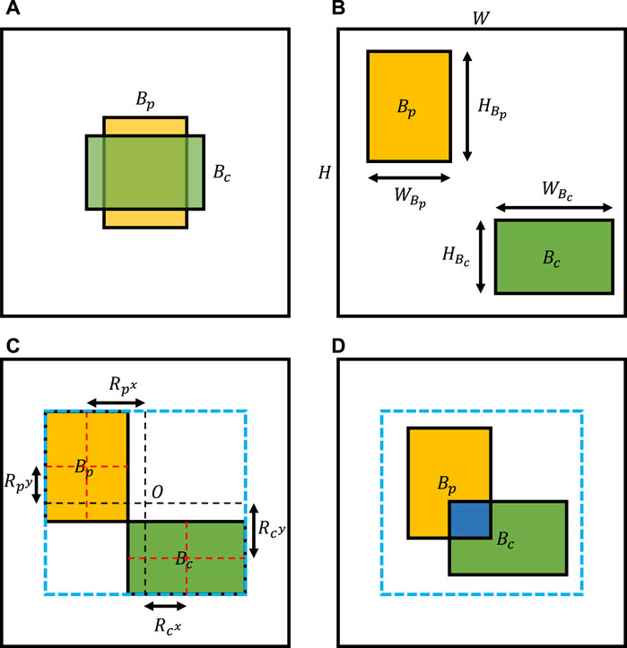
FIGURE 3. Illustration of image shift. (A) Common composing image without image shift. (B) Invalid composing image because we do not limit image shift ranges. (C) The image shift range determined by the maximum outer enclosing box of two bounding boxes. (D) Valid composing result, as we sample image shifts under a reasonable range.
In this section, we will clarify the process of assigning the correct class label to each generated sample, namely the look-up table. Considering the image composition processing and the chromosome cluster definition, the generated image will not belong to the instance category in the first place. Besides, according to Lin et al. (2021), the crucial difference between overlapping and touching chromosome clusters is whether any connectivity between two chromosome instances entails pixels intersection. However, as shown in Figure 4, it is counterintuitive if we consider these results as overlapping cases but only a few pixel intersections distribute in the pixel connectivity region. Given this point, before assigning four chromosome cluster types and an uncertainty tag, we first need to set a pixel intersection threshold P∩ greater than zero to decide whether generated image Ig is touching case
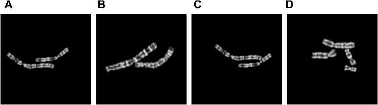
FIGURE 4. Examples of composed images with different number N of overlapping pixels. (A) N = 3; (B) N = 30; (C) N = 84; (D) N = 150.
The table in Figure 5 shows the guidance for assigning a cluster type to generated images Ig, and for simplicity, we call it middle-Table. Original categories can pair into 20 possible touching and overlapping cases. As listed in middle-Table, the left of each cell is the candidate cluster types of touching cases, and the right is the candidate cluster types of overlapping cases. Specifically, for touching cases, their class type depends on whether touching or overlapping clusters exist in original sample pairs. In other words, only if overlapping clusters exist in original sample pairs can composed touching cases be tagged as a touching-overlapping type, such as an overlapping-instance pair. Otherwise, yg should assign the touching type, such as the instance-instance pair and the touching-instance pair.
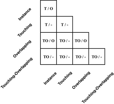
FIGURE 5. Detail of yg in the middle-Table. The left signs in each cell represent assigned labels when the number of pixel intersections of warped Ip and Ic is below or equal to the pixel intersection threshold P∩, and the right side signs represent assigned labels when pixel intersections are larger than the threshold. Furthermore, mark ’T’, ’O’, ’TO’, and ’-’ represent touching, overlapping, touching-overlapping, and uncertainty tags, respectively.
As for overlapping cases, most of the uncertainty of label yg happens in this case that the number of pixel intersections beyond pixel intersection threshold P∩. Strictly speaking, except for overlapping cases of instance-instance pair, all overlapping cases should be assigned the uncertainty tag as we cannot be sure about the number of touching and overlapping regions, such as in the light-Table described in the section entitled Category-Variant Image Composition 3.5.3. For example, given a touching-instance pair, we can assign the touching-overlapping type or the overlapping type according to the size and position of overlapping areas between two chromosome clusters. However, we should emphasize the overlapping-instance pair and the overlapping-overlapping pair. Although two pairs can be assigned the touching-overlapping type or the overlapping type, we hypothesize that when these pairs are overlapping cases, they are unlikely to have touching areas and should directly mark the overlapping type. Finally, experiment results in Table 4 support the above hypothesis.
As in the framework shown in Figure 2, we extended the InfoNCE loss to self-margin loss by gradually merging label information and additive angular margin.
Given an encoded query
where kp is the only positive key in the memory queue that q matches and KN represent the remaining negative key set.
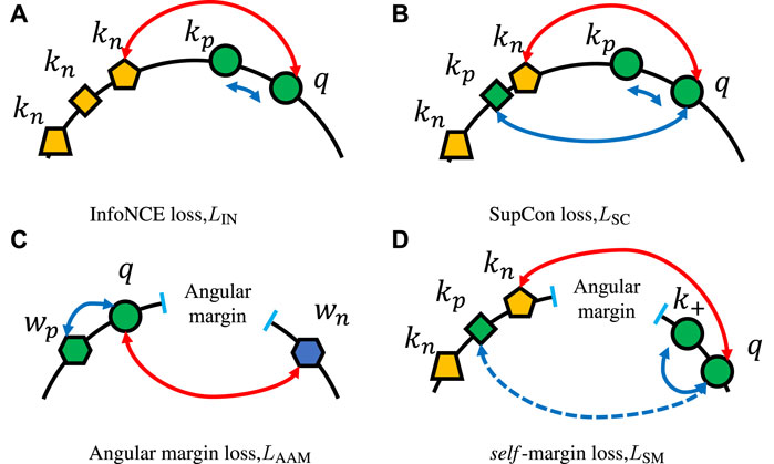
FIGURE 6. Examples of various loss functions. (A) InfoNCE loss, which pulls query q and current key kp together and regards each old embedding in the memory queue as negative key kn, which should be pushed away. (B) SupCon loss, in which not only the current key but old keys that have the same class as the query should be pulled close. The example of angular margin loss in (C) shows how hard margin constrains parametric weights and makes the same class embeddings more compact. (D) Depiction of our self-margin loss, which only enforces the angular margin between the query and the current key and ignores other positive keys in the memory queue.
Different from only augmented views of the same image should be considered as positives in InfoNCE loss, SupCon loss LSC as shown in Figure 6B, imports label information and generalizes to an arbitrary number of positives as long as they belong to the same class:
where KP is a set of positive keys that have the same class label as query q. The SupCon loss function can be regarded as the average of multiple times of InfoNCE loss value, as each kp can be considered as the only positive key at some point. The loss encourages the encoder to pull embeddings of the same class closer, resulting in a more reasonable distribution of representations for the subsequent supervised learning task.
Now we move on to the additive angular margin loss LAAM proposed in ArcFace [Wang F. et al. (2018a)]. As illustrated in Figure 6C, a larger angular margin, which exists between q and negative class weight wn, will enforce the same class queries q closer and make them easily identifiable. We suppose we have normalized weights
where
If we set wp = kp, WN = KN, and wi = ki in LAAM, then from Eqs 4, 5 we have self-margin loss LSM:
However, LAAM relies on parametric weights from the last fully connected layer. These weight vectors are the latest and are smoothly updated by end-to-end backpropagation, which results in enough synchronization between embeddings and weights. On the contrary, although a slowly evolving key encoder exists, all keys used in contrastive losses (such as LIN and LSC) are non-parametric and rapidly changing in a FIFO manner. Given this point, positive keys are consistent enough for the contrastive-based loss but not synchronized enough for the angular margin-based loss. We cannot even make the model converge using Eq. 6.
As shown in Figure 2, the synchronization between query q and positive key k+ ∈ KP has been guaranteed by the similar weights (moving-average key encoder fk and the same batch). Therefore, in Eq. 6, for query q, we only hold on to the latest inherent positive key k+ and ignore the remaining positive keys, including possible kg. The final formulation of self-margin loss LSM is:
and illustrated in Figure 6D.
We will prove the performance of LSM in Experiments 3.5 and compare it with some intuitive candidate methods.
In this study, we used the dataset reported by Lin et al. (2021) to evaluate our model performance and demonstrate the effectiveness of modules. The dataset is the first clinical chromosome cluster dataset that has 6,592 samples, called ChrCluster. All samples are padded to the 224 × 224 size and manually labeled into four categories: 1,712 chromosome instance, 3,029 touching chromosomes cluster, 1,038 overlapping chromosomes cluster, and 813 touching-overlapping chromosomes cluster. In the ablation study Section 3.5, we described how we split the dataset into 3,955 training samples, 659 validation samples, and 1,978 test samples in a class-based random stratified fashion. For the final comparison in the Section entitled ‘Comparison Result’ 3.4, we followed the division principle described by Lin et al. (2021), which has 80% training data, 10% validation data, and 10% test data. To avoid leaking test set information from the pre-training step to the fine-tuning step, we pre-trained the backbone network only using the training set no matter whether the goal is an ablation study or final comparisons.
To fairly evaluate the performance of SupCAM, we followed the main evaluation metrics described by Lin et al. (2021) including accuracy, precision, sensitivity, specificity, and F1. It is worth noticing that except for the accuracy, all the above-mentioned metrics were averaged in a ‘macro’ fashion. The ‘macro’ fashion will first calculate metrics for each category individually and then average the metrics across classes with equal weights.
Now, we should clarify the definition of the following four basic criteria in a multi-classification task:
• True positive(TPi): given a test sample that belongs to i-th class, if the model correctly predicts it as i-th class, we regard it as true positive.
• False positive(FPi): given a test sample that does not belong to i-th class, if the model incorrectly predicts it as i-th class, we regard it as false positive.
• False negative(FNi): given a test sample that belongs to i-th class, if the model incorrectly predicts it as other classes, we regard it as false negative.
• True negative(TNi): given a test sample that does not belong to i-th class, if the model correctly predicts it as other classes, we regard it as true negative.
Assume that Nc represents the number of chromosome cluster categories and N is the number of test set instances, then we have:
All above-mentioned metrics are as higher as better. We use percentages for them and keep two decimal places.
We implemented our work on the Pytorch Lightning1 toolbox based on the Pytorch [Paszke et al. (2019)] deep-learning library. We finished all experiments on an Ubuntu OS Server with one NVIDIA GTX Titan Xp GPU.
In the first pre-training phase, following the MoCo pipeline, we optimized the structure and some hyperparameters for the chromosome cluster type identification task. As described in the two-step framework Section 2.1, besides the conventional query q and key k+ used in MoCo, we additionally generated xg using the category-variant image composition method and encoded it as the third embedding kg through the key encoder. Limited by the size of the dataset, we reduced the embedding dimension to 128-d and the queue capacity to 1,024 accordingly. The scalar temperature τ used in SupCon loss and self-margin loss was set as 0.07. We chose 0.2 for angular margin m and 200 for pixel intersection hyperparameter P∩. We used SGD as our optimizer, where momentum is 0.9, and weight decay is 0.0001. We set the mini-batch size as 32 for the single GPU and trained the model for 200 epochs. Furthermore, we applied linear warm-up during the first 20 epochs until achieving the initial learning rate 0.03 and then decayed it through a cosine annealing schedule. Category-invariant image augmentation methods used in the first step included RandomResizedCrop and HorizontalFlip. The total loss is the sum of SupCon loss LSC and self-margin loss LSM:
In the second fine-tuning step, for the classification model, we first loaded the corresponding pre-trained backbone module and randomly initialized the weights and bias of the final classifier. Only RandomRotate was employed during the training phase to reduce overfitting. We used SGD as our optimizer and had the same setting as the pre-training step. We trained the classification model for 15 epochs with a mini-batch of 16 images. Unlike the first step, the initial learning rate was set as 0.01 and decreased by 0.1 after 8 and 12 epochs individually. The loss function adopted in the fine-tuning step was cross-entropy loss enhanced by label smoothing (hyperparameter σ = 0.1) [Szegedy et al. (2016)].
In this section, we report the final results following the division principle of Lin et al. (2021). Table 1 shows the comparison results between SupCAM and previous methods. On the top of Table 1, we list some representative experiment results of previous methods with different backbones, including ResNet101 [He et al. (2016)], DenseNet121 [Huang et al. (2017)], and ResNeXt101 [Xie et al. (2017)]. Specifically, ResNeXt† optimizes the header of the classification model using a mixed pooling layer and multiple linear-dropout groups. Meanwhile, not only 1.28 million images from the ImageNet dataset but also approximately 940 million images from the Instagram dataset are used to pre-train backbone weights, which are loaded as initial weights of the ResNeXt†. Owing to above-mentioned improvements, ResNeXt† proposed by Lin et al. (2021) achieves the previous state-of-the-art performance, which is 94.09 accurate and has the best results with other evaluation metrics.
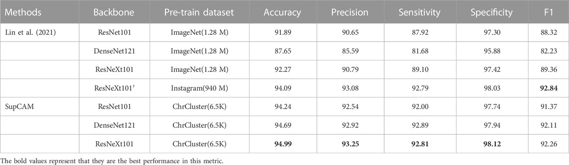
TABLE 1. Comparison with previous methods. All experiments were conducted following the division principle in Lin et al. (2021). ResNeXt101: ResNeXt101 32 × 8d; †: ResNeXt101-32 × 8d attached with a customized header network invented by Lin et al. (2021); ImageNet: 1.28 million images with 1,000-class ImageNet dataset; Instagram: 940 million public images with a
In this study, benefiting from the supervised contrastive learning framework enhanced by the category-variant image composition methods and self-margin loss, SupCAM achieved the best performance. Specifically, SupCAM improved the accuracy by a large margin of 2.35 under ResNet101 and 2.72 under the original ResNeXt101. Finally, although Lin et al. (2021) used an extremely large Instagram dataset, which was almost 140,000 times larger than ChrCluster, we still increased the accuracy by approximately 0.9 compared with ResNeXt†. Except for F1, other metrics also performed better. It is worth noting that previous methods may suffer from heavy overfitting, as shown in the result that used the DenseNet121 as the backbone network in Lin et al. (2021). As a more powerful backbone than ResNet101, DenseNet121 performed less well in all metrics. By contrast, under SupCAM, DenseNet121 successfully outperformed ResNet101, which means that SupCAM can alleviate the risk of overfitting without relying on a large dataset but using only the ChrCluster dataset. To sum up, Table 1 shows the high data utilization efficiency and robustness of the SupCAM for solving the task of chromosome cluster type identification. In addition, we evaluated the performance using pre-trained weights from ImageNet instead of random initialization in the first step of SupCAM, and as shown in Supplementary Table S1, it also outperformed the previous method, but was worse than the final SupCAM.
Besides the above metrics across classes, we used a confusion matrix to further reveal the performance of the SupCAM method in each class. As shown in Figure 7, SupCAM outperformed a previous study [Lin et al. (2021)] on instance, overlapping, and touching-overlapping classes but was weak in the overlapping category. Specifically, the number of touching-overlapping clusters incorrectly predicted as touching and overlapping types were reduced simultaneously, which resulted in an increment of 3.66 in the accuracy of the touching-overlapping class. Additionally, the accuracy of the instance class and the touching class was increased to 99.42 and 96.04, respectively. It is obvious that the combination of the category-variant image composition method and self-margin loss can improve the performance of the identification model in most chromosome cluster categories.
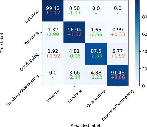
FIGURE 7. The first line of each cell is the confusion matrix of SupCAM with ResNeXt101 backbone on the test set. Besides, on the second line of each cell, we show differences between Lin et al. (2021) and our method, in which red and green represent increment or decrement of percentage, respectively.
At the same time, to try to explain the degeneracy of SupCAM in the overlapping category, we list some false negative samples, especially those misclassified as the instance type. As illustrated by Figure 8, they are puzzling samples, and it is hard to decide whether they belong to the overlapping type at first glance. On the other side, a hard threshold of pixel intersection in the category-variant image composition method may import artificial disturbance to the label system, which adds confusion to the final prediction. Therefore, these weaknesses inspire us to propose more reasonable and natural image composition methods in the future.
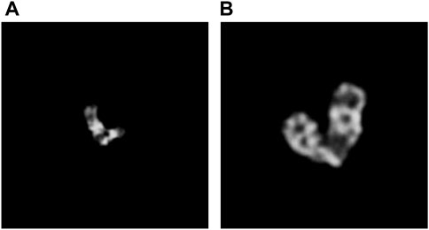
FIGURE 8. Overlapping clusters are misclassified as the instance class by SupCAM. (A) shows a misclassified example where the bottom of the left chromosome occludes the other one. (B) is another misclassified example where the bottom of the right chromosome occludes the bottom of the left one.
To evaluate the effectiveness of each model, we applied the ablation study at the 30% test set of the ChrCluster dataset. To avoid performance fluctuations due to the small size of the dataset, all experiments during the ablation study were repeated 10 times and we obtained the mean and standard deviation of each evaluation metric. In this way, as well as comparing the performance through the mean value, we can further justify the stableness of each method.
As shown in Table 2, we first trained the chromosome cluster types classification model from scratch as the baseline, which was 88.38 ± 0.60 accurate. Pre-training on the large ImageNet dataset further improved the accuracy to 92.65 ± 0.30. However, the above experiments suffer from larger performance fluctuation than our methods, which reminds us that a huge domain gap exists between the ImageNet and ChrCluster. Therefore, pre-training the chromosome cluster types identification model on the large ImageNet dataset is not the best choice. Finally, we proved that the key factor driving the model performance improvement is the model structure itself as SupCAM achieved the best performance among all experiments under the same fine-tuning strategies.
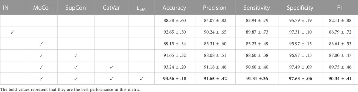
TABLE 2. Ablation study of the SupCAM model with ResNet50 on the 30% test set of the ChrCluster dataset. We repeated all experiments 10 times and report the mean and standard deviation. IN indicates that the backbone network has been pre-trained by the ImageNet dataset. CatVar, category-variant image composition method; LSM, self-margin loss.
To verify the contribution of supervised contrastive learning to the performance, before completing the basic classification task, we imported the pre-training step, which pre-trained the backbone in a supervised contrastive manner with SupCon loss through MoCo architecture. We took the MoCo augmentation setting [Chen X. et al. (2020b)] as the initial augmentation method in this experiment. Table 2 shows that the MoCo-style supervised contrastive pre-training step increased accuracy by 3.27 points and had a F1 score 4.89 points higher than the model trained from scratch. It is notable here that the direct employment of the MoCo-style supervised contrastive pre-training step was worse than the identification model pre-trained by the ImageNet dataset, but it was more stable in some cases. In conclusion, pre-training the backbone in a supervised contrastive manner is effective but we need more specific optimizations to adapt the chromosome cluster types identification task.
The experiment results in Table 2 show that the category-variant image composition method improves accuracy from 91.65 ± 0.32 to 93.25 ± 0.20 and specificity from 96.97 ± 0.13 to 97.49 ± 0.09. Both the performance and stableness of this model were increased and even outperformed the model trained by the MoCo setting, which validates that the category-variant image composition method can more reasonably and effectively augment chromosome cluster data than the original MoCo augmentation setting.
To be more specific, as shown in Supplementary Figure S1, we experimented with multiple candidate pixel intersection threshold P∩, and box plots show that when the P∩ is set as 200 pixels, the model achieves the best performance in all metrics. Meanwhile, we also examined the choices of composition methods in overlapping areas, as shown in Table 3. Besides the equal weights method used in this study, we list two representative composition methods. Linear interpolation through a sampled λ ∼B(1,1) is widely used in Yun et al. (2019) and Zhang et al. (2018). Another straightforward idea is taking the maximum pixel value from the primary image Ip and the candidate image Ic as the final pixel in overlapping areas. Experiments show that the ‘maximum’ method is not suitable for the chromosome cluster types identification task and the ”λ-interpolation” method performs badly on the most important accuracy criterion, although slightly outperforms the ‘equal weights’ method on other metrics.
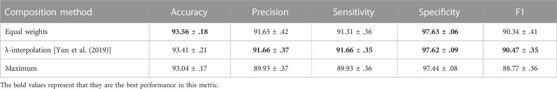
TABLE 3. Ablation study of composition methods. Equal weights mean that the overlapping area of Ip and Ic are combined half and half. λ shows that we sampled a λ from beta distribution and then applied linear interpolations in the overlapping areas of two images. The final maximum experiment represents the operation of taking the maximum pixel value in overlapping areas.
Furthermore, we confirmed the design of the look-up table in Table 4. As shown in the results, the middle-Table scheme achieved the best performance. In addition, we evaluated some extreme scenarios, such as the heavy-Table scheme and the light-Table scheme. Specifically, the heavy-Table scheme assigns an explicit label to each (Ip, Ic) pair directly no matter whether disagreements exist in overlapping cases. Suppose there is a touching-instance pair in an overlapping case, the middle-Table will tag them with an uncertainty label, but with a heavy-Table, we roughly assign the touching-overlapping category. The light-Table solution takes the opposite approach by not providing any valid label for overlapping cases unless they all belong to the instance type. The results in Table 4 show that the heavy-Table achieved an accuracy of 93.30 ± .28, which outperformed the 93.09 ± .11 accuracy of the light-Table scheme. Through the comparison between light-middle-heavy solutions, we can conclude that 1) category-variant image composition method indeed improves the performance of the cluster type identification task
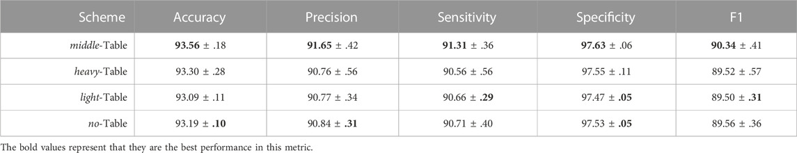
TABLE 4. Ablation study of the look-up table. Besides the middle-Table, which was our final choice, we tried to extend the label assigning to the extreme, namely through the heavy-Table and light-Table schemes. The goal of the no-Table is to examine the effects of candidate image Ic.
Moreover, to clarify the effects of taking Ic as Ig as in line 16 of Algorithm 1; Table 4 shows the results from a contrast experiment we conducted, called a no-Table scheme, that only used existing candidate image Ic rather than composed images. As expected, no-Table achieved an accuracy of 93.19 ± .10, which was lower but more stable than that of middle-Table, proving the effectiveness and relative unstableness of the category-variant image composition method once more.
As shown in Table 2, self-margin loss improved the accuracy from 93.24 ± .20 to 93.56 ± .18 and the precision, sensitivity, specificity, and F1 scores were also improved. Besides, it is worth noting that weights pre-trained with self-margin loss could further stabilize the final classification performance. Thus, we validated the effectiveness of self-margin loss of the first pre-training step.
It is important to find the optimal margin m for the chromosome cluster types identification task, and the best margin m observed in Table 5 was 0.2. Specifically, smaller additional angular margin penalties, such as m = 0.1 and m = 0.2, improved the performance. However, when margin penalties was large, e.g., m = 0.3 and m = 0.4, self-margin loss not only decreased the performance but also made the model more unstable. When the margin penalty increased to 0.5, the model could not be converged. Therefore, we conclude that although we ensure synchronization by (q, k+) pair, the moving-average update manner makes the model more sensitive to the large margin penalty than the model updated in an end-to-end manner, which is further described in the next paragraph.
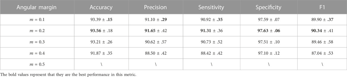
TABLE 5. The table below shows SupCAM performance with different angular margin values (m in Eq. 7) used in the self-margin loss during the first pre-training step.
Furthermore, margin-based architectures are diverse, and we justified the advantages of self-margin loss through the results shown in Table 6. As illustrated in Figure 9A, with ‘parametric margin’ as one of the candidate schemes, we additionally added an end-to-end updating weight
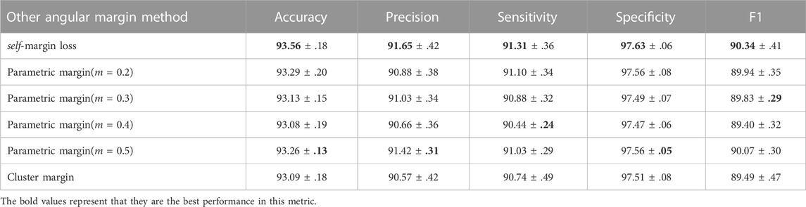
TABLE 6. Other candidate angular margin based scenarios and the main differences are detailed in Section 3.5.4.
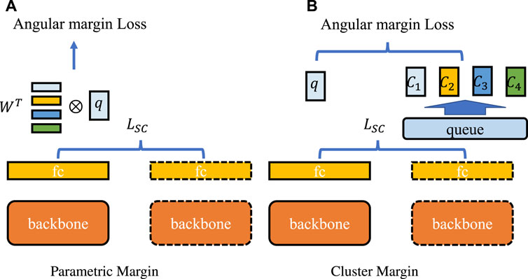
FIGURE 9. Comparison of margin-based methods. The backbone network is shared between the first and second steps, and the fully connected layer outputs queries and keys. The dashed lines indicate that all layers are updated in a moving-average manner. LSC represents SupCon loss. (A) represents the “parametric margin” schema which applies angular margin loss between query embedding and additional parametric weights W. (B) is the “cluster margin” method that clusters all key embeddings into four class centers {C1, C2, C3, C4} according to class label, and applies angular margin between query embeddings and cluster centers.
In this study, we proposed a two-step SupCAM method to solve the chromosome cluster types identification task. In the first step, we improved the supervised contrastive learning method through a strong category-variant image composition algorithm and self-margin loss. After pre-training, we further fine-tuned the classification models in the second step. The effectiveness of each module was proved by massive ablation studies. The top prediction performance suggested that SupCAM has state-of-the-art performance in the chromosome cluster identification task. All these experimental findings demonstrate that the proposed SupCAM, as a supervised contrastive learning method, can effectively extract more representative and domain-friendly weights from the small-scale ChrCluster and is a better alternative to previous ImageNet pre-trained weights as it alleviates overfitting risks, resulting in better performance. Specifically, SupCAM introduces a strong category-variant image composition method with discrete labels to generate more abundant visual schemas. Meanwhile, we designed and implemented a new stable self-margin loss by adding an angular margin between the different embeddings of the instance contrastive loss, resulting in higher intraclass compactness and interclass discrepancy. Although our study focuses on chromosome cluster identification, our proposed method can inspire more researchers to analyze medical images using only small-scale medical image datasets rather than large natural image datasets. In the future, we will refine image composition processing and the look-up table to achieve more stable performance. In addition, other schemes that add angular margin into instance contrastive-based loss should be further studied.
Publicly available datasets were analyzed in this study. This data can be found here: [https://github.com/ChengchuangLin/ChromosomeClusterIdentification].
CL, YW, and YZ contributed to conception and design of the study. CL and YW analyzed the dataset. CL performed the model experiments. CL wrote the first draft of the manuscript. All authors contributed to the manuscript revision and read and approved the submitted version.
This work was supported by the Institute of Computing Technology, Chinese Academy of Sciences (55E161080).
We thank Dr. Lianhe Zhao for correcting the article grammar and some spelling errors, and PhD student Yufan Luo for his comments on the Introduction section and Category-variant image composition section.
The authors declare that the research was conducted in the absence of any commercial or financial relationships that could be construed as a potential conflict of interest.
All claims expressed in this article are solely those of the authors and do not necessarily represent those of their affiliated organizations, or those of the publisher, the editors and the reviewers. Any product that may be evaluated in this article, or claim that may be made by its manufacturer, is not guaranteed or endorsed by the publisher.
The Supplementary Material for this article can be found online at: https://www.frontiersin.org/articles/10.3389/fgene.2023.1109269/full#supplementary-material
1https://pytorch-lightning.readthedocs.io/en/latest/
Arora, T. (2019). A novel approach for segmentation of human metaphase chromosome images using region based active contours. Int. Arab. J. Inf. Technol. 16, 132–137.
Chen, T., Kornblith, S., Norouzi, M., and Hinton, G. E. (2020a). “A simple framework for contrastive learning of visual representations,” in Proceedings of the 37th International Conference on Machine Learning, ICML 2020, Virtual Event (PMLR), 13-18 July 2020 (Vienna, Austria: PMLR), 1597–1607. vol. 119 of Proceedings of Machine Learning Research.
Chen, X., Fan, H., Girshick, R. B., and He, K. (2020b). Improved baselines with momentum contrastive learning. CoRR abs/2003.04297.
Cui, J., Zhong, Z., Liu, S., Yu, B., and Jia, J. (2021). “Parametric contrastive learning,” in 2021 IEEE/CVF International Conference on Computer Vision, ICCV 2021, October 10-17, 2021 (Montreal, QC, Canada: IEEE), 695–704. doi:10.1109/ICCV48922.2021.00075
Deng, J., Guo, J., Xue, N., and Zafeiriou, S. (2019). “Arcface: Additive angular margin loss for deep face recognition,” in IEEE Conference on Computer Vision and Pattern Recognition, CVPR 2019, June 16-20, 2019 (Long Beach, CA, USA: Computer Vision Foundation/IEEE), 4690–4699. doi:10.1109/CVPR.2019.00482
He, K., Fan, H., Wu, Y., Xie, S., and Girshick, R. B. (2020). “Momentum contrast for unsupervised visual representation learning,” in 2020 IEEE/CVF Conference on Computer Vision and Pattern Recognition, CVPR 2020, June 13-19, 2020 (Seattle, WA, USA: Computer Vision Foundation/IEEE), 9726–9735. doi:10.1109/CVPR42600.2020.00975
He, K., Zhang, X., Ren, S., and Sun, J. (2016). “Deep residual learning for image recognition,” in 2016 IEEE Conference on Computer Vision and Pattern Recognition, CVPR 2016, June 27-30, 2016 (Las Vegas, NV, USA: IEEE Computer Society), 770–778. doi:10.1109/CVPR.2016.90
Hénaff, O. J. (2020). “Data-efficient image recognition with contrastive predictive coding,” in Proceedings of the 37th International Conference on Machine Learning, ICML 2020, Virtual Event (PMLR), vol. 119 of Proceedings of Machine Learning Research, 13-18 July 2020 (Vienna, Austria: PMLR), 4182–4192.
Hu, R. L., Karnowski, J., Fadely, R., and Pommier, J. (2017). Image segmentation to distinguish between overlapping human chromosomes. CoRR abs/1712.07639.
Huang, G., Liu, Z., van der Maaten, L., and Weinberger, K. Q. (2017). “Densely connected convolutional networks,” in 2017 IEEE Conference on Computer Vision and Pattern Recognition, CVPR 2017, July 21-26, 2017 (Honolulu, HI, USA: IEEE Computer Society), 2261–2269. doi:10.1109/CVPR.2017.243
Kang, B., Li, Y., Xie, S., Yuan, Z., and Feng, J. (2021). “Exploring balanced feature spaces for representation learning,” in 9th International Conference on Learning Representations, ICLR 2021, Virtual Event, May 3-7, 2021 (Austria: OpenReview.net).
Khosla, P., Teterwak, P., Wang, C., Sarna, A., Tian, Y., Isola, P., et al. (2020). “Supervised contrastive learning,” in Advances in Neural Information Processing Systems 33: Annual Conference on Neural Information Processing Systems 2020, NeurIPS 2020, virtual, December 6-12, 2020.
Lin, C., Zhao, G., Yin, A., Ding, B., Guo, L., and Chen, H. (2020). As-panet: A chromosome instance segmentation method based on improved path aggregation network architecture. J. Image Graph. 25, 2271–2280.
Lin, C., Zhao, G., Yin, A., Yang, Z., Guo, L., Chen, H., et al. (2021). A novel chromosome cluster types identification method using resnext WSL model. Med. Image Anal. 69, 101943. doi:10.1016/j.media.2020.101943
Liu, W., Wen, Y., Yu, Z., Li, M., Raj, B., and Song, L. (2017). “Sphereface: Deep hypersphere embedding for face recognition,” in 2017 IEEE Conference on Computer Vision and Pattern Recognition, CVPR 2017, July 21-26, 2017 (Honolulu, HI, USA: IEEE Computer Society), 6738–6746. doi:10.1109/CVPR.2017.713
Liu, W., Wen, Y., Yu, Z., and Yang, M. (2016). “Large-margin softmax loss for convolutional neural networks,” in Proceedings of the 33nd International Conference on Machine Learning, ICML 2016, June 19-24, 2016 (New York City, NY, USA: JMLR.org), 507–516. vol. 48 of JMLR Workshop and Conference Proceedings.
Mahajan, D., Girshick, R. B., Ramanathan, V., He, K., Paluri, M., Li, Y., et al. (2018). “Exploring the limits of weakly supervised pretraining,” in Computer Vision - ECCV 2018 - 15th European Conference, September 8-14, 2018 (Munich, Germany: Springer), 185–201. Proceedings, Part II. vol. 11206 of Lecture Notes in Computer Science. doi:10.1007/978-3-030-01216-8_12
Minaee, S., Fotouhi, M., and Khalaj, B. H. (2014). “A geometric approach to fully automatic chromosome segmentation,” in 2014 IEEE Signal Processing in Medicine and Biology Symposium (SPMB), 20 July 2015 (Philadelphia, PA, USA: IEEE), 1–6. doi:10.1109/SPMB.2014.7163174
Paszke, A., Gross, S., Massa, F., Lerer, A., Bradbury, J., Chanan, G., et al. (2019). “Pytorch: An imperative style, high-performance deep learning library,” in Advances in Neural Information Processing Systems 32: Annual Conference on Neural Information Processing Systems 2019, NeurIPS 2019, Vancouver, BC, Canada, December 8-14, 2019, 8024–8035.
Szegedy, C., Vanhoucke, V., Ioffe, S., Shlens, J., and Wojna, Z. (2016). “Rethinking the inception architecture for computer vision,” in 2016 IEEE Conference on Computer Vision and Pattern Recognition, CVPR 2016, June 27-30, 2016 (Las Vegas, NV, USA: IEEE Computer Society), 2818–2826. doi:10.1109/CVPR.2016.308
van den Oord, A., Li, Y., and Vinyals, O. (2018). Representation learning with contrastive predictive coding. CoRR abs/1807.03748.
Wang, F., Cheng, J., Liu, W., and Liu, H. (2018a). Additive margin softmax for face verification. IEEE Signal Process. Lett. 25, 926–930. doi:10.1109/LSP.2018.2822810
Wang, H., Wang, Y., Zhou, Z., Ji, X., Gong, D., Zhou, J., et al. (2018b). “Cosface: Large margin cosine loss for deep face recognition,” in 2018 IEEE Conference on Computer Vision and Pattern Recognition, CVPR 2018, June 18-22, 2018 (Salt Lake City, UT, USA: Computer Vision Foundation/IEEE Computer Society), 5265–5274. doi:10.1109/CVPR.2018.00552
Wu, Z., Xiong, Y., Yu, S. X., and Lin, D. (2018). “Unsupervised feature learning via non-parametric instance discrimination,” in 2018 IEEE Conference on Computer Vision and Pattern Recognition, CVPR 2018, June 18-22, 2018 (Salt Lake City, UT, USA: Computer Vision Foundation/IEEE Computer Society), 3733–3742. doi:10.1109/CVPR.2018.00393
Xie, S., Girshick, R. B., Dollár, P., Tu, Z., and He, K. (2017). “Aggregated residual transformations for deep neural networks,” in 2017 IEEE Conference on Computer Vision and Pattern Recognition, CVPR 2017, July 21-26, 2017 (Honolulu, HI, USA: IEEE Computer Society), 5987–5995. doi:10.1109/CVPR.2017.634
Yilmaz, I. C., Yang, J., Altinsoy, E., and Zhou, L. (2018). “An improved segmentation for raw g-band chromosome images,” in 5th International Conference on Systems and Informatics, ICSAI 2018, November 10-12, 2018 (Nanjing, China: IEEE), 944–950. doi:10.1109/ICSAI.2018.8599328
Yun, S., Han, D., Chun, S., Oh, S. J., Yoo, Y., and Choe, J. (2019). “Cutmix: Regularization strategy to train strong classifiers with localizable features,” in 2019 IEEE/CVF International Conference on Computer Vision, ICCV, October 27 - November 2, 2019 (Seoul, Korea (South): IEEE), 6022–6031. doi:10.1109/ICCV.2019.00612
Keywords: supervised contrastive learning, category-variant data augmentation, angular margin loss, chromosome cluster types identification, karyotyping
Citation: Luo C, Wu Y and Zhao Y (2023) SupCAM: Chromosome cluster types identification using supervised contrastive learning with category-variant augmentation and self-margin loss. Front. Genet. 14:1109269. doi: 10.3389/fgene.2023.1109269
Received: 27 November 2022; Accepted: 25 January 2023;
Published: 15 February 2023.
Edited by:
Angelo Facchiano, Institute of Food Sciences (CNR), ItalyReviewed by:
Jiaogen Zhou, Huaiyin Normal University, ChinaCopyright © 2023 Luo, Wu and Zhao. This is an open-access article distributed under the terms of the Creative Commons Attribution License (CC BY). The use, distribution or reproduction in other forums is permitted, provided the original author(s) and the copyright owner(s) are credited and that the original publication in this journal is cited, in accordance with accepted academic practice. No use, distribution or reproduction is permitted which does not comply with these terms.
*Correspondence: Yi Zhao, YmlvenlAaWN0LmFjLmNu
Disclaimer: All claims expressed in this article are solely those of the authors and do not necessarily represent those of their affiliated organizations, or those of the publisher, the editors and the reviewers. Any product that may be evaluated in this article or claim that may be made by its manufacturer is not guaranteed or endorsed by the publisher.
Research integrity at Frontiers
Learn more about the work of our research integrity team to safeguard the quality of each article we publish.