 Yang Da
 Zuoxiang Liang
 Dzianis Prakapenka
- Department of Animal Science, University of Minnesota, Saint Paul, MN, United States
The rapid growth in genomic selection data provides unprecedented opportunities to discover and utilize complex genetic effects for improving phenotypes, but the methodology is lacking. Epistasis effects are interaction effects, and haplotype effects may contain local high-order epistasis effects. Multifactorial methods with SNP, haplotype, and epistasis effects up to the third-order are developed to investigate the contributions of global low-order and local high-order epistasis effects to the phenotypic variance and the accuracy of genomic prediction of quantitative traits. These methods include genomic best linear unbiased prediction (GBLUP) with associated reliability for individuals with and without phenotypic observations, including a computationally efficient GBLUP method for large validation populations, and genomic restricted maximum estimation (GREML) of the variance and associated heritability using a combination of EM-REML and AI-REML iterative algorithms. These methods were developed for two models, Model-I with 10 effect types and Model-II with 13 effect types, including intra- and inter-chromosome pairwise epistasis effects that replace the pairwise epistasis effects of Model-I. GREML heritability estimate and GBLUP effect estimate for each effect of an effect type are derived, except for third-order epistasis effects. The multifactorial models evaluate each effect type based on the phenotypic values adjusted for the remaining effect types and can use more effect types than separate models of SNP, haplotype, and epistasis effects, providing a methodology capability to evaluate the contributions of complex genetic effects to the phenotypic variance and prediction accuracy and to discover and utilize complex genetic effects for improving the phenotypes of quantitative traits.
Introduction
Genomic estimation of variance components and associated heritabilities and genomic prediction for quantitative traits using single nucleotide polymorphism (SNP) markers and mixed models have become a widely used approach for genetic improvement in livestock and crop species. The rapid growth in genomic selection data provides unprecedented opportunities to discover and utilize complex genetic mechanisms, but methodology and computing tools are lacking for investigating complex genetic mechanisms using the approach of genomic estimation and prediction. The integration of global low-order epistasis effects and local high-order epistasis effects contained in haplotypes for genomic estimation and prediction is a step forward for the discovery and application of complex genetic mechanisms to improve the phenotypes of quantitative traits.
The theory of genetic partition of two-locus genotypic values defines four types of epistasis values: additive × additive (A×A), additive × dominance (A×D), dominance × additive (D×A), and dominance × dominance (D×D) epistasis values (Cockerham, 1954; Kempthorne, 1954). The Cockerham method defines each epistasis coefficient as the product of the coefficients of the two interacting effects that each can be an additive or dominance effect (Cockerham, 1954). This definition of epistasis coefficient is the basis for defining epistasis model matrices in terms of the model matrices of additive and dominance effects. Cockerham also defines a pedigree epistasis relationship as the product between the pedigree additive and dominance relationships (Cockerham, 1954), and this definition is the theoretical basis for Henderson’s approach to express epistasis relationship matrices as the Hadamard products of the additive and dominance relationship matrices (Henderson, 1985). Henderson’s Hadamard products for epistasis relationship matrices were suggested for genomic prediction using epistasis effects by replacing the pedigree additive and dominance relationship matrices with the genomic additive and dominance relationship matrices calculated from SNP markers (Su et al., 2012; Muñoz et al., 2014; Vitezica et al., 2017). This genomic version of Henderson’s Hadamard products avoids the use of large epistasis model matrices that can be difficult or impossible to compute but contains intra-locus epistasis effects that are not present in the epistasis model (Martini et al., 2020). For this reason, the genomic version of Henderson’s Hadamard products could be described as approximate genomic epistasis relationship matrices (AGERM). Formulations have been developed to obtain the exact genomic epistasis relationship matrices (EGERM) that remove the intra-locus epistasis effects in AGERM by modifying Henderson’s Hadamard products without creating the epistasis model matrices (Jiang and Reif, 2015; Martini et al., 2016; Jiang and Reif, 2020; Martini et al., 2020). The difference between AGERM and EGERM tends to diminish as the number of SNPs increases (Jiang and Reif, 2020). Henderson’s Hadamard products and hence AGERM are applicable to any order of epistasis effects, and EGERM also has a general formula for any order of epistasis effects (Jiang and Reif, 2020). However, limited tests showed that fourth-order global epistasis contributed virtually nothing to the phenotypic variance but generated considerable computing difficulty (Liang et al., 2021), raising questions about the value of global epistasis effects beyond the third-order. Methods of genomic estimation and prediction of global epistasis effects up to the third-order should have wide-range applications, given that the number of reported epistasis effects lags far behind the number of single-point effects (Carlborg and Haley, 2004; Phillips, 2008; Ritchie and Van Steen, 2018) even though epistasis effects are important genetic effects (Cordell, 2002; Segre et al., 2005; Mackay, 2014). In contrast to the computing difficulty and uncertain impact of global high-order epistasis effects beyond the third-order, local high-order epistasis effects in haplotypes with potentially many SNPs were responsible for the increased accuracy of predicting phenotypic values of certain traits (Liang et al., 2020; Bian et al., 2021). The integration of haplotype and epistasis effects provides an approach to investigate the contributions of global low-order epistasis effects and local high-order epistasis effects to the phenotypic variance and the accuracy of genomic prediction under the same model.
An epistasis GWAS in Holstein cattle showed that intra- and inter-chromosome epistasis effects affected different traits differently, for example, the daughter pregnancy rate was mostly affected by inter-chromosome epistasis effects, whereas milk production traits were mostly affected by intra-chromosome epistasis effects (Prakapenka et al., 2021), and genomic heritability estimates of intra- and inter-chromosome heritabilities for the daughter pregnancy rate using methods in this article showed that inter-chromosome A×A heritability was much higher than the intra-chromosome A×A heritability (Liang et al., 2022). Therefore, dividing pairwise epistasis effects into intra- and inter-chromosome epistasis effects allows the investigation of the contributions of intra- and inter-chromosome pairwise epistasis effects to the phenotypic variance and prediction accuracy.
The purpose of the multifactorial model in this article is to integrate haplotype effects and epistasis effects up to the third-order for genomic estimation of variance components and associated heritabilities, as well as genomic prediction of genetic and phenotypic values of quantitative traits, to provide a general and flexible methodology framework for genomic prediction and estimation using complex genetic mechanisms and to provide methodology details of the EPIHAP computer package that implements the integration of haplotype and epistasis effects (Liang et al., 2021, 2022). The methodology in this article will facilitate the discovery and utilization of global low-order and local high-order epistasis effects relevant to the phenotypic variances and prediction accuracies of quantitative traits, and obtain new knowledge of complex genetic mechanisms underlying quantitative traits.
Materials and methods
Quantitative genetics model with single nucleotide polymorphism, haplotype, and epistasis effects and values
The mixed model with single-SNP additive and dominance effects, haplotype additive effects, and pairwise SNP epistasis effects in this article is based on the quantitative genetics (QG) model resulting from the genetic partition of single-SNP genotypic values (Da et al., 2014; Wang and Da, 2014), haplotype genotypic values (Da, 2015), and pairwise genotypic values (Cockerham, 1954). An advantage of this QG model is the readily available quantitative genetics interpretations of SNP additive and dominance effects, values, and variances; haplotype additive effects, values, and variances; epistasis effects, values, and variances; and the corresponding SNP, haplotype, and epistasis heritability estimates. Two QG models are developed: Model-I with 10 effect types, including SNP additive and dominance effects, haplotype additive effects, and epistasis effects up to the third-order; and Model-II with 13 effect types resulting from replacing the pairwise epistasis effects of Model-I with intra- and inter-chromosome epistasis effects. Detailed descriptions of the effects, values, model matrices, the coding of the model matrices, as well as the precise definition of each term in the two QG models, are provided in Supplementary Text S1 and Supplementary Table S1. With these precise definitions of genetic effects, values, and model matrices in the QG models, a concise multifactorial QG model covering both Model-I and Model-II can be established, that is
where
where
The reparametrized and equivalent quantitative genetics model for genomic estimation and prediction
Genomic relationship matrices are used for genomic estimation and prediction, and the use of genomic relationship matrices results in a reparametrized and equivalent model of the original QG model for genetic values, to be referred to as the RE-QG model, where “reparametrized” refers to the reparameterization of the genetic effects, model matrix, and genetic variance of each effect type; and “equivalent” refers to the requirement of the same first and second moments for the original QG model (Eqs 1–5) and the RE-QG model. This RE-QG model of genetic values can be expressed as
where
= variance of the genetic effects of the
= variance–covariance matrix of the genetic values of the
Equations 8–10 are the reparametrization of the genetic effects, model matrices, and genetic variances of the original QG model, whereas Eqs 11 and 12 show the genetic values and the variance–covariance matrix of the genetic values are the same under the RE-QG and QG models. In Eq.10,
The formula of the genomic relationship matrix (
The QG and RE-QG models have the same prediction accuracy due to the equivalence between these two models. The genetic values (
The RE-QG model using genomic relationships (Equations 6–14) has two major advantages over the QG model without using genomic relationship matrices (Equations 1–5), although the two models have the same prediction accuracy. First, the use of genomic relationships, originally proposed for genomic additive relationships (VanRaden, 2008), provides a genomic version of the traditional theory and methods of best linear unbiased prediction (BLUP) that uses pedigree relationships, and this genomic version can utilize a wealth of BLUP-based theory, methods, and computing strategies. Second, the genetic variance of the genetic effects of each effect type under the RE-QG model can be used for estimating genomic heritability, whereas the genetic variance of the genetic effects under the QG model cannot be used for estimating genomic heritability. With the
The exact relationship between the genetic variance for the
where
Results and discussion
The multifactorial model of phenotypic values
Based on the RE-QG model of Eqs 6–14, the multifactorial model for phenotypic values is
where y = N×1 column vector of phenotypic observations, Z =
For Model-I with 10 effect types, the genomic epistasis relationship matrices can be calculated using either EGERM or AGERM. However, EGERM or AGERM did not consider intra- and inter-chromosome genomic epistasis relationship matrices that are required by Model-II with 13 effect types. This research derives intra- and inter-chromosome genomic epistasis relationship matrices for both EGERM and AGERM.
Intra- and inter-chromosome genomic epistasis relationship matrices
The main derivation of the intra- and inter-chromosome genomic epistasis relationship matrices is the partition of the numerator of a genomic epistasis relationship matrix into intra- and inter-chromosome numerators. The first step is to derive the intra-chromosome numerator, and the second step is to derive the inter-chromosome numerator as the difference between the whole-genome numerator and the intra-chromosome numerator. The last step is to divide the intra-chromosome numerator by the average of the diagonal elements of the intra-chromosome numerator and to divide the inter-chromosome numerator by the average of the diagonal elements of the inter-chromosome numerator. Using this procedure, intra- and inter-chromosome epistasis relationship matrices were derived for both EGERM and AGERM (Supplementary Text S1).
Genomic best linear unbiased prediction and reliability
Based on the multifactorial genetic model of Eqs 16 and 17, the GBLUP of the genetic values of the
where
Reliability of GBLUP is the squared correlation between the GBLUP of a type of genetic value and the unobservable true genetic value being predicted by the GBLUP. The expected accuracy of predicting the genetic values by the GBLUP is the square root of reliability or the correlation between the GBLUP of a type of genetic effect and the unobservable true genetic effects being predicted by the GBLUP. In the absence of validation studies for observed prediction accuracy, reliability or the expected prediction accuracy is the measure of prediction accuracy of the GBLUP. The reliability of the GBLUP of the total genetic value (Eq. 2) of the
where
Calculation of genomic best linear unbiased prediction and reliability for individuals with and without phenotypic observations separately
Two strategies are available for calculating GBLUP and the reliability of Eqs 20 and 21. Strategy-1 is a one-step strategy that includes all individuals with and without phenotypic observations in the same system of equations so that GBLUP and reliability are calculated simultaneously for all individuals. This strategy essentially augments the mixed model for individuals with phenotypic observations with a set of null equations consisting of “0”s but uses each genomic relationship matrix for all individuals, and these null equations and the use of the relationship matrix for all individuals do not affect the GBLUP, reliability, and heritability of individuals with phenotypic observations. The advantage of this one-step strategy is the simplicity of data preparation. For example, for a k-fold cross validation study, the phenotypic input file only needs to have k columns of the trait observations, with one column for each validation where the phenotypic observations for the validation individuals are set as “missing,” and the X and Z model matrices for the “missing” observations are set to zero. With this strategy, the genotypic data need to be processed only once. As the number of traits increases for validation studies, this one-step strategy becomes more appealing due to the savings in data preparation work. This strategy has been implemented in our computing tools of GVCBLUP (Wang et al., 2014), GVCHAP (Prakapenka et al., 2020), and EPIHAP (Liang et al., 2021, 2022). However, when the number of validation individuals or individuals without phenotypic values is large, each genomic relationship matrix (
For large numbers of individuals without phenotypic observations, calculating GBLUP for individuals with and without phenotypic values separately is more efficient computationally than calculating GBLUP for all individuals in the same system of equations by applying Henderson’s BLUP for animals without phenotypic observations (Henderson, 1977) to GBLUP. Let
where
and the GBLUP and reliability for individuals with and without phenotypic observations can be calculated as
where
Equations 27 and 28 yield identical results if
Advantage of the integrated model over separate models
The multifactorial model of Eqs 16 and 17 integrating SNP, haplotype, and epistasis effects has the advantage of using more effect types and assessing each effect type based on the phenotypic values adjusted for all remaining effect types over separate models for SNP, haplotype, and epistasis effects that do not have a mechanism to adjust for effect types not in the model, and each uses a smaller number of genetic effects in the model.
This advantage of the multifactorial model assessing each effect type based on the phenotypic values adjusted for all remaining effect types can be shown using the MME version of the GBLUP for the
where
Genomic restricted maximum estimation (GREML) of variances and heritabilities
The estimation of variance components uses GREML and a combination of EM-REML and AI-REML algorithms of iterative solutions. EM-REML is slow but converges, whereas AI-REML is fast but fails for zero heritability estimates. In our GVCBLUP, GVCHAP, and EPIHAP computing packages that implement these two algorithms (Wang et al., 2014; Prakapenka et al., 2020; Liang et al., 2021), EM-REML is used automatically when AI-REML fails. The EM-REML iterative algorithm for the multifactorial model of Eqs 16 and 17 is
where j = iteration number. The AI-REML iterative algorithm is an extension of the early formulations (Johnson and Thompson, 1995; Lee and van der Werf, 2006) to the multifactorial model of Eqs 16 and 17:
where
where
where
The heritability estimates of Eq. 38 can be used for model selection by removing effect types with heritability estimates below a user-determined threshold value from the prediction model. Since different traits may have different genetic architectures, we hypothesize that some traits may involve only a small number of the effect types, and some traits are more complex and involve more effect types; global epistasis may be more important than local high-order epistasis effects of haplotypes for some traits, whereas the reverse may be true for other traits, and some traits may be affected by both global high-order and local high-order epistasis effects. The heritability estimates from Eq. 37 provide an approach to evaluate these hypotheses and identify effect types relevant to the phenotypic variance, whereas the total heritability of Eq. 38 provides an estimate of the total genetic contribution to the phenotypic variance. In addition to the use of heritability estimates, prediction accuracy based on GBLUP can be used for model selection by requiring a threshold accuracy level for the effect type to be included in the prediction model, for example, we identified the A + A×A model to have the same accuracy of predicting the phenotypic values of daughter pregnancy rate as the full Model-I in U.S. Holstein cows (Liang et al., 2022).
Estimation of pairwise epistasis effect and heritability
The heritability of an SNP, haplotype block, or pairwise epistasis effect is the contribution of the genetic effect to the phenotypic variance and is also the contribution to the heritability of the effect type, and is estimated through the GBLUP of the corresponding genetic effects. These heritability estimates can be used to identify genome locations with large contributions to the phenotypic variance. The estimation of pairwise epistasis effects and heritability is the most demanding computation because the pairwise epistasis model matrices must be creased and are no longer avoidable. Estimating the effects and heritabilities for third-order epistasis effects is computationally unfeasible and is not considered. GBLUPs of SNP, haplotype, and pairwise epistasis effects of Model-I (Supplementary Table S1) are calculated as
where
where
where
It is readily seen that the sum of all heritability estimates of the
Comparison between exact and approximate genomic epistasis relationship matrices
We evaluated the differences between AGERM and EGERM in genomic heritability estimates and prediction accuracies using a publicly available swine genomics data set that had 3,534 animals from a single PIC nucleus pig line with five anonymous traits and 52,842 genotyped and imputed autosome SNPs after filtering by requiring minor allele frequency (MAF) > 0.001 and proportion of missing SNP genotypes < 0.100 (Cleveland et al., 2012). The EGERM followed the method used by Jiang and Reif (2020), and the AGERM methods are described in Supplementary Text S1. The heritability results showed that EGERM had slightly higher heritability estimates than AGERM except for the A×A heritability of T3, where AGERM had a slightly higher estimate than EGERM (0.280 vs. 0.278, Table 1). From Table 1, effect type with nonzero heritability estimates was included in the prediction model for evaluating the observed prediction accuracy as the correlation between the GBLUP of genotypic values and the phenotypic values in each validation population and then averaged over all 10 validation populations. The results showed that AGERM and EGERM had the same prediction accuracy for this swine sample (Table 2). A disadvantage of EGERM is the computing time for the construction of EGERM, about 9.51 times as much time for pairwise relationship matrices, 8.29 as much time for third-order and 9.44 times as much time for fourth-order as required for AGERM (Table 3). However, computing time is not the deciding factor for choosing between the exact and approximate methods because the multi-node approach that calculates each genomic relationship matrix in pieces and adds those pieces together can reduce the computing time to an acceptable level when multiple threads/cores are available, and the two-step strategy can be used so that each genomic relationship is calculated only once for different traits and validation populations (Prakapenka et al., 2020). Prediction accuracy is the ultimate deciding factor in choosing between different methods. We reported results of comparing AGERM and EGERM using 60,671 SNPs and 22,022 first-lactation Holstein cows with phenotypic observations of daughter pregnancy rates, showing that AGERM and EGERM had the same heritability estimates and prediction accuracy, but EGERM required 21 times as much computing time as that required by AGERM, which required 1.32 times as much time for the genomic additive relationship matrix (Liang et al., 2022). The combined results of the swine and Holstein samples indicated that EGERM and AGERM had similar results and that the computing difficulty of EGERM over AGERM increased rapidly as the sample size increased. Given the computing difficulty of EGERM and the negligible differences between EGERM and AGERM in prediction accuracy, AGERM should be favored for its mathematical simplicity and computing efficiency, at least for samples with 50,000 SNPs or more.
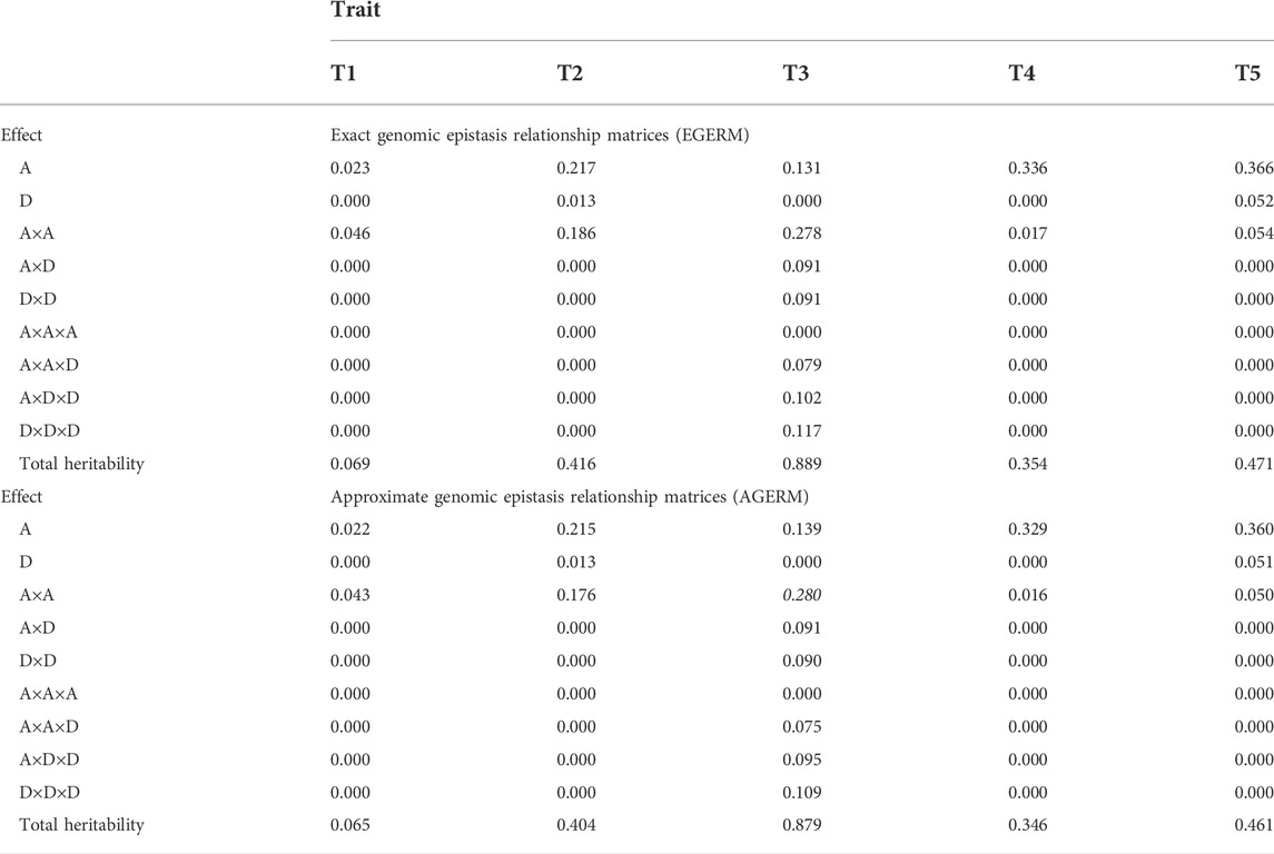
TABLE 1. Genomic heritability estimates of additive, dominance, and epistasis effects up to the third-order for five traits in a swine population.
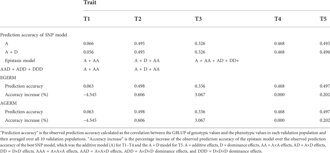
TABLE 2. Observed prediction accuracy of epistasis models relative to the additive model for five traits in a swine population.
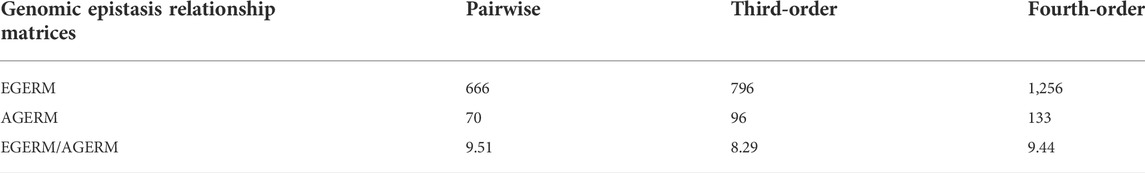
TABLE 3. Computing time (in seconds) for the construction of exact and approximate genomic epistasis relationship matrices for a swine population with 3,534 pigs and 52,843 SNPs using 20 threads of the Mangi supercomputer of the Minnesota Supercomputer Institute at the University of Minnesota.
Numerical demonstration
The methods of genomic epistasis relationship matrices based on the additive and dominance model matrices, GREML, GBLUP and reliability, and estimation of effect heritability are demonstrated using an R program (DEMO.R) and a small artificial sample for the convenience of reading the numerical results (Supplementary Text S2 and R program). Because of the artificial nature and the extremely small sample size, this numerical demonstration does not have any genetic and methodology implications and is for showing calculations of the methods only. This R program is an extension of the R demo program of GVCHAP that integrates SNP and haplotype effects and has a computing pipeline for producing the input haplotype data from the SNP data (Prakapenka et al., 2020).
Conclusion
The multifactorial methods with SNP, haplotype, and epistasis effects up to the third-order provide an approach to investigate the contributions of global low-order and local high-order epistasis effects to the phenotypic variance and the accuracy of genomic prediction. Genomic heritability of each effect type from GREML and prediction accuracy from validation studies using GBLUP can be used jointly to identify effect types contributing to the phenotypic variance and the accuracy of genomic prediction, and the GBLUP for the multifactorial model with selected effect type can be used for genomic evaluation. With many capabilities, including the use of intra- and inter-chromosome separately, the multifactorial methods offer a significant methodology capability to investigate and utilize complex genetic mechanisms for genomic prediction and for understanding the complex genome–phenome relationships.
Data availability statement
Publicly available datasets were analyzed in this study. These data can be found at: https://academic.oup.com/g3journal/article/2/4/429/6026060#supplementary-data.
Author contributions
YD conceived this study and derived the formulations. ZL contributed to formulations of the epistasis genomic relationships, implemented the epistasis methods in EPIHAP, and validated and evaluated the methods. DP contributed to the data processing for methodology evaluation. YD and ZL prepared the manuscript.
Funding
This research was supported by the National Institutes of Health’s National Human Genome Research Institute, grant R01HG012425, as part of the NSF/NIH Enabling Discovery through Genomics (EDGE) Program; grant 2020-67015-31133 from the USDA National Institute of Food and Agriculture; and project MIN-16-124 of the Agricultural Experiment Station at the University of Minnesota. The funders had no role in study design, data collection and analysis, decision to publish, or preparation of the manuscript. The use of the Ceres and Atlas computers in this research was supported by USDA-ARS projects 8042-31000-002-00-D and 8042-31000-001-00-D.
Acknowledgments
The supercomputer of Minnesota Supercomputer Institute at the University of Minnesota and the Ceres and Atlas high-performance computing system of USDA-ARS were used for the evaluation and testing of the methods and EPIHAP computing package. The authors thank Paul VanRaden, Steven Schroeder, and Ransom Baldwin for help with the use of the USDA-ARS computing facilities.
Conflict of interest
The authors declare that the research was conducted in the absence of any commercial or financial relationships that could be construed as a potential conflict of interest.
Publisher’s note
All claims expressed in this article are solely those of the authors and do not necessarily represent those of their affiliated organizations, or those of the publisher, the editors, and the reviewers. Any product that may be evaluated in this article, or claim that may be made by its manufacturer, is not guaranteed or endorsed by the publisher.
Supplementary material
The Supplementary Material for this article can be found online at: https://www.frontiersin.org/articles/10.3389/fgene.2022.922369/full#supplementary-material
References
Bian, C., Prakapenka, D., Tan, C., Yang, R., Zhu, D., Guo, X., et al. (2021). Haplotype genomic prediction of phenotypic values based on chromosome distance and gene boundaries using low-coverage sequencing in Duroc pigs. Genet. Sel. Evol. 53 (1), 78–19. doi:10.1186/s12711-021-00661-y
Carlborg, Ö., and Haley, C. S. (2004). Epistasis: Too often neglected in complex trait studies? Nat. Rev. Genet. 5 (8), 618–625. doi:10.1038/nrg1407
Cleveland, M. A., Hickey, J. M., and Forni, S. (2012). A common dataset for genomic analysis of livestock populations. G3 2 (4), 429–435. doi:10.1534/g3.111.001453
Cockerham, C. C. (1954). An extension of the concept of partitioning hereditary variance for analysis of covariances among relatives when epistasis is present. Genetics 39 (6), 859–882. doi:10.1093/genetics/39.6.859
Cordell, H. J. (2002). Epistasis: What it means, what it doesn't mean, and statistical methods to detect it in humans. Hum. Mol. Genet. 11 (20), 2463–2468. doi:10.1093/hmg/11.20.2463
Da, Y. (2015). Multi-allelic haplotype model based on genetic partition for genomic prediction and variance component estimation using SNP markers. BMC Genet. 16 (1), 144. doi:10.1186/s12863-015-0301-1
Da, Y., Tan, C., and Parakapenka, D. (2016). 0336 Joint SNP-haplotype analysis for genomic selection based on the invariance property of GBLUP and GREML to duplicate SNPs. J. Animal Sci. 94 (5), 161–162. doi:10.2527/jam2016-0336
Da, Y., Wang, C., Wang, S., and Hu, G. (2014). Mixed model methods for genomic prediction and variance component estimation of additive and dominance effects using SNP markers. PLoS One 9 (1), e87666. doi:10.1371/journal.pone.0087666
Hayes, B., and Goddard, M. (2010). Genome-wide association and genomic selection in animal breeding. Genome 53 (11), 876–883. doi:10.1139/G10-076
Henderson, C. (1977). Best linear unbiased prediction of breeding values not in the model for records. J. Dairy Sci. 60 (5), 783–787. doi:10.3168/jds.s0022-0302(77)83935-0
Henderson, C. (1985). Best linear unbiased prediction of nonadditive genetic merits in noninbred populations. J. Animal Sci. 60 (1), 111–117. doi:10.2527/jas1985.601111x
Jiang, Y., and Reif, J. C. (2020). Efficient algorithms for calculating epistatic genomic relationship matrices. Genetics 216 (3), 651–669. doi:10.1534/genetics.120.303459
Jiang, Y., and Reif, J. C. (2015). Modeling epistasis in genomic selection. Genetics 201 (2), 759–768. doi:10.1534/genetics.115.177907
Johnson, D., and Thompson, R. (1995). Restricted maximum likelihood estimation of variance components for univariate animal models using sparse matrix techniques and average information. J. Dairy Sci. 78 (2), 449–456. doi:10.3168/jds.s0022-0302(95)76654-1
Kempthorne, O. (1954). The correlation between relatives in a random mating population. Proc. R. Soc. Lond. B Biol. Sci. 143 (910), 102–113.
Lee, S. H., and van der Werf, J. H. (2006). An efficient variance component approach implementing an average information REML suitable for combined LD and linkage mapping with a general complex pedigree. Genet. Sel. Evol. 38 (1), 25–43. doi:10.1186/1297-9686-38-1-25
Liang, Z., Prakapenka, D., and Da, Y. (2022). Comparison of two methods of genomic epistasis relationship matrices using daughter pregnancy rate in U.S. Holstein cattle. Abstract 2466V, page 409 of ADSA2022 Abstracts. Available at: https://www.adsa.org/Portals/0/SiteContent/Docs/Meetings/2022ADSA/Abstracts_BOOK_2022.pdf?v=20220613 (Accessed September 27, 2022).
Liang, Z., Prakapenka, D., and Da, Y. (2021). Epihap: A computing tool for genomic estimation and prediction using global epistasis effects and haplotype effects. Abstract P167, page 223 of ADSA2021 Abstracts, ADSA 2021 Virtual Annual Meeting. Available at: https://www.adsa.org/Portals/0/SiteContent/Docs/Meetings/2021ADSA/ADSA2021_Abstracts.pdf (Accessed September 27, 2022).
Liang, Z., Tan, C., Prakapenka, D., Ma, L., and Da, Y. (2020). Haplotype analysis of genomic prediction using structural and functional genomic information for seven human phenotypes. Front. Genet. 11 (1461), 588907. doi:10.3389/fgene.2020.588907
Mackay, T. F. (2014). Epistasis and quantitative traits: Using model organisms to study gene–gene interactions. Nat. Rev. Genet. 15 (1), 22–33. doi:10.1038/nrg3627
Martini, J. W., Toledo, F. H., and Crossa, J. (2020). On the approximation of interaction effect models by Hadamard powers of the additive genomic relationship. Theor. Popul. Biol. 132, 16–23. doi:10.1016/j.tpb.2020.01.004
Martini, J. W., Wimmer, V., Erbe, M., and Simianer, H. (2016). Epistasis and covariance: How gene interaction translates into genomic relationship. Theor. Appl. Genet. 129 (5), 963–976. doi:10.1007/s00122-016-2675-5
Muñoz, P. R., Resende, M. F., Gezan, S. A., Resende, M. D. V., de los Campos, G., Kirst, M., et al. (2014). Unraveling additive from nonadditive effects using genomic relationship matrices. Genetics 198 (4), 1759–1768. doi:10.1534/genetics.114.171322
Phillips, P. C. (2008). Epistasis—The essential role of gene interactions in the structure and evolution of genetic systems. Nat. Rev. Genet. 9 (11), 855–867. doi:10.1038/nrg2452
Prakapenka, D., Liang, Z., Jiang, J., Ma, L., and Da, Y. (2021). A Large-scale genome-wide association study of epistasis effects of production traits and daughter pregnancy rate in US Holstein cattle. Genes 12 (7), 1089. doi:10.3390/genes12071089
Prakapenka, D., Wang, C., Liang, Z., Bian, C., Tan, C., and Da, Y. (2020). Gvchap: A computing pipeline for genomic prediction and variance component estimation using haplotypes and SNP markers. Front. Genet. 11, 282. doi:10.3389/fgene.2020.00282
Ritchie, M. D., and Van Steen, K. (2018). The search for gene-gene interactions in genome-wide association studies: Challenges in abundance of methods, practical considerations, and biological interpretation. Ann. Transl. Med. 6 (8), 157. doi:10.21037/atm.2018.04.05
Segre, D., DeLuna, A., Church, G. M., and Kishony, R. (2005). Modular epistasis in yeast metabolism. Nat. Genet. 37 (1), 77–83. doi:10.1038/ng1489
Su, G., Christensen, O. F., Ostersen, T., Henryon, M., and Lund, M. S. (2012). Estimating additive and non-additive genetic variances and predicting genetic merits using genome-wide dense single nucleotide polymorphism markers. PloS One 7 (9), e45293. doi:10.1371/journal.pone.0045293
Tan, C., Wu, Z., Ren, J., Huang, Z., Liu, D., He, X., et al. (2017). Genome-wide association study and accuracy of genomic prediction for teat number in Duroc pigs using genotyping-by-sequencing. Genet. Sel. Evol. 49 (1), 35. doi:10.1186/s12711-017-0311-8
VanRaden, P. M. (2008). Efficient methods to compute genomic predictions. J. Dairy Sci. 91 (11), 4414–4423. doi:10.3168/jds.2007-0980
Vitezica, Z. G., Legarra, A., Toro, M. A., and Varona, L. (2017). Orthogonal estimates of variances for additive, dominance, and epistatic effects in populations. Genetics 206 (3), 1297–1307. doi:10.1534/genetics.116.199406
Wang, C., and Da, Y. (2014). Quantitative genetics model as the unifying model for defining genomic relationship and inbreeding coefficient. PLoS One 9 (12), e114484. doi:10.1371/journal.pone.0114484
Keywords: multifactorial model, epistasis, haplotype, SNP, GBLUP, GREML
Citation: Da Y, Liang Z and Prakapenka D (2022) Multifactorial methods integrating haplotype and epistasis effects for genomic estimation and prediction of quantitative traits. Front. Genet. 13:922369. doi: 10.3389/fgene.2022.922369
Received: 17 April 2022; Accepted: 12 September 2022;
Published: 14 October 2022.
Edited by:
Kefei Chen, Curtin University, AustraliaReviewed by:
Tianjing Zhao, University of California, Davis, United StatesJosé Marcelo Soriano Viana, Universidade Federal de Viçosa, Brazil
Copyright © 2022 Da, Liang and Prakapenka. This is an open-access article distributed under the terms of the Creative Commons Attribution License (CC BY). The use, distribution or reproduction in other forums is permitted, provided the original author(s) and the copyright owner(s) are credited and that the original publication in this journal is cited, in accordance with accepted academic practice. No use, distribution or reproduction is permitted which does not comply with these terms.
*Correspondence: Yang Da, eWRhQHVtbi5lZHU=