 Michael Sekula
 Jeremy Gaskins
 Susmita Datta2*
95% of researchers rate our articles as excellent or good
Learn more about the work of our research integrity team to safeguard the quality of each article we publish.
Find out more
METHODS article
Front. Genet. , 04 February 2022
Sec. Computational Genomics
Volume 12 - 2021 | https://doi.org/10.3389/fgene.2021.810816
This article is part of the Research Topic Artificial Intelligence for Extracting Phenotypic Features and Disease Subtyping Applied to Single-Cell Sequencing Data View all 8 articles
Differential network analysis plays an important role in learning how gene interactions change under different biological conditions, and the high resolution of single-cell RNA (scRNA-seq) sequencing provides new opportunities to explore these changing gene-gene interactions. Here, we present a sparse hierarchical Bayesian factor model to identify differences across network structures from different biological conditions in scRNA-seq data. Our methodology utilizes latent factors to impact gene expression values for each cell to help account for zero-inflation, increased cell-to-cell variability, and overdispersion that are unique characteristics of scRNA-seq data. Condition-dependent parameters determine which latent factors are activated in a gene, which allows for not only the calculation of gene-gene co-expression within each group but also the calculation of the co-expression differences between groups. We highlight our methodology’s performance in detecting differential gene-gene associations across groups by analyzing simulated datasets and a SARS-CoV-2 case study dataset.
Gene network modeling has become essential to the understanding of complex biological systems related to health and disease. These networks allow researchers to uncover and interpret relationships and interactions between genes during different biological processes (Blencowe et al., 2019). There are several popular methods for constructing gene networks from microarray and bulk RNA sequencing data (Margolin et al., 2006; Langfelder and Horvath, 2008; Huynh-Thu et al., 2010), and more recently, methods for identifying gene networks from single-cell RNA sequencing (scRNA-seq) data have also been proposed (Specht and Li, 2016; Chan et al., 2017; Matsumoto et al., 2017; Sekula et al., 2020). Interestingly, the vast majority of these methods have focused only on analyzing gene expressions from one cellular population, such as a single tissue type, disease, or environmental condition.
Since biological systems are highly dynamic, there is also great interest in performing differential network analysis to examine the changes in network structure under different biological settings. In the context of bulk population data (i.e., microarray and bulk RNA sequencing), efforts have been made to develop different strategies for identifying differences between gene-gene networks. Some approaches propose qualitative analyses through visual inspection of different network topologies (Caldana et al., 2011; Weston et al., 2011), while others rely on statistical tests to determine differences across conditions (Choi and Kendziorski, 2009; Gill et al., 2010; Fukushima, 2013).
For scRNA-seq data, some research has been focused on providing guidelines and procedures for differential network analysis based on existing methods that have been developed to analyze different types of transcriptome data (e.g., bulk RNA sequencing, microarray). Cui et al. (2021) propose a pipeline for comparing two single-cell clusters that includes differential gene correlation analysis from McKenzie et al. (2016), weighted correlation network analysis from Langfelder and Horvath (2008), and differential network analysis with the method DiffCoEx (Tesson et al., 2010). Wang et al. (2017) present several proof-of-concept analyses of scRNA-seq data to identify genes that are differentially connected across distinct biological conditions by utilizing a differential connectivity test originally developed by Gill et al. (2010) for microarray gene expression data.
Some research has also been focused in developing new methods designed specifically for scRNA-seq data to identify and compare gene networks from two (or more) biological conditions. In Chiu et al. (2018), a differential network analysis method for scRNA-seq data is proposed that first determines a sample size corrected gene-gene correlation matrix for each cellular state and then identifies differential gene-gene pairs across the states. Ye et al. (2020) use co-expression network analysis and subgraph learning to identify interactive gene groups within subpopulations of cells from scRNA-seq data. Both Dai et al. (2019) and Li et al. (2021) propose novel methods to create cell-specific networks to examine the overall associations between genes for each individual cell. From these cell-specific networks, researchers can further identify changes in gene-gene networks across different cellular populations and/or different time points.
In this work, we propose a hierarchical Bayesian factor model for constructing gene co-expression networks (GCNs) from scRNA-seq data to explore differences in the network structure across various cell groups due to different biological conditions, cell types, cell stages, or other group choice. Treatment-dependent parameters in our model determine which latent factors are activated in a gene, thereby allowing for the calculation of gene-gene co-expression within each treatment group. For simplicity, we consider a two-group setting and refer to these groups as treatment and control, but our model can easily be extended to a multiple group scenario, if necessary.
The rest of this manuscript is organized as follows. We define our proposed model and inference for differential network analysis in Section 2. Results from simulation studies and real data analysis are presented in Section 3 to demonstrate the performance of our methodology. In Sections 4 and 5, we conclude with a discussion on our results and findings.
Let Ygi be the expression count of gene g (g = 1, …, G) in cell i (i = 1, …, N) for treatment ti ∈ {0, 1}, where ti = 0 represents that cell i belongs in the control (reference) group and ti = 1 for the treatment group. We assume that each expression comes from the Poisson(μgi) distribution (conditionally) and model the log-mean log(μgi) through the representation
For each cell i, there are F associated latent factors λi = {λi1, …, λiF} that impact the expression. Each factor can be thought of as some unique cellular attribute (e.g., cell stage, pseudotime point) that will only affect a specific set of related gene expressions. Since we are defining our model on the log scale, we assume these factors come from a Normal(0, 1) distribution. Marginally over λi, the parameter βg denotes the log-mean expression for gene g in the control group, and βg + δg is the log-mean expression for gene g in the treatment group. Hence, δg represents the log-fold change in the expression for gene g.
The magnitude of the impact of factor f on gene g in treatment t is influenced by the parameter
For most factors, we assume that the values of αgf;0 and αgf;1 in our model will be similar. That is, we expect αgf;0 and αgf;1 to be similar for most (g, f) pairs. We also expect each factor f to impact only a small number of genes, and so the αt matrices will be sparse. To that end, we define the following hierarchy on the αgf;t parameters:
where half−Cauchy(0, 1) is the standard half-Cauchy distribution with the probability density function
We refer to this model definition as Sparse Factor Model - Single HorseShoe (SFM-SHS). Under this scheme, the horseshoe prior (Carvalho et al., 2009) placed on each αgf;t in Eq. 2 will help shrink the values of αgf;0 and αgf;1 together toward the common value
To achieve more sparsity, a horseshoe prior could also be placed on the
We refer to this second model definition as Sparse Factor Model - Double HorseShoe (SFM-DHS). Here, ζ is a global shrinkage parameter that will pull the values of
The flexibility of our defined factor structure allows for the zero-inflation and high cell-to-cell variability typical of scRNA-seq data. For a given factor f, the latent λif is unique to each cell i and only affects a particular gene within a treatment when αgf;t ≠ 0. If the activated factors λifαgf;t for a given gene are highly negative, then μgi will be very small and account for the high proportion of zeros typical of this data. Conversely, large positive values of the factors will increase μgi (relative to the baseline of either exp{βg} for the control group or exp{βg + δg} for the treatment group) and yield extremely large counts, i.e., overdispersion. In Eq. 1, the adjustment term of
Hence, Ygi is conditionally Poisson but marginally overdispersed.
To complete the specification of our Bayesian model, we define priors for the average gene expression parameters as
This model uses the parameters αgf;t to characterize the relationship between the genes and a set of latent factors; however, our real interest is in using these parameters to learn about the genes themselves (marginally over these factors). While the αt matrices in our model impose a crude network structure on the gene expressions for each treatment, the individual αgf;t parameters are non-identifiable, and so we cannot perform inference about these parameters directly. To that end, we consider the matrices
For a given treatment t, the (g, g′) element (g ≠ g′) of the G × G matrix At provides a summation of impact by the associated factors that are active in both genes g and g′ since
With the marginal variance for log(μgi) being
the correlation between log(μgi) and log(μg′i) is defined as
We focus our interest on the marginal correlation of the log-means due to the simplistic nature of the correlation structure and its reliance on only the αgf;t parameters. As displayed in Eq. 5, the variance expression of Ygi includes a set of βg and δg parameters that cannot be factored out, which means the correlation structure between Ygi and Yg′i will depend on the average expression for each gene in each treatment. For this reason, we do not utilize the correlation structure between Ygi and Yg′i.
Our methodology is coded in Stan (Stan Development Team, 2020), and the usual approach to Bayesian inference in Stan is to generate samples from the posterior distributions with Hamiltonian Monte Carlo (HMC; Neal, 2011). The estimated gene-gene network structure
When performing differential network analysis, the interest is in examining the difference between ρgg′;0 and ρgg′;1 (θgg′ = ρgg′;0 − ρgg′;1), and both the posterior mean
We note that an iterative Markov Chain Monte Carlo (MCMC) approach may be computationally intensive for larger scRNA-seq datasets and will require the user to perform various diagnostic checks to ensure MCMC convergence and mixing (Cowles and Carlin, 1996). For those reasons, we present an alternative strategy for inference of our model parameters. A posterior mode estimate from our model can be obtained by maximizing the joint posterior via the optimizing function from Stan. With this optimized estimate, we calculate the marginal correlation structure from each treatment group defined in Eq. 6 and determine each gene-gene pair correlation difference
To produce an estimate of variability for θgg′, we utilize a nonparametric bootstrap procedure. For each bootstrap iteration (mb) we perform the following:
1) Resample the cellular data with replacement within each treatment group. Here, the number of cells within each treatment group remains the same, but a new sample of cellular data for each treatment group is randomly selected from the original treatment group data.
2) Obtain a posterior mode estimate from the resampled data with the optimizing function from Stan.
3) Determine the marginal correlation structure as defined in Eq. 6 for each treatment and then calculate
From the Mb total bootstrap samples, a 100(1 − α∗)% confidence interval (CI) can be created and analyzed for ρgg′;0, ρgg′;1, and θgg′ in the same manner as previously described above for the posterior CrIs. Figure 1 displays a flowchart of our proposed methodology. We note that we describe three estimation approaches/algorithms for our methodology, each with varying levels of computational complexity. The nonparametric bootstrap procedure is our preferred approach as will be shown in Section 3.
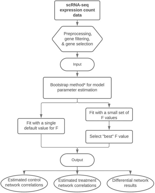
FIGURE 1. Flowchart of our proposed methodology to perform differential network analysis from scRNA-seq data. The input is a preprocessed scRNA-seq dataset and the output consists of the estimated control and treatment gene-gene correlations and the differential network with significant gene-gene differences between treatment groups. *Note: The bootstrap method is our recommended technique for model parameter estimation, but parameter estimation could alternatively be performed with a single posterior optimization or via HMC.
To evaluate the performance of our methodology, we simulated count data from marginal zero-inflated negative binomial distributions via the NORmal To Anything (NORTA) algorithm (Cario and Nelson, 1997). The NORTA algorithm generates a random vector from a multivariate standard normal distribution with a given correlation structure and transforms it into a random vector with a specified marginal distribution. Counts were generated with the rnorta function from the R package SimCorMultRes (Touloumis, 2016), and the ZIM package (Yang et al., 2018) was used to estimate the parameters of the zero-inflated negative binomial distributions from genes randomly selected from the genes considered in a previous analysis (Sekula et al., 2020) of the mouse microglia cell data from Tay et al. (2018). It is important to emphasize that the simulated data come from a different generating model than our proposed estimation approach.
We considered four different simulation schemes to create datasets of different sizes, using either G = 50 or G = 100 genes and setting the total number of cells to either N = 500, N = 1, 000, or N = 2, 000 (see Table 1 for details of each simulation scheme). To define treatment groups, the cells were divided equally into the control group (t = 0) and the treatment group (t = 1). Correlation structures for each treatment network were fixed to create a differential structure of 325 different edges with G = 50 genes (Sim 1, Sim 2, and Sim 3) and 1,300 different edges with G = 100 genes (Sim 4).
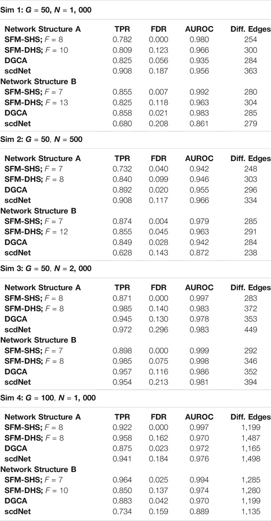
TABLE 1. Comparison of the “true” differences between networks and the estimated differences between networks in the simulation studies for each differential network method. Results displayed for SFM-SHS and SFM-DHS are from the bootstrap estimation procedure. In Sim 1–3, there are 325 “true” differential edges and in Sim 4 there are 1, 300 “true” differential edges.
In our simulation data, we control the correlation structures by sorting genes into ten equal groups (e.g., Group 1 consisted of the first set of G/10 genes, Group 2 consisted of the second set of G/10 genes). Genes within the same group are defined to be highly correlated and share correlation structures across the other gene groups. Two different sets of correlation structures (Network Structure A and Network Structure B) were utilized for each simulation scheme, and the magnitudes of the “true” differences between correlations (θgg′ = ρgg′;0 − ρgg′;1) ranged from 0.27 to 1.43 as displayed in Figure 2. For Network Structure B, some of the gene-gene pairs were simulated to have opposite correlation directions in each treatment group, thereby creating larger correlation differences between the groups.
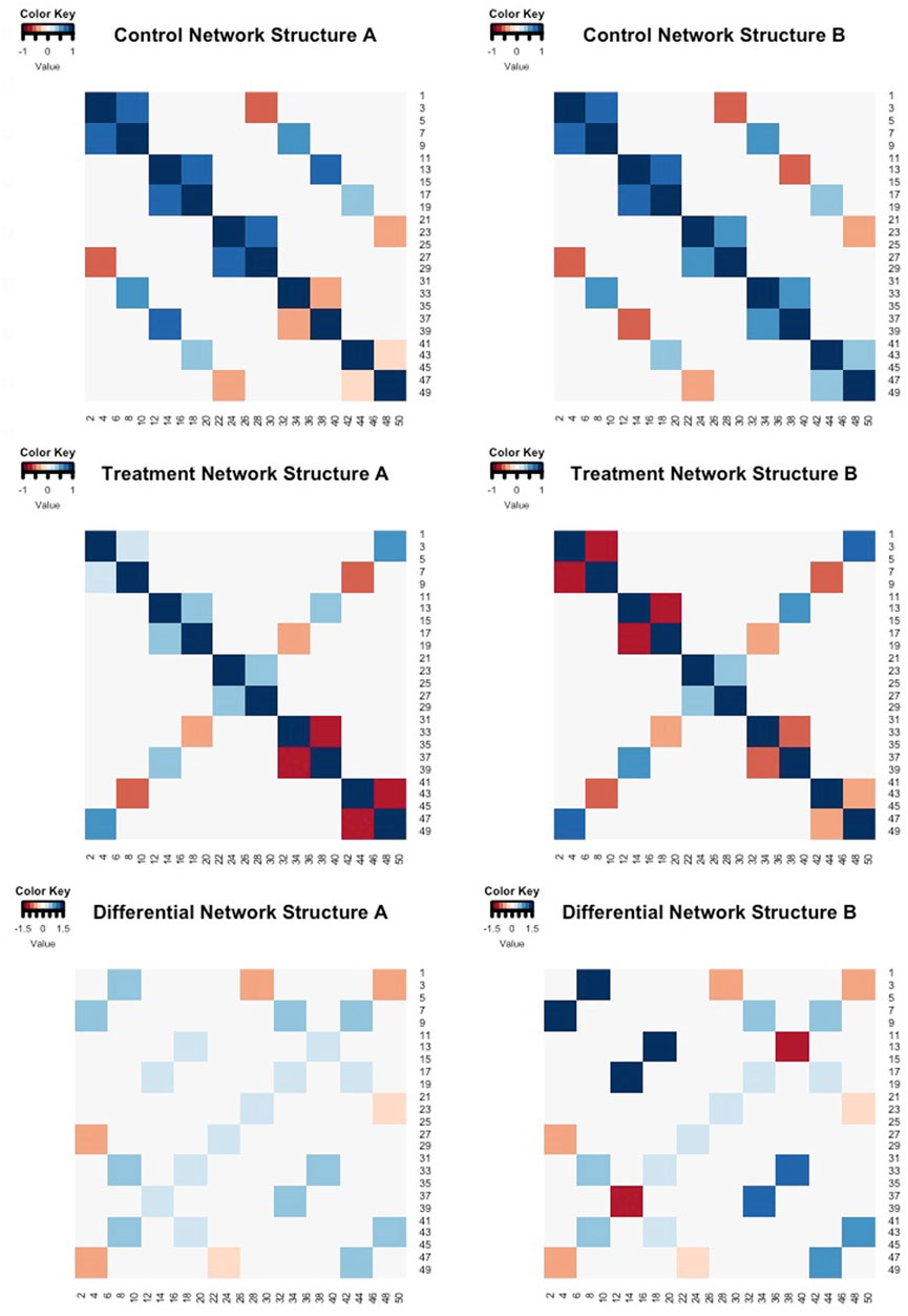
FIGURE 2. Heatmaps of the “true” correlation structures of control group (row 1) and treatment group (row 2) for Network Structure A and Network Structure B. The colored cells in these heatmaps represent the magnitude and direction of gene-gene correlations. Row 3 contains the differences between the control and treatment correlation structures. The colored cells in row 3 indicate the magnitude and direction of the differences in gene-gene associations across the two groups (control - treatment).
Two versions of our sparse Bayesian factor methodology were investigated in the simulation studies. In our first model version SFM-SHS, the priors defined in Eqs. 2, 3 are placed on the αgf;t and
Using the simulated data, we ran our proposed models in R (R Core Team, 2018) interfacing with Stan through the package rstan (Stan Development Team, 2020). Here, we utilize the bootstrap procedure for parameter estimation and inference was performed on 1,000 bootstrap samples. To investigate whether the number of factors (F) makes any impact on model performance, we ran both models multiple times and input a different number of factors for each run, starting with F = 5 and increasing the number of factors up until F = 20. From our simulation studies, we found that area under the receiver operating characteristic curve (AUROC) for the performance of our models is relatively consistent with choices of F that are greater than 5, see Table 2. The inverse of the approximate “p-value” (defined in Section 2.3) for each
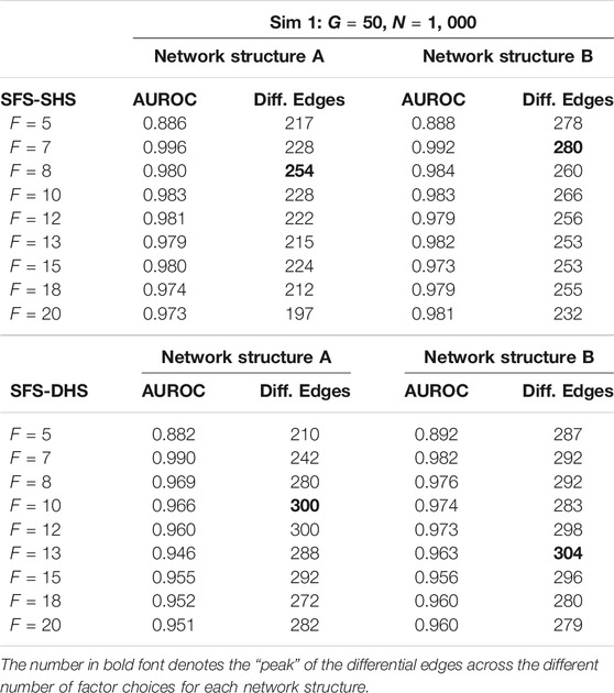
TABLE 2. Example comparisons of AUROC and number of significant differential edges (Diff. Edges) from Sim 1 when different choices of F are input into the SFM-SHS and SFM-DHS methods. Results are presented from the bootstrap estimation procedure.
To identify an appropriate choice for the tuning parameter F, the number of factors in our model, we examined the number of significant differential network edges. In Figure 3, we plotted the proportion of differential network edges (number of differential network edges divided by
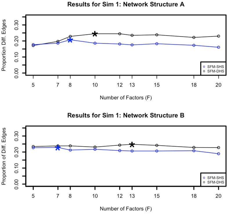
FIGURE 3. Example proportions of significant differential network edges (number of significant differential network edges divided by
For the simulation studies, we ran also analyses with two other differential network methods that detect differences based on correlation structures between groups. One of the competitor methods we considered was Differential Gene Correlation Analysis (DGCA; McKenzie et al., 2016), which is an R package developed for identifying differential correlations between gene pairs in various types of genomic data (microarray, bulk RNA-seq, scRNA-seq, etc.). DGCA transforms correlation coefficients to z-scores and uses differences in z-scores to generate empirical p-values for the differential correlation between genes. These empirical p-values are then used to calculate q-values for an FDR threshold, and a q-value of 0.05 was set to denote significant differences for this method.
The other method considered in our simulated studies was scRNA-seq-based differential network analysis (scdNet), which is a differential network method developed specifically for scRNA-seq data by Chiu et al. (2018). In scdNet, a sample size adjustment transformation is first applied to the correlation coefficients within each cellular group and then statistical inference is performed on the differences in the transformed correlations across groups. The scdNet method provides p-values to represent differential results for each gene-gene pair, and we controlled the FDR with the Benjamini and Hochberg (1995) procedure. A threshold of 5% was used to indicate significant differences with scdNet.
For each simulated dataset, we compared the significant differences between networks that were identified by each method (SFM-SHS, SFM-DHS, DGCA, and scdNet) to the “true” differences between networks. The measures of TPR, FDR, AUROC, and the number of edges that were classified as significantly different between networks by each method are displayed in Table 1. From this table, we see that our differential network methodology performs quite well compared to the competitor methods of DGCA and scdNet. Both SFM-SHS and SFM-DHS have high TPRs and AUROCs while also controlling the FDRs to a nominal rate. In general, SFM-SHS tends to be a bit more conservative and detects fewer significant edges than SFM-DHS, but SFM-SHS performs better at controlling FDRs below a threshold of 5%. In fact, SFM-SHS was the only method out of the four to consistently control the FDR to a nominal rate across the simulation cases, while scdNet tends to have the highest FDR. The AUROCs for both SFM-SHS and SFM-DHS are also comparable or better than the AUROCs by DGCA and scdNet across most simulations.
To demonstrate the utility of bootstrap estimation compared to the other parameter estimation techniques discussed in Section 2.3, we performed a secondary analysis comparing the results of our methods from bootstrapping to the results of our methods generated by a single optimization and by a full HMC sampler. For the single optimization technique (i.e., finding the posterior mode), the significance of each difference cannot be directly determined; therefore, we identified the Top 10% of edges with the largest difference between treatment groups and calculated the AUROC with the magnitudes (absolute values) of the estimated correlation differences. For the full HMC, we utilized rstan and combined results from 4 separate chains, with each chain running 1,000 warmup iterations and 1,000 sampling iterations for a total of 4,000 samples. Due to the slow speed of HMC sampling, only the results from the smallest simulated datasets (Sim 2: G = 50 genes and N = 500 cells) are presented.
The results in Table 3 highlight the benefits of using optimization and bootstrapping. Both the full HMC sampler and the bootstrap technique obtain high TPRs and AUROCs, but the HMC sampler tends to have higher FDRs and also has very long computational times. The single optimization technique is also able to achieve high AUROC simply by ranking the magnitudes of the correlation differences between groups. Thus, a single optimization could be useful as a method to quickly identify highly differential edges between networks. We note that bootstrap optimizations can be run simultaneously in parallel and by increasing the number of available cores, the computational efficiency of the bootstrap technique will be increased.
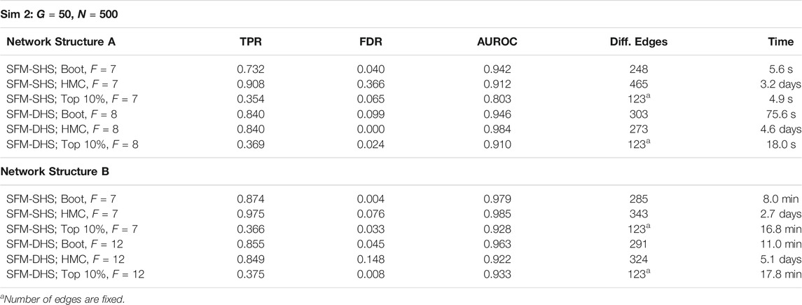
TABLE 3. Results for SFM-SHS and SFM-DHS when utilizing bootstrap (Boot), HMC, and the Top 10% of differential edges from a single optimization. Times for Boot represent the average time of one posterior optimization of a single resampled dataset; similarly, HMC time is the average time for a single MCMC chain.
To further examine our proposed methodology, we analyzed the real dataset from Bacher et al. (2020), which consists of scRNA-seq expressions derived from SARS-CoV-2-reactive memory T cells. This data was obtained from the Gene Expression Omnibus (GEO) database under accession number GSE162086. We examined 1,833 cells that were identified by Bacher et al. (2020) as cells with distinct transcriptional profiles related to cytotoxic-Th1 and cycling. These cells are divided into two patient groups: N0 = 462 cells are from non-hospitalized patients with SARS-CoV-2 and the remaining N1 = 1, 371 cells come from patients hospitalized with SARS-CoV-2. After filtering out genes that were not expressed in at least 20% of the cells, we used the R package MAST (Finak et al., 2015) to identify G = 130 differentially expressed genes with a log2 fold change (as estimated by MAST) of at least log 2(1.2) for further analysis.
For each method considered in Section 3.1, we conducted a differential network analysis and ranked each gene by the number of significant differential connections. SFM-SHS and SFM-DHS were implemented with the bootstrapping estimation approach, and we selected the “best” model choice by identifying the “peak” in the number of differential edges starting with F = 5 factors and increasing the number of factors up to F = 20. The UpSet plot (Lex et al., 2014) for the intersection between the differential edges detected by each method is displayed in Figure 4. The dark circles in each column of the UpSet plot indicate the methods associated with the intersection and the bar above each column represents the number of differential edges in the intersection.
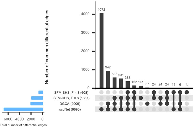
FIGURE 4. UpSet plot of the number of differential edges determined by four differential network methods in the SARS-CoV-2 case study dataset. The numbers in parentheses represent the total number of differential edges detected by the corresponding method. Results displayed for SFM-SHS and SFM-DHS are from the bootstrap estimation procedure.
From Figure 4, we see that the methods performed quite differently as only 388 edges were common across all four methods. SFM-SHS was the most conservative method and detected 608 differential edges, while scdNet method detected 6,690 differential edges, which is nearly 80% of the 8,385 total number of possible edges. Because the differential network analyses from the methods were so different, we selected the top genes with the most gene-gene pair connections from each method and used those top differentially connected genes (DCGs) to evaluate the performance of the methods in this case study analysis. A total of 14 DCGs (approximately 10% of the G = 130 total genes) were identified from each of the SFM-SHS, SFM-DHS, and DGCA analyses. From the scdNet analysis, 15 DCGs were chosen because three genes tied for the 13th, 14th, and 15th ranks.
In Figure 5, the UpSet plot for the intersection between the top DCGs detected by each differential network method is displayed. Here, the bar above each column in the figure represents the number of DCGs in the intersection. Interestingly, there was not much overlap in the top DCGs detected by the methods considered in this analysis. Our methods (SFM-SHS, SFM-DHS) detect seven unique DCGs from the other methods, whereas DGCA and scdNet identified six and nine unique DCGs, respectively.
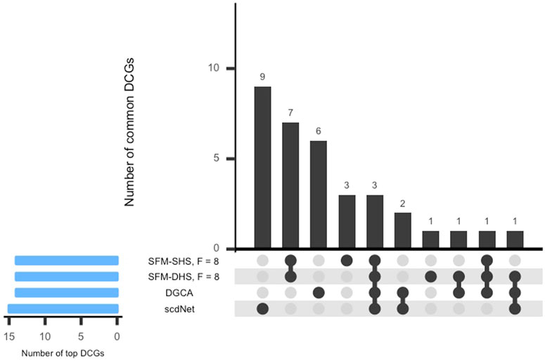
FIGURE 5. UpSet plot of the top DCGs determined by four differential network methods in the SARS-CoV-2 case study dataset. Results displayed for SFM-SHS and SFM-DHS are from the bootstrap estimation procedure.
Only three genes (RPS26, RGCC, RPL3) were common among the top DCGs selected by each method. These three genes play an important role in any immune-related disorders. RPS26 and RPL3 are ribosomal proteins (RP) and both are related to influenza viral RNA transcription and replication. RPs are needed for protein biosynthesis of viruses controlling replication, regulation, and infection inside the host cells. However, a small percentage of these proteins trigger the immune pathway against viruses and protect the host cells. Hence, RPs are now being considered for potential therapeutics for SARS-CoV-2 or any such viral infections (Rofeal and El-Malek, 2020).
To evaluate the biological relevancy of the top DCGs from each method, clusters of gene ontology (GO) categories were created with the functional annotation clustering tool from the database for Annotation, Visualization, and Integrated Discovery (DAVID; Huang et al., 2009a; Huang et al., 2009b). An enrichment score is calculated by DAVID for each cluster to help identify clusters that are involved in more enriched (important) biological roles. As it has been suggested that more attention should be given to groups with enrichment scores greater of 1.3 or higher (Huang et al., 2009b), we used a score threshold of 1.3 to classify clusters as enriched.
SFM-SHS had two enriched clusters from the DAVID functional annotation clustering analysis, while the three other methods (SFM-DHS, DGCA, and scdNet) had just one enriched cluster. SFM-DHS had the cluster with the highest Enrichment Score (3.46), and the top GO terms associated this cluster include SRP-dependent cotranslational protein targeting to membrane, viral transcription, and nuclear-transcribed mRNA catabolic process, nonsense-mediated decay. These same GO terms also appear in the most highly enriched cluster from each of the other three methods, and the corresponding Enrichment Scores from the SFM-SHS, scdNet, and DGCA clusters are 2.95, 2.94, and 2.80, respectively. The DCGs identified by SFM-SHS were also associated with a second enriched cluster. The terms of cytosol, cytoplasm, and phosphoprotein were clustered together with an Enrichment Score of 1.71. All results from DAVID functional annotation clustering tool are provided in the Supplementary Materials.
Lastly, we visualized the differential networks estimated from SFM-SHS and SFM-DHS in Figures 6, 7, respectively. The gene-gene connections in the figures represent the differential edges for the 7 top DCGs uniquely identified by our methods and the 3 top DCGs identified by all four considered methods. All G = 130 genes are displayed in each figure, but we only display the differential edges for the 10 selected DCGs. Figures of the individual GCNs with these 10 DCGs for the non-hospitalized and hospitalized groups are provided in the Supplementary Figures S1–S4.
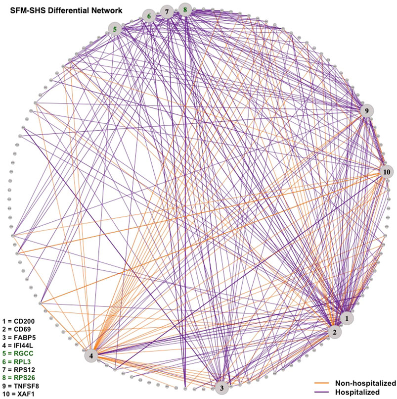
FIGURE 6. Differential network estimated by SFM-SHS with the bootstrap procedure for the SARS-CoV-2 case study dataset. Edges displayed are for 10 DCGs. The 7 unique top DCGs identified by both SFM-SHS and SFM-DHS are listed in black and the 3 top DCGs identified by all considered methods are listed in green. Each edge color represents the group with the larger correlation magnitude.

FIGURE 7. Differential network estimated by SFM-DHS with the bootstrap procedure for the SARS-CoV-2 case study dataset. Edges displayed are for 10 DCGs. The 7 unique top DCGs identified by both SFM-SHS and SFM-DHS are listed in black and the 3 top DCGs identified by all considered methods are listed in green. Each edge color represents the group with the larger correlation magnitude.
We see that a majority of these DCGs have differential edges that are a result of larger correlations in the hospitalized group, with CD200 and TNFSF8 having the highest numbers of differential edges from this group. CD200 is a type 1 cell membrane glycoprotein (GP) of the immunoglobulin supergene family that is expressed by many cell types (e.g., B cells, a subset of T cells, endothelial cells, cancer cells). GP plays an important role in immunosuppression and regulation of anti-tumor activity. Moreover, this gene has multiple transcript variances. Naturally, its connectivities are different in the hospitalized group of patients compared to non-hospitalized group.
TNFSF8 is one of the tumor necrosis factor (TNF) receptor superfamily proteins that typically are composed of one to four cysteine-rich domains. It has been suggested that SARS-CoV-2 disease processes present in severe illness contribute to impaired adaptive immune responses. Additionally, TNF super family proteins are most often used in predicting neutralization. Elderly patients severely affected by SARS-CoV-2 have distinctive neutralization activity-associated protein profiles that may display an altered level of TNFSF8 (Filbin et al., 2021).
Conversely, both IFI44L and XAF1 had the highest number of differential edges as a result of having stronger correlations in the non-hospitalized group. Prior studies concluded that SARS-CoV-2 and other viruses elicit an interferon response in the upper airway. Moreover, the most significant genes upregulated by SARS-CoV-2 were interferon inducible, such as IFI44L (Butler et al., 2021; Huang et al., 2021). XAF1 is an X-linked inhibitor of apoptosis (XIAP)-associated factor 1. This gene participates in pro-apoptotic responses and has multiple transcript variants. In Zhu et al. (2020), both IFI44L and XAF1 were upregulated in T, B, natural killer, and DC cell subsets of SARS-CoV-2 patients compared to healthy controls.
Our proposed model includes continuous treatment-dependent parameters that determine the impact of latent factors for each gene. For simplicity, our methodology has been defined and examined under a two-group situation, but it can be adjusted to a multiple group scenario. In the general case, we can consider T number of treatments and represent the log(μgi) from Eq. 1 in the general form:
Here, the δg;t parameters depend on the treatment groups t ∈ {1, …, T − 1} and I(ti = t) is the indicator variable for cell i being in treatment group t. The construction of gene-gene correlation structures will remain the same, but there will be T sets of αgf;t parameters that create T different networks to compare. When performing differential network analysis, one can examine the CrIs (or CIs) of the difference between ρgg′;t and ρgg′;t′ for each pair of treatments t and t′ (t ≠ t′).
In addition to identifying differential network edges, our methodology also reports estimates of the GCNs for both the control and treatment group. We found that these estimates generally reflect the “true” underlying correlation structures of the simulated datasets used in Section 3.1 (see Supplementary Tables S1, S2). To the best of our knowledge, the method of scdNet currently does not directly provide the estimations of the control and treatment GCNs, separately.
When applying our methodology, we recommend using an optimization-based procedure for estimating model parameters. Researchers can choose to utilize a single optimization of our model and select the “Top N” gene-gene correlation differences from the posterior mode or choose to utilize bootstrapping to obtain and analyze the variability of the estimates. Both techniques achieved high AUROCs in the simulation studies, and the bootstrap optimization was able to control the FDRs. Furthermore, bootstrap replicates can be performed in parallel to help reduce computational time. One could choose to utilize a full HMC to obtain parameter estimates and perform model inference, but an iterative MCMC approach may be computationally expensive and will also require the use of diagnostic tools to assess convergence. As an alternative approach to faster Bayesian computing, we had considered utilizing variational inference as a tool to approximate the posterior distribution and obtain parameter estimates as in Sekula et al. (2019), but our preliminary experiments found that this inference technique did not produce reliable estimates.
When it comes to choosing an appropriate number of factors (F) for our methodology, we recommend running different choices for F and identifying the “peak” in the number of differential network edges after F = 5 factors (as illustrated in Figure 3). Starting with the choice of F = 5 helps to capture the increase in the number of differential edges across increasing values of F, and the number of factors associated with the “peak” can be considered the “best” model choice. Generally, we found that F = 7 or F = 8 for the number of factors was a common selection for both SFM-SHS and SFM-DHS in our considered datasets that had between G = 50 to G = 130 genes. Thus, using either F = 7 or F = 8 would be a reasonable default choice for analyses with similar numbers of genes. For analyses with much larger values of G, one may anticipate needing a larger value for F.
In this manuscript, we have presented a sparse hierarchical Bayesian factor model to perform differential network analysis from scRNA-seq count data. With a latent factor structure, we define a count model that is conditionally Poisson but marginally overdispersed, and the flexibility of the defined latent factor structure allows our model to account for other unique features of scRNA-seq data such as zero-inflation and high cell-to-cell variability. Furthermore, the defined horseshoe prior structures in Eqs. 2–4 promote sparsity in our network estimation and allow information to be shared across treatment groups.
When applying our methodology, our main recommendation is to perform analysis using the SHS version of our model with bootstrapping, as SFM-SHS tends to be better at controlling the FDRs compared to SFM-DHS. We also recommend using some sort of gene selection method (e.g., differential expression) to obtain a manageable number of genes to analyze with our method. Since each GCN is determined by a quadratic number of parameters (
As demonstrated in Section 3.1, the bootstrapping technique for parameter estimation provides a time-efficient implementation of our methodology that outperforms the competitor methods of scdNet and DGCA. Also, our methods were superior in selecting top DCGs that were associated with biologically enriched clusters of GO categories in Section 3.2. Both SFM-SHS and SFM-DHS identified a unique set of top DCGs with biological functions related to the body’s response to the SARS-CoV-2 virus. Collectively, these analyses suggest that our sparse Bayesian factor model will be a useful tool for the construction and differential analysis of GCNs in future scRNA-seq experiments. An R package implementing our proposed methodology and code to generate the simulated datasets are available at: https://github.com/mnsekula/scSFMnet.
Publicly available datasets were analyzed in this study. This data can be found here: https://www.ncbi.nlm.nih.gov/geo/query/acc.cgi?acc=GSE162086.
MS, JG, and SD developed the methodology. MS performed the data analysis and maintains the associated R package. All authors contributed to writing and revising the manuscript and approved the submitted version.
The authors declare that the research was conducted in the absence of any commercial or financial relationships that could be construed as a potential conflict of interest.
All claims expressed in this article are solely those of the authors and do not necessarily represent those of their affiliated organizations, or those of the publisher, the editors and the reviewers. Any product that may be evaluated in this article, or claim that may be made by its manufacturer, is not guaranteed or endorsed by the publisher.
The Supplementary Material for this article can be found online at: https://www.frontiersin.org/articles/10.3389/fgene.2021.810816/full#supplementary-material
Bacher, P., Rosati, E., Esser, D., Martini, G. R., Saggau, C., Schiminsky, E., et al. (2020). Low-avidity CD4+ T Cell Responses to SARS-CoV-2 in Unexposed Individuals and Humans with Severe COVID-19. Immunity 53, 1258–1271. doi:10.1016/j.immuni.2020.11.016
Benjamini, Y., and Hochberg, Y. (1995). Controlling the False Discovery Rate: A Practical and Powerful Approach to Multiple Testing. J. R. Stat. Soc. Ser. B (Methodological) 57, 289–300. doi:10.1111/j.2517-6161.1995.tb02031.x
Blencowe, M., Arneson, D., Ding, J., Chen, Y.-W., Saleem, Z., and Yang, X. (2019). Network Modeling of Single-Cell Omics Data: Challenges, Opportunities, and Progresses. Emerging Top. Life Sci. 3, 379–398. doi:10.1042/ETLS20180176
Butler, D., Mozsary, C., Meydan, C., Foox, J., Rosiene, J., Shaiber, A., et al. (2021). Shotgun Transcriptome, Spatial Omics, and Isothermal Profiling of SARS-CoV-2 Infection Reveals Unique Host Responses, Viral Diversification, and Drug Interactions. Nat. Commun. 12, 1660. doi:10.1101/2020.04.20.048066
Caldana, C., Degenkolbe, T., Cuadros-Inostroza, A., Klie, S., Sulpice, R., Leisse, A., et al. (2011). High-density Kinetic Analysis of the Metabolomic and Transcriptomic Response of Arabidopsis to Eight Environmental Conditions. Plant J. 67, 869–884. doi:10.1111/j.1365-313x.2011.04640.x
Cario, M. C., and Nelson, B. L. (1997). Modeling and Generating Random Vectors with Arbitrary Marginal Distributions and Correlation Matrix. Technical report. Evanston, Illinois: Department of Industrial Engineering and Management Sciences, Northwestern University.
Carvalho, C. M., Polson, N. G., and Scott, J. G. (2009). “Handling Sparsity via the Horseshoe,” in Artificial Intelligence and Statistics. Clearwater Beach, FL: PMLR, 73–80.
Chan, T. E., Stumpf, M. P. H., and Babtie, A. C. (2017). Gene Regulatory Network Inference from Single-Cell Data Using Multivariate Information Measures. Cel Syst. 5, 251–267. doi:10.1016/j.cels.2017.08.014
Chiu, Y.-C., Hsiao, T.-H., Wang, L.-J., Chen, Y., and Shao, Y.-H. J. (2018). scdNet: A Computational Tool for Single-Cell Differential Network Analysis. BMC Syst. Biol. 12, 124. doi:10.1186/s12918-018-0652-0
Choi, Y., and Kendziorski, C. (2009). Statistical Methods for Gene Set Co-expression Analysis. Bioinformatics 25, 2780–2786. doi:10.1093/bioinformatics/btp502
Cowles, M. K., and Carlin, B. P. (1996). Markov Chain Monte Carlo Convergence Diagnostics: A Comparative Review. J. Am. Stat. Assoc. 91, 883–904. doi:10.1080/01621459.1996.10476956
Cui, L., Wang, B., Ren, C., Wang, A., An, H., and Liang, W. (2021). A Novel Method to Identify the Differences between Two Single Cell Groups at Single Gene, Gene Pair, and Gene Module Levels. Front. Genet. 12, 297. doi:10.3389/fgene.2021.648898
Dai, H., Li, L., Zeng, T., and Chen, L. (2019). Cell-specific Network Constructed by Single-Cell RNA Sequencing Data. Nucleic Acids Res. 47, e62. doi:10.1093/nar/gkz172
Filbin, M. R., Mehta, A., Schneider, A. M., Kays, K. R., Guess, J. R., Gentili, M., et al. (2021). Longitudinal Proteomic Analysis of Severe COVID-19 Reveals Survival-Associated Signatures, Tissue-specific Cell Death, and Cell-Cell Interactions. Cel Rep. Med. 2, 100287. doi:10.1016/j.xcrm.2021.100287
Finak, G., McDavid, A., Yajima, M., Deng, J., Gersuk, V., Shalek, A. K., et al. (2015). Mast: A Flexible Statistical Framework for Assessing Transcriptional Changes and Characterizing Heterogeneity in Single-Cell RNA Sequencing Data. Genome Biol. 16, 278. doi:10.1186/s13059-015-0844-5
Fukushima, A. (2013). DiffCorr: An R Package to Analyze and Visualize Differential Correlations in Biological Networks. Gene 518, 209–214. doi:10.1016/j.gene.2012.11.028
Gill, R., Datta, S., and Datta, S. (2010). A Statistical Framework for Differential Network Analysis from Microarray Data. BMC Bioinformatics 11, 95. doi:10.1186/1471-2105-11-95
Huang, D. W., Sherman, B. T., and Lempicki, R. A. (2009a). Bioinformatics Enrichment Tools: Paths toward the Comprehensive Functional Analysis of Large Gene Lists. Nucleic Acids Res. 37, 1–13. doi:10.1093/nar/gkn923
Huang, D. W., Sherman, B. T., and Lempicki, R. A. (2009b). Systematic and Integrative Analysis of Large Gene Lists Using DAVID Bioinformatics Resources. Nat. Protoc. 4, 44–57. doi:10.1038/nprot.2008.211
Huang, L., Shi, Y., Gong, B., Jiang, L., Zhang, Z., Liu, X., et al. (2021). Dynamic blood single-cell immune responses in patients with COVID-19. Sig. Transduct. Target Ther. 6, 110. doi:10.1038/s41392-021-00526-2
Huynh-Thu, V. A., Irrthum, A., Wehenkel, L., and Geurts, P. (2010). Inferring Regulatory Networks from Expression Data Using Tree-Based Methods. PLoS One 5, e12776. doi:10.1371/journal.pone.0012776
Langfelder, P., and Horvath, S. (2008). WGCNA: An R Package for Weighted Correlation Network Analysis. BMC Bioinformatics 9, 559. doi:10.1186/1471-2105-9-559
Lex, A., Gehlenborg, N., Strobelt, H., Vuillemot, R., and Pfister, H. (2014). UpSet: Visualization of Intersecting Sets. IEEE Trans. Vis. Comput. Graph 20, 1983–1992. doi:10.1109/TVCG.2014.2346248
Li, L., Dai, H., Fang, Z., and Chen, L. (2021). c-CSN: Single-Cell RNA Sequencing Data Analysis by Conditional Cell-specific Network. Genomics, Proteomics & Bioinformatics 21, 319–329. doi:10.1016/j.gpb.2020.05.005
Margolin, A. A., Nemenman, I., Basso, K., Wiggins, C., Stolovitzky, G., Favera, R. D., et al. (2006). ARACNE: An Algorithm for the Reconstruction of Gene Regulatory Networks in a Mammalian Cellular Context. BMC Bioinformatics 7, S7. doi:10.1186/1471-2105-7-s1-s7
Matsumoto, H., Kiryu, H., Furusawa, C., Ko, M. S. H., Ko, S. B. H., Gouda, N., et al. (2017). SCODE: an Efficient Regulatory Network Inference Algorithm from Single-Cell RNA-Seq during Differentiation. Bioinformatics 33, 2314–2321. doi:10.1093/bioinformatics/btx194
McKenzie, A. T., Katsyv, I., Song, W. M., Wang, M., and Zhang, B. (2016). DGCA: a Comprehensive R Package for Differential Gene Correlation Analysis. BMC Syst. Biol. 10, 106–125. doi:10.1186/s12918-016-0349-1
Neal, R. M. (2011). “MCMC Using Hamiltonian Dynamics,” in Handbook of Markov Chain Monte Carlo. Boca Raton, FL: CRC Press 2, 2. doi:10.1201/b10905-6
R Core Team (2018). R: A Language and Environment for Statistical Computing. Vienna, Austria: R Foundation for Statistical Computing. Available at: https://www.R-project.org/.
Rofeal, M., and El-Malek, F. A. (2020). Ribosomal Proteins as a Possible Tool for Blocking SARS-COV 2 Virus Replication for a Potential Prospective Treatment. Med. Hypotheses 143, 109904. doi:10.1016/j.mehy.2020.109904
Sekula, M., Gaskins, J., and Datta, S. (2020). A Sparse Bayesian Factor Model for the Construction of Gene Co-expression Networks from Single-Cell RNA Sequencing Count Data. BMC Bioinformatics 21, 361. doi:10.1186/s12859-020-03707-y
Sekula, M., Gaskins, J., and Datta, S. (2019). Detection of Differentially Expressed Genes in Discrete Single‐cell RNA Sequencing Data Using a Hurdle Model with Correlated Random Effects. Biometrics 75, 1051–1062. doi:10.1111/biom.13074
Specht, A. T., and Li, J. (2016). LEAP: Constructing Gene Co-expression Networks for Single-Cell RNA-Sequencing Data Using Pseudotime Ordering. Bioinformatics 33, 764–766. doi:10.1093/bioinformatics/btw729
Stan Development Team (2020). RStan: The R Interface to Stan. R Package version 2.21.2. Available at: http://mc-stan.org (Accessed October 28, 2021).
Tay, T. L., Sagar, J., Dautzenberg, J., Grün, D., and Prinz, M. (2018). Unique Microglia Recovery Population Revealed by Single-Cell RNAseq Following Neurodegeneration. Acta Neuropathol. Commun. 6, 87. doi:10.1186/s40478-018-0584-3
Tesson, B. M., Breitling, R., and Jansen, R. C. (2010). DiffCoEx: A Simple and Sensitive Method to Find Differentially Coexpressed Gene Modules. BMC Bioinformatics 11, 497–499. doi:10.1186/1471-2105-11-497
Touloumis, A. (2016). Simulating Correlated Binary and Multinomial Responses under Marginal Model Specification: The SimCorMultRes Package. R. J. 8, 79. doi:10.32614/rj-2016-034
Wang, Y., Wu, H., and Yu, T. (2017). Differential Gene Network Analysis from Single Cell RNA-Seq. J. Genet. Genomics 44, 331–334. doi:10.1016/j.jgg.2017.03.001
Weston, D. J., Karve, A. A., Gunter, L. E., Jawdy, S. S., Yang, X., Allen, S. M., et al. (2011). Comparative Physiology and Transcriptional Networks Underlying the Heat Shock Response in Populus trichocarpa, Arabidopsis thaliana and Glycine max. Plant Cel Environ. 34, 1488–1506. doi:10.1111/j.1365-3040.2011.02347.x
Yang, M., Zamba, G., and Cavanaugh, J. (2018). ZIM: Zero-Inflated Models (ZIM) for Count Time Series with Excess Zeros. R Package Version 1.1.0. Available at: https://CRAN.R-project.org/package=ZIM (Accessed July 31, 2021).
Ye, X., Zhang, W., Futamura, Y., and Sakurai, T. (2020). Detecting Interactive Gene Groups for Single-Cell RNA-Seq Data Based on Co-expression Network Analysis and Subgraph Learning. Cells 9, 1938. doi:10.3390/cells9091938
Keywords: Bayesian, factor model, scRNA-seq, gene co-expression network, differential network analysis
Citation: Sekula M, Gaskins J and Datta S (2022) Single-Cell Differential Network Analysis with Sparse Bayesian Factor Models. Front. Genet. 12:810816. doi: 10.3389/fgene.2021.810816
Received: 07 November 2021; Accepted: 21 December 2021;
Published: 04 February 2022.
Edited by:
Saurav Mallik, Harvard University, United StatesCopyright © 2022 Sekula, Gaskins and Datta. This is an open-access article distributed under the terms of the Creative Commons Attribution License (CC BY). The use, distribution or reproduction in other forums is permitted, provided the original author(s) and the copyright owner(s) are credited and that the original publication in this journal is cited, in accordance with accepted academic practice. No use, distribution or reproduction is permitted which does not comply with these terms.
*Correspondence: Susmita Datta, c3VzbWl0YS5kYXR0YUB1ZmwuZWR1
Disclaimer: All claims expressed in this article are solely those of the authors and do not necessarily represent those of their affiliated organizations, or those of the publisher, the editors and the reviewers. Any product that may be evaluated in this article or claim that may be made by its manufacturer is not guaranteed or endorsed by the publisher.
Research integrity at Frontiers
Learn more about the work of our research integrity team to safeguard the quality of each article we publish.