Recognition of Metal Ion Ligand-Binding Residues by Adding Correlation Features and Propensity Factors

The realization of many protein functions is inseparable from the interaction with ligands; in particular, the combination of protein and metal ion ligands performs an important biological function. Currently, it is a challenging work to identify the metal ion ligand-binding residues accurately by computational approaches. In this study, we proposed an improved method to predict the binding residues of 10 metal ion ligands (Zn²⁺, Cu²⁺, Fe²⁺, Fe³⁺, Co²⁺, Mn²⁺, Ca²⁺, Mg²⁺, Na⁺, and K⁺). Based on the basic feature parameters of amino acids, and physicochemical and predicted structural information, we added another two features of amino acid correlation information and binding residue propensity factors. With the optimized parameters, we used the GBM algorithm to predict metal ion ligand-binding residues. In the obtained results, the Sn and MCC values were over 10.17% and 0.297, respectively. Besides, the S_n and MCC values of transition metals were higher than 34.46% and 0.564, respectively. In order to test the validity of our model, another method (Random Forest) was also used in comparison. The better results of this work indicated that the proposed method would be a valuable tool to predict metal ion ligand-binding residues.

1 Introduction

The realization of protein functions requires interaction with ligands; in particular, metalloproteins formed by the combination of proteins and metal ion ligands play a vital role in biological functions (Barondeau and Getzoff, 2004). For example, the binding of Cu²⁺ ligand can promote in situ oxidation modification reaction (Cecconi et al., 2002), and the oxygen-promoting compound formed by the combination of Mn²⁺ ligands and proteins can be used as a catalyst in the process of photosynthesis (Reed and Poyner, 2000). In fact, the mechanism of protein–metal ion ligand binding is that some special protein functions need the precise binding of proteins and ligand-binding residues, while the abnormal binding would lead to many related diseases. For example, abnormal binding residues of Cu²⁺ ligand can lead to the diseases of Wilson and Menkes (Yuan et al., 1995; Petris et al., 1996). In addition, metal ions have a direct influence on the formation of Alzheimer’s and Parkinson’s diseases (Barnham and Bush, 2008). Therefore, the study of protein–metal ion ligand-binding residues is helpful to understand the mechanism of protein functions, the treatment of diseases, and the design of molecular drugs.

Many reported literatures showed that the appropriate feature parameters were the basis of recognizing metal ion ligand-binding residues (Horst and Samudrala, 2010; Lu et al., 2012; Yang et al., 2013a; Jiang et al., 2016; Cao et al., 2017; Wang et al., 2020). For example, in 2010, Horst and Samudrala (2010) extracted amino acids, local conservatism, and other features of Ca²⁺ ligand in prediction, and Matthew’s correlation coefficient (MCC) was up to 0.6. In 2012, Lu et al. (2012) adopted a method of fragment conversion, and the prediction accuracy (ACC) of 6 ligands reached 94.6%. In 2016, Jiang et al. (2016) used the information of increment of diversity, matrix score, and autocross covariance as prediction parameters, the ACC values of the Ca²⁺ ligand exceeded 75.0%, and the MCC value exceeded 0.50. In 2017, Cao et al. (2017) extracted the component and site-conserved information of amino acids, physicochemical features, and structural information, the ACC values were higher than 74.8%, and the MCC values were higher than 0.5.

In terms of algorithms, many machine learning algorithms were used in the recognition of metal ion ligand-binding residues (Hu et al., 2016a; Hu et al., 2016b; Liu et al., 2019; Wang et al., 2019; Liu et al., 2020). For example, in 2016, Hu et al. (2016a) used SVM algorithm and the 9 metal ion ligands; Ionseq obtained good prediction results. In 2019, Wang et al. (2019) applied the SMO algorithm to predict 10 metal ion ligand-binding residues and obtained better prediction results. In 2019, Liu et al. (2019) applied the K-nearest neighbor classifier, and the ACC values of 6 metal ion ligands were higher than 80.0%. In 2020, Liu et al. (2020) used Random Forest (RF) algorithm in predicting the 10 kinds of ion binding residues, and the MCC values were higher than 0.55.

In the prediction works of metal ion ligands, many researchers found several important feature parameters such as amino acid, secondary structure, relative solvent accessibility, hydrophilic–hydrophobic, and polarization charge at the fragment level. In this study, through the statistical analysis for the correlation of amino acids, we found that there exists a high probability of the occurrence of the adjacent, secondary neighbor, and thirdly neighbor of the binding residues. Therefore, we took the amino acid correlation information of amino acids into consideration when extracting feature parameters. In addition, because the binding of metal ion ligands to specific amino acids residues has a certain tendency, we counted the difference between non-binding residues and binding residues bound by different metal ions. Thus, we further took the binding residue propensity factors as feature parameters. In the datasets of this work, the serious imbalance of the positive and negative sets would result in a high false positive in the prediction results. In this study, we chose the GBM (Gradient Boostling) algorithm, which has a comparative advantage in the above problem. The algorithm can optimize the model by continuously reducing the sample errors and improve the prediction overall accuracy by optimizing the algorithm parameters in the prediction.

2 Materials and Methods

2.1 Dataset

In this paper, 10 kinds of metal ion ligand-binding residues were studied. In order to ensure the authenticity and reliability of the experimental data source, the datasets constructed by our group (Cao et al., 2017) were from the semi-manual Biolip database (Yang et al., 2013b), which was measured by experiments with high accuracy. The 10 metal ions in the datasets contain Zn²⁺, Cu²⁺, Fe²⁺, Fe³⁺, Co²⁺, Mn²⁺, Ca²⁺, Mg²⁺, Na⁺, and K⁺. In the datasets, the arbitrary protein sequence was longer than 50 amino acids. In addition, the resolution and sequence identity thresholds were lower than 3 Å and 30%, respectively.

Since the surrounding residues also have an influence on the binding of metal ion ligands, we considered the binding residues and surrounding residues in the datasets. In the work, we used the sliding window method to intercept fragments from the beginning of the protein chains. To ensure that each amino acid can appear in the center of a fragment, we added (L−1)/2 pseudo-amino acids to both ends of a protein chain, in which the pseudo-amino acid was represented by X. If the central position of one fragment was a binding residue, then we defined the fragment as a positive sample; otherwise, it was a negative one. The datasets are shown in Table 1. According to the physicochemical properties of ions, we also divided the 10 metal ion ligands into 3 categories: transition-metal ions (Zn²⁺, Cu²⁺, Fe²⁺, Fe³⁺, Co²⁺, and Mn²⁺), alkaline-earth metal ions (Ca²⁺ and Mg²⁺), and alkali-metal ions (Na⁺ and K⁺).

TABLE 1

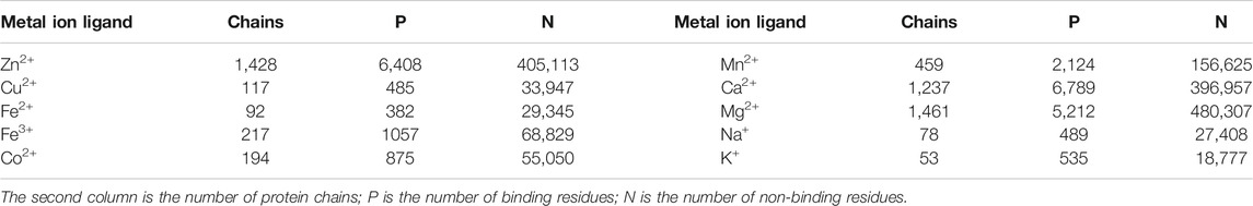
TABLE 1. The benchmark datasets of ten metal ion ligands.

2.2 Selection and Extraction of Feature Parameters

2.2.1 Basic Features Parameters

On the basis of the primary sequence of the protein, we selected the amino acids, and physicochemical and predicted structural information as basic feature parameters. These parameters have been widely used in previous works (Hu et al., 2016a; Cao et al., 2017; Liu et al., 2019; Wang et al., 2019; Liu et al., 2020; Wang et al., 2020). The physicochemical features contain hydrophilic–hydrophobic and polarization charge information. According to the hydrophilic–hydrophobic of amino acids (Pánek et al., 2005), we divided the 20 amino acids into 6 categories. Depending on the charged condition of amino acids after the hydrolysis, we divided the 20 amino acids into 3 categories (Taylor, 1986). The detailed classification is presented in Figure 1.

FIGURE 1

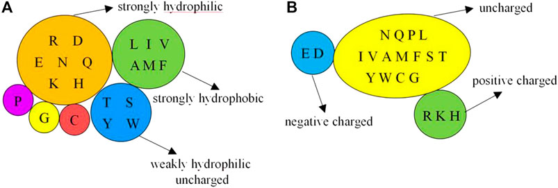
FIGURE 1. Classification of physicochemical features of amino acids. Note: (A) is 6 categories of the hydrophilic–hydrophobic; (B) is 3 categories of the polarization charge.

By using the ANGLOR software (Wu and Zhang, 2008), we obtained the predicted structural features including secondary structure and relative solvent accessibility from the primary sequence of protein. Here, we divided the secondary structure into three categories: α-helix, β-sheet, and coil. In addition, we divided the relative solvent accessibility into two categories: exposed and buried. If the Boolean values of amino acid were larger than 0.25, then the amino acids were defined as “exposed" ones; otherwise, they were defined as “buried” ones.

2.2.2 Amino Acid Correlation Features

We took a detailed statistical analysis for the correlation features of amino acids. According to the analysis results, we calculated the correlation information of amino acids; the detailed steps were as follows:

2.2.2.1 Sequence-Based Correlation Statistical Analysis

Due to protein folding in the 3D structure, one spatial binding site of a metal ion ligand usually refers to several surrounding binding residues. In this way, although the spatial distance of these surrounding residues is very close, the sequence distance may be very long. For example, on the BS01 binding site of the protein (3I11A), the binding residues bound with Co²⁺ ligands were located at 86, 88, 90, and 149 positions in the same sequence, respectively. These binding residues may have long-range correlation (Chen et al., 2018; Zhang et al., 2020). Then, for every protein chain, we scanned from the first binding residue and counted the distance between the two binding residues sequentially. Taking Ca²⁺ and Co²⁺ ligands as examples, the binding residues are shown in Figure 2.

FIGURE 2

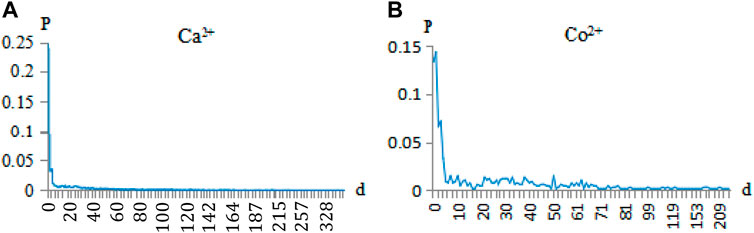
FIGURE 2. Correlation probability of Ca²⁺and Co²⁺ ligand-binding residues. Note: the abscissa d is the correlation of the binding residues (e.g., d = 0 is the adjacent, d = 1 is the secondary neighbor, d = 2 is the thirdly neighbor). The ordinate p is the probability of correlation between the binding residues.

In Figure 2, the correlations of the adjacent, secondary neighbor and thirdly neighbor between binding residues accounted for a large proportion. Since the occurrence probability of d > 6 is not high, we showed the probability of d < 6 for the 10 metal ions in Table 2.

TABLE 2

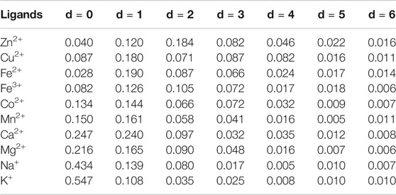
TABLE 2. The correlation probability of 10 metal ion ligand-binding residues.

From Table 2, we found that the probabilities of the adjacent, secondary neighbor, and thirdly neighbor correlations for the ten ions were different. For a metal ion ligand, we selected the correlation information with probability >10% to extract parameters. In this way, for Co²⁺, Mn²⁺, Ca²⁺, Mg²⁺, Na⁺, and K⁺, we extracted the adjacent and secondary neighbor correlation information. For Zn²⁺ and Fe³⁺, we extracted the secondary neighbor and thirdly neighbor correlation information. For Fe²⁺ and Cu²⁺, we extracted the second-neighbor correlation information.

2.2.2.2 Further Screening of Related Features

The probability of the occurrence of 400 pairs of amino acids in the positive and negative sets of each ion ligand was counted separately. We used vector B to represent 20 kinds of amino acids and then made a 20*20 matrix J for the 400 pairs of amino acids. The matrix J of the pairs of amino acid was defined as follows:

$J=B^{T}B={\left(\begin{array}{c}A\\ C\\ D\\ ⋮\\ W\\ Y\end{array}\right)}_{20\times 1}{\left(\begin{array}{cccccc}A& C& D& \cdots & W& Y\end{array}\right)}_{1\times 20}={\left(\begin{array}{cccccc}AA& AC& AD& \cdots & AW& AY\\ CA& CC& CD& \cdots & CW& CY\\ DA& DC& DD& \cdots & DW& DY\\ ⋮& ⋮& ⋮& \ddots & ⋮& ⋮\\ WA& WC& WD& \cdots & WW& WY\\ YA& YC& YD& \cdots & YW& YY\end{array}\right)}_{20\times 20}$

Then, we calculated the D-values of the probability of 400 pairs of amino acids between the negative sets and the positive sets. For example, the D-value differences of correlation information of Cu²⁺ secondary neighbor and Fe³⁺ thirdly neighbor are given in Figures 3, 4, respectively.

FIGURE 3

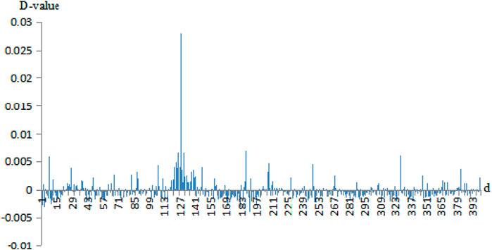
FIGURE 3. The probability difference of the secondary neighbor correlation of Cu²⁺ positive and negative fragments. Note: the abscissa 1–400 is AA, AC, AD, …, AY, CA, CC, CD, …, CY, …, YA, YC, YD, …, YY. The ordinate is the D-values of the positive sets minus the negative sets.

FIGURE 4

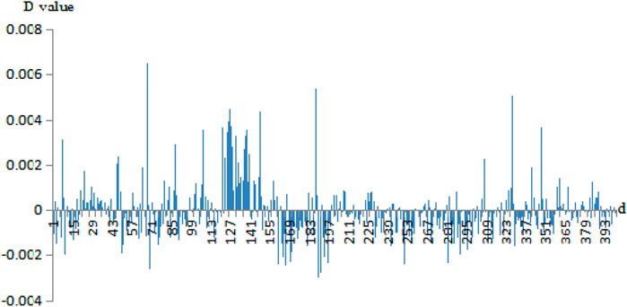
FIGURE 4. The probability difference of the thirdly neighbor correlation of Fe³⁺ positive and negative fragments. Note: the abscissa 1–400 is AA, AC, AD, …, AY, CA, CC, CD, …, CY, …, YA, YC, YD, …, YY. The ordinate is the D-values of the positive sets minus the negative sets.

In Figures 3, 4, the abscissa was the 400 amino acid pairs from matrix J, the corresponding vector (AA, AC, AD, …, AY, CA, CC, CD, …, CY, …, YA, YC, YD, …, YY). The ordinate was the D-values between the positive sets and the negative sets. In Figure 4, If the bars were above the x-axis, it represents that the occurrence probability of amino acids pairs of the positive sets was greater. Otherwise, the probability of the negative sets was greater. In Figure 3, the abscissa values of Cu²⁺ secondary neighbor correlation were 7, 127, 187, and 327; the corresponding AH, HH, LH, and TH pairs of amino acids had a great difference in probability between positive and negative sets. They tended to appear in positive sets; in particular, the HH had a larger difference in probability. In Figure 4, the abscissa values of the Fe³⁺ thirdly neighbor correlation were 67, 126, 147, 187, 327, and 347 corresponding to EH, HG, IH, LH, TH, and VH. They had great probability differences between the positive and negative sets, and preferred to appear in positive sets. Among them, EH, LH, and TH were more obvious. The probability difference of EK, LK, LL, and RA between the positive and negative sets was greater, and these pairs preferred to appear in negative sets.

2.2.2.3 Feature Parameters of Amino Acid Correlation

Due to the fact that the 400 pairs of amino acids appear differently between positive and negative sets, the ones with little difference would cause information redundancy of prediction parameters. Therefore, we sorted the absolute values of the probability difference in descending order obtained from the top 100 features. Then, we divided them into 10 groups in order. Within each group, there were 10 features. Finally, we took the amino acid correlation features as feature parameters.

2.2.3 Binding Residues Propensity Factors

Previous studies on predicting the ligand-binding residues were usually based on the binding residues and their surrounding residues. However, the features of the binding residues alone were not taken into consideration. In fact, the ligand-specific binding also has a selective preference for different amino acid residues. Therefore, we counted the amino acid residues that the 10 metal ion ligands preferred to bind. For example, Zn²⁺ and Fe²⁺ are shown in Figure 5.

FIGURE 5

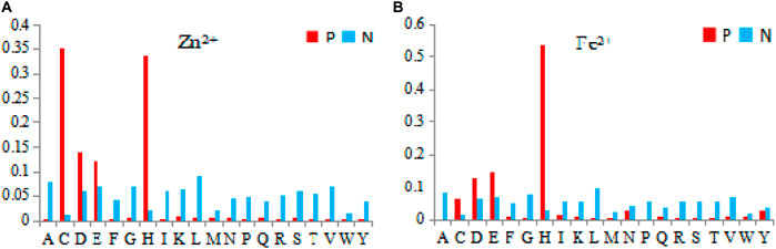
FIGURE 5. The probability of 20 amino acids in Zn²⁺ and Fe²⁺ bounding residues. Note: The abscissa values represents 20 amino acids, the letters of an alphabet in ordinate represents the probability. P represents the binding residue, and N represents the non-binding residue.

In Figure 5, among the 20 amino acids, the four amino acids of C, D, E, and H were more likely to be the binding residues. However, for Zn²⁺ and Fe²⁺ ligands, the four amino acids were used differently. In comparison, C and H were more easily bound by Zn²⁺ ligands, while H was more easily bound by Fe²⁺ ligands. Therefore, we extracted propensity factor of binding residues as feature parameters. The formula of the propensity factor (Chou and Fasman, 1974) was as follows:

$F_{ij}=\frac{p_{ij}}{p_j}(1)$

The statistical samples were binding residues and non-binding residues, $p_{ij}=\frac{n_{ij}}{N_i}$, $p_j=\frac{N_j}{N_t}$; $i$ is 20 amino acids (i = 1,2, … 20); $j$ is binding residues or non-binding residues (j = 1,2); $n_{ij}$ represents the number of amino acid $i$ in binding residues or non-binding residues; $N_i$ represents the number of amino acid $i$ in the statistical samples; $N_j$ represents the number of binding or non-binding residues; $N_t$ represents the number of residues in the statistical samples. If $F_{ij}$ is larger than 1, it means that type amino acid $i$ is more inclined to be amino acid $j$. Taking Mn²⁺ as an example, the values of propensity factor of amino acids D, E, H, and N were larger than 1, indicating that the 4 amino acids were more likely to become binding residues (Table 3).

TABLE 3

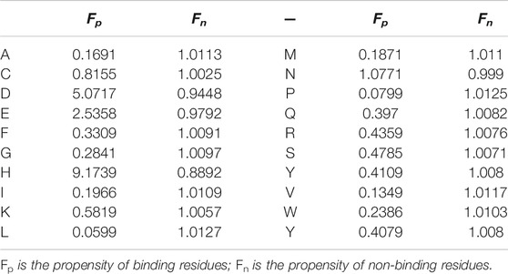
TABLE 3. The binding and non-binding residue amino acid propensity factors of Mn²⁺.

2.2.4 Extraction of Feature Parameters

Besides the propensity factors for feature parameters, we also used components, matrix scoring, and information entropy to extract parameters. First, the component information of amino acids, correlation features, secondary structure, and relative solvent accessibility were extracted. Then, the position weight matrix was used to extract the conservative information of the site as a predictive parameter (Hu et al., 2016a; Liu et al., 2019; Wang et al., 2019; Liu et al., 2020; Wang et al., 2020). In this paper, based on the above matrix, the 2L-dimensional site conservative information of amino acids, secondary structure, and relative solvent accessibility were obtained. The position weight matrix formula was as follows:

$m_{i,j}=\ln \left(\frac{p_{i,j}}{p_{0,j}}\right)(2)$

$p_{i,j}=\frac{n_{i,j}+\frac{\sqrt{N_i}}{q}}{N_i+\sqrt{N_i}}(3)$

Where $i$ denotes the site, $j$ represents 20 amino acids and pseudo-amino acid X, $P_{i,j}$ represents the probability of occurrence of amino acid sites at the ith position, and $P_{0,j}$ represents the background probability. $n_{i,j}$ represents the number of amino acids j at the ith position, $N_i$ represents the number of all amino acids at the ith position, and q represents the number of categories q = 21. Two scoring matrices can be obtained by using positive and negative training sets, and a 2L (L is the window length)-dimensional feature vector can be obtained for arbitrary fragment. Similarly, for the secondary structure (q = 4) and relative solvent accessibility (q = 3), 2L-dimensional site conservation features can also be obtained.

As the number of amino acids included in the classification of the hydrophilic–hydrophobic and polarized charges of amino acids was not uniform, information entropy (Liu et al., 2020; Wang et al., 2020) was used to extract the hydrophilic–hydrophobic and polarized charges. The formulas for information entropy were as follows:

$H\left(x\right)=-\stackrel{q}{\Sigma }{p}_j{\log }_2{p}_j(4)$

$p_j=\frac{\left(n_j+\frac{\sqrt{N}}{q}\right)}{\left(N+\sqrt{N}\right)}(5)$

Where j = 1, 2, … q, q represents the number of categories, $N={\displaystyle \sum _{j=1}^q{n}_j}$, n_j represents the frequency of occurrence of hydrophilic–hydrophobic or polarized charges in the classification, and p_j represents the probability of occurrence of a certain category, hydrophilic–hydrophobic (q = 7) and polarized charge (q = 4). For arbitrary fragment, one-dimensional hydrophilic–hydrophobic information entropy and one-dimensional polarization charge information entropy can be obtained.

2.3 Gradient Boosting Machine Algorithm

As an improved Boosting algorithm, GBM algorithm was proposed by Friedman (2001). It achieved excellent results in many data mining competitions and was widely used in many fields (Feng and Li, 2017; Rawi et al., 2017; Hu et al., 2020). The advantage of the GBM is that it inherits the advantages of a single decision tree and discards its shortcomings. It can fit complex nonlinear relationships with fast calculation speed, strong robustness, and high accuracy. The deviation of the model will not have a serious impact on the algorithm. The GBM improves the model by adding a new classifier to continuously decrease the overall residual; after the iteration, the classifier is as follows:

$F_m\left(x\right)=F_{m-1}\left(x\right)+{\rho }_m{h}_m\left(x\right)(6)$

Where m is the number of iterations, ${\rho }_m$ is the weight value (the distance the loss function drops in its gradient direction), and $h_m\left(x\right)$ is the fitting function of the sample residuals $y-F_{m-1}\left(x\right)$ in the iteration process.

This article used the “gbm” package in R software version 3.6.3. Here, in the algorithm, we mainly optimized the four adjustable parameters (i.e., n.trees, interaction.depth, shrinkage, and n.minobsinnode) (Rawi et al., 2017; Hu et al., 2020).

2.4 The Validation Methods and Evaluation Metrics

The 5-fold cross-validation was generally used to identify binding residues (Hu et al., 2016a; Hu et al., 2016b; Liu et al., 2019; Wang et al., 2019; Liu et al., 2020; Wang et al., 2020). The following 4 evaluation indicators were used to evaluate the recognition ability of the prediction model (Jiao and Du, 2016; Chen et al., 2019): sensitivity (S_n), specificity (S_p), accuracy (Acc), and Matthew’s correlation coefficient (MCC). The formulas were defined as follows:

$S_n=\frac{TP}{TP+FN}\times 100\%(7)$

$S_p=\frac{TN}{TN+FP}\times 100\%(8)$

$Acc=\frac{TP+TN}{TP+TN+FP+FN}\times 100\%(9)$

$MCC=\frac{\left(TP\times TN\right)-\left(FP\times FN\right)}{\sqrt{\left(TP+FP\right)\left(TP+FN\right)\left(TN+FP\right)\left(TN+FN\right)}}(10)$

In the above formulas, TP is the number of correctly predicted binding residues, FN is the number of incorrectly predicted binding residues, TN is the number of correctly predicted non-binding residues, and FP is the number of incorrectly predicted non-binding residues.

3 Calculation Results and Discussion

3.1 The Prediction Framework

The prediction parameters from Sections 2.2.3, 2.2.4 are summarized and shown in Table 4. The work flow of identifying the ion ligand binding sites is shown in Figure 6.

TABLE 4

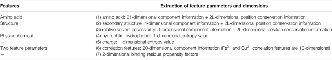
TABLE 4. A summary of prediction parameters.

FIGURE 6

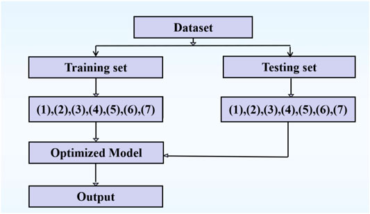
FIGURE 6. The work flow of identifying the ion ligand binding sites. Note: (1), (2), (3), …, (7) represent the different types of features.

3.2 Results and Discussion

In prediction, we used the full parameters of Table 5 and input the combined features into the GBM algorithm. Then, we calculated the results of 7 window lengths (i.e., 5, 7, 9, 11, 13, 15, and 17) on a 5-fold cross-validation test. In the process, we defined the corresponding window lengths as the optimal ones (L) with higher S_n and MCC values. The predicted results of GBM⁽¹⁾ with the optimal window are shown in Table 5.

TABLE 5

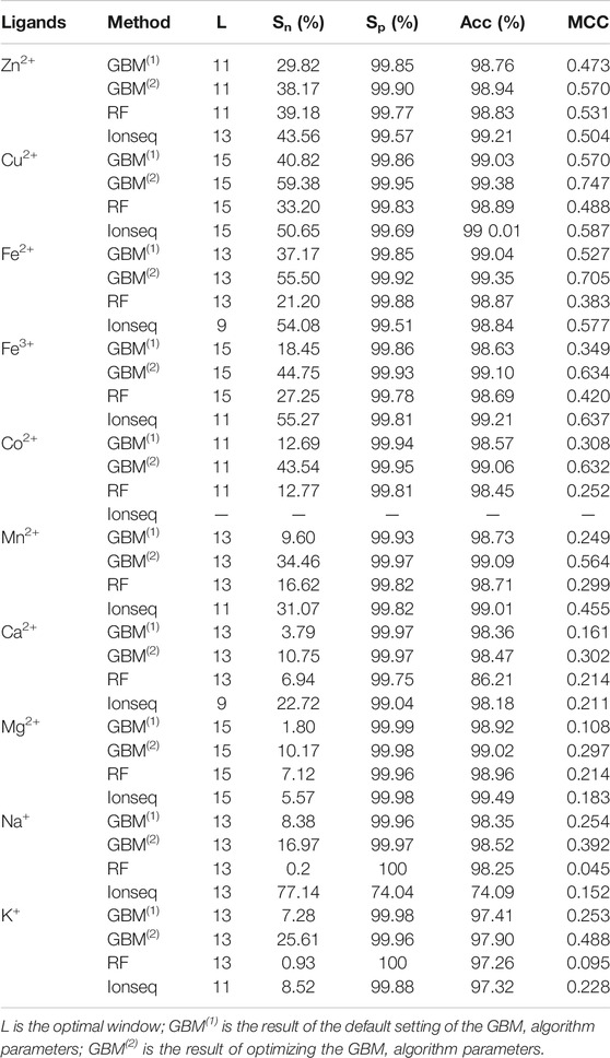
TABLE 5. Comparison of 5-fold cross-validation results.

In the results of GBM⁽¹⁾ (Table 5), the predicted results of transition-metal ion ligands were better. The S_n and MCC values of Zn²⁺, Cu²⁺, and Fe²⁺ ligands were higher than 29.82% and 0.473, respectively. The S_n and MCC values of Fe³⁺, Co²⁺, and Mn²⁺ ligands were higher than 9.6% and 0.249, respectively. The S_n and MCC values of alkali–metal ion ligands were higher than 7.28% and 0.253, respectively.

In order to test the validity of the amino acid correlation information and binding residue propensity factor, we removed correlation features or propensity factors from the full feature sets. Taking Cu²⁺ and Na⁺ ligands as examples, the results are shown in Table 6.

TABLE 6

TABLE 6. The results of 5-fold cross-validation.

In comparison with (a), for Cu²⁺ ligand: the S_n and MCC values of (b) were higher, and S_n and MCC values of (c) increased by 10.1% and 0.072, respectively. When parameters of correlation feature and propensity factor were added, the S_n and MCC value were significantly increased by 11.54% and 0.109, respectively. For Na⁺ ligand: the Sn and MCC values of (b) were significantly improved by 5.32% and 0.112, respectively. The Sn and MCC values of (c) were increased. When correlation feature and propensity factor were added, the S_n and MCC values increased by 6.54% and 0.138, respectively.

On the addition of feature parameters, different metal ion ligands have different sensitivities. For instance, the Cu²⁺ ligand was more sensitive to the propensity factor, while the Na⁺ ligand was more sensitive to the correlation feature. Above all, the results of adding two parameters were better than those of adding one alone.

In order to further improve the prediction accuracy, we optimized the four parameters (e.g., n.trees, interaction.depth, shrinkage, and n.minobsinnode) in the GBM algorithm. According to the reported literature (Rawi et al., 2017; Hu et al., 2020), the parameter range was set as follows: n.trees in n{100,150,200,250,300,350,400,450,500}, interaction.depth in d{3,5,7,9}, shrinkage in r{0.01,0.1}, and n.minobsinnode in m{10,20,30,40,50}. The AUROC values were used as the evaluation indicator to obtain the optimal algorithm parameters by the grid search method. Taking Cu²⁺ and K⁺ ligands as examples, the optimal parameters of Cu²⁺ ligand were (5,250,0.1,40), and the AUROC value was 0.985. The optimal parameters of K⁺ ligand were (9,200,0.1,10), and the AUROC value was 0.963. The ROC curves corresponding to the optimal parameters of Cu²⁺ and K⁺ ligands are shown in Figure 7.

FIGURE 7

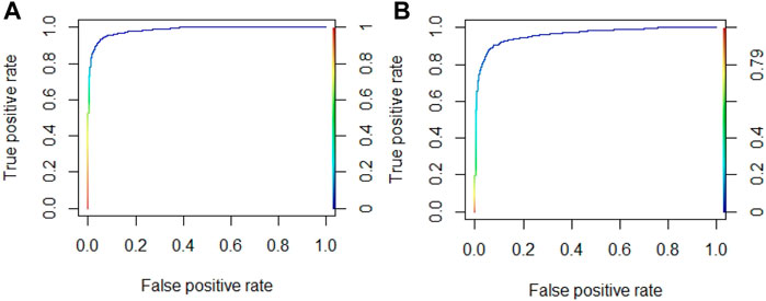
FIGURE 7. The ROC curve of optimal algorithm parameters for Cu²⁺and K⁺ ligands. Note: (A) is Cu²⁺ ligand; (B) is K⁺ ligand.

As can be seen in Figure 6, the AUROC values of Cu²⁺ and K⁺ ligands both exceed 0.96. For the convenience of comparison, the results after optimizing the algorithm parameters were also added in Table 6.

From the results of GBM⁽²⁾ in Table 6, it can be seen that the values of S_n and MCC of transition metal ion ligands were higher than 34.46% and 0.564, respectively. The values of S_n and MCC in the results of alkaline Earth metal ion ligands were higher than 10.17% and 0.297, respectively. The values of S_n and MCC in the results of alkali metal ion ligands were higher than 16.97% and 0.392, respectively. In comparison with the results of GBM⁽¹⁾, the results of GBM⁽²⁾ were significantly improved, in which the S_n and MCC values of the nine ligands (i.e., Cu²⁺, Fe²⁺, Fe³⁺, Co²⁺, Mn²⁺, Ca²⁺, Mg²⁺, Na⁺, and K⁺) increased by more than 6.96% and 0.141, respectively.

To verify the stability of those parameters in prediction, the Random Forest (RF) algorithm was also used on the same parameters. The number of decision trees in the RF was set as 500 (Liaw and Wiener, 2002; Liu et al., 2020). The results of the RF were added in Table 6. Except for the alkali metal ion ligands, the S_n and MCC values of the other ion ligands were higher than 6.94% and 0.214. The predicted results of transition metal ion ligands were better. The S_n and MCC values of Zn²⁺, Cu²⁺, and Fe³⁺ ligands were higher than 27.25% and 0.420, respectively. The S_n and MCC values of Fe²⁺, Co²⁺, and Mn²⁺ ligands were higher than 12.27% and 0.252, respectively. Taken together, with the same parameters by using RF, we also obtained good predicted results. Except for Zn²⁺, the results of GBM⁽²⁾ were better than those of RF algorithm. For Cu²⁺, Fe²⁺, Co²⁺, Na⁺, and K⁺ ligands, the S_n and MCC values were at least 26.18% and 0.259 higher in the GBM algorithm. For Fe³⁺ and Mn²⁺ ligands, the S_n and MCC values were at least 17.5% and 0.214 higher, respectively.

In the field of predicting metal ion ligand-binding residues, Hu et al. (2016a) proposed several predicted methods and obtained well-predicted results. At present, the Ionseq is a method with better predicted results on the unbalanced datasets. Thus, we took a comparison with the method of Ionseq in Table 6. It can be seen that the S_n and MCC values of Cu²⁺, Fe²⁺, Mn²⁺, Mg²⁺, and K⁺ ligands were better than those of Ionseq. Due to the fact that the number of binding residues was far less than the number of non-binding residues, it would lead to a high false positive. In order to show the improvement, we took a random protein chain (2 × 11A) bound by Cu²⁺ ligand as an example. Based on the above optimal model, we made a prediction for this protein chain. The predicted results obtained are shown in Figure 8.

FIGURE 8

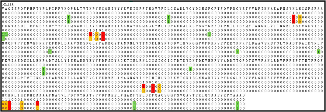
FIGURE 8. The comparison of identification results. Note: The first row is the protein sequence, the second row is the experimental results, the third row is the optimal predicted results, and the fourth row is the predicted results using the basic parameters. “0” is the non-binding residue, “1” is the binding residue. The red ones indicate TP. The white ones indicate TN. The yellow ones indicate FN. The green ones indicate FP.

By comparing the second and third rows, we obtained that the prediction results of the optimal model (GBM⁽²⁾) were TP = 7, TN = 509, FP = 6, and FN = 11. By comparing the second and fourth rows, the prediction results of the prediction model with basic feature parameters were TP = 4, TN = 514, FP = 6, and FN = 9. The comparison showed that the prediction results were significantly improved after adding correlation features and propensity factors.

5 Conclusion

In this paper, based on the primary sequence information, the amino acid correlation features and binding residue propensity factors were added as feature parameters for the prediction of the metal ion ligand-binding residues. In comparison with previous works, our improved results proved that the features of amino acid correlation information and propensity factor information were beneficial to the identification of the metal ion ligand-binding residues. With the optimized parameters, the results of GBM were better than those of RF on the same parameters. Therefore, we believe that our proposed method was a valuable tool to identify metal ion ligand-binding residues.

Data Availability Statement

The datasets presented in this study can be found in online repositories. The names of the repository/repositories and accession number(s) can be found below: BioLip. (http://zhanglab.ccmb.med.umich.edu/BioLiP/) The key data sets of our work were available in the Supplementary File.

Author Contributions

SX: Mainly responsible for data calculation and article writing; XH: Provided research guidance and wrote the article; ZF: Assisted in writing the article and foreign language translation; JP: Provided guidance in the writing of the article; KS: Assisted in the writing of the first draft; XY: Assisted in calculating data and analysis; ZW: Assisted in organizing datasets.

Funding

This work was supported by the National Natural Science Foundation of China (61961032 and 31260203), the Natural Science Foundation of the Inner Mongolia of China (2019BS03025), and the Natural Science Foundation of Inner Mongolia University of Technology (ZY201915).

Conflict of Interest

The authors declare that the research was conducted in the absence of any commercial or financial relationships that could be construed as a potential conflict of interest.

Publisher’s Note

All claims expressed in this article are solely those of the authors and do not necessarily represent those of their affiliated organizations, or those of the publisher, the editors, and the reviewers. Any product that may be evaluated in this article, or claim that may be made by its manufacturer, is not guaranteed or endorsed by the publisher.

Supplementary Material

The Supplementary Material for this article can be found online at: https://www.frontiersin.org/articles/10.3389/fgene.2021.793800/full#supplementary-material

References

Barnham, K. J., and Bush, A. I. (2008). Metals in Alzheimer's and Parkinson's Diseases. Curr. Opin. Chem. Biol. 12 (2), 222–228. doi:10.1016/j.cbpa.2008.02.019

PubMed Abstract | CrossRef Full Text | Google Scholar

Barondeau, D. P., and Getzoff, E. D. (2004). Structural Insights into Protein-Metal Ion Partnerships. Curr. Opin. Struct. Biol. 14 (6), 765–774. doi:10.1016/j.sbi.2004.10.012

PubMed Abstract | CrossRef Full Text | Google Scholar

Cao, X., Hu, X., Zhang, X., Gao, S., Ding, C., Feng, Y., et al. (2017). Identification of Metal Ion Binding Sites Based on Amino Acid Sequences. Plos One 12 (8), e0183756. doi:10.1371/journal.pone.0183756

PubMed Abstract | CrossRef Full Text | Google Scholar

Cecconi, I., Scaloni, A., Rastelli, G., Moroni, M., Vilardo, P. G., Costantino, L., et al. (2002). Oxidative Modification of Aldose Reductase Induced by Copper Ion. J. Biol. Chem. 277 (44), 42017–42027. doi:10.1074/jbc.m206945200

CrossRef Full Text | Google Scholar

Chen, Z., Zhao, P., Li, F., Leier, A., Marquez-Lago, T. T., Wang, Y., et al. (2018). iFeature: a Python Package and Web Server for Features Extraction and Selection from Protein and Peptide Sequences. Bioinformatics 34 (14), 2499–2502. doi:10.1093/bioinformatics/bty140

PubMed Abstract | CrossRef Full Text | Google Scholar

Chen, Z., Zhao, P., Song, J. N., Marquez-Lago, T. T., Leier, A., Revote, J., et al. (2019). iLearn: an Integrated Platform and Meta-Learner for Feature Engineering, Machine Learning Analysis and Modeling of DNA, RNA and Protein Sequence Data[J]. Brief. Bioinform. 21, 1047. doi:10.1093/bib/bbz041

CrossRef Full Text | Google Scholar

Chou, P. Y., and Fasman, G. D. (1974). Conformational Parameters for Amino Acids in Helical, β-sheet, and Random Coil Regions Calculated from Proteins. Biochemistry 13 (2), 211–222. doi:10.1021/bi00699a001

PubMed Abstract | CrossRef Full Text | Google Scholar

Feng, Z. X., and Li, Q. Z. (2017). Recognition of Long-Range Enhancer-Promoter Interactions by Adding Genomic Signatures of Segmented Regulatory Regions. Genomics 109 (5-6), 341–352. doi:10.1016/j.ygeno.2017.05.009

PubMed Abstract | CrossRef Full Text | Google Scholar

Friedman, J. H. (2001). Greedy Function Approximation:A Gradient Boosting Machine[J]. Tne Ann. Stat. 29 (5), 1189–1232. doi:10.1214/aos/1013203451

CrossRef Full Text | Google Scholar

Horst, J. A., and Samudrala, R. (2010). A Protein Sequence Meta-Functional Signature for Calcium Binding Residue Prediction. Pattern recognition Lett. 31 (14), 2103–2112. doi:10.1016/j.patrec.2010.04.012

CrossRef Full Text | Google Scholar

Hu, X., Dong, Q., Yang, J., and Zhang, Y. (2016). Recognizing Metal and Acid Radical Ion-Binding Sites by Integratingab Initiomodeling with Template-Based Transferals. Bioinformatics 32 (21), 3260–3269. doi:10.1093/bioinformatics/btw396

PubMed Abstract | CrossRef Full Text | Google Scholar

Hu, X., Feng, Z., Zhang, X., Liu, L., and Wang, S. (2020). The Identification of Metal Ion Ligand-Binding Residues by Adding the Reclassified Relative Solvent Accessibility. Front. Genet. 11, 214. doi:10.3389/fgene.2020.00214

PubMed Abstract | CrossRef Full Text | Google Scholar

Hu, X., Wang, K., and Dong, Q. (2016). Protein Ligand-specific Binding Residue Predictions by an Ensemble Classifier. BMC Bioinformatics 17 (1), 470–481. doi:10.1186/s12859-016-1348-3

PubMed Abstract | CrossRef Full Text | Google Scholar

Jiang, Z., Hu, X. Z., Geriletu, G., Xing, H. R., and Cao, X. Y. (2016). Identification of Ca(2+)-Binding Residues of a Protein from its Primary Sequence. Genet. Mol. Res. 15 (2), 15027618. doi:10.4238/gmr.15027618

CrossRef Full Text | Google Scholar

Jiao, Y., and Du, P. (2016). Performance Measures in Evaluating Machine Learning Based Bioinformatics Predictors for Classifications. Quant Biol. 4 (4), 320–330. doi:10.1007/s40484-016-0081-2

CrossRef Full Text | Google Scholar

Liaw, A., and Wiener, M. (2002). Classification and Regression by Random Forest[J]. R. News 2 (3), 18–22.

Google Scholar

Liu, L., Hu, X., Feng, Z., Wang, S., Sun, K., and Xu, S. (2020). Recognizing Ion Ligand-Binding Residues by Random Forest Algorithm Based on Optimized Dihedral Angle. Front. Bioeng. Biotechnol. 8, 493. doi:10.3389/fbioe.2020.00493

PubMed Abstract | CrossRef Full Text | Google Scholar

Liu, L., Hu, X., Feng, Z., Zhang, X., Wang, S., Xu, S., et al. (2019). Prediction of Acid Radical Ion Binding Residues by K-Nearest Neighbors Classifier. BMC Mol. Cel Biol 20 (Suppl. 3), 52. doi:10.1186/s12860-019-0238-8

PubMed Abstract | CrossRef Full Text | Google Scholar

Lu, C.-H., Lin, Y.-F., Lin, J.-J., and Yu, C.-S. (2012). Prediction of Metal Ion-Binding Sites in Proteins Using the Fragment Transformation Method. Plos One 7 (6), e39252. doi:10.1371/journal.pone.0039252

PubMed Abstract | CrossRef Full Text | Google Scholar

Pánek, J., Eidhammer, I., and Aasland, R. (2005). A New Method for Identification of Protein (Sub)families in a Set of Proteins Based on Hydropathy Distribution in Proteins[J]. Proteins 58 (4), 923–934.

PubMed Abstract | Google Scholar

Petris, M. J., Mercer, J. F., Culvenor, J. G., Lockhart, P., Gleeson, P. A., and Camakaris, J. (1996). Ligand-regulated Transport of the Menkes Copper P-type ATPase Efflux Pump from the Golgi Apparatus to the Plasma Membrane: a Novel Mechanism of Regulated Trafficking. EMBO J. 15 (22), 6084–6095. doi:10.1002/j.1460-2075.1996.tb00997.x

PubMed Abstract | CrossRef Full Text | Google Scholar

Rawi, R., Mall, R., Kunji, K., Shen, C.-H., Kwong, P. D., and Chuang, G.-Y. (2017). PaRSnIP: Sequence-Based Protein Solubility Prediction Using Gradient Boosting Machine. Bioinformatics 34 (7), 1092–1098. doi:10.1093/bioinformatics/btx662

CrossRef Full Text | Google Scholar

Reed, G. H., and Poyner, R. R. (2000). Mn2+ as a Probe of Divalent Metal Ion Binding and Function in Enzymes and Other Proteins. Met. Ions Biol. Syst. 37 (12), 183–207.

PubMed Abstract | Google Scholar

Taylor, W. R. (1986). The Classification of Amino Acid Conservation. J. Theor. Biol. 119 (2), 205–218. doi:10.1016/s0022-5193(86)80075-3

CrossRef Full Text | Google Scholar

Wang, S., Hu, X., Feng, Z., Zhang, X., Liu, L., Sun, K., et al. (2019). Recognizing Ion Ligand Binding Sites by SMO Algorithm. BMC Mol. Cel Biol 20 (Suppl. 3), 53. doi:10.1186/s12860-019-0237-9

PubMed Abstract | CrossRef Full Text | Google Scholar

Wang, S., Hu, X. Z., Feng, Z. X., Liu, L., Sun, K., and Xu, S. (2020). Recognition of Ion Ligand Binding Sites Based on Amino Acid Features with the Fusion of Energy, Physicochemical and Structural Features[J]. Curr. Pharm. Des. 26, 1093. doi:10.2174/1381612826666201029100636

PubMed Abstract | CrossRef Full Text | Google Scholar

Wu, S., and Zhang, Y. (2008). ANGLOR: A Composite Machine-Learning Algorithm for Protein Backbone Torsion Angle Prediction. Plos One 3 (10), e3400. doi:10.1371/journal.pone.0003400

PubMed Abstract | CrossRef Full Text | Google Scholar

Yang, J., Roy, A., and Zhang, Y. (2013). BioLiP: a Semi-manually Curated Database for Biologically Relevant Ligand-Protein Interactions. Nucleic Acids Res. 41 (D1), D1096–D1103. doi:10.1093/nar/gks966

PubMed Abstract | CrossRef Full Text | Google Scholar

Yang, J., Roy, A., and Zhang, Y. (2013). Protein-ligand Binding Site Recognition Using Complementary Binding-specific Substructure Comparison and Sequence Profile Alignment. Bioinformatics 29 (20), 2588–2595. doi:10.1093/bioinformatics/btt447

PubMed Abstract | CrossRef Full Text | Google Scholar

Yuan, D. S., Stearman, R., Dancis, A., Dunn, T., Beeler, T., and Klausner, R. D. (1995). The Menkes/Wilson Disease Gene Homologue in Yeast Provides Copper to a Ceruloplasmin-like Oxidase Required for Iron Uptake. Proc. Natl. Acad. Sci. 92 (7), 2632–2636. doi:10.1073/pnas.92.7.2632

PubMed Abstract | CrossRef Full Text | Google Scholar

Zhang, W. Y., Xu, J., Wang, J., Zhou, Y-K., Chen, W., and Du, P-F. (2020). KNIndex: a Comprehensive Database of Physicochemical Properties for K-Tuple Nucleotides[J]. Brief. Bioinform. 22, bbaa284. doi:10.1093/bib/bbaa284

PubMed Abstract | CrossRef Full Text | Google Scholar