
95% of researchers rate our articles as excellent or good
Learn more about the work of our research integrity team to safeguard the quality of each article we publish.
Find out more
ORIGINAL RESEARCH article
Front. Genet. , 23 November 2021
Sec. Livestock Genomics
Volume 12 - 2021 | https://doi.org/10.3389/fgene.2021.717409
This article is part of the Research Topic Genotype-by-Environment Interaction in Farm Animals: From Measuring to Understanding View all 5 articles
 P. H. F. Freitas1
 J. S. Johnson2
 S. Chen1,3
 H. R. Oliveira1,4
 F. Tiezzi5S. F. Lázaro1,6
 Y. Huang7Y. Gu7
 A. P. Schinckel1
 L. F. Brito1*
Properly quantifying environmental heat stress (HS) is still a major challenge in livestock breeding programs, especially as adverse climatic events become more common. The definition of critical periods and climatic variables to be used as the environmental gradient is a key step for genetically evaluating heat tolerance (HTol). Therefore, the main objectives of this study were to define the best critical periods and environmental variables (ENV) to evaluate HT and estimate variance components for HT in Large White pigs. The traits included in this study were ultrasound backfat thickness (BFT), ultrasound muscle depth (MDP), piglet weaning weight (WW), off-test weight (OTW), interval between farrowing (IBF), total number of piglets born (TNB), number of piglets born alive (NBA), number of piglets born dead (NBD), number of piglets weaned (WN), and weaning to estrus interval (IWE). Seven climatic variables based on public weather station data were compared based on three criteria, including the following: (1) strongest G×E estimate as measured by the slope term, (2) ENV yielding the highest theoretical accuracy of the genomic estimated breeding values (GEBV), and (3) variable yielding the highest distribution of GEBV per ENV. Relative humidity (for BFT, MDP, NBD, WN, and WW) and maximum temperature (for OTW, TNB, NBA, IBF, and IWE) are the recommended ENV based on the analyzed criteria. The acute HS (average of 30 days before the measurement date) is the critical period recommended for OTW, BFT, and MDP in the studied population. For WN, WW, IBF, and IWE, a period ranging from 34 days prior to farrowing up to weaning is recommended. For TNB, NBA, and NBD, the critical period from 20 days prior to breeding up to 30 days into gestation is recommended. The genetic correlation values indicate that the traits were largely (WN, WW, IBF, and IWE), moderately (OTW, TNB, and NBA), or weakly (MDP, BFT, and NBD) affected by G×E interactions. This study provides relevant recommendations of critical periods and climatic gradients for several traits in order to evaluate HS in Large White pigs. These observations demonstrate that HT in Large White pigs is heritable, and genetic progress can be achieved through genetic and genomic selection.
The incidence and severity of adverse climatic conditions is increasing as a result of climate change, and this has the potential to negatively impact livestock production (Vilas Boas Ribeiro et al., 2018; Bernabucci, 2019). Specifically, climate change-induced heat stress (HS) is considered a major welfare and production issue in the swine industry, especially as advances in genetic selection, nutrition, and management have increased pig performance (Kemp et al., 2018) and subsequently metabolic heat production (Stinn and Xin, 2014; Cabezón et al., 2016). Therefore, improving measures of swine performance and welfare under HS conditions is a primary objective of the global swine industry.
Improved climatic resilience can be achieved by crossbreeding thermally sensitive animals with more heat-tolerant (HT) breeds. Despite the favorable adaptation to HS, a result of these crosses is relatively low production (in comparison to the more productive breeds), which is not profitable under intensive production systems (Berman, 2011; Misztal, 2017). The losses in the swine industry associated with HS are mainly explained by reduced and inconsistent growth, decreased carcass quality, lower feed efficiency, poor sow performance, and increased mortality and morbidity (Renaudeau et al., 2012; Baumgard and Rhoads, 2013; Mayorga et al., 2018). Due to these negative effects and inherent differences in climate, nutrition, and management between nucleus and commercial swine farms, the consideration of genotype-by-environment (G×E) interaction is important for the identification of HT animals. Thereafter, HT animals can be used in reproduction schemes to improve the phenotypic performance of economically important traits (i.e., reproductive, growth, and body composition traits).
The genetic variability for HTol in livestock species has been previously reported (e.g., Carabaño et al., 2017; Misztal, 2017; Ansari-Mahyari et al., 2019; Zhang et al., 2019; Tiezzi et al., 2020). In general, the genetic analyses of HS in pigs are based on heat-load function for live or carcass weight in growing/finishing pigs and are usually emphasized in the sire lines (Zumbach et al., 2008; Fragomeni et al., 2016). Random regression models, more specifically linear reaction norm models (RNM), are commonly used to study G×E interactions (Rauw and Gomez-Raya, 2015), as they allow to better account for variations in HS (Fragomeni et al., 2016). With the use of RNM, the phenotypic values of each animal are randomly regressed on the environmental gradient. This approach generates a regression intercept and slope for each animal, allowing the study of across-environment genetic merit of individuals as well as their potential responsiveness to the environmental changes (Rauw and Gomez-Raya, 2015). Therefore, breeding values and genetic parameters can change gradually along the environmental gradient, and traits may have different means and (co)variances at different environments (Song et al., 2020). These models are applicable when there is a continuous environmental variable that can be used to explore the G×E interaction [e.g., contemporary group effect (CGe), temperature, relative humidity (RH), and temperature–humidity index (THI)].
A genetic or genomic evaluation that accounts for HS requires each record to be associated with some easy-to-measure environmental variables (ENV). Several studies have focused on alternative environmental gradients, such as estimated average performance of CGe (Li and Hermesch, 2016; Song et al., 2020; Chen et al., 2021) and climatic variables (Fragomeni et al., 2016; Tiezzi et al., 2020; Usala et al., 2021). However, the best environmental metrics and critical periods to be used when evaluating HTol in maternal-line pigs need to be comprehensively evaluated to generate accurate estimations of breeding values. In this regard, the main objectives of this study were to (1) define the best environmental descriptors based on public weather station information and critical periods to evaluate HTol and (2) estimate variance components for HTol for populations of Large White pigs (one of the main maternal-line breeds in the world).
Animal welfare and ethics committee approval was not needed for this study, as all the datasets used were provided by commercial breeding operations.
All datasets were provided by the Smithfield Premium Genetics company (Rose Hill, North Carolina, US). Phenotypic nucleus-herd records were obtained from January 2004 to December 2019 for Large White animals distributed among 33 farms located across North America. The farm latitudes range from 34° to 42° north, and the longitudes range from -77° to -113°. Different management strategies have been used across farms, such as equipment to alleviate heat stress. However, these practices changed over time, and this information was not recorded. Moreover, the systematic effects included in the statistical models (e.g., contemporary group–CG) are assumed to account for these effects. The traits analyzed were related to body composition [ultrasound backfat thickness (BFT; mm) and ultrasound muscle depth (MDP; mm)], growth [weaning weight of the piglets (WW; kg) and off-test weight (OTW; kg; approximately measured at around 5.5 months of age)], and reproduction [interval between farrow (IBF; days), total number of piglets born (TNB), number of piglets born alive (NBA), number of piglets born dead (NBD), number of piglets weaned (WN), and weaning to estrus interval (IWE; days)]. Contemporary groups (CG) were defined by the concatenation of farrowing year, farrowing season, and farrowing farm for the reproductive traits and of birth year, birth season, and birth farm for the growth and body composition traits, respectively. The phenotypic datasets were edited independently for each trait by removing records deviating ±3.5 SD from the mean. In addition, CG with less than 10 records were removed from further analyses. The descriptive statistics and the number of animals for each studied trait are presented in Table 2.
A total of 265,943 animals were included in the pedigree, which represented more than 10 generations. A total of 8,992 animals were genotyped using the PorcineSNP10K (8,652 SNPs for 886 animals), PorcineSNP50K (50,549 SNPs for 5,706 animals), PorcineSNP60K (57,019 SNPs for 865 animals), and PorcineSNP80K (64,577 SNPs for 1,535 animals) Bead Chips (Illumina, San Diego, CA, United States). In each SNP panel, animals with genotype call rate smaller than 0.90 were removed. Genotype imputation was performed using the FImpute v3 software (Sargolzaei et al., 2014). The missing genotypes were imputed first from the 10K to the 50K panel and then from the 50K or 60K to the 80K panel. The detailed imputation process was described in Chen et al. (2021). Quality control (QC) of genotype data consisted of removing SNPs with call rate below 0.90, minor allele frequency lower than 0.01, and difference between observed and expected heterozygous frequencies lower than 0.15. The genomic QC was implemented in the BLUPF90 family software (Misztal et al., 2018). In the end, 55,375 SNPs for 8,686 animals (7,017 female and 1,669 male) were included in the subsequent analyses.
Public weather station records for all farms were obtained from the Local Climatological Data at the National Oceanic and Atmosphere Administration (www.ncdc.noaa.gov/cdo-web/datatools/lcd?prior%2520=%2520N). Based on the location of the farms, climatic information was collected from the nearest airports. The average distance between an airport and the farm was 30 km (ranging from 7 to 64 km). Seven ENV were evaluated, including the average of mean temperature (MeanT), average of maximum temperature (MaxT), average of minimum temperature (MinT), dew point (DewP), average relative humidity (RH), average discomfort index (DI; Thom, 1959), and average THI calculated as in the Guide to Environmental Research on Animals (NRC, 1971). The average of the raw ENV was used as the environmental covariate. Supplementary Table S1 shows the description of the ENV range for TNB.
The critical periods evaluated in this study were chosen based on physiological knowledge (Johnson et al., 2015; Gonzalez-Rivas et al., 2020; Johnson et al., 2020) of heat stress and were trait dependent. The specific critical periods are shown in Table 1. Both chronic (i.e., HS during the entire grow-finish period; average of 120 days prior to measurement date) and acute (i.e., HS in the last 30 days prior to harvest) HS might have great impact in carcass-related traits, such as OTW, MDP, and BFT and, therefore, were evaluated for the mentioned traits. In addition, pigs exposed to in utero HS have been reported to develop a variety of postnatal phenotypes that prevent profitable production and compromised health and welfare in commercial production systems (Johnson et al., 2020; Maskal et al., 2020). These responses to HS are related to alteration of postnatal response, that is, change of core body temperature. With more intense HS, lactating sows have increased intestinal epithelial hyperpermeability and reduced reproduction (Mayorga et al., 2020). In utero heat stress can also impact long-term growth performance and decrease postnatal growth rates (Johnson et al., 2020; Maskal et al., 2020). Heat-stressed lactating sows also reduce feed intake as a mechanism to minimize metabolic heat production (Renaudeau et al., 2012; Williams et al., 2013; Cabezón et al., 2016). As such, in this study, two different critical periods were evaluated for IBF, IWE, WW, and WN: the first, a period ranging from the last stage of gestation (around day 80) until the farrowing date, and the second, a critical period ranging from the last stage of gestation throughout lactation until the weaning date. Regarding TNB, NBA, and NBD, only one critical period was evaluated. Early studies showed that the first weeks of gestation have a greater impact in the number of viable embryos (Edwards et al., 1968; Omtvedt et al., 1971; Wildt et al., 1975). Therefore, for TNB, NBA, and NBD, the average ENV ranging from 20 days before breeding to 30 days into gestation was considered.
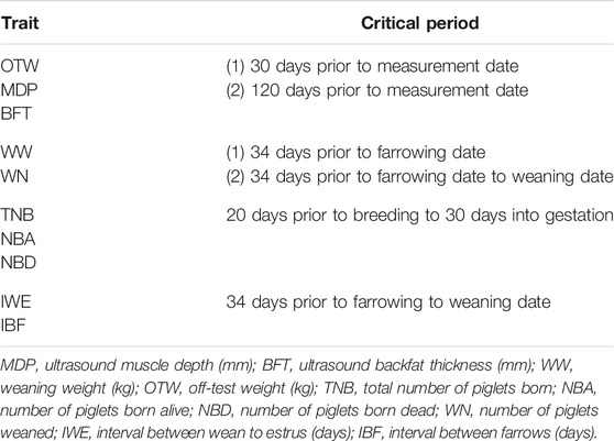
TABLE 1. Description of the critical periods evaluated for each trait to be used for the genetic and genomic evaluation of heat stress in pigs.
Chen et al. (2021), using data from the same population, performed an evaluation of G×E interaction based on CGe. In brief, they estimated variance components and individual breeding values for seven traits (OTW, MDP, BFT, TNB, NBA, WN, and WW), regressing their phenotype on the average effect of CG (Chen et al., 2021). The results obtained in the current study will be compared to the previous results based on the following comparison criteria: theoretical accuracy of genomic estimated breeding values (GEBV) and rank correlation between the GEBV of individuals regressed on the recommended ENV and CGe.
The best statistical model to describe each trait was defined in two steps: (1) the systematic (fixed) effects were defined based on the backwards elimination procedure using the lm function available in the software R (R Core Team, 2020) and (2) the random effects for each trait were defined using the BLUPF90 software (Masuda, 2018; Misztal et al., 2018) by comparing models, including a different combination of random effects [i.e., animal genetic effect, animal permanent environmental effect, and common environment (litter) effect]. Model comparisons were made, and the significant random effects were defined based on the Akaike Information Criterion (Akaike, 1973). Specific and detailed information regarding the definition of the models can be found in Chen et al. (2021). The final effects for each trait are shown in Table 2.
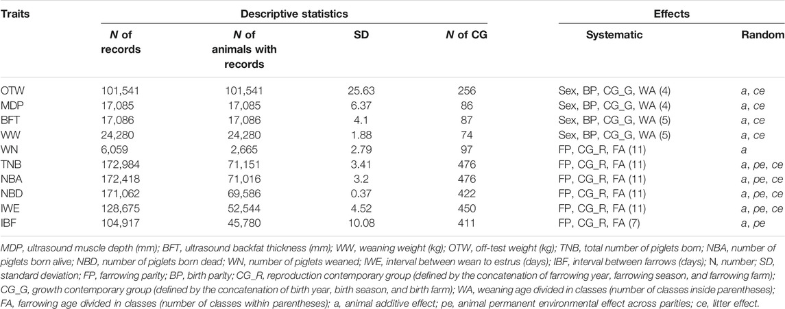
TABLE 2. Descriptive statistics of phenotypes and effects used for each trait.
After the definition of the significant effects to be included in the statistical model, RNM, using the single-step GBLUP approach, was implemented to obtain the reaction norm (RN) for each animal considering each ENV individually. Legendre orthogonal polynomials (order = 1; Kirkpatrick et al., 1990) were used to model the trajectory of phenotypic traits across environmental conditions. Variance components for all “trait × ENV” combinations were estimated using single-trait RNM and Bayesian inference, under a Markov chain Monte Carlo framework, using the THRGIBBS1F90 software (Misztal et al., 2002). Considering the corresponding effects for each trait (Table 2), the following model was used:
where
and
where
The same single-trait RNM previously mentioned in this study was used to perform ssGBLUP analyses by replacing the A by the H matrix (Misztal et al., 2009; Aguilar et al., 2010; Christensen and Lund, 2010). As the direct estimation of H is computationally demanding, H−1 was calculated directly as in Aguilar et al. (2010):
where
Three criteria were used to select the optimal ENV to analyze HTol based on the studied traits: (1) the ENV yielding the strongest G×E estimate as measured by the parameter
After obtaining the RN components, a genetic (co)variance matrix
where
where
The theoretical accuracy of GEBV predicted for the slope and intercept of the trait in consideration of the animal
where
Genotype-by-environment interaction can be confirmed, among other factors, by a genetic correlation lower than 0.70 across the range of ENV (Mulder and Bijma, 2007). The following equation was used to calculate the genetic correlation between the range of ENV:
where the covariance of additive genetic effects between ENV
The approximated weighted genetic correlation between the studied traits was assessed based on the correlation between the GEBV. Animals with a GEBV theoretical accuracy for the intercept and slope terms lower than 0.30 were removed from the calculations. The following approach was used (Almeida-de-Macedo et al., 2013):
where
where
The descriptive statistics after the QC are shown in Table 2. The number of observations ranged from 6,059 for WN to 172,984 for TNB. Systematic and random effects for each trait were defined and are described in Table 2. In summary, the effect of sex, birth parity, contemporary group (growth), and weaning age divided into different classes was used for MDP (four classes), BFT (five classes), WW (five classes), and OTW (four classes); farrow parity, contemporary group (reproductive), and farrowing age divided into 11 different classes were used for TNB, NBA, NBD, WN, and IWE; and seven classes were used for IBF. Among the random effects, animal additive genetic effects were considered for all traits, animal permanent environmental effects for TNB, NBA, NBD, and IWE, and common environment effects for MDP, BFT, WW, OTW, TNB, NBA, NBD, and IWE.
Table 3 presents the descriptive statistics for the ENV selected for each trait and the variance component estimated for the additive genetic slope term (σ2a1) using RNM. For completeness, Supplementary Table S3 presents the variance components estimated for all “ENV × critical period × trait” studied. Among the selected ENV, RH was selected for five out of the 10 studied traits (MDP, BFT, NBD, WN, and WW). For the remaining traits (OTW, TNB, NBA, IBF, and IWE), MaxT was considered as the best ENV descriptor. The variance component estimates were partially consistent within trait, except for OTW considering a critical period average of 30 days (OTW_30), where the σ2a1 for RH and DewP were 94.28 and 89.05% lower than the higher σ2a (THI), respectively. For OTW_30, MaxT and THI resulted in a similar σ2a1 (52.351 and 53.123 kg2). Meanwhile, when considering a critical period of, on average, 120 days for OTW (OTW_120) and despite the fact that MaxT also gave the highest σ2a1 (32.890 kg2), it was lower than in OTW_30, suggesting that a period of, on average, 30 days would be better to evaluate HTol for OTW. The same trend from OTW was observed for MDP and BFT, where the average of 30 days (MDP_30 and BFT_30, respectively) resulted in higher σ2a1 estimates. However, as opposed to OTW, higher σ2a1 was observed when considering RH as the climatic gradient for both MDP_30 and BFT_30 (1.230 and 1.025 mm2, respectively). A similar trend was observed between IBF and IWE when considering MaxT, resulting in the largest estimate of σ2a1 (4.505 and 0.9816 days2, respectively), and RH, resulting in the lowest σ2a1 (1.663 and 0.446 days2, respectively).
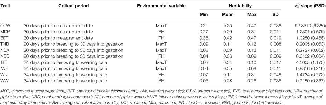
TABLE 3. Description of heritability estimates of each selected environmental variable for each trait.
Considering the traits TNB, NBA, NBD, WN, and WW, RH had the highest σ2a1 estimates for all three of them. For TNB, MaxT had the highest σ2a1 estimate (0.2095) and RH the lowest (0.1042). MaxT was the highest for NBA (0.2727) and DI the lowest (0.0364). The trait NBD had the lowest σ2a1 estimates compared to all the other studied traits, being RH the ENV with the highest σ2a1 (0.0122) and MaxT the lowest (0.0022), showing an opposite trend than TNB. Two critical time periods were evaluated for WN and WW considering 34 days prior to the farrow date (abbreviated as WN_fd and WW_fd, respectively) and 34 days prior to farrowing until weaning date (abbreviated as WN_wd and WW_wd, respectively), resulting in the largest estimates of σ2a1 considering the critical period until weaning date. For WN_fd and WN_wd, RH had the largest σ2a1 estimate (1.291 and 1.473, respectively), while the lowest was DI (0.719) for WN_fd and MaxT (0.4102) for WN_wd. The same pattern of WN was observed for WW, where for WW_fd and WW_wd the largest estimate of σ2a1 came from RH (0.373 and 0.715 kg2, respectively) and the lowest from DI (0.077 kg2) for WW_fd and MaxT (0.046 kg2) for WW_wd. In summary, RH (MDP, BFT, NBD, WN, and WW) and MaxT (OTW, TNB, NBA, IBF, and IWE) were the ENV yielding the highest estimates of the slope term. In addition, for OTW_30, both MaxT and THI could be recommended based on similar results.
Overall, the accuracy of GEBV was greater for the intercept than for the slope term. The largest accuracy for the intercept was observed for BFT_30 considering MaxT (0.7224) as the ENV, and the lowest was for WN_fd considering RH (0.3121) as the ENV. Considering the slope term, the highest accuracy was observed for MaxT (0.6375) in OTW_30 and the lowest was MinT (0.2547) in MDP_120. Within each trait, it was not possible to observe a clear pattern regarding the ranking of ENV, as it was variable depending on the trait analyzed. The accuracy estimates for each trait considering all ENV are shown in Supplementary Table S2, and the accuracy values of the recommended ENV for each trait are shown in Table 4.
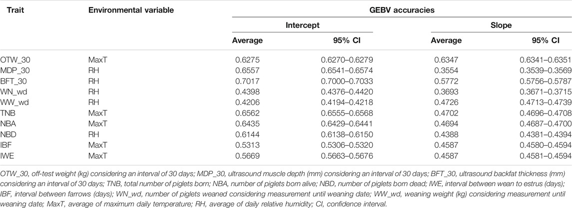
TABLE 4. Accuracies (95% confidence interval) of genomic estimated breeding value for the reaction norm intercept and slope terms considering the recommended environmental variable.
The critical period of 30 days, on average, presented higher accuracies than the critical period of 120 days, on average, for BFT, OTW, and MDP. For BFT_30, the estimated accuracy for the intercept term ranged from 0.6960 (THI) to 0.7161 (DewP), while for the slope it ranged from 0.4118 (DI) to 0.5772 (RH). A different pattern, with lower estimates was observed for BFT_120, ranging from 0.6855 (MaxT) to 0.7151 (MinT) for the intercept and from 0.4153 (MeanT) to 0.4677 (MinT) for the slope. For OTW_30, the accuracy ranged from 0.5985 (RH) to 0.7132 (MaxT) for the intercept and from 0.5562 (DewP) to 0.6375 (MaxT) for the slope term, while OTW_120 ranged from 0.6156 (DewP) to 0.7738 (MaxT) and from 0.4279 (MinT) to 0.0.4909 (THI) for the intercept and slope, respectively. For MDP_30, the accuracy estimates for the intercept were similar between ENV, with 0.6405 (THI) and 0.6629 (MaxT), for the lowest and the highest values, respectively. For the slope term of MDP_30, the accuracy of GEBV ranged from 0.3103 (DI) to 0.3554 (RH). Considering MDP_120, the estimates ranged from 0.6330 (THI) to 0.0.6759 (MaxT) for the intercept and from 0.2547 (MinT) to 0.3209 (RH).
For TNB, NBA, and NBD, the accuracy estimates of GEBV for the intercept and slope terms had similar values between traits and ENV. The accuracy of GEBV for the intercept term ranged from 0.6473 (THI) to 0.6562 (MaxT), from 0.6287 (MeanT) to 0.6463 (MinT), and from 0.6128 (THI) to 0.6239 (MeanT) for TNB, NBA, and NBD, respectively. For the slope, the GEBV accuracies ranged from 0.4201 (MeanT) to 0.4702 (MaxT), from 0.3809 (RH) to 0.4694 (MaxT), and from 0.4090 (MaxT) to 0.4388 (RH) for TNB, NBA, and NBD, respectively. Regarding IBF, GEBV accuracy ranged from 0.4776 (DewP) to 0.5776 (THI) and from 0.3208 (MeanT) to 0.4587 (MaxT) for the intercept and slope terms, respectively. For IWE, the GEBV accuracies ranged from 0.5084 (DI) to 0.4049 (MaxT) and from 0.3372 (MinT) to 0.4587 (MaxT), respectively, for the intercept and slope terms.
Finally, considering the critical period of 34 days prior to farrowing date and 34 days prior to farrowing date until weaning date for WN and WW, respectively, more accurate GEBVs were observed for the intercept term as for the other discussed traits. For WN_fd, GEBV accuracies ranged from 0.3121 (RH) to 0.4710 (DI) and from 0.2735 (MinT) to 0.3475 (RH) for the intercept and slope terms, respectively. For WN_wd, the estimates ranged from 0.3253 (MaxT) to 0.4680 (RH) and from 0.2792 (MinT) to 0.3693 (RH) for the intercept and slope terms, respectively. The only trait with higher GEBV accuracy for the slope than intercept was for WN_fd, where an accuracy of 0.3121 for the intercept and 0.3475 for the slope was observed for RH. Considering WW_fd, the estimated accuracy of GEBV ranged from 0.4144 (THI) to 0.5172 (RH) and from 0.3373 (MaxT) to 0.4126 (RH) for the intercept and slope terms, respectively. For WW_wd, the estimates for the intercept and slope ranged from 0.4215 (MinT) to 0.5895 (THI) and from 0.3703 (MinT) to 0.4726 (RH), respectively. As observed for the first criterion, RH (BFT, MDP, NBD, WN, and WW) and MaxT (IBF and IWE) were the ENV yielding the highest theoretical accuracy of GEBV. For the other traits not previously mentioned, more than one climatic variable could be recommended (RH, THI, and MaxT for OTW, MaxT and RH for TNB, and MaxT and MeanT for NBA).
High GEBV standard deviations in a certain environmental value means that the identification of animals with the highest and lowest genetic values will be more evident. In this regard, the deviation estimates were similar within each value of ENV within trait. The deviation estimate followed a pattern similar to that found for the RN slope and accuracy of GEBV estimates, being the ENV with the largest deviations the same, in most cases, as those that yielded higher σ2a and accuracy results. For OTW_30, OTW_120, TNB, NBA, IBF, and IWE, MaxT yielded the greatest deviation in most of the five categories (each category represents the value allocated in the 0th, 25th, 50th, 75th, and 100th position in each ENV). For the MDP_30, MDP_120, BFT_30, NBD, WN_wd, WN_fd, and WW_wd, the ENV based on RH yielded the higher deviation in most of the ENV values. Lastly, for the remaining traits, there was no absolute ENV that yielded higher deviations. In the case of BFT_120, MaxT, MinT, and DI yielded the highest values, and for WW_fd, the highest values were for RH, MeanT, and MinT. A complete estimation of the deviation in each “ENV × critical period × trait” combination is shown in Supplementary Table S4.
ptA summary of the results of the three criteria presented above is shown in Table 4 as well as the recommended ENV and critical period for each trait. In brief, the critical period of an average of 30 days yielded higher estimates of σ2a and accuracy and deviation of GEBV per ENV. Additionally, the critical period ranging from 34 days prior to farrowing date until weaning date yielded the highest estimation of the three criteria. Moreover, the recommended ENVs for OTW_30 were THI and MaxT, for BFT_30, MDP_30, NBD, WN_wd, and WW_wd was RH, and for TNB, NBA, IBF, and IWE was MaxT. Subsequent results will be presented only for the recommended ENV and critical periods.
The heritability (h2) estimates across the range of the selected ENV for each trait are shown in Table 3 and the complete pattern in Figure 1. The average h2 ranged from 0.04 (IBF) to 0.42 (BFT_30). A similar pattern was observed for TNB (from 0.09 to 0.12), NBA (from 0.08 to 0.12), and NBD (from 0.04 to 0.09), where a slight increase in h2 is observed as the ENV values increase. The traits OTW_30 (from 0.21 to 0.47), WN_wd (from 0.07 to 0.31), and WW_wd (from 0.05 to 0.26) also had a similar pattern, with higher h2 in extreme ENV values and lower estimates closer to the mean. An opposite pattern of average h2 was observed for MDP_30 (from 0.27 to 0.31) and BFT_30 (from 0.38 to 0.47). As the values of ENV increased, the h2 for MDP_30 also increases, and for BFT_30 it decreases. The heritability estimates within each trait (i.e., considering all the ENV and critical periods evaluated) had similar patterns and are shown in Supplementary Table S5.
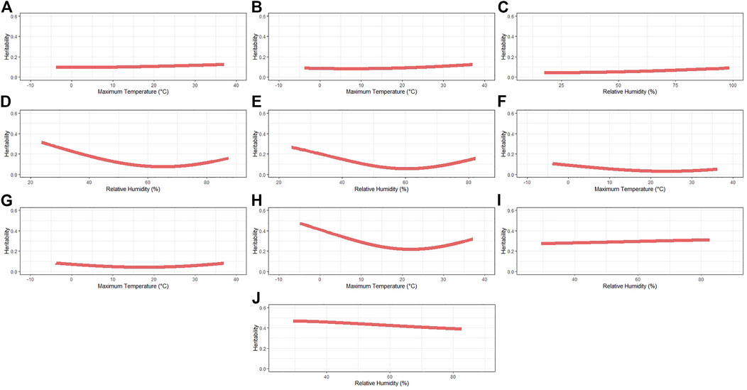
FIGURE 1. Heritability estimates for each recommended environmental variable and critical period for each studied trait. (A) Total number of piglets born. (B) Number of piglets born alive. (C) Number of piglets born dead. (D) Number of piglets weaned considering measurement until weaning date. (E) Weaning weight (kg) considering the measurement of records until weaning date. (F) Interval between wean to estrus (days). (G) Interval between farrows (days). (H) Off-test weight (kg) considering an interval of 30 days. (I) Ultrasound muscle depth (mm) considering an interval of 30 days. (J) Ultrasound backfat thickness (mm) considering an interval of 30 days.
Sires were selected to have at least 30 offspring so that the phenotypes were distributed under a large range in ENV (i.e., records of daughters could not be concentrated under the comfortable environmental gradients). The reaction norms for the slope term of the additive genetic effect of the five most HT and the five most heat-susceptible (HSusc) sires are reported in Figure 2. Re-rankings of animals were clearly observed for NBA, WN_wd, WW_wd, IWE, IBF, and OTW_30, while no clear re-ranking was observed for NBD, MDP_30, and BFT_30. Meanwhile, there was a trend of re-ranking observed for TNB at the best environmental conditions. For TNB (Figure 2A), HT sires appear to have higher performance than the HSusc sires even when the temperature increases. For NBA (Figure 2B), IWE (Figure 2F), IBF (Figure 2G), and OTW_30 (Figure 2H), a clear distinction between groups was observed, with HT sires performing better in the highest temperatures, while the HS performed better in the lower temperatures. For WN_wd (Figure 2D) and WW_wd (Figure 2E), the HT sires were observed to have better performance under environments with higher humidity, while the HSusc sires had a better performance under drier environments. For MDP_30 (Figure 2I) and BFT_30 (Figure 2J), no re-ranking was observed. For all traits, even though some of them do not have a clear re-ranking, it is possible to observe that there are groups of animals performing better than the average population performance (Figure 2, black lines) in challenging environments.
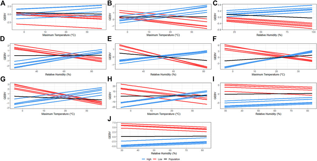
FIGURE 2. Genomic estimated breeding values for each recommended environmental variable and critical period for each studied trait considering five most heat-tolerant and five most heat-susceptible sires. The black line indicates the population trend, the blue lines indicate the most tolerant sires, and the red line indicates the most susceptible sires. (A) Total number of piglets born. (B) Number of piglets born alive. (C) Number of piglets born dead. (D) Number of piglets weaned considering measurement until weaning date. (E) Weaning weight (kg) considering measurement until weaning date. (F) Interval between wean to estrus (days). (G) Interval between farrows (days). (H) Off-test weight (kg) considering an interval of 30 days. (I) Ultrasound muscle depth (mm) considering an interval of 30 days. (J) Ultrasound backfat thickness (mm) considering an interval of 30 days.
In addition, the Spearman (rank) correlations are shown in Supplementary Figure S2 for combinations of intercept and slope terms between each pair of traits. The greatest rank correlations were between TNB and NBA, where between intercepts was equal to 0.917 and between slopes was equal to 0.838, indicating that the GEBV of TNB tends to increase when the GEBV of NBA increases. All other trait combinations had moderate to low rank correlations. Between MDP_30 and OTW_30, IBF and TNB, IBF and NBA, and between MDP_30 and TNB, the slope terms were equal to 0.216, 0.155, 0.188, and 0.113. Negative rank correlations between the slope terms were observed for WN-wd and TNB (−0.196), WN_wd and NBA (−0.185), BFT_30 and WW_wd (−0.149), and IWE and WW_wd (−0.141). The remaining rank correlations between trait combinations for the intercept and slope terms had low rank correlations and are presented in Supplementary Figure S2.
The genetic correlations of additive genetic effects across environmental gradients are shown in Figure 3 (for weak and moderate correlations) and Supplementary Figure S1 (for strong correlations). All estimated genetic correlations between environments considered just ENV values ranging from the 10th to the 90th percentiles, therefore excluding extreme ENV values. The exclusion of the extreme values was done to remove ENV with a low number of records, which might affect the estimation of the parameters at the extremes. As expected, the genetic correlation decreased gradually for greater differences among the environmental gradients. The lowest genetic correlation was observed for WN_wd (Figure 3; average = 0.75), even reaching negative values (-0.274). In addition to WN_wd, IBF (Figure 3; average = 0.79), WW_wd (Figure 3; average = 0.80), and IWE (Figure 3; average = 0.83) seem to be largely affected by G×E interaction. Moderate interactions were observed for OTW_30 (Figure 3; average = 0.88), NBA (Figure 3; average = 0.92), and TNB (Figure 3; average = 0.96). The highest genetic correlations were observed for NBD (Supplementary Figure S1; average = 0.98), MDP_30 (Supplementary Figure S1), and BFT_30 (Supplementary Figure S1), with both of the latter having an average of 0.99. Therefore, we concluded that WN_wd, IBF, WW_wd, and IWE are largely and OTW_30, NBA, and TNB are moderately affected by the G×E interaction. However, NBD, MDP_30, and BFT_30 were only mildly affected by G×E interaction.
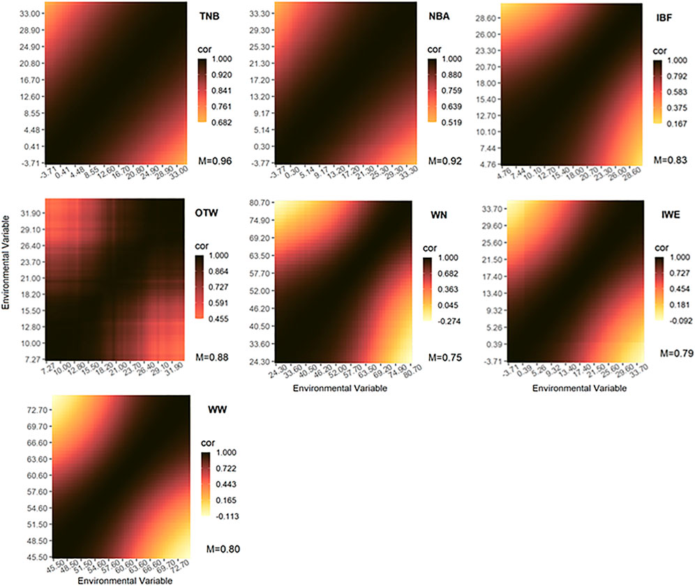
FIGURE 3. Genetic correlations across environmental gradients using the recommended environmental variable and critical period for each studied trait. The Pearson correlation coefficient (cor) are represented by colors with the mean values shown below. TNB, total number of piglets born; NBA, number of piglets born alive; WN, number of piglets weaned considering the measurement of records until weaning date; WW, weaning weight (kg) considering measurement until weaning date; IWE, interval between wean to estrus (days); IBF, interval between farrows (days); OTW, off-test weight (kg) considering an interval of 30 days.
Individuals with GEBV theoretical accuracies higher than 0.30 were used to calculate the weighted Pearson correlation among the RN intercepts and slopes between all studied traits considering the recommended ENV for each trait. The minimum number of selected animals and the lowest average accuracies were 5,718 and 0.4224 (95% CI of 0.4210–0.4236), respectively (Supplementary Table S6). The approximate genetic correlations between intercepts, intercept and slope, slope and intercept, and slope and slope for each pair of traits (considering the recommended ENV for each trait) are shown in Figure 4.
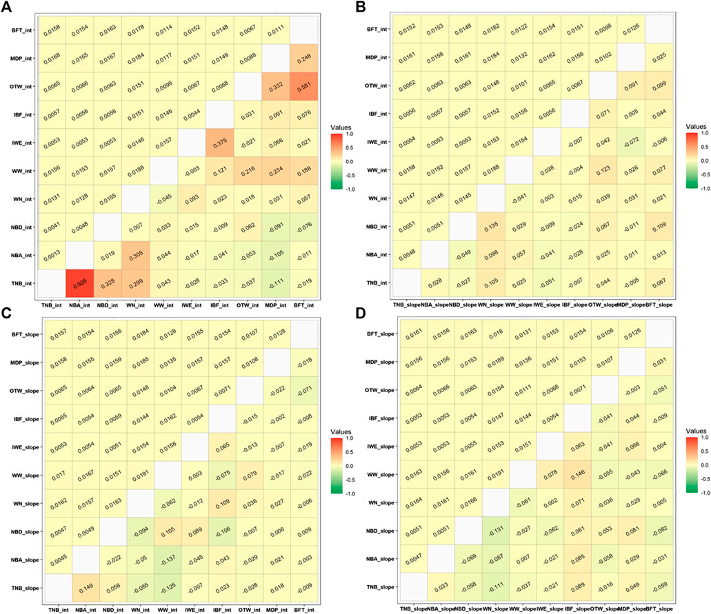
FIGURE 4. Approximated Pearson genetic correlations (lower) and standard errors (upper) among (A) intercept terms, (B) intercept and slope, (C) slope and intercept, and (D) slope terms of the recommended environmental variable and critical period for each studied trait. TNB, total number of piglets born; NBA, number of piglets born alive; NBD, number of piglets born dead; WN, number of piglets weaned; WW, weaning weight (kg); IWE, interval between wean to estrus (days); IBF, interval between farrows (days); OTW, off-test weight (kg); MDP, ultrasound muscle depth (mm); BFT, ultrasound backfat thickness (mm). For OTW, MDP, and BFT, we considered a critical period of an average of 30 days before measurement date. For WN and WW, we considered a critical period from 34 days prior to farrowing up to weaning date. For TNB, NBA, and NBD, we considered a critical period of 20 days prior to breeding to 30 days into gestation. For IBF and IWE, we considered a critical period of 34 days prior to farrowing to weaning date.
The greatest genetic correlations were observed between the intercept terms. The greatest positive correlations were observed between TNB and NBA, with 0.928, and between BFT_30 and OTW_30 (0.581) for the RN intercept. A moderate genetic correlation was also observed between TNB and NBD (0.328), TNB and WN_wd (0.305), and NBA and WN_wd (0.305). Moderate genetic correlations between intercepts were also observed between IBF and IWE (0.375), MDP_30 and OTW_30 (0.332), and BFT_30 and MDP_30 (0.248). For WW_wd, moderate to low genetic correlations were observed with IBF (0.121), OTW_30 (0.216), MDP_30 (0.234), and BFT_30 (0.188). The combinations for the remaining traits for the intercept term had low genetic correlations and are shown in Figure 4A.
Approximate genetic correlations between the intercept and slope terms indicate what happens to the performance of an animal for a specific trait when another trait is expressed under challenging heat conditions. In this matter, the greatest positive correlation was between TNB slope and NBA intercept (0.149) and between NBD intercept and WN slope (0.135). A similar positive correlation was also observed between WW intercept and OTW slope (0.123) and between the pairs of BFT slope with NBD intercept and IBF intercept with WN slope (both equal to 0.109). The WN slope and TNB intercept and the NBD slope and WW intercept had the same correlation value of 0.105. The greatest negative correlation was observed between the NBA slope and the TNB slope with WW intercept (−0.137 and −0.125, respectively). All other combinations between intercept and slope had values lower than 0.100 (Figure 4B,C).
The smallest genetic correlations were observed between the slope terms. This correlation indicates the relationship between the traits under a stressful environmental condition. The greatest positive slope × slope genetic correlation was observed for WW_wd and IBF (0.146). A negative correlation of -0.131 was observed for NBD and WN_wd and of -0.111 between WN_wd and TNB. All the other trait combinations had correlations under the absolute value of 0.100 and are shown in Figure 4D.
A set of comprehensive analyses to reveal the genetic background of HTol based on routinely measured phenotypic records and publicly recorded weather variables was performed in this study.
As indicated in the “Materials and Methods” section, three different metrics were used as criteria for the selection and recommendation of ENV and critical period to evaluate HTol in pigs from the Large White breed (one of the main maternal-line breeds). The first criterion, based on the ENV yielding the higher G×E interaction measured by the σ2a1 term, was also used by other studies evaluating HS effects in reproductive and carcass traits in pure breeds and crossbred animals (Tiezzi et al., 2020; Usala et al., 2021). The second criterion was based on the theoretical accuracy of GEBV. Therefore, the climatic metric recommended had to not only have the strongest G×E but also provide more reliable GEBV estimates. Furthermore, the third criterion was based on the ENV yielding the greatest deviation of GEBV within the ENV value. The latest mentioned criterion was considered because, in this study, the goal was to use an ENV that allows a clear distinction (i.e., higher dispersion of breeding values) between HT and HSusc animals. A large variability in GEBV (i.e., higher standard deviation of GEBV within each ENV value) allows better discrimination of the animals, which facilitates the selection of the desired animals. Another metric that could also be evaluated was the deviance information criterion (DIC). However, in this study, the DIC was not included as another criteria for ENV selection due to criticisms found in the literature, such as the lack of consistency, weak theoretical justification, and overfitting (Spiegelhalter et al., 2014; Clarke and Clarke, 2018; Salles et al., 2019).
Climate records from the National Climatic Data Center weather stations were used to describe the environmental conditions experienced by the sows at different stages of ovulation, pregnancy, and post-pregnancy. Weather stations used in the current study were on average within 30 km from the farm. Freitas et al. (2006) estimated a correlation of 0.9 between on-farm weather data and weather station data even for weather stations more than 300 km away from the farm. Although these climate records are usually publicly available and have been successfully used in other worldwide studies focusing on sow HTol for different reproduction, growth, and carcass traits (Tummaruk et al., 2010; Wegner et al., 2014; Tiezzi et al., 2020; Usala et al., 2021), we acknowledge that the collection of within-barn environmental measurements is important and should be done when possible. However, the variables needed for this study were not available for this current study. It is also worth noting that, although there was a large variability in the climatic variables used in this study, they might not be representative of all the possible range of climatic conditions. Therefore, additional studies should be performed in other populations (e.g., breeds) and geographical regions to confirm our results.
In the current study, acute HS had greater impact on OTW, BFT, and MDP than chronic HS, which suggests that, during the period of chronic HS, the animal might be able to recover from the thermal stress suffered. For these traits (OTW, BFT, and MDP), the variance components for the slope term were higher considering a period of 30 days before measurement than 120 days. The GEBV accuracy estimates were also greater for the acute HS. For WW and WN, the period ranging from the last stage of gestation (around day 80) until the weaning date resulted in higher G×E interaction and GEBV accuracies. Therefore, the time period ranging from the last stage of gestation until weaning date is the recommended critical period to evaluate HT for WW and WN (referred here as WW_wd and WN_wd, respectively).
Several studies implemented different climatic variables as the environmental gradient covariate—for instance, some studies used heat load calculated as THI greater than 70, temperature, humidity, or THI (Fragomeni et al., 2016; Tiezzi et al., 2020; Usala et al., 2021). However, reports of the best environmental metric to be used when evaluating HTol in pigs from the maternal line are scarce. Therefore, we evaluated several ENV based on temperature and humidity to achieve a recommendation for each of the evaluated traits. The use of an index-based environmental variable is another way of carrying out the analyses, and it has been done in plants (e.g., Resende et al., 2020). However, in the current study, single ENV was used as environmental gradient. The use of RH as the climatic variable is the recommendation for NBD, WW_wd, WN_wd, MDP_30, and BFT_30. Maximum temperature is the recommended ENV for TNB, NBA, IBF, IWE, and OTW_30. Even though for OTW_30 the use of MaxT was recommended based on our findings, THI also resulted in a very similar G×E interaction. This choice was based on THI development as most THI are originally related to the body temperatures of cattle exposed to HS and have been adapted to other species or populations (Ingraham et al., 1979; Buffington et al., 1981; Bohmanova et al., 2007). Therefore, the use of THI in pigs is viewed with caution since different physiological and anatomical characteristics (i.e., rumen, ability to sweat, body mass, etc.) are found between cattle and swine that directly influence thermotolerance. For OTW, a high (0.79) rank correlation between GEBV estimates using THI and MaxT was observed. Therefore, due to the caution in interpreting the THI values for swine and the high rank correlation between THI with MaxT, MaxT was recommended as the ENV to evaluate HTol in maternal-line pigs for OTW. For five out of the 10 traits evaluated, the ENV selected (Table 5) were built upon RH as climate variable and the other five used MaxT. The preponderance of RH, rather than other climatic variables, in challenged sows was reported by Tummaruk et al. (2010) and Tiezzi et al. (2020) who studied reproductive performance under HS conditions. This finding might indicate that the barn cooling systems can better mitigate the impact of temperature than RH.
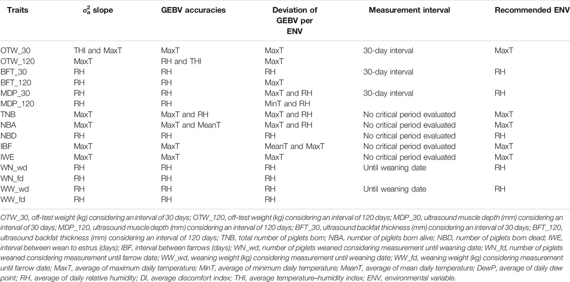
TABLE 5. Summary and recommendation of the three criteria evaluated of each environmental variable for each trait.
Genomic RNM were used in this study for the estimation of genetic parameters, including additive genetic variance for the trait performance in a standard environment (σ2a0, intercept term) as well as the additive genetic variance for the tolerance to a given environmental stressor (σ2a1, slope term). The additive genetic variance estimates obtained agree with the estimates by Chen et al. (2021) when evaluating HT based on CGe in the same population. The heritability estimates are in the same range with the ones reported by Tiezzi et al. (2020), using the average RH before conception (for TNB) or the average THI index during the pregnancy of sows (for NBA). Chen et al. (2021), using CGe, also found a similar h2 for TNB, NBA, WW, and MDP. A higher average h2 for NW was estimated using RH as the environmental gradient when compared to CGe (Chen et al., 2021).
As described by Usala et al. (2021), the use of RNM to assess the environmental effect on animal fertility, conformation, or carcass quality traits is less common in pigs when compared to dairy and beef cattle (Meyer, 2000; Coffey et al., 2002; Bradford et al., 2016; Ansari-Mahyari et al., 2019). In pigs, the genetic component for HTol is usually calculated as a function of heat load on growth traits or carcass weight (Zumbach et al., 2008; Fragomeni et al., 2016). Estimating genetic parameters for HTol in crossbred swine carcass traits, Usala et al. (2021) also observed a high average h2 for BFT and MDP. The heritability estimated for the beginning of the curve (assumed as a comfortable condition compared to the right extreme values) was also a trend observed by Tiezzi et al. (2020) for TNB and NBA. Silva et al. (2014) also reported a higher h2 for TNB in contemporary groups with better performance, and a similar trend was observed by Fragomeni et al. (2016) when assessing HTol based on the body weight of purebred Duroc individuals. The use of quadratic functions is another alternative to analyze the data. However, considering the biological aspect of heat stress, the use of quadratic or higher-order functions can compromise the interpretation of results (e.g., using a quadratic function could mean that, when temperature increases, the impact of heat stress would be higher, but after a certain point, this impact would be favorable even though the temperature continues to increase).
The most common thresholds recommended for considering the presence of G×E interaction are based on genetic correlations across the range of ENV lower than 0.70 (Mulder and Bijma, 2007) or 0.80 (Hayes et al., 2016). In this study, only NW, WW, and IBF presented a G×E interaction considering an average threshold of 0.80. However, despite the fact that some traits had an average correlation value higher than the threshold correlation of 0.80, the minimum values found for TNB, NBA, IWE, and OTW were lower than this threshold. Therefore, we suggest that moderate G×E interactions were observed in such traits. For NBD, MDP, and BFT, both average and minimum values are above the 0.80 threshold, indicating a low G×E interaction across ENV values, which is also supported by the RN of GEBV for the mentioned traits (Figures 2C,I,J). Similar values of genetic correlations across ENV were found by Tiezzi et al. (2020) for TNB and NBA, in which the correlation between RH values reached 0.78 and that between THI reaching 0.83, respectively. Additionally, Chen et al. (2021) observed similar average values when considering CGe as the environmental covariate for BFT. However, differently from Chen et al. (2021), in the current study, stronger G×E interactions were observed for WN and moderate for OTW. Usala et al. (2021) observed lower values for the genetic correlations in crossbred animals (0.89 and 0.50 for BFT and loin depth, respectively, using RH). These results suggest that the G×E interaction is not only population dependent but also dependent on the environmental covariate used. It is important to note that the estimates of G×E might not reflect the exact environmental conditions experienced by the animals because public weather station data may not precisely represent within-barn environmental conditions. Therefore, further studies should consider in-barn recorded environmental data to validate the results.
Visualizing more HT animals can be facilitated using RN plots (Figure 2). Individuals with better performance under HS conditions can be selected and used within a breeding scheme, provided that they are not under-performing under thermoneutral conditions (i.e., comfortable and controlled climatic conditions). Except for TNB, NBD, MDP, and BFT, the best-performing animals under challenging environmental conditions (i.e., high humidity or temperature) are under-performing in comfortable conditions. The identification of these animals (or their descendants) means that the use of their genetic resources will be better applied on farms experiencing high RH or temperature values. For TNB and NBD, the most HT animals performed better under both comfortable and challenging conditions, and the opposite trend occurred with MDP and BFT, where the more HSusc animals outperformed the most HT across the entire ENV range. These results agree with the G×E interaction (Figures 3C,I,J), where high correlations were found for NBD, MDP, and BFT.
The highest positive genetic correlations observed between TNB and NBA intercept terms were also observed by Serenius et al. (2004) in Finnish Large White pigs. Serenius et al. (2004) estimated the genetic correlation for first farrowing interval with TNB, NBA, and WN to be higher (0.130, 0.160, and 0.140, respectively) than the values found in this study, where the correlation between IBF intercept and TNB, NBA, and WN intercept had negative values (−0.033, −0.041, and −0.009). Moderate correlations between OTW, MDP, and BFT were observed in this study and were also reported by Chen et al. (2021) and Jiao et al. (2014). The genetic correlations among slopes for different traits were low to moderate, which indicate that HTol based on different traits could result in the selection of different animals. These results are important to the industry as they indicate that pigs should be selected for HTol defined based on multiple traits and potentially combined in a selection sub-index. However, as there are no gold-standard values (e.g., true breeding values), the fact that the breeding values for HTol based on alternative traits are different or that re-ranking occurred cannot be used for choosing the best environmental variable for each trait. In addition, the fact that these correlations between slopes are low to moderate indicates the need to evaluate traits in different environments. These findings contribute to improving selection strategies under HT and suggest that different animals would be selected depending on the trait evaluated. Selection can be achieved by selecting for all traits, especially when including the traits in a selection sub-index, according to the desired breeding goal.
Different environmental gradients for the RN have been used over time (CGe: Li and Hermesch, 2016; Song et al., 2020; Chen et al., 2021 and climatic variables: Fragomeni et al., 2016; Tiezzi et al., 2020; Usala et al., 2021). However, the feasibility of using the average CGe or climatic variables as the environmental gradient for assessing G×E interactions is unknown. In this regard, Chen et al. (2021), using the same population and seven traits also used in the current study (OTW, MDP, BFT, TNB, NBA, WN, and WW), calculated the GEBV of animals using CGe as the environmental gradient. In general, the estimates based on the recommended ENV of the current study resulted in higher theoretical accuracies of GEBV, except for MDP, where the accuracy based on CGe was 0.580 (i.e., indicator of G×E interaction), while the accuracy based on the recommended ENV was 0.350 for the slope term. A Spearman (rank) correlation between the GEBV of individuals regressed on the recommended ENV and CGe shows a negative moderate rank correlation for BFT (−0.57), WW (−0.47), and MDP (−0.31) and a low positive rank correlation for the other traits (Supplementary Table S7). These results suggest that, despite being used and historically providing reliable breeding value estimates (Song et al., 2020; Chen et al., 2021), the use of CGe accounts for additional variability, including nutrition practices and management. This might not be the interest when evaluating HTol. Therefore, as suggested, the use of ENV might be more useful when the objective is to evaluate the breeding values of animals under challenging climatic stress.
The genetic and genomic background of HTol was comprehensively explored in the present study for various reproduction, growth, and body composition traits measured in pigs from the Large White breed (maternal line). Moreover, the use of different critical periods and climatic variables defined based on public weather station records was evaluated. Our results indicate that evaluating HS in the period of 30 days before the measurement date provided the best estimates of G×E for OTW, MDP, and BFT. Additionally, the critical period ranging from the last trimester of gestation until weaning provided better estimates for WN and WW. From the climatic variables evaluated, the average RH (for NBD, WN, WW, MDP, and BFT) and MaxT (for TNB, NBA, IWE, IBF, and OTW) are the recommended variables to evaluate HS based on the mentioned traits. Large (WN, WW, IBF, and IWE) and moderate (OTW, TNB, and NBA) G×E interactions were observed for most of the studied traits, while other traits (MDP, BFT, and NBD) are less impacted by heat stress, showing a weaker evidence of G×E. The low to moderate genetic correlations between HTol breeding values based on different traits indicate that a selection sub-index combining the breeding values for the slopes of multiple traits might be needed for identifying the most HT animals throughout their entire productive life. The current study also demonstrates that HTol is heritable, and genetic progress can be achieved through direct genetic and genomic selection. Therefore, selecting for improved HTol based on reproductive, growth, and body composition performance and public weather station data is feasible in swine. Future research using within-barn environmental records will be performed next.
The data analyzed in this study is subject to the following licenses/restrictions: The phenotypic and genomic data used in this study are a property of the industry partner that contributed to the study and therefore are not readily available due to its commercially sensitivity. Requests to access these datasets should be directed to Yijian Huang, yhuang@smithfield.com.
Ethical review and approval was not required for the animal study because all the datasets used were provided by commercial breeding operations.
LB, JJ, FT, and AS conceived and designed this research. LB provided training to the first author and coordinated the project. PF performed the data analyses with the assistance of SC, HO, SL, and LB. PF wrote the initial version of the manuscript. YH and YG provided all the datasets, technical assistance, and suggestions in the final version of the manuscript. All authors interpreted the results, edited the manuscript, and approved the final version of the manuscript.
This work was funded by the Agriculture and Food Research Initiative Competitive Grant number 2020-67015-31575 from the USDA National Institute of Food and Agriculture.
YH and YG were employed by Smithfield Premium Genetics.
The remaining authors declare that the research was conducted in the absence of any commercial or financial relationships that could be construed as a potential conflict of interest.
All claims expressed in this article are solely those of the authors and do not necessarily represent those of their affiliated organizations or those of the publisher, the editors, and the reviewers. Any product that may be evaluated in this article or claim that may be made by its manufacturer is not guaranteed or endorsed by the publisher.
We acknowledge the phenotypic, pedigree, and genomic datasets provided by the Smithfield Premium Genetics (Raleigh, NC, United States of America) breeding company.
The Supplementary Material for this article can be found online at: https://www.frontiersin.org/articles/10.3389/fgene.2021.717409/full#supplementary-material.
Aguilar, I., Fernandez, E. N., Blasco, A., Ravagnolo, O., and Legarra, A. (2020). Effects of Ignoring Inbreeding in Model‐based Accuracy for BLUP and SSGBLUP. J. Anim. Breed. Genet. 137, 356–364. doi:10.1111/jbg.12470
Aguilar, I., Misztal, I., Johnson, D. L., Legarra, A., Tsuruta, S., and Lawlor, T. J. (2010). Hot Topic: A Unified Approach to Utilize Phenotypic, Full Pedigree, and Genomic Information for Genetic Evaluation of Holstein Final Score. J. Dairy Sci. 93, 743–752. doi:10.3168/jds.2009-2730
Akaike, H. (1973). “Information Theory and an Extension of the Maximumlikelihood Principle,” in Proceedings of 2nd International Symposium on Information Theory (Budapest, Hungary: IEEE), 267–281.
Almeida-de-Macedo, M. M., Ransom, N., Feng, Y., Hurst, J., and Wurtele, E. S. (2013). Comprehensive Analysis of Correlation Coefficients Estimated from Pooling Heterogeneous Microarray Data. BMC Bioinformatics 14, 214. doi:10.1186/1471-2105-14-214
Ansari-Mahyari, S., Ojali, M. R., Forutan, M., Riasi, A., and Brito, L. F. (2019). Investigating the Genetic Architecture of conception and Non-return Rates in Holstein Cattle under Heat Stress Conditions. Trop. Anim. Health Prod. 51, 1847–1853. doi:10.1007/s11250-019-01875-5
Baumgard, L. H., and Rhoads, R. P. (2013). Effects of Heat Stress on Postabsorptive Metabolism and Energetics. Annu. Rev. Anim. Biosci. 1, 311–337. doi:10.1146/annurev-animal-031412-103644
Bernabucci, U. (2019). Climate Change: Impact on Livestock and How Can We Adapt. Anim. Front. 9, 3–5. doi:10.1093/af/vfy039
Bohmanova, J., Misztal, I., and Cole, J. B. (2007). Temperature-Humidity Indices as Indicators of Milk Production Losses Due to Heat Stress. J. Dairy Sci. 90, 1947–1956. doi:10.3168/jds.2006-513
Bradford, H. L., Fragomeni, B. O., Bertrand, J. K., Lourenco, D. A. L., and Misztal, I. (2016). Genetic Evaluations for Growth Heat Tolerance in Angus Cattle1. J. Anim. Sci. 94, 4143–4150. doi:10.2527/jas.2016-0707
Buffington, D. E., Collazo-Arocho, A., Canton, G. H., Pitt, D., Thatcher, W. W., and Collier, R. J. (1981). Black Globe-Humidity Index (BGHI) as Comfort Equation for Dairy Cows. Trans. ASAE 24, 0711–0714. doi:10.13031/2013.34325
Cabezón, F. A., Schinckel, A. P., Richert, B. T., Stewart, K. R., Gandarillas, M., and Peralta, W. A. (2016). Analysis of Lactation Feed Intakes for Sows Including Data on Environmental Temperatures and Humidity. The Prof. Anim. Scientist 32, 333–345. doi:10.15232/pas.2015-01495
Carabaño, M. J., Ramón, M., Díaz, C., Molina, A., Pérez-Guzmán, M. D., and Serradilla, J. M. (2017). Breeding and Genetics Symposium: Breeding for Resilience to Heat Stress Effects in Dairy Ruminants. A Comprehensive Review. J. Anim. Sci. 95, 1813–1826. doi:10.2527/jas2016.1114
Chen, S.-Y., Freitas, P. H. F., Oliveira, H. R., Lázaro, S. F., Huang, Y. J., Howard, J. T., et al. (2021). Genotype-by-environment Interactions for Reproduction, Body Composition, and Growth Traits in Maternal-Line Pigs Based on Single-step Genomic Reaction Norms. Genet. Sel. Evol. 53, 51. doi:10.1186/s12711-021-00645-y
Christensen, O. F., and Lund, M. S. (2010). Genomic Prediction when Some Animals Are Not Genotyped. Genet. Sel. Evol. 42, 2. doi:10.1186/1297-9686-42-2
Clarke, B., and Clarke, J. (2018). Predictive Statistics: Analysis and Inference beyond Models Cambridge Series in Statistical and Probabilistic Mathematics. Cambridge: Cambridge University Press.
Coffey, M. P., Simm, G., and Brotherstone, S. (2002). Energy Balance Profiles for the First Three Lactations of Dairy Cows Estimated Using Random Regression. J. Dairy Sci. 85, 2669–2678. doi:10.3168/jds.s0022-0302(02)74352-x
Edwards, R. L., Omtvedt, I. T., Tuesman, E. J., Stephens, D. F., and Mahoney, G. W. (1968). Reproductive Performance of Gilts Following Heat Stress Prior to Breeding and in Early Gestation. Anim. Sci. J. 27, 1634. doi:10.2527/jas1968.2761634x
Fragomeni, B. O., Lourenco, D. A. L., Tsuruta, S., Bradford, H. L., Gray, K. A., Huang, Y., et al. (2016). Using Single-step Genomic Best Linear Unbiased Predictor to Enhance the Mitigation of Seasonal Losses Due to Heat Stress in Pigs. J. Anim. Sci. 94, 5004–5013. doi:10.2527/jas.2016-0820
Freitas, M. S., Misztal, I., Bohmanova, J., and West, J. (2006). Utility of on- and Off-Farm Weather Records for Studies in Genetics of Heat Tolerance. Livestock Sci. 105, 223–228. doi:10.1016/j.livsci.2006.06.011
Gonzalez-Rivas, P. A., Chauhan, S. S., Ha, M., Fegan, N., Dunshea, F. R., and Warner, R. D. (2020). Effects of Heat Stress on Animal Physiology, Metabolism, and Meat Quality: A Review. Meat Sci. 162, 108025. doi:10.1016/j.meatsci.2019.108025
Hayes, B. J., Daetwyler, H. D., and Goddard, M. E. (2016). Models for Genome × Environment Interaction: Examples in Livestock. Crop Sci. 56, 2251–2259. doi:10.2135/cropsci2015.07.0451
Ingraham, R. H., Stanley, R. W., and Wagner, W. C. (1979). Seasonal Effects of Tropical Climate on Shaded and Nonshaded Cows as Measured by Rectal Temperature, Adrenal Cortex Hormones, Thyroid Hormone, and Milk Production. Am. J. Vet. Res. 40 (12), 1792–1797.
Jiao, S., Maltecca, C., Gray, K. A., and Cassady, J. P. (2014). Feed Intake, Average Daily Gain, Feed Efficiency, and Real-Time Ultrasound Traits in Duroc Pigs: I. Genetic Parameter Estimation and Accuracy of Genomic Prediction. J. Anim. Sci. 92 (6), 2377–2386. doi:10.2527/jas.2013-7338
Johnson, J. S., Abuajamieh, M., Sanz Fernandez, M. V., Seibert, J. T., Stoakes, S. K., Nteeba, J., et al. (2015). Thermal Stress Alters Postabsorptive Metabolism during Pre- and Postnatal Development. Clim. Change Impact Livestock: Adaptation Mitigation 1, 61–79. doi:10.1007/978-81-322-2265-1_5
Johnson, J. S., Stewart, K. R., Safranski, T. J., Ross, J. W., and Baumgard, L. H. (2020). In Utero heat Stress Alters Postnatal Phenotypes in Swine. Theriogenology 154, 110–119. doi:10.1016/j.theriogenology.2020.05.013
Kemp, B., Da Silva, C. L. A., and Soede, N. M. (2018). Recent Advances in Pig Reproduction: Focus on Impact of Genetic Selection for Female Fertility. Reprod. Dom Anim. 53, 28–36. doi:10.1111/rda.13264
Kirkpatrick, M., Lofsvold, D., and Bulmer, M. (1990). Analysis of the Inheritance, Selection and Evolution of Growth Trajectories. Genetics 124, 979–993. doi:10.1093/genetics/124.4.979
Li, L., and Hermesch, S. (2016). Evaluation of Sire by Environment Interactions for Growth Rate and Backfat Depth Using Reaction Norm Models in Pigs. J. Anim. Breed. Genet. 133, 429–440. doi:10.1111/jbg.12207
Maskal, J. M., Duttlinger, A. W., Kpodo, K. R., McConn, B. R., Byrd, C. J., Richert, B. T., et al. (2020). Evaluation and Mitigation of the Effects of In Utero Heat Stress on Piglet Growth Performance, Postabsorptive Metabolism, and Stress Response Following Weaning and Transport. J. Anim. Sci. 98 (9), skaa265. doi:10.1093/jas/skaa265
Masuda, Y. (2018). Introduction to BLUPF90 Suite Programs. University of Georgia. Available at: http://nce.ads.uga.edu/wiki/doku.php?id=documentation.
Mayorga, E. J., Renaudeau, D., Ramirez, B. C., Ross, J. W., and Baumgard, L. H. (2018). Heat Stress Adaptations in Pigs. Anim. Front. 9, 54–61. doi:10.1093/af/vfy035
Mayorga, E. J., Ross, J. W., Keating, A. F., Rhoads, R. P., and Baumgard, L. H. (2020). Biology of Heat Stress; the Nexus between Intestinal Hyperpermeability and Swine Reproduction. Theriogenology 154, 73–83. doi:10.1016/j.theriogenology.2020.05.023
Meyer, K. (2000). Random Regressions to Model Phenotypic Variation in Monthly Weights of Australian Beef Cows. Livestock Prod. Sci. 65, 19–38. doi:10.1016/s0301-6226(99)00183-9
Misztal, I. (2017). Breeding and Genetics Symposium: Resilience and Lessons From Studies in Genetics of Heat Stress. J. Anim. Sci. 95, 1780–1787. doi:10.2527/jas2016.0953
Misztal, I., Tsuruta, S., Lourenco, D. A. L., Masuda, Y., Aguilar, I., Legarra, A., et al. (2018). Manual for BLUPF90 Family Programs. University of Georgia. Available at: http://nce.ads.uga.edu/wiki/doku.php?id=documentation.
Misztal, I., Legarra, A., and Aguilar, I. (2009). Computing Procedures for Genetic Evaluation Including Phenotypic, Full Pedigree, and Genomic Information. J. Dairy Sci. 92, 4648–4655. doi:10.3168/jds.2009-2064
Misztal, I., Tsuruta, S., Strabel, T., Auvray, B., Druet, T., and Lee, D. (2002). “BLUPF90 and Related Programs (BGF90),” in Proc. 7th World Congr. Genet. Appl. Livest. Prod (Montpellier, France: IEEE), 21–22.
Mulder, H. A., and Bijma, P. (2007). Effects of Genotype X Environment Interaction on Genetic Gain in Breeding Programs. J. Anim. Sci. 83, 49–61. doi:10.2527/2005.83149x
Omtvedt, I. T., Nelson, R. E., Edwards, R. L., Stephens, D. F., and Turman, E. J. (1971). Influence of Heat Stress During Early, Mid and Late Pregnancy of Gilts. Anim. Sci. J. 32, 312–317. doi:10.2527/jas1971.322312x
R Core Team (2020). R: A Language and Environment for Statistical Computing. Vienna, Austria: R Foundation for Statistical Computing. Available at: https://www.R-project.org/.
Raftery, A. L., and Lewis, S. (1992). Comment: One Long Run with Diagnostics: Implementation Strategies for Markov Chain Monte Carlo. Stat. Sci. 7, 493–497. doi:10.1214/ss/1177011143
Rauw, W. M., and Gomez-Raya, L. (2015). Genotype by Environment Interaction and Breeding for Robustness in Livestock. Front. Genet. 6, 310. doi:10.3389/fgene.2015.00310
Renaudeau, D., Collin, A., Yahav, S., de Basilio, V., Gourdine, J. L., and Collier, R. J. (2012). Adaptation to Hot Climate and Strategies to Alleviate Heat Stress in Livestock Production. Animal 6, 707–728. doi:10.1017/s1751731111002448
Resende, R. T., Piepho, H.-P., Rosa, G. J. M., Silva-Junior, O. B., e Silva, F. F., de Resende, M. D. V., et al. (2020). Enviromics in Breeding: Applications and Perspectives on Envirotypic-Assisted Selection. Theor. Appl. Genet. 134, 95–112. doi:10.1007/s00122-020-03684-z
Salles, O. C., Almany, G. R., Berumen, M. L., Jones, G. P., Saenz‐Agudelo, P., Srinivasan, M., et al. (2019). Strong Habitat and Weak Genetic Effects Shape the Lifetime Reproductive success in a Wild Clownfish Population. Ecol. Lett. 23, 265–273. doi:10.1111/ele.13428
Sargolzaei, M., Chesnais, J. P., and Schenkel, F. S. (2014). A New Approach for Efficient Genotype Imputation Using Information from Relatives. BMC Genomics 15, 478. doi:10.1186/1471-2164-15-478
Serenius, T., Sevón-aimonen, M.-l., Kause, A., Mäntysaari, E. A., and Mäki-tanila, A. (2004). Selection Potential of Different Prolificacy Traits in the Finnish Landrace and Large white Populations. Acta Agriculturae Scand. Section A - Anim. Sci. 54, 36–43. doi:10.1080/09064700310019082
Silva, F. F., Guimarães, S. E. F., Lopes, P. S., Mulder, H. A., Bastiaansen, J. W. M., Knol, E. F., et al. (2014). Sire Evaluation for Total Nnumber Born in Pigs Using a Genomic Reaction Norms Approach. J. Anim. Sci. 92, 3825–3834. doi:10.2527/jas.2013-6486
Smith, B. J. (2007). boa: An R Package for MCMC Output Convergence Assessment and Posterior Inference. J. Stat. Softw. 21, 1–37. doi:10.18637/jss.v021.i11
Song, H., Zhang, Q., Misztal, I., and Ding, X. (2020). Genomic Prediction of Growth Traits for Pigs in the Presence of Genotype by Environment Interactions Using Single‐step Genomic Reaction Norm Model. J. Anim. Breed. Genet. 137, 523–534. doi:10.1111/jbg.12499
Spiegelhalter, D. J., Best, N. G., Carlin, B. P., and Van der Linde, A. (2014). The Deviance Information Criterion: 12 Years on. J. R. Stat. Soc. B 76 (3), 485–493. doi:10.1111/rssb.12062
Stinn, J. P., and Xin, H. (2014). Heat and Moisture Production Rates of a Modern U.S. Swine Breeding, Gestation and Farrowing Facility. Trans. ASABE 57, 1517–1528. doi:10.13031/trans.57.10711
Tiezzi, F., Brito, L. F., Howard, J., Huang, Y. J., Gray, K., Schwab, C., et al. (2020). Genomics of Heat Tolerance in Reproductive Performance Investigated in Four Independent Maternal Lines of Pigs. Front. Genet. 11, 629. doi:10.3389/fgene.2020.00629
Tummaruk, P., Tantasuparuk, W., Techakumphu, M., and Kunavongkrit, A. (2010). Seasonal Influences on the Litter Size at Birth of Pigs Are More Pronounced in the Gilt Than Sow Litters. J. Agric. Sci. 148, 421–432. doi:10.1017/s0021859610000110
Usala, M., Macciotta, N. P. P., Bergamaschi, M., Maltecca, C., Fix, J., Schwab, C., et al. (2021). Genetic Parameters for Tolerance to Heat Stress in Crossbred Swine Carcass Traits. Front. Genet. 11, 612815. doi:10.3389/fgene.2020.612815
VanRaden, P. M. (2008). Efficient Methods to Compute Genomic Predictions. J. Dairy Sci. 91, 4414–4423. doi:10.3168/jds.2007-0980
Vilas Boas Ribeiro, B. P., Lanferdini, E., Palencia, J. Y. P., Lemes, M. A. G., Teixeira de Abreu, M. L., de Souza Cantarelli, V., et al. (2018). Heat Negatively Affects Lactating Swine: A Meta-Analysis. J. Therm. Biol. 74, 325–330. doi:10.1016/j.jtherbio.2018.04.015
Wegner, K., Lambertz, C., Daş, G., Reiner, G., and Gauly, M. (2014). Climatic Effects on Sow Fertility and Piglet Survival Under Influence of a Moderate Climate. Animal 8, 1526–1533. doi:10.1017/S1751731114001219
Wildt, D. E., Riegle, G. D., and Dukelow, W. R. (1975). Physiological Temperature Response and Embryonic Mortality in Stressed Swine. Am. J. Physiol.-Legacy Content 229, 1471–1475. doi:10.1152/ajplegacy.1975.229.6.1471
Williams, A. M., Safranski, T. J., Spiers, D. E., Eichen, P. A., Coate, E. A., and Lucy, M. C. (2013). Effects of a Controlled Heat Stress during Late Gestation, Lactation, and after Weaning on Thermoregulation, Metabolism, and Reproduction of Primiparous Sows1. J. Anim. Sci. 91, 2700–2714. doi:10.2527/jas.2012-6055
Zhang, Z., Kargo, M., Liu, A., Thomasen, J. R., Pan, Y., and Su, G. (2019). Genotype-by-Environment Interaction of Fertility Traits in Danish Holstein Cattle Using a Single-Step Genomic Reaction Norm Model. Heredity 123, 202–214. doi:10.1038/s41437-019-0192-4
Keywords: heat stress, heat susceptible, genotype-by-environment interaction, resilience, maternal-pig line
Citation: Freitas PHF, Johnson JS, Chen S, Oliveira HR, Tiezzi F, Lázaro SF, Huang Y, Gu Y, Schinckel AP and Brito LF (2021) Definition of Environmental Variables and Critical Periods to Evaluate Heat Tolerance in Large White Pigs Based on Single-Step Genomic Reaction Norms. Front. Genet. 12:717409. doi: 10.3389/fgene.2021.717409
Received: 30 May 2021; Accepted: 15 October 2021;
Published: 23 November 2021.
Edited by:
Eduard Murani, Leibniz Institute for Farm Animal Biology (FBN), GermanyReviewed by:
Andrea B Doeschl-Wilson, Roslin Institute, University of Edinburgh, United KingdomCopyright © 2021 Freitas, Johnson, Chen, Oliveira, Tiezzi, Lázaro, Huang, Gu, Schinckel and Brito. This is an open-access article distributed under the terms of the Creative Commons Attribution License (CC BY). The use, distribution or reproduction in other forums is permitted, provided the original author(s) and the copyright owner(s) are credited and that the original publication in this journal is cited, in accordance with accepted academic practice. No use, distribution or reproduction is permitted which does not comply with these terms.
*Correspondence: L. F. Brito, YnJpdG9sQHB1cmR1ZS5lZHU=
Disclaimer: All claims expressed in this article are solely those of the authors and do not necessarily represent those of their affiliated organizations, or those of the publisher, the editors and the reviewers. Any product that may be evaluated in this article or claim that may be made by its manufacturer is not guaranteed or endorsed by the publisher.
Research integrity at Frontiers
Learn more about the work of our research integrity team to safeguard the quality of each article we publish.