Reducing bias of allele frequency estimates by modeling SNP genotype data with informative missingness

The presence of missing single-nucleotide polymorphism (SNP) genotypes is common in genetic studies. For studies with low-density SNPs, the most commonly used approach to dealing with genotype missingness is to simply remove the observations with missing genotypes from the analyses. This naïve method is straightforward but is valid only when the missingness is random. However, a given assay often has a different capability in genotyping heterozygotes and homozygotes, causing the phenomenon of “differential dropout” in the sense that the missing rates of heterozygotes and homozygotes are different. In practice, differential dropout among genotypes exists in even carefully designed studies, such as the data from the HapMap project and the Wellcome Trust Case Control Consortium. Under the assumption of Hardy–Weinberg equilibrium and no genotyping error, we here propose a statistical method to model the differential dropout among different genotypes. Compared with the naïve method, our method provides more accurate allele frequency estimates when the differential dropout is present. To demonstrate its practical use, we further apply our method to the HapMap data and a scleroderma data set.

Introduction

Even with the advancement of biological technologies, genotype missingness is still common in practice. Genotype missingness can be caused by damage or loss in performance of probes in multiplexed genotyping platforms, or variation in DNA quality or molecular effects. In fact, the presence of missing genotypes is unavoidable in even carefully designed studies such as the HapMap project (HapMap, 2005) and the genome-wide association study (GWAS) by the Wellcome Trust Case Control Consortium (2007).

For studies with high-density single-nucleotide polymorphisms (SNPs), a popular approach to deal with genotype missingness is to impute missing genotypes before performing analyses (Stephens and Scheet, 2005; Marchini et al., 2007; Yu and Schaid, 2007; Zhao et al., 2008; Calus et al., 2011; Daetwyler et al., 2011). The majority of imputation methods utilize the information of linkage disequilibrium (LD) between SNPs to reconstruct haplotypes and to infer missing genotypes (Stephens and Scheet, 2005; Marchini et al., 2007). However, for studies with low-density SNPs or studies with a small number of SNPs, haplotype reconstruction is difficult and genotype imputation can be problematic (Druet et al., 2010; Zhang et al., 2011). In this situation, a commonly used approach is to simply remove the observations with missing genotypes from the analyses (Wu et al., 2006), referred to as “the naïve method” hereinafter. This approach is simple and straightforward, but it may lead to biased estimates for allele frequencies and reduced power for association analyses (Greenland and Finkle, 1995).

For the naïve method, estimates of allele frequencies will be unbiased if genotypes are “missing at random” (MAR; Rubin, 1976). That is, given a locus, different genotypes are missing with a same probability. However, the MAR assumption is unrealistic even for some carefully designed studies such as the HapMap (HapMap, 2005; Hao and Cawley, 2007) and the WTCCC data (Wellcome Trust Case Control Consortium, 2007). Liu et al. (2006) have shown that inappropriately making the assumption of MAR can bias the estimates of haplotype frequencies and can induce undesirable results such as inflated type-I error rates and/or reduced power for haplotype association analyses (Liu et al., 2006). Given LD between adjacent loci, Liu et al. (2006) proposed a general model to infer haplotype frequencies, allowing informatively missing genotype data. They showed that their general model provides more accurate estimates for haplotype frequencies than do the methods with the assumption of MAR (Excoffier and Slatkin, 1995; Epstein and Satten, 2003), when the genotypes are missing informatively. This method has been proposed for modeling bi-allelic loci such as SNPs (Liu et al., 2006) and for modeling multi-allelic loci (Liu et al., 2009a) in haplotype analyses. However, the model parameters of Liu et al. (2006, 2009a) become unidentifiable when there is only one locus or there is no LD between the multiple loci under study.

To overcome this limitation, we here propose a method to infer allele frequencies by modeling SNP genotypes with informative missingness. Studies have shown that for genotypes at one locus, the missing rates among heterozygotes and homozygotes may differ from each other, because a given assay often has a different capability in typing heterozygotes and homozygotes (Oliphant et al., 2002; Matsuzaki et al., 2004; Hao and Cawley, 2007). This phenomenon is called “differential dropout,” which exists in some real data sets such as the HapMap (2005) and the WTCCC data (Wellcome Trust Case Control Consortium, 2007). Hao and Cawley (2007) evaluated the impacts of differential dropout among SNP genotypes on association tests, and they found that differential dropout can cause undesirable outcomes to association tests. In this work, we show that differential dropout can bias the estimates of allele frequencies if it is not taken into consideration. To address this problem, we propose a statistical model to deal with differential dropout among SNP genotypes. Our model can generate accurate estimates for allele frequencies even when the missingness is informative, and it can simultaneously estimate the missing rates of homozygotes and heterozygotes. In addition, we apply our method to the HapMap data and a scleroderma data set to demonstrate its utility.

Materials and Methods

Missing Data Model

Given a SNP with two alleles, A and B, there are three possible genotypes (AA, BB, and AB). Studies have shown that homozygotes and heterozygotes often have different dropout rates due to various reasons such as today’s automated genotyping technologies (Oliphant et al., 2002; Allen et al., 2003; Kang et al., 2004; Matsuzaki et al., 2004). Under the assumption of no genotyping error, Table 1 presents the probabilities of observing the three genotypes and the missingness, given the true genotypes. We define the missing rates of homozygotes and heterozygotes as follows:

$\begin{array}{llll}{\alpha }_{\text{Hom}}& =Pr\left(\text{O}=??|\text{T}=AA\text{or}BB\right),& & \\ {\alpha }_{\text{Het}}& =Pr\left(\text{O}=??|\text{T}=AB\right)& & \end{array}$

TABLE 1

Table 1. Missing patterns for one SNP.

where “??” represents missingness in genotype, α_Hom is the missing rate of homozygotes (AA or BB), α_Het is the missing rate of heterozygotes (AB), T means True genotype, and O means Observed genotype. Note that the assumption of MAR holds when α_Hom = α_Het (no differential dropout). However, differential dropout is a common phenomenon in real data (Hao and Cawley, 2007), so we allow α_Hom ≠ α_Het in our model.

Estimation of Allele Frequencies

Given a SNP with two alleles, A and B, there are four possible outcomes when observing the genotypes (AA, ??, AB, and BB). As shown by Table 1, the observed counts of the four categories are n₁, n₂, n₃, and n₄, respectively. A constraint among these four observed counts is n₁ + n₂ + n₃ + n₄ = n, where n is the total number of subjects. The three unknown parameters that need to be estimated are α_Hom, α_Het, and p_A, where p_A is the frequency of allele A. Under the assumption of no genotyping error and the Hardy–Weinberg equilibrium (HWE) for the true genotype distribution, the probability of observing genotype AA is

$\begin{array}{llll}{p}_1& =Pr\left(\text{O}=AA\right)=Pr\left(\text{O}=AA,\text{T}=AA\right)& & \\ & =Pr\left(\text{O}=AA|\text{T}=AA\right)\cdot Pr\left(\text{T}=AA\right)& & \\ & =\left(1-{\alpha }_{\text{Hom}}\right)\cdot p_{\text{A}}^2& & \end{array}$

Similarly, we have

$\begin{array}{llll}{p}_2& =Pr\left(\text{O}=??\right)={\alpha }_{\text{Hom}}{p}_A^2+{\alpha }_{\text{Hom}}{\left(1-p_{\text{A}}\right)}^2& & \\ & +{\alpha }_{\text{Het}}2p_{\text{A}}\left(1-p_{\text{A}}\right),& & \\ p_3& =Pr\left(\text{O}=AB\right)=\left(1-{\alpha }_{\text{Het}}\right)2p_{\text{A}}\left(1-p_{\text{A}}\right),\text{and}& & \\ p_4& =Pr\left(\text{O}=BB\right)=\left(1-{\alpha }_{\text{Hom}}\right){\left(1-p_{\text{A}}\right)}^2.& & \end{array}$

The observed-data likelihood is $L_{\text{OBS}}\propto p_1^{n_1}\cdot p_2^{n_2}\cdot p_3^{n_3}\cdot p_4^{n_4},$ and the log-likelihood is

$\begin{array}{llll}{l}_{\text{OBS}}& \propto n_1\left[log\left(1-{\alpha }_{\text{Hom}}\right)+2log{p}_{\text{A}}\right]& & \\ & +n_{2}log\left[{\alpha }_{\text{Hom}}{p}_{\text{A}}^2+{\alpha }_{\text{Hom}}{\left(1-p_{\text{A}}\right)}^2+{\alpha }_{\text{Het}}2p_{\text{A}}\left(1-p_{\text{A}}\right)\right]& & \\ & +n_3\left[log\left(1-{\alpha }_{\text{Het}}\right)+log2+log{p}_{\text{A}}+log\left(1-p_{\text{A}}\right)\right]& & \\ & +n_4\left[log\left(1-{\alpha }_{\text{Hom}}\right)+2log\left(1-p_{\text{A}}\right)\right].& & \end{array}$

Given the observed genotype distribution (n₁, n₂, n₃, and n₄) and a constraint (n₁ + n₂ + n₃ + n₄ = n), the three parameters (α_Hom, α_Het, and p_A) are identifiable and can be estimated with the expectation-maximization (EM) algorithm (Dempster et al., 1977). In the Appendix, we show that these three parameters are identifiable. Note that this method is developed under the assumption of HWE and no genotyping error. With genotyping errors, the model will become much more complicated (Liu et al., 2009b). More parameters will be involved in the model and these parameters (>3) will no longer be identifiable.

Results

Simulation Study: Estimation of Allele Frequencies

Following Hao and Cawley (2007), we define a differential dropout ratio (DDR) as

$r_{\text{drop}}=\frac{{\alpha }_{\text{Het}}}{{\alpha }_{\text{Hom}}},$

where α_Het and α_Hom are the missing rates of heterozygotes and homozygotes, respectively. We simulated a SNP with a minor allele frequency (MAF) of 0.1 and assumed HWE at this SNP. The overall genotype missing rates were set at 0.02, 0.05, 0.1, and 0.15, respectively. The DDRs were specified at 0.25, 0.5, 1, 2.5, 5, and 10, respectively. The total sample size was set at 2,000. We compared our method with the naïve method that simply removed the observations with missing genotypes from the analyses. With 1,000 replications, Figure 1 presents the box-and-whiskers plots of the 1,000 estimates of allele frequencies. We can see that when DDR = 1 (α_Hom = α_Het, no differential dropout), both the naïve method and our new method give unbiased estimates of allele frequencies (in our simulation results, the medians and means are very close). When DDR <1 or >1, the naïve method gives biased estimates while the new method still generates unbiased results. The more the DDR departs from 1, the more biased are the estimates that the naïve method produces. This bias is especially prominent when the overall genotype missing rate is equal to or larger than 0.05. We also simulated a SNP with MAF of 0.2, and the result was very similar to that shown in Figure 1 (of course the centers of the boxes changed to 0.2).

FIGURE 1

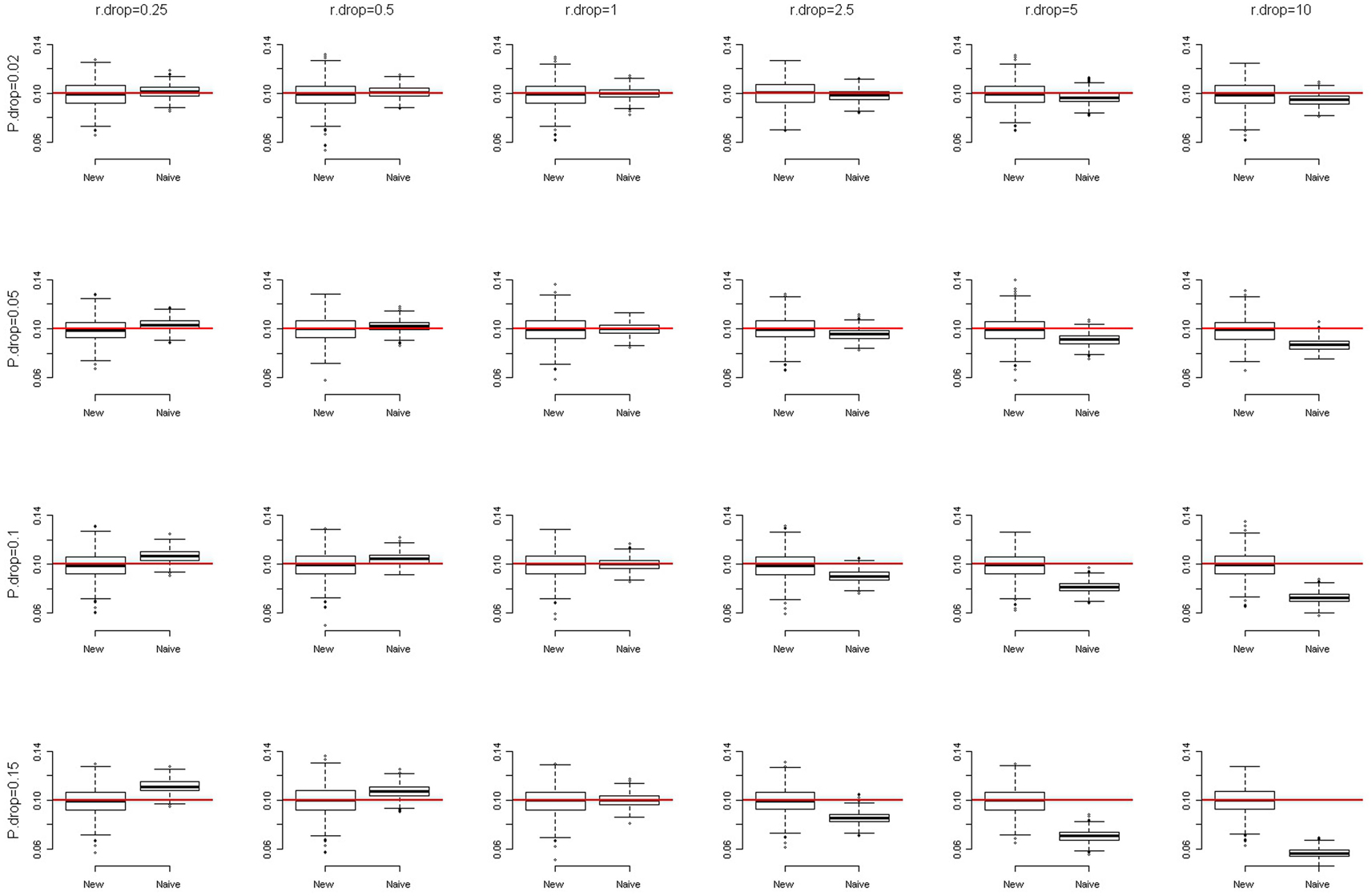
Figure 1. The box-and-whiskers plots of 1,000 estimates of MAF, given MAF = 0.1. The different panels in the figure are arranged so that the overall genotype missing rate (P.drop) is 0.02, 0.05, 0.1, and 0.15 (from top to bottom) and the DDR (r.drop) is 0.25, 0.5, 1, 2.5, 5, and 10 (from left to right). A box is constructed with a median (here, very close to the mean) and two quartiles (the first and the third quartiles). The outliers are data points outside the range of (first quartile −1.5 × IQR, third quartile +1.5 × IQR), where IQR is the inter-quartile range (third quartile − first quartile). The end of the upper whisker is the largest data point below the third quartile +1.5 × IQR, while the end of the lower whisker is the smallest data point beyond the first quartile −1.5 × IQR.

Although our method can improve the accuracy, the precision (inverse variance) of the allele frequency estimates is lowered. Therefore, when DDR = 1, the naïve method is superior to our method, with consideration of both the accuracy and the precision. This is expected because our method involves more parameters (α_Hom, α_Het, and p_A) than does the naïve method (p_A), which lowers the precision of estimates in our method.

Simulation Study: Impact of Hardy–Weinberg Disequilibrium

To evaluate the sensitivity of our method to the assumption of HWE, we performed a simulation study to examine the bias of allele frequency estimates when the assumption of HWE does not hold. The probabilities of the true genotype being AA, AB, and BB can be represented as:

$\begin{array}{llll}& Pr\left(\text{T}=\text{AA}\right)=p_{\text{A}}^2+p_{\text{A}}\left(1-p_{\text{A}}\right)f,& & \\ & Pr\left(\text{T}=\text{AB}\right)=2p_{\text{A}}\left(1-p_{\text{A}}\right)\left(1-f\right),& & \\ & Pr\left(\text{T}=\text{BB}\right)={\left(1-p_{\text{A}}\right)}^2+p_{\text{A}}\left(1-p_{\text{A}}\right)f,& & \end{array}$

where f is the fixation index (Weir, 1996; Wakefield, 2010), a measure of the departure from HWE. When f = 0, there is no departure from HWE. The larger the departure of f from 0, the larger the degree of HWD. When f is positive, the departure from HWE results in excess homozygosity. When f is negative, the departure from HWE results in excess heterozygosity. We simulated a SNP with MAF of 0.1. The total sample size was set at 2,000. Following the setting of fixation index when Chen and Kao (2006) examined the sensitivity of their method to the assumption of HWE, we also evaluated the performance of our method with the fixation index f of 0.1 and 0.2. Figures 2 and 3 present the box-and-whiskers plots of the 1,000 estimates of allele frequencies when the fixation index f = 0.1 and 0.2, respectively. We can see that our method leads to an upward bias to the allele frequency estimates when f > 0, and a downward bias when f < 0 (result not shown). Our method is not very robust to the assumption of HWE. This is a caution when applying this approach.

FIGURE 2

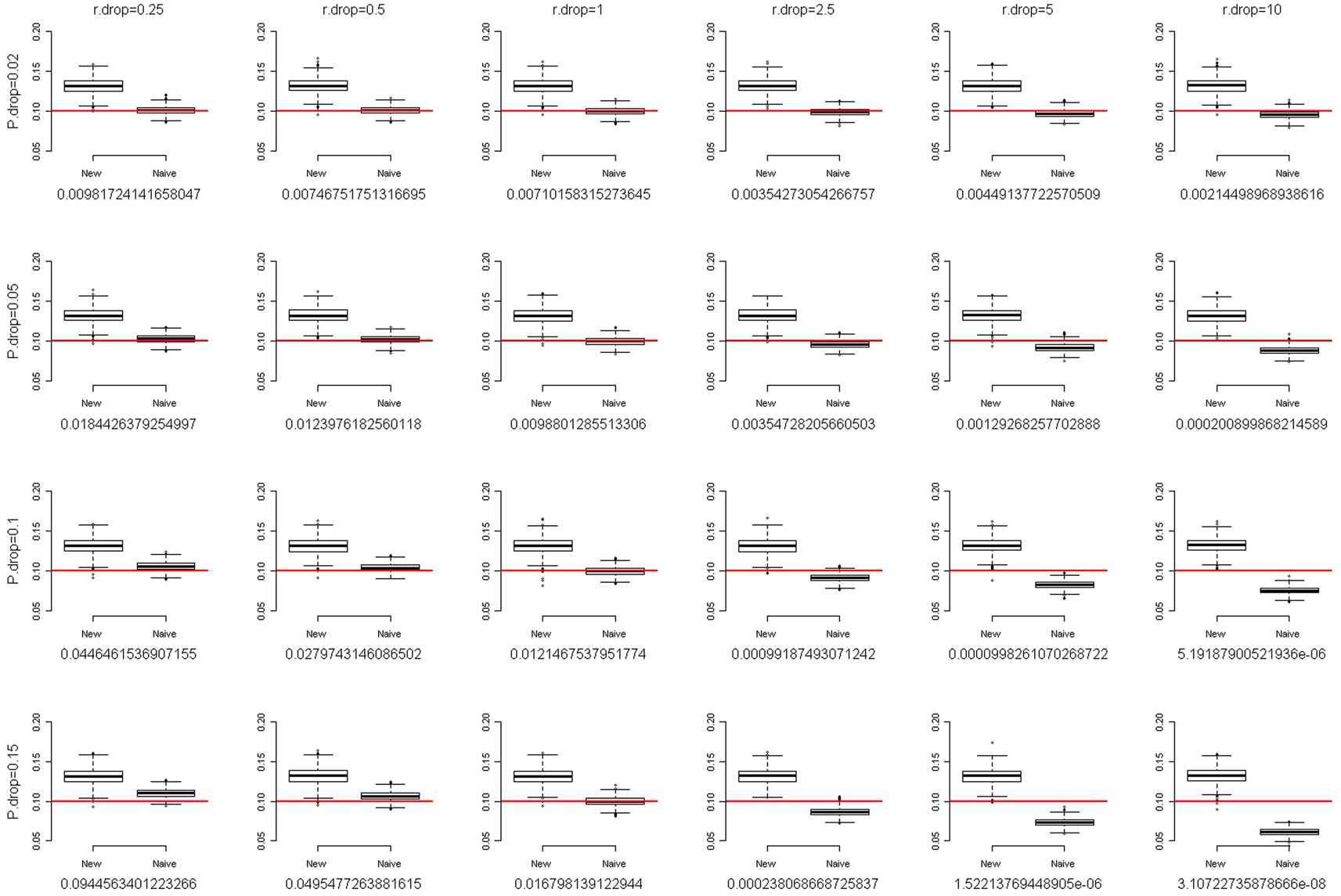
Figure 2. The box-and-whiskers plots of 1,000 estimates of MAF, given MAF = 0.1 and the fixation index f = 0.1. The different panels in the figure are arranged so that the overall genotype missing rate (P.drop) is 0.02, 0.05, 0.1, and 0.15 (from top to bottom) and the DDR (r.drop) is 0.25, 0.5, 1, 2.5, 5, and 10 (from left to right). Below each panel, we list the mean of the 1,000 P values of the exact test for Hardy–Weinberg equilibrium for the 1,000 replications.

FIGURE 3

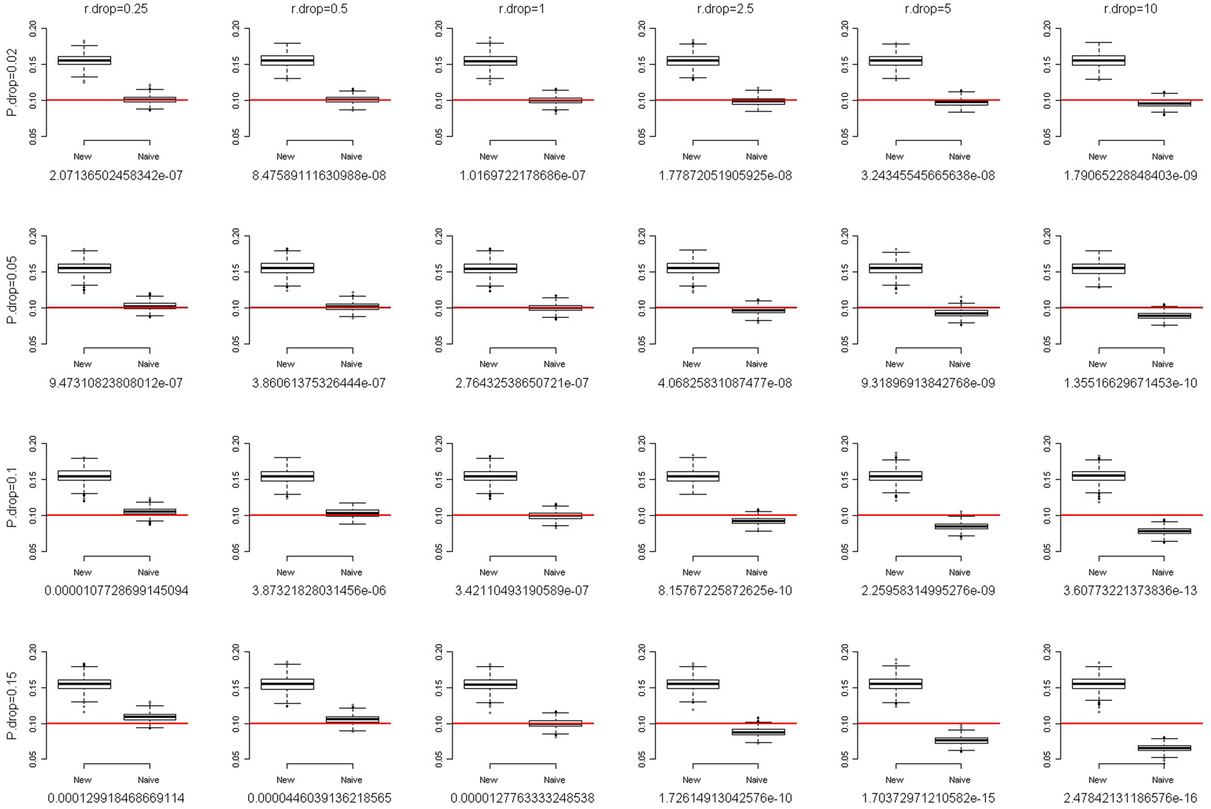
Figure 3. The box-and-whiskers plots of 1,000 estimates of MAF, given MAF = 0.1 and the fixation index f = 0.2. The different panels in the figure are arranged so that the overall genotype missing rate (P.drop) is 0.02, 0.05, 0.1, and 0.15 (from top to bottom) and the DDR (r.drop) is 0.25, 0.5, 1, 2.5, 5, and 10 (from left to right). Below each panel, we list the mean of the 1,000 P values of the exact test for Hardy–Weinberg equilibrium for the 1,000 replications.

For each scenario in Figures 2 and 3, we also provided the mean of the 1,000 P values of the exact test for HWE for the 1,000 replications. Using the observed counts of genotypes AA, AB, and BB, the exact test for HWE (Wigginton et al., 2005) was performed with the R package “Hardy–Weinberg” (Graffelman and Camarena, 2008). When the fixation index f = 0.2 (Figure 3), although our method leads to a large upward bias to the allele frequency estimates, the P values of the exact test for HWE are extremely small (<1.3 × 10⁻⁴). Investigators provided with such significant results for the HWE tests should avoid using our approach. Given the fixation index f = 0.1 (Figure 2), the HWE tests may fail to give researchers an alarm when the overall genotype missing rate (P.drop) is large (0.15) and the DDR is small (0.25). This is because a small DDR (<1) indicates a larger missing rate for homozygotes than for heterozygotes, which dilutes the excess homozygosity linking to a positive fixation index f. If, unfortunately, the overall genotype missing rate (P.drop) is large (here, 0.15), the dilution of excess homozygosity will be even more pronounced. This inconsistency between the observed genotype distribution and the true genotype distribution will induce a blind spot of the HWE test. Nonetheless, overall, performing a HWE test on the observed genotype distribution is a way to evaluate the appropriateness of using our approach.

Application to HapMap Data

We further applied our method to the HapMap data (HapMap, 2005). We downloaded the chromosome 17 genotype data of the 45 Chinese and 44 Japanese released in October, 2005 (HapMap, 2005). We estimated the missing rates of homozygotes (α_Hom) and the missing rates of heterozygotes (α_Het) of these HapMap SNPs, by using our method. After removing SNPs without missing genotypes, we estimated the α_Hom’s and α_Het’s of the remaining SNPs. Figure 4 presents the histograms of the ${\widehat{\alpha }}_{\text{Hom}}^{\prime }$ and ${{\widehat{\alpha }}_{\text{Het}}}^{\prime }$ for the Chinese and Japanese samples, respectively. We can see that the missing rates of heterozygotes are generally larger than the missing rates of homozygotes (DDR > 1), for both the Chinese and Japanese samples. Hao and Cawley (2007) used the Affymetrix genotypes that present no evidence of DDR as benchmark to obtain an estimate of r_drop as 1.73 in the HapMap data. With our method, we estimate r_drop as 1.81 and 1.97 for the Chinese and Japanese samples, respectively.

FIGURE 4

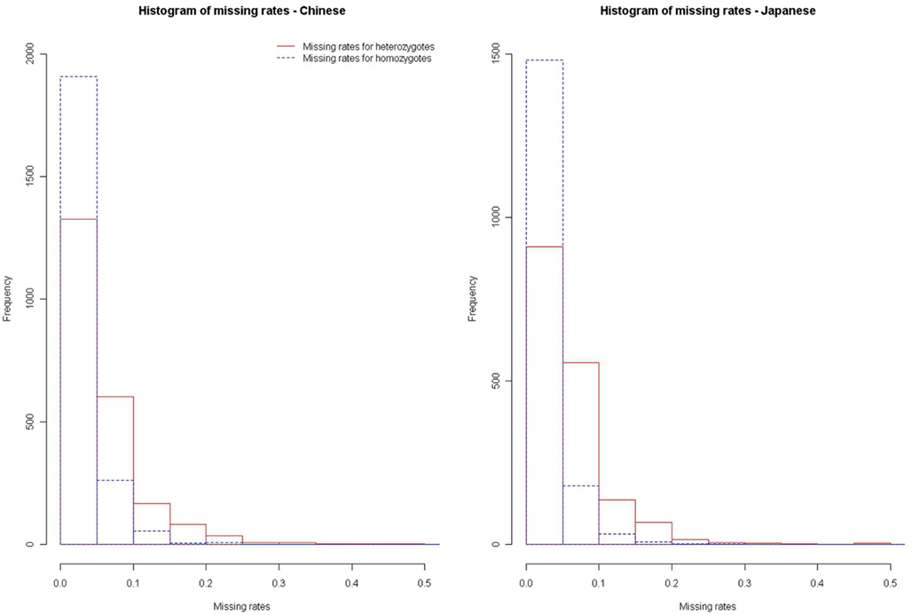
Figure 4. Histograms of missing rates for homozygotes and heterozygotes in the HapMap Chinese and Japanese samples.

Figure 5 shows the interval of point estimate ±standard error of missing rate for each HapMap SNP on chromosome 17. If we approximate the confidence intervals of missing rates with point estimates ±2 × standard errors, all SNPs have overlapped confidence intervals of missing rates for homozygotes and for heterozygotes. For these SNPs, the missing rates for homozygotes and for heterozygotes are not significantly different. This is not unexpected given the small sample sizes of the HapMap data (∼45).

FIGURE 5

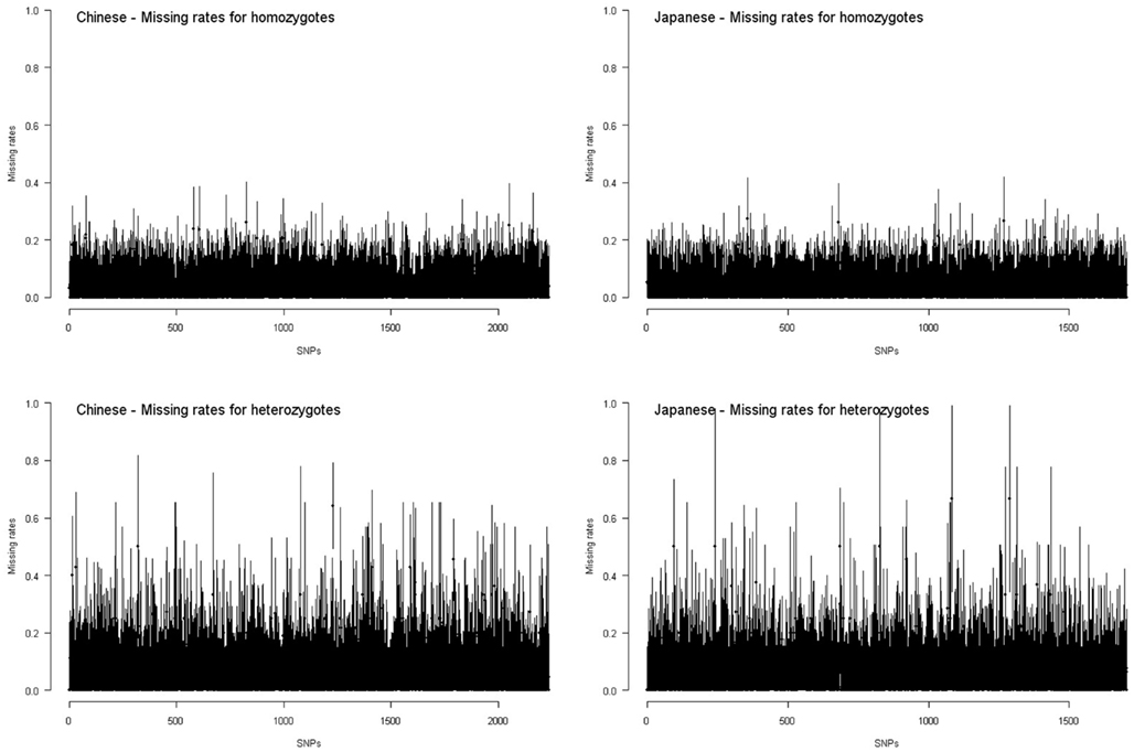
Figure 5. Missing rates for homozygotes and heterozygotes in the HapMap Chinese and Japanese samples. Each interval presents the point estimate ±standard error of missing rate for homozygotes or for heterozygotes of a SNP.

Application to Scleroderma Data

Scleroderma is a chronic autoimmune disease characterized by skin thickening and vascular abnormalities. Scleroderma has an estimated prevalence of 250 patients per million in the United States (Adnan, 2008). There are two main subtypes of scleroderma: diffuse scleroderma and limited scleroderma (Nikpour et al., 2010). The studied data set contains genetic and clinical information collected from the Scleroderma Family Registry and DNA Repository at the University of Texas Health Science Center at Houston (Baugh et al., 2002; Wu et al., 2006). The majority of subjects are white Caucasians. Therefore, we only include the 655 white Caucasians into the analysis. Among the 655 subjects, 160 were diagnosed with diffuse scleroderma, 266 subjects with limited scleroderma, and the remaining 229 subjects were healthy controls. A G/C SNP at position −173 (rs755622) in the 5′ promoter region of migration-inhibitory factor (MIF) was genotyped for each of the 655 subjects. Among the 655 subjects, 15 subjects were missing at SNP rs755622 (MIF − 173 SNP), including 1 (0.63%) patient with diffuse scleroderma, 12 (4.51%) patients with limited scleroderma, and 2 (0.87%) controls. We selected the limited scleroderma patient group (to be the case group) and the control group for the two-sample analysis.

First, we applied the naïve method to the data, by simply removing the subjects with missing genotypes from the analysis. The MAFs in the case and control groups are 12.6 and 18.5%, respectively. The P value of Fisher’s exact test for allelic association is 0.012. Then we applied our method to the data. Based on the observed genotype distribution (AA, ??, AB, and BB), the MAFs in the case and control groups are estimated as 12.1 and 18.4%, respectively. The Fisher’s exact test for allelic association yields a P value of 0.007. Given a significance level of 0.05, both the naïve method and our method suggest an association of the MIF − 173 SNP with scleroderma. Our method gives very similar results with the naïve method. This is expected because the missing rates of genotypes are not high in this example. However, our method provides stronger evidence for the association of the MIF − 173 SNP with scleroderma that was recently confirmed by a study based on a large European population (Bossini-Castillo et al., 2011). The role of the MIF − 173 SNP in scleroderma deserves further investigation.

Discussion

The presence of missing genotypes is common in genetic data. For studies with low-density SNPs, the most commonly used approach for dealing with genotype missingness is to simply remove the observations with missing genotypes from the analyses (Wu et al., 2006). This naïve method is valid only when there is no differential dropout among genotypes. However, in practice, a given assay often has a different capability in typing heterozygotes and homozygotes. Differential dropout among genotypes (a type of informative missingness) is detectable even in data from some carefully designed studies such as the HapMap (HapMap, 2005; Hao and Cawley, 2007) and the WTCCC projects (Wellcome Trust Case Control Consortium, 2007). Although the issue of informatively missing genotypes has been investigated in case-parent study design (Allen et al., 2003; Chen, 2004) and in haplotype data analyses (Liu et al., 2006, 2009a), there is no investigation of this issue on one locus for samples of unrelated individuals.

In this work, we propose a statistical method to estimate allele frequencies and missing rates of heterozygotes and homozygotes, under the assumption of HWE. We perform simulations to compare our method with the naïve method in the estimation of allele frequencies. Under HWE, our method gives accurate estimates for MAFs, with or without differential dropout among genotypes. The naïve method generates accurate estimates for MAFs only when there is no differential dropout among genotypes. We further apply our method to the HapMap data, and obtain similar estimates of DDRs to that estimated by Hao and Cawley (2007) with extra data. In addition, we analyze a scleroderma data set (Baugh et al., 2002; Wu et al., 2006) to show the practical use of our method. In contrast to Hao and Cawley (2007), we do not need to genotype the sample with another gene chip and assume it as the ground truth in order to estimate the DDR. To the best of our knowledge, our method is the only statistical method to handle differential dropout among genotypes on one locus for samples of unrelated individuals.

Despite these merits, there are some limitations in our method. First, although the estimates of MAFs are unbiased under HWE, the precision of the estimates is lowered because our method involves more parameters in the estimation process. Therefore, when there is no differential dropout among genotypes (DDR = 1), the naïve method may perform better than our method, considering both the accuracy and precision of the estimates. Second, our method relies on the assumption of HWE in the true genotype distribution. Although the true genotype distribution is unknown, one way to evaluate the appropriateness of using our approach is to perform a HWE test on the observed genotype distribution.

In this work, we focus on the estimation of allele frequencies, which is an important issue in epidemiological studies (Taioli et al., 2004). A future direction would be to evaluate the performance of our method and the naïve method on association testing.

Conflict of Interest Statement

The authors declare that the research was conducted in the absence of any commercial or financial relationships that could be construed as a potential conflict of interest.

Acknowledgments

We thank the reviewers for their insightful and constructive comments; Dr. Richard Bucala for kindly providing the scleroderma data. This work was supported in part by NIH grant GM081488 (NL) from the National Institutes of Health. The content is solely the responsibility of the authors and does not necessarily represent the official views of the National Institutes of Health. The authors declare that they have no conflict of interest.

References

Adnan, Z. A. (2008). Diagnosis and treatment of scleroderma. Acta Med. Indones. 40, 109–112.

Pubmed Abstract | Pubmed Full Text

Allen, A. S., Rathouz, P. J., and Satten, G. A. (2003). Informative missingness in genetic association studies: case-parent designs. Am. J. Hum. Genet. 72, 671–680.

Pubmed Abstract | Pubmed Full Text | CrossRef Full Text

Baugh, J. A., Chitnis, S., Donnelly, S. C., Monteiro, J., Lin, X., Plant, B. J., Wolfe, F., Gregersen, P. K., and Bucala, R. (2002). A functional promoter polymorphism in the macrophage migration inhibitory factor (MIF) gene associated with disease severity in rheumatoid arthritis. Genes Immun. 3, 170–176.

Pubmed Abstract | Pubmed Full Text | CrossRef Full Text

Bossini-Castillo, L., Simeon, C. P., Beretta, L., Vonk, M. C., Callejas-Rubio, J. L., Espinosa, G., Carreira, P., Camps, M. T., Rodriguez-Rodriguez, L., Rodriguez-Carballeira, M., Garcia-Hernandez, F. J., Lopez-Longo, F. J., Hernandez-Hernandez, V., Saez-Comet, L., Egurbide, M. V., Hesselstrand, R., Nordin, A., Hoffmann-Vold, A. M., Vanthuyne, M., Smith, V., De Langhe, E., Kreuter, A., Riemekasten, G., Witte, T., Hunzelmann, N., Voskuyl, A. E., Schuerwegh, A. J., Lunardi, C., Airo, P., Scorza, R., Shiels, P., van Laar, J. M., Fonseca, C., Denton, C., Herrick, A., Worthington, J., Koeleman, B. P., Rueda, B., Radstake, T. R., and Martin, J. (2011). Confirmation of association of the macrophage migration inhibitory factor gene with systemic sclerosis in a large European population. Rheumatology (Oxford) 50, 1976–1981.

Pubmed Abstract | Pubmed Full Text

Calus, M. P., Veerkamp, R. F., and Mulder, H. A. (2011). Imputation of missing single nucleotide polymorphism genotypes using a multivariate mixed model framework. J. Anim. Sci. 89, 2042–2049.

Pubmed Abstract | Pubmed Full Text | CrossRef Full Text

Chen, Y. H. (2004). New approach to association testing in case-parent designs under informative parental missingness. Genet. Epidemiol. 27, 131–140.

Pubmed Abstract | Pubmed Full Text | CrossRef Full Text

Chen, Y. H., and Kao, J. T. (2006). Multinomial logistic regression approach to haplotype association analysis in population-based case-control studies. BMC Genet. 7, 43.

CrossRef Full Text

Daetwyler, H. D., Wiggans, G. R., Hayes, B. J., Woolliams, J. A., and Goddard, M. E. (2011). Imputation of missing genotypes from sparse to high density using long-range phasing. Genetics 189, 317–327.

Pubmed Abstract | Pubmed Full Text | CrossRef Full Text

Dempster, A. P., Laird, N. M., and Rubin, D. B. (1977). Maximum likelihood estimation from incomplete data via the EM algorithm. J. R. Stat. Soc. Series B Methodol. 39, 1–38.

Druet, T., Schrooten, C., and De Roos, A. P. (2010). Imputation of genotypes from different single nucleotide polymorphism panels in dairy cattle. J. Dairy Sci. 93, 5443–5454.

Pubmed Abstract | Pubmed Full Text | CrossRef Full Text

Epstein, M. P., and Satten, G. A. (2003). Inference on haplotype effects in case-control studies using unphased genotype data. Am. J. Hum. Genet. 73, 1316–1329.

Pubmed Abstract | Pubmed Full Text | CrossRef Full Text

Excoffier, L., and Slatkin, M. (1995). Maximum-likelihood estimation of molecular haplotype frequencies in a diploid population. Mol. Biol. Evol. 12, 921–927.

Pubmed Abstract | Pubmed Full Text

Graffelman, J., and Camarena, J. M. (2008). Graphical tests for Hardy-Weinberg equilibrium based on the ternary plot. Hum. Hered. 65, 77–84.

Pubmed Abstract | Pubmed Full Text | CrossRef Full Text

Greenland, S., and Finkle, W. D. (1995). A critical look at methods for handling missing covariates in epidemiologic regression analyses. Am. J. Epidemiol. 142, 1255–1264.

Pubmed Abstract | Pubmed Full Text

Hao, K., and Cawley, S. (2007). Differential dropout among SNP genotypes and impacts on association tests. Hum. Hered. 63, 219–228.

Pubmed Abstract | Pubmed Full Text | CrossRef Full Text

HapMap. (2005). A haplotype map of the human genome. Nature 437, 1299–1320.

Pubmed Abstract | Pubmed Full Text | CrossRef Full Text

Kang, H., Qin, Z. S., Niu, T., and Liu, J. S. (2004). Incorporating genotyping uncertainty in haplotype inference for single-nucleotide polymorphisms. Am. J. Hum. Genet. 74, 495–510.

Pubmed Abstract | Pubmed Full Text | CrossRef Full Text

Liu, N., Beerman, I., Lifton, R., and Zhao, H. (2006). Haplotype analysis in the presence of informatively missing genotype data. Genet. Epidemiol. 30, 290–300.

Pubmed Abstract | Pubmed Full Text | CrossRef Full Text

Liu, N., Bucala, R., and Zhao, H. (2009a). Modeling informatively missing genotypes in haplotype analysis. Commun. Stat Theory Methods 38, 3445–3460.

CrossRef Full Text

Liu, N., Zhang, D., and Zhao, H. (2009b). Genotyping error detection in samples of unrelated individuals without replicate genotyping. Hum. Hered. 67, 154–162.

CrossRef Full Text

Marchini, J., Howie, B., Myers, S., Mcvean, G., and Donnelly, P. (2007). A new multipoint method for genome-wide association studies by imputation of genotypes. Nat. Genet. 39, 906–913.

Pubmed Abstract | Pubmed Full Text | CrossRef Full Text

Matsuzaki, H., Dong, S., Loi, H., Di, X., Liu, G., Hubbell, E., Law, J., Berntsen, T., Chadha, M., Hui, H., Yang, G., Kennedy, G. C., Webster, T. A., Cawley, S., Walsh, P. S., Jones, K. W., Fodor, S. P., and Mei, R. (2004). Genotyping over 100,000 SNPs on a pair of oligonucleotide arrays. Nat. Methods 1, 109–111.

Pubmed Abstract | Pubmed Full Text | CrossRef Full Text

Nikpour, M., Stevens, W. M., Herrick, A. L., and Proudman, S. M. (2010). Epidemiology of systemic sclerosis. Best Pract. Res. Clin. Rheumatol. 24, 857–869.

Pubmed Abstract | Pubmed Full Text | CrossRef Full Text

Oliphant, A., Barker, D. L., Stuelpnagel, J. R., and Chee, M. S. (2002). BeadArray technology: enabling an accurate, cost-effective approach to high-throughput genotyping. Biotechniques 56, 60–61.

Rubin, D. B. (1976). Inference and missing data. Biometrika 63, 581–592.

CrossRef Full Text

Stephens, M., and Scheet, P. (2005). Accounting for decay of linkage disequilibrium in haplotype inference and missing-data imputation. Am. J. Hum. Genet. 76, 449–462.

Pubmed Abstract | Pubmed Full Text | CrossRef Full Text

Taioli, E., Pedotti, P., and Garte, S. (2004). Importance of allele frequency estimates in epidemiological studies. Mutat. Res. 567, 63–70.

Pubmed Abstract | Pubmed Full Text | CrossRef Full Text

Wakefield, J. (2010). Bayesian methods for examining Hardy-Weinberg equilibrium. Biometrics 66, 257–265.

Pubmed Abstract | Pubmed Full Text | CrossRef Full Text

Weir, B. (1996). Genetic Data Analysis II. Sunderland, MA: Sinauer.

Wellcome Trust Case Control Consortium. (2007). Genome-wide association study of 14,000 cases of seven common diseases and 3,000 shared controls. Nature 447, 661–678.

Pubmed Abstract | Pubmed Full Text | CrossRef Full Text

Wigginton, J. E., Cutler, D. J., and Abecasis, G. R. (2005). A note on exact tests of Hardy-Weinberg equilibrium. Am. J. Hum. Genet. 76, 887–893.

Pubmed Abstract | Pubmed Full Text | CrossRef Full Text

Wu, S. P., Leng, L., Feng, Z., Liu, N., Zhao, H., Mcdonald, C., Lee, A., Arnett, F. C., Gregersen, P. K., Mayes, M. D., and Bucala, R. (2006). Macrophage migration inhibitory factor promoter polymorphisms and the clinical expression of scleroderma. Arthritis Rheum. 54, 3661–3669.

Pubmed Abstract | Pubmed Full Text | CrossRef Full Text

Yu, Z., and Schaid, D. J. (2007). Methods to impute missing genotypes for population data. Hum. Genet. 122, 495–504.

Pubmed Abstract | Pubmed Full Text | CrossRef Full Text

Zhang, B., Zhi, D., Zhang, K., Gao, G., Limdi, N. A., and Liu, N. (2011). Practical consideration of genotype imputation: sample size, window size, reference choice, and untyped rate. Stat. Interface 4, 339–352.

Pubmed Abstract | Pubmed Full Text | CrossRef Full Text

Zhao, Z., Timofeev, N., Hartley, S. W., Chui, D. H., Fucharoen, S., Perls, T. T., Steinberg, M. H., Baldwin, C. T., and Sebastiani, P. (2008). Imputation of missing genotypes: an empirical evaluation of IMPUTE. BMC Genet. 9, 85.

Pubmed Abstract | Pubmed Full Text | CrossRef Full Text

Appendix

The identifiability of the three model parameters (α_Hom, α_Het, and p_A)

For the model shown in Table 1, we assume that none of p₁, p₂, p₃, and p₄ are zero. We have

$\begin{array}{llll}{p}_1& =Pr\left(\text{O}=\text{AA}\right)=\left(1-{\alpha }_{\text{Hom}}\right)\cdot p_A^2& & \text{(A1)}\\ p_2& =Pr\left(\text{O}=??\right)={\alpha }_{\text{Hom}}{p}_A^2+{\alpha }_{\text{Hom}}{\left(1-p_{\text{A}}\right)}^2& & \\ & +{\alpha }_{\text{Het}}2p_{\text{A}}\left(1-p_{\text{A}}\right)& & \text{(A2)}\\ p_3& =Pr\left(\text{O}=\text{AB}\right)=\left(1-{\alpha }_{\text{Het}}\right)2p_{\text{A}}\left(1-p_{\text{A}}\right)& & \text{(A3)}\\ p_4& =Pr\left(\text{O}=\text{BB}\right)=\left(1-{\alpha }_{\text{Hom}}\right){\left(1-p_{\text{A}}\right)}^2& & \text{(A4)}\end{array}$

Define $C=\sqrt{\frac{p_1}{p_4}}=\frac{p_{\text{A}}}{\left(1-p_{\text{A}}\right)}.$ Then we have $p_{\text{A}}=\frac{C}{1+C}=\frac{\sqrt{p_1}}{\sqrt{p_1}+\sqrt{p_4}}.$

From (A3), we have

$\begin{array}{llll}{\alpha }_{\text{Het}}& =1-\frac{p_3}{2p_{\text{A}}\left(1-p_{\text{A}}\right)}=1-\frac{p_3}{2\left(\frac{C}{1+C}\right)\left(\frac{1}{1+C}\right)}& & \\ & =1-\frac{p_3{\left(\sqrt{p_1}+\sqrt{p_4}\right)}^2}{2\sqrt{p_1{p}_4}}.& & \end{array}$

Similarly, from (A1), we have

$\begin{array}{llll}{\alpha }_{\text{Hom}}& =1-\frac{p_1}{p_{\text{A}}^2}=1-\frac{p_1}{\frac{C^2}{{\left(1+C\right)}^2}}=1-\frac{p_1{\left(1+C\right)}^2}{C^2}& & \\ & =1-p_4{\left(1+C\right)}^2=1-{\left(\sqrt{p_1}+\sqrt{p_4}\right)}^2.& & \end{array}$

The three parameters (α_Hom, α_Het, and p_A) are thus all identifiable.