Abstract
Achieving feasible, smooth and efficient trajectories for autonomous vehicles which appropriately take into account the long-term future while planning, has been a long-standing challenge. Several approaches have been considered, roughly falling under two categories: rule-based and learning-based approaches. The rule-based approaches, while guaranteeing safety and feasibility, fall short when it comes to long-term planning and generalization. The learning-based approaches are able to account for long-term planning and generalization to unseen situations, but may fail to achieve smoothness, safety and the feasibility which rule-based approaches ensure. Hence, combining the two approaches is an evident step towards yielding the best compromise out of both. We propose a Reinforcement Learning-based approach, which learns target trajectory parameters for fully autonomous driving on highways. The trained agent outputs continuous trajectory parameters based on which a feasible polynomial-based trajectory is generated and executed. We compare the performance of our agent against four other highway driving agents. The experiments are conducted in the Sumo simulator, taking into consideration various realistic, dynamically changing highway scenarios, including surrounding vehicles with different driver behaviors. We demonstrate that our offline trained agent, with randomly collected data, learns to drive smoothly, achieving velocities as close as possible to the desired velocity, while outperforming the other agents.
1 Introduction
In the recent past, autonomous driving (AD) on highways has been a very active area of research (Katrakazas et al., 2015; Schwarting et al., 2018). The autonomous vehicle should be able to respect traffic rules, yield, merge, change lanes, overtake, anticipate cut-ins in a comfortable and safe but not overly conservative manner. Numerous approaches have been proposed that can be broadly divided into two categories: approaches that do not learn from data such as rule-based or optimal-control based approaches (Claussmann et al., 2019), and machine learning-based (ML) approaches (Grigorescu et al., 2020). The former rely either on a set of rules tuned by human experience, or are formulated as an optimization problem subject to various constraints, aiming for a solution with the lowest cost (Borrelli et al., 2005; Falcone et al., 2007; Glaser et al., 2010; Werling et al., 2010; Xu et al., 2012). Usually they are based on mathematically sound safety rules and are able to provide feasible and smooth driving trajectories (Rao, 2010). However, it is difficult to anticipate all possible behaviors of other vehicles and objects on the highway and translate them into all-encompassing rules. Doing so could lead to errors in the rules and false assumptions about the behavior of other drivers. Similarly, optimization-based approaches can get computationally demanding in complex, highly dynamic traffic settings due to the real-time constraint of the solver. Additionally, the limited planning horizon in optimization based approaches results in difficulties when planning long-term, which may lead to a sub-optimal overall performance. Alternatively, machine learning-based approaches, learn from data and are able to generalize to the aforementioned uncertain situations, making the system more robust and less prone to errors caused by false assumptions (Kuutti et al., 2021). Since acquiring high-quality labeled data is cumbersome and expensive, Reinforcement Learning (RL) in particular offers a good alternative for tackling the autonomous driving problem (Hoel et al., 2018; Mirchevska et al., 2018; Wang et al., 2019; Hügle et al., 2019; Nageshrao et al., 2019; Huegle et al., 2020; Kalweit et al., 2020; 2021; Mirchevska et al., 2021). Based on the type of the actions the agent learns to perform, we can categorize RL-based approaches into high-level, low-level, and approaches that combine both. High-level action approaches are the ones where the agent may choose from a few discrete actions defining some high-level maneuver like keep lane or perform a lane-change (Mirchevska et al., 2017; Mukadam et al., 2017; Mirchevska et al., 2018; Wang et al., 2019; Hügle et al., 2019). They are limiting in a sense that the maneuvers behind the lane-change actions usually are fixed and not well adjusted to every situation that might occur. For example, the lane-change maneuver always has the same duration regardless of the situation and the agent is unable to choose exactly where to end up after a lane-change (behind or in front of an adjacent vehicle, etc.). In low-level approaches such as (Wang et al., 2019; 2018; Wang et al., 2019; Kaushik et al., 2018; Kendall et al., 2018; Saxena et al., 2019) the agent usually outputs actions that directly influence the lowest level of control such as acceleration and steering wheel. Since the low-level approaches do not rely on any underlying structure, everything needs to be learned from scratch, requiring large amounts of high-quality data and very long training times. At the same time, high-level approaches may make it too difficult to obtain smooth and feasible trajectories that are customized for each given situation. This is because lower level maneuvers are usually hard-coded and fixed in terms of duration and shape.
To get the best of both worlds, fast learning and long-term planning for RL and mathematical stability for the model-based methods, the combination of the two holds the promise to speed up and improve the learning process. It enables a trade-off between high- and low-level actions by allowing flexibility for the RL agent, to have increased control over the final decision, while avoiding the need to learn tasks that are efficiently handled by traditional control methods. Most methods combining trajectory optimization with RL separate the RL agent from the trajectory decision (Bellegarda and Byl, 2019; Ota et al., 2019; Bogdanovic et al., 2021; Mirchevska et al., 2021) or discretize the action space (Hoel et al., 2019; Nageshrao et al., 2019; Ronecker and Zhu, 2019). This may result in sub-optimal behavior since the RL agent has limited awareness of the criteria used to generate the final trajectory. In (Mirchevska et al., 2021) we developed an RL agent that first chooses the best candidate from a set of gaps (space between two surrounding vehicles on the same lane) to fit into (in order to change a lane or stay in the current lane), and then triggers a trajectory planner to choose the best trajectory to get there. Even though the agent performed well, this procedure is costly since it entails defining all gaps and the trajectories reaching them at run-time, including checks for collisions and assessing velocities before proposing the available actions to the agent.
To address this, here we are proposing a continuous control trajectory optimization approach based on RL. Every second, the agent chooses four continuous actions describing the target trajectory parameters as shown in Figure 1. This provides the flexibility to directly choose the parameters for the generation of the trajectory that it is going to be executed until the next time-step. Furthermore, instead of learning how to generate the trajectories, we delegate this task to a well-established polynomial-based trajectory generation module.
FIGURE 1
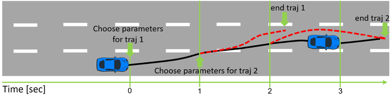
Our approach combines Reinforcement Learning and a polynomial-based trajectory planner to generate updated trajectories every second. The RL algorithm sets the desired target values for parameters of the trajectories including lateral position, lateral profile duration, longitudinal velocity and longitudinal profile duration.
In many applications, the need for learning a good policy using only a pre-collected set of data
1, becomes evident since learning while interacting with the environment is either too expensive or dangerous. Autonomous driving is considered to be one of them, where in production application, the data is usually first collected and then used offline (
Levine et al., 2020). Considering that, we conduct the training using only data collected with a simple random policy in an offline fashion. The trained agent is evaluated on realistic
2, highly dynamic highway scenarios that simulate human-like driving behaviors, using parameters that encompass a range of driving styles including variations in reaction times, cooperativeness and aggressiveness, among others. These scenarios involve a varying number of traffic participants that are randomly positioned on the road to ensure a comprehensive assessment of the agent’s performance, taking into account the fact that the surrounding vehicles have also varying driving goals in terms of target driving speed. We show that the agent learns to drive smoothly and as close as possible to the desired velocity, while outperforming the comparison agents. It is also able to handle unpredictable situations such as sudden cut-ins and scenarios where more complex maneuvers are required. Additionally, we perform quantitative analysis to show how the nature of the training data and the percentage of terminal samples included influence the learned policy. Our main contributions are the following.
1. A novel offline RL-based approach for AD on highways with continuous control for separate lateral and longitudinal planning components resting on an underlying polynomial-based trajectory generation module.
2. Comparison against other models, on diverse realistic highway scenarios with surrounding vehicles controlled by different driver types.
3. Demonstrating that the agent has learned to successfully deal with critical situations such as sudden cut-ins and scenarios where more complex maneuvers are required.
4. Analysis of the training data by considering the structure of the data and the proportion of terminal samples3.
2 Reinforcement learning background
In RL an agent learns to perform specific tasks from interactions with the environment. RL problems are usually modeled as a Markov Decision Process (MDP) , where is the set of states, the set of actions and is the transition model. At each time-step t, the agent finds itself in a state st and acts by executing an action at, in the environment. As a consequence of taking action at, the agent transitions to the next state st+1 and receives a feedback value rt+1 from the environment, called a reward. The feedback is a measure of success or failure of the agent’s actions. The agent’s objective is to find a policy π, i.e., a mapping from states to actions that maximizes the expected discounted sum of rewards accumulated over time, defined as . The discount factor γ ∈ [0, 1] regulates the importance of future rewards. The performance of the agent, following the policy π, can be measured using the action-value function . The agent infers the optimal policy at a state st from the optimal state-action value function Q*(st, at) = maxπQπ(st, at), via maximization. Another way to learn the parameterized policy is directly by using policy gradient methods.
The common way of dealing with RL problems with continuous actions, as the problem discussed in this paper, are the Actor-Critic methods, which are integrating both value iteration and policy gradient. The actor represents the policy and is used to select actions, whereas the critic represents the estimated value function and evaluates the actions taken by the actor.
In offline RL, instead of learning while interacting with the environment, the agent is provided with a fixed batch of transition samples, i.e., interactions with the environment, to learn from. This data has been previously collected by one or a few policies unknown to the agent. Offline RL is considered more challenging than online RL because the agent does not get to explore the environment based on the current policy, but it is expected to learn only from pre-collected data. For more details and background on RL refer to Sutton and Barto (2018).
3 Approach
The trajectory parameters learning framework consists of four modules: scene understanding, planning/decision making, trajectory generation and trajectory execution, illustrated in Figure 2. Their interconnections are explained in the following.
FIGURE 2
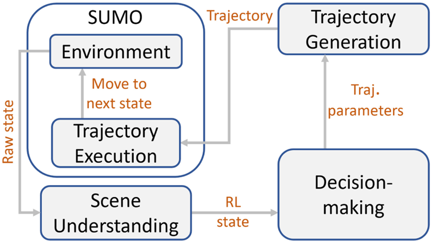
From the Sumo simulator, the complete raw environment state (including information for the RL agent and its surroundings) is sent to the scene understanding module. There, specific features are selected, defining the RL state used for learning which is sent to the decision-making module. Once a decision is made in the form of trajectory parameters, they are then propagated to the trajectory generation module. The trajectory generation module generates the trajectory based on the input parameters and forwards it to the trajectory execution module. Finally, the trajectory execution module, sends the corresponding signals to Sumo to move the RL agent to the next state.
3.1 Scene understanding
The scene understanding module is in charge of collecting information from the environment and processing it into RL state features relevant for decision making. It consists of information about the RL agent, the surrounding vehicles and the road infrastructure. For this purpose we use the DeepSets implementation adapted from Hügle et al. (2019), which is allowing for variable number of inputs from the environment. This is helpful because it alleviates the need to pre-define which and how many objects from the environment are relevant for the decision making.
3.2 Decision making
The decision-making module is implemented based on the Twin Delayed Deep Deterministic policy gradient (TD3) algorithm (Fujimoto et al., 2018). TD3 is an actor-critic, off-policy algorithm that is suitable for environments with continuous action spaces. We randomly initialize an actor (policy) network πθ and three critic networks4. Given a fixed batch of training samples , each training iteration we select a mini-batch of samples from . In each sample (s, a, r′, s′, done), s represents the output of the DeepSets, describing the environment in terms of the surrounding vehicles, concatenated with the state-features describing the RL agent. The complete training algorithm, Offline Trajectory Parameters Learning (OTPL) is described in Algorithm 1.
Algorithm 1
Input: Random initial parameters θ for actor policy πθ,
wi for critics ,
Fixed replay buffer , mini-batch size,
Target parameters: θ′ ←θ; ,
Noise clipping value c, policy delay value d,
Target policy noise: ,
for training iteration h = 1, 2, … do
get mini-batch from
for each ransition sample (s, a, r′, s′, done) in do
Compute target actions:
Compute target:
Update critics by 1 step of gradient descent:
ifh mod d = = 0 then
Update actor by the det. policy gradient:
Update targets:
θ′ ← τθ + (1 − τ)θ′
end if
end for
end for
Once the training is done and we have a well-performing trained agent, we apply it on unseen scenarios for evaluation. Based on the current RL state s = (ρ, srl), which is a concatenation of the DeepSets processed state of the surrounding vehicles, ρ and the RL agent state srl, the RL agent selects a new action, consisting of four continuous sub-actions representing the target trajectory parameters described in Section 4.2. Based on the selected trajectory parameters, a trajectory is generated and checked for safety. If the trajectory is safe, the first 1 s of it is executed, after which the RL agent selects a new action. If it is unsafe, the scenario ends unsuccessfully. The action execution algorithm for a trained agent is described in Algorithm 2.
Algorithm 2. Trained OTPL agent action selection
-
Input: Combined state s = (ρ, srl), where
-
ρ is the DeepSets output environment state,
-
srl is RL agent state,
-
Trained agent πθ
-
while evaluation scenario not finished do
-
compute RL action components:
-
-
generate trajectory t:
-
-
ift is safe then
-
Execute first second of t
-
else
-
fail = True; break
-
end if
-
end while
-
if not failthen return success
-
end if
3.3 Trajectory generation
After the RL agent has made a decision, the chosen continuous actions are forwarded to the trajectory generation module. The actions are values for the parameters that describe the desired trajectory. Based on the current environment state and on the parameters coming from the RL agent’s action, a polynomial trajectory is generated consisting of longitudinal and lateral movement components. The longitudinal movement is described using a quartic (fourth order) polynomial, while for generating the lateral movement, quintic (fifth order) polynomials are considered more suitable. We describe in detail how the trajectory generation works in the Appendix. For additional information the reader can also refer to Werling et al. (2010). Since the RL agent makes a new decision every second, we set the target longitudinal acceleration, target lateral acceleration and the target lateral velocity for each chosen trajectory to zero5, without loss of feasibility or smoothness. This is because the reward function punishing high longitudinal and lateral jerk values makes sure the agent avoids choosing trajectories with short duration and high changes in velocity. We are setting the target longitudinal and lateral acceleration, and the target lateral velocity to zero so that we can solve the Appendix Eqs. 3, 4. needed for generating the trajectory. Given the 4 actions chosen by the agent specified in Section 4.2, by solving the equations we retrieve the values for target longitudinal and lateral positions, target velocity and target orientation to be sent and executed by the RL agent. In Figure 3 we illustrate an example of a trajectory selection over the course of approximately 8 s, in terms of the lateral velocity.
FIGURE 3
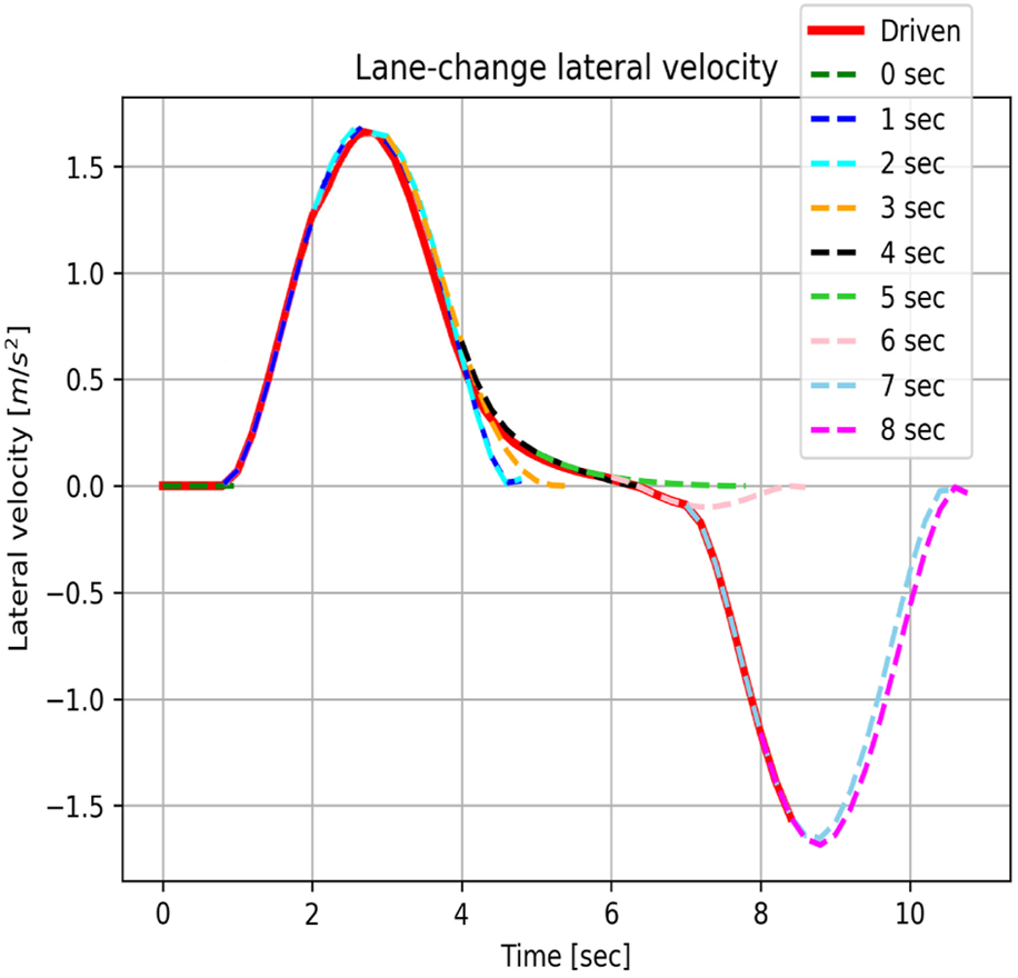
Example trajectory selection during a lane‐change. The trajectories chosen each second are indicated with different colors. The complete driven trajectory is shown in red.
3.4 Trajectory execution
After the target trajectory has been generated and checked for safety, it is sent for execution. Each time-step (0.2 s), values from the trajectory for target longitudinal and lateral positions, target velocity and target orientation are sent and executed. Once five time-steps are done, i.e., after one second, the agent finds itself in the next RL state, where it makes a new decision. The RL agent re-calculates the decision every second because one second corresponds to the standard driving reaction time (Hugemann, 2002). In order for the vehicle to move smoothly, the trajectory contains values for every 0.2 s, which also corresponds to the time-step size of the Sumo simulator.
4 MDP formalization
We consider the problem of safe and smooth driving in realistic highway scenarios, among other traffic participants with varying driving styles. Additionally, the agent needs to maintain its velocity as close as possible to a desired one. In this section we describe the RL components and the data used for training.
4.1 RL state
The RL state consists of two components, one describing the RL agent and the other referring to the surrounding vehicles in a certain radius around the RL agent. The RL agent is described by the features specified in Table 1, whereas the ones describing the surrounding vehicles of the RL agent are specified in Table 2.
TABLE 1
| Feature | Definition |
|---|---|
| Longitudinal velocity | |
| Left lane valid flag | llv ∈ {0, 1} |
| Right lane valid flag | rlv ∈ {0, 1} |
| Lateral position | |
| Longitudinal acceleration | |
| Lateral velocity | |
| Lateral acceleration |
State features describing the RL agent.
TABLE 2
| Feature | Definition |
|---|---|
| Relative distance | rd k = plon,k − plon, where plon and plon,k are the longitudinal positions |
| of the RL agent and the considered vehicle k respectively | |
| Relative longitudinal velocity | rv lon,k = (vlon,k − vlon)/vdes, where vlon,k is the absolute lon |
| velocity of the vehicle k and vdes is the user-defined desired lon. velocity | |
| Relative lane | rl k = lk − l, where l and lk are the lane ids of the RL agent |
| and the kth surrounding vehicle respectively |
State features describing the surrounding vehicles of the RL agent.
4.2 Actions
The agent learns to perform an action a, consisting of four continuous sub-actions, detailed in Table 3. These four actions represent the minimal set of parameters needed for generating a trajectory, in compliance with the trajectory generation procedure explained in Figure 3.
TABLE 3
| Sub-action | Definition |
|---|---|
| Target trajectory longitudinal velocity | |
| Target trajectory longitudinal profile duration | |
| Target trajectory lateral profile duration | |
| Target lateral position |
Action space definition.
4.3 Reward
The reward function is designed to take into consideration three driving objectives. First, the RL agent should not cause collisions and remain within the road boundaries, second, it should drive as close as possible to a pre-defined desired velocity, and third, the RL agent should be encouraged to drive in a smooth manner. Before we assemble the final reward function, we will define the components needed to describe each of the three objectives. For the first objective, not causing collisions and remaining within the road boundaries, we define an indicator f signaling when the agent has failed in the following way:For the second objective, driving as close as possible to the desired velocity vdes, we define:and an indicator indv signaling whether the agent drives below the desired velocity:
Where vlon is the current longitudinal velocity of the RL agent. For the third objective, driving smoothly, we need to control the longitudinal and lateral jerk values6. Regarding the longitudinal jerk, we define:which represents the averaged sum of all squared longitudinal jerk values jlon in the trajectory generated from action a, where n is the number of time-steps in the trajectory. pjlon is a jerk penalty value, is the maximum averaged sum of squared jerk value encountered in the training data and indj is an indicator denoted by:Analogously, we define the same for the lateral jerk:as well as indjlat, pjlat and .
All three objectives are combined in the final reward function as shown in Eq. 7.We provide details regarding the action boundaries and the choice of the jerk penalties in the code repository.
5 Data collection and implementation
5.1 Training data
We collected around 5 × 10⁵ data-samples varying the initial position and the behavior of the surrounding vehicles in dynamic highway scenarios. Our goal is to train the agent on data collected with the most simple policy in an offline fashion. For that reason we collected the data completely randomly with regards to the action selection. For the data collection, in order to prevent violations of the maximum acceleration and deceleration, we derived a closed-form solution that given the current state of the RL agent and the chosen target longitudinal duration, outputs a feasible target velocity range. During execution, the target velocity the agent chooses is capped between the two values calculated by the formula, although a trained agent very rarely chooses a velocity value out of this range. We provide more details regarding this formula in the Appendix. For the other trained agents that we use for comparison in Section 6, we also collected the same amount of data with a random policy.
5.2 Implementation
As already mentioned, we combine DeepSets with the Actor-Critic based TD3 algorithm for the final implementation of our method. The complete architecture is depicted in Figure 4. The DeepSets networks on the left, outlined with the dashed gray line, take care of the dynamic RL state containing information regarding the surrounding vehicles , shown in Table 2, for each surrounding vehicle k and state i. They are then propagated through the fully connected networks ϕ, and transformed into . Once a pooling operation, in this case a sum is applied over the outputs of ϕ, the output is finally processed by the fully connected network ρ, which is the last step of processing the information concerning the surrounding vehicles. Finally, the output of ρ is combined with containing the static information describing the RL agent. With this, the final RL state is complete and propagated further to the actor (and critic) network to obtain the action. For the DeepSets network, we apply the same hyper-parameters as in Hügle et al. (2019).
FIGURE 4
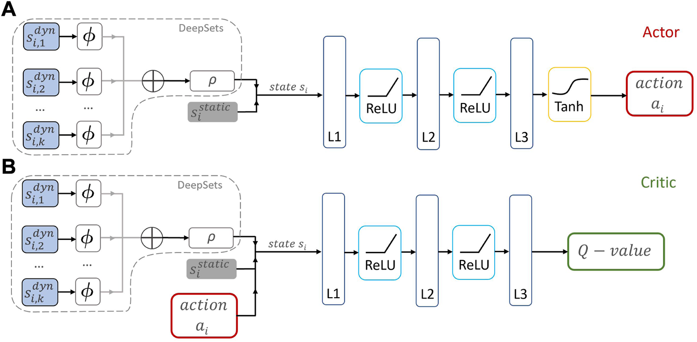
Implementation Architecture. Actor network (A). Critic network (B). Both contain the DeepSets architecture for the scene understanding part of the task. L1, L2 and L3 are fully connected layers, with the respective activation function depicted after each layer. The Critic network additionally takes the action as an input.
The parameters used for the Actor and the Critic networks, as well as the rest of the training details are shown in Table 4. They were obtained by random search with a budget of approximately 500 runs. The configurations used for the search are shown in the last column of Table 4. The rest of the parameters were taken from the original TD3 implementation (Fujimoto et al., 2018).
TABLE 4
| Hyper-parameter | Value | Configuration | |
|---|---|---|---|
| Actor | |||
| Num. neurons per layer | (400, 300, 1) | [100, 200, 300, 400] | |
| Activation functions | (ReLU, ReLU, TanH) | ||
| Policy noise ϵ | |||
| Noise clip c | 0.5 | ||
| Policy delay value d | 2 | ||
| Critic | |||
| Num. neurons per layer | (400, 300, 1) | [100, 200, 300, 400] | |
| Activation functions | (ReLU, ReLU) | ||
| Other | |||
| γ | 0.99 | ||
| τ | 10–4 | ||
| Batch size | 100 | [32, 64, 100, 200] | |
| Learning rate | 10–4 | [10–2, 10–3, 10–4, 10–5] | |
| Max. num. training iterations | 100 K | [102, …, 3*106] |
Training details.
6 Experiments and results
To evaluate the performance of our algorithm we designed a set of realistic highway scenarios on a straight, 3-lane highway 1,000 m long, with a varying number of surrounding vehicles, Nveh = {10, 20, …, 80}, controlled by a simulator (Krajzewicz et al., 2012) policy unknown to the RL agent. For each nveh ∈ Nveh there are 10 scenarios leading to a total of 80 evaluation scenarios, where the surrounding vehicles are positioned randomly along the three-lane highway. In order to capture real highway driving settings as closely as possible, the surrounding vehicles exhibit different driving behaviors within the boundaries of a realistic human driver, i.e., they have different desired velocities, different cooperativeness levels, etc. We let a trained agent navigate through these scenarios and assess its performance in terms of average velocity achieved per set of scenarios for each number of surrounding vehicles. Details regarding the road infrastructure can be found in the code repository in the.xml file named straight.net.xml.
6.1 Comparison to other agents
We compared the performance of our algorithm on the 80 scenarios, against four other driving agents. An IDM-based (Treiber et al., 2000) Sumo-controlled agent, with the same goals as our agent in terms of desired velocity (30 m/s), and parameters concerning driving comfort and aggressiveness levels fit to correspond to the reward function of the RL agent. The parameters can be found in the code repository in the file where the driver behaviors are specified named rou.xml. The Greedy agent builds on the gap-selection approach (Mirchevska et al., 2021) outlined above and simply selects the gap, to which there is a trajectory achieving the highest velocity. The High-Level RL agent is trained to choose from three high-level actions: keep-lane, lane-change to the left or lane-change to the right, and the Gap choosing agent from our previous work (Mirchevska et al., 2021) trained with RL chooses from a proposed set of actions navigating to each of the available gaps. The plot in Figure 5 shows the performance of all agents on the 80 scenarios of varying traffic density. The x-axis represents the number of vehicles per set of scenarios, whereas the average velocity achieved among each 10 varying-density scenarios is read from the y-axis. The shown results for the trained agents are an average of the performance of 10 trained agents. That allows us to show the standard deviation of each of these runs, shown with transparent filled area around the corresponding curve. Low standard deviation indicates that there is small variance between models run with different randomly initialized network weights. Note that after inspection of the scenarios with 50 cars, we determined that there are a few scenarios where the randomly placed surrounding vehicles create a traffic jam and make it difficult for the agents to advance forward. So they are forced to follow the slower leading vehicles, explaining the lower average velocities in that case. Our RL agent has learned to maneuver through the randomly generated realistic highway traffic scenarios without causing collisions and leaving the road boundaries with an average velocity higher than the comparison agents in all traffic densities.
FIGURE 5
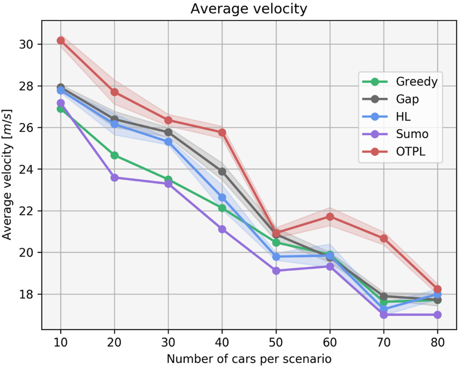
Comparison of the performance of our agent OTPL (red) against the Sumo/IDM-based (purple), Greedy (green), High-Level (blue) and Gap (grey) agents.
6.2 Handling critical scenarios
In order to asses the performance of our agent in critical situations not seen during training, we created two challenging evaluation scenarios. The first one is depicted in Figure 6A, where the vehicle with id 2 suddenly decides to change lane twice (scenes f2 and f3), ending up both times in front of our RL agent driving with high velocity. The RL agent manages to quickly adapt to both situations and avoids collision, finally ending up in the middle free lane, able to advance forward (scene f5).
FIGURE 6
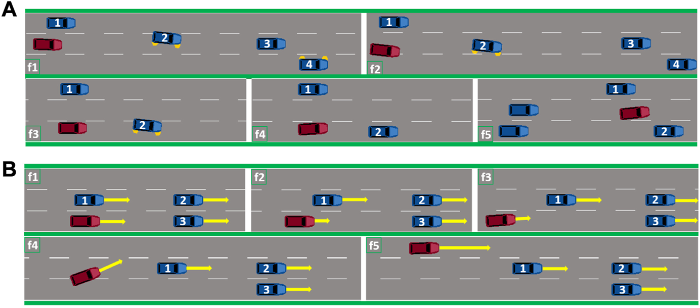
The RL agent (red) in (A) successfully avoids collision when the vehicle 2 decides to cut-in in front of it. The RL agent (red) in (B) learned to perform complex maneuvers consisting of initially slowing down in order to reach the free lane and accelerate towards the desired velocity.
In the second scenario in Figure 6B the RL agent finds itself surrounded by vehicles driving with the same velocity (scene f1), lower than the RL agent’s desired velocity. This situation might occur for, e.g., after the RL agent has entered the highway. In this case, the RL agent has learned to initially slow down (scene f2) and perform a lane-change maneuver (scene f4) towards the free left-most lane. This shows that the RL agent has learned to plan long-term, since slowing down is not beneficial with respect to the immediate reward. The other agents, except the gap-choosing agent were not able to deal with this situation, as they remained in the initial gap until the end. The RL agent’s behavior in these situations can be seen via the link specified in Supplementary Material.
6.3 Smoothness analysis
In this section we are aiming to show whether the ability of the RL agent to directly influence the trajectory through its actions results in smoother driving. We conduct the comparison with respect to the gap agent from our previous work (Mirchevska et al., 2021) that was able to choose a gap to fit into but could not influence the exact trajectory required to reach the gap.
The longitudinal and lateral jerk values are related to the comfort component in driving (Turner and Griffin, 1999; Svensson and Eriksson, 2015; Diels, 2014). Fewer abrupt accelerations/decelerations and smooth lane-changing with well adjusted speed, result in lower jerk values and more comfortable driving experience. In the gap implementation used for the average velocity analysis in Figure 10, the RL agent does not have direct control over the jerk of the trajectories via the reward function. Instead, the underlying trajectory planner chooses the best trajectory in terms of jerk based on an empirically determined jerk cost term combining the longitudinal and the lateral sums of squared jerks. In order to conduct a fair comparison of the performance in terms of average lateral and longitudinal jerk of both the OTPL and the Gap agents, we designed a reward function for the OTPL agent that incorporates the exact jerk cost used for choosing the trajectory in the Gap agent implementation shown in Eq. 8.
Where jcost = jw (sqjlon(a) + sqjlat(a)) is the total jerk cost of the trajectory, js is equal to 1 when and 0 otherwise, where is the empirically determined upper bound value for the total jerk cost used for assigning the jerk-related reward for the chosen trajectory. jrw is a weight value used for adjusting the impact of the jerk reward on the learning and jw is jerk cost weight used to calculate jcost. The rest of the variables used in Eq. 8 are explained in Section 4.3. Further reward function details are accessible in the code repository.
Figures 7A,B show results regarding the average sum of absolute longitudinal and lateral jerk values and the average velocity of the OTPL agent trained with the reward function given in Section 4.3. The performance of six OTPL agents trained with the new reward function from Eq. 8 with different values for jrw, and the gap agent is presented. Note that we use the sum of absolute values for evaluation since significant deviations from 0 in both positive and negative direction are undesired. The results are an average over 5 trained models for each agent. The error bars indicate the standard deviation.
FIGURE 7
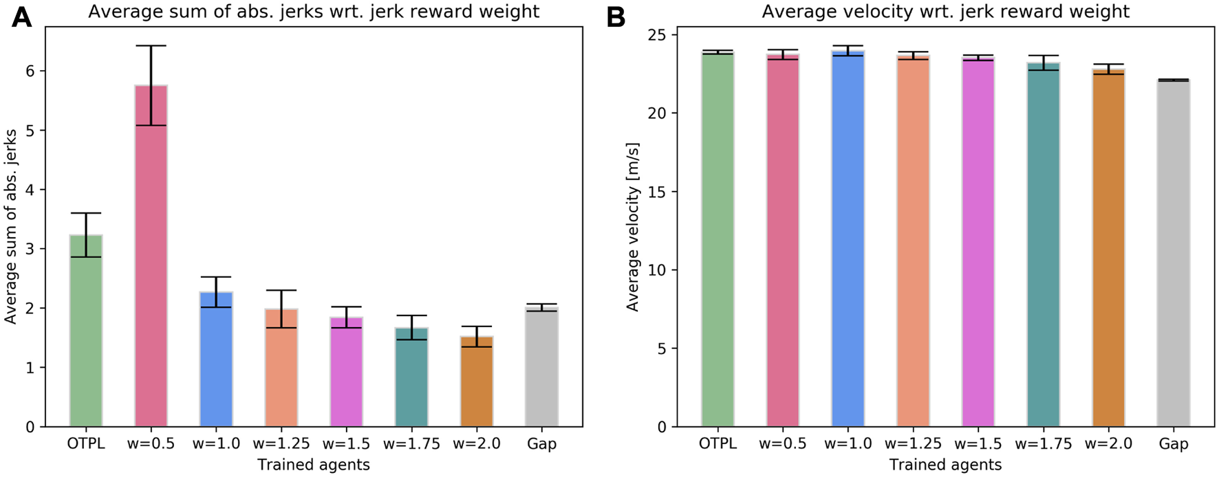
Evaluating the performance in terms of smoothness determined by the jerk values of the chosen trajectories. (A) Average sum of squared jerk values. (B) Average velocity.
The results indicate that the best performance in terms of jerk is yielded when the reward function from Eq. 8 is used and when jrw is assigned a value around 2. However, is important to note that the performance is not very sensitive to the value chosen for jrw and performs similarly well in a range of values. It is interesting to note that when the value for jrw is too low, e.g., 0.5, the agent deems the jerk-related reward component less significant which results in higher jerk values. On the other end of the spectrum, for weight values higher than 2, the performance slowly becomes more conservative and the velocity decreases. In this case, the agent assigns more significance to low jerk values which leads to avoiding lane-changes and acceleration. The performance of the OTPL agent that was trained with the reward function from Eq. 7, depicted first with light green, shows that the reward function is less sensitive to the smoothness component and hence results in slightly worse performance in terms of jerk. It is worthy highlighting that this increase in performance in terms of smoothness of the agents trained with the reward function in Eq. 8, comes at almost no cost regarding the average velocity as shown in Figure 7B. The agents that are trained with the reward function that incorporates the jerk cost of the trajectory, drive smoother than the gap agent that does not have an influence over this component.
The performance in terms of smoothness of the good agents trained with the reward function in Eq. 8, according to the research presented in Turner and Griffin (1999); Svensson and Eriksson (2015); Diels (2014), falls into the range of smooth and comfortable driving. For reference, a value of zero is accomplished only if the vehicle does not move, or it drives in its own lane with constant longitudinal and lateral velocities for the whole duration of the scenarios.
6.4 Lateral and longitudinal trajectory duration analysis
To ensure that our agent fully utilizes the flexibility of being able to choose any continuous value between 1 and 6 s for both the duration of the longitudinal and the lateral trajectory profiles, we have included a plot in Figure 8 that displays the frequency of occurrence of longitudinal (A) and lateral (B) trajectories within 5 different duration ranges. The plots show that the agent learned to combine the longitudinal and lateral trajectory durations in various ways while optimizing for velocity and smoothness. This can be seen in Figure 8B where the agent avoids choosing trajectories that perform lateral movement in a duration of 1–2 s since this would result in high lateral jerk in most cases. At the same time, in Figure 8A can be seen that the agent rarely prefers choosing trajectories with longer durations, since they are slower in reaching the final velocity.
FIGURE 8
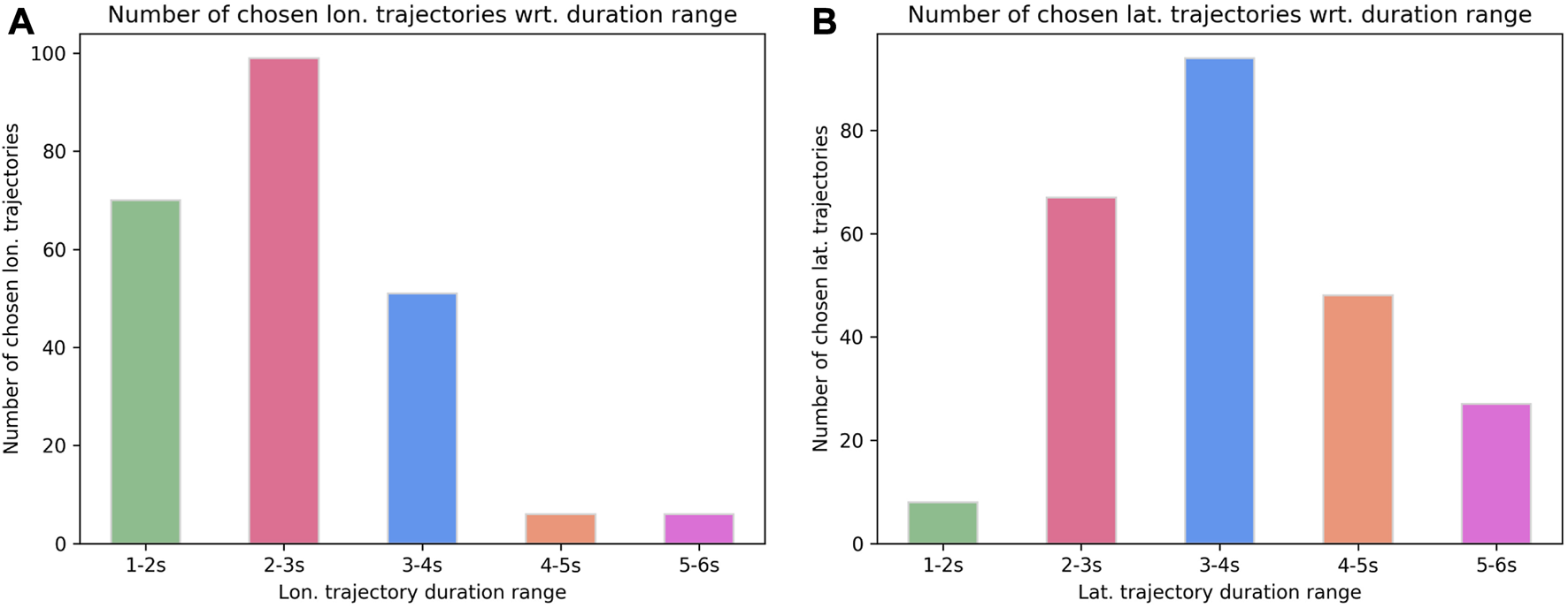
How often does the trained OTPL agent choose trajectories from the duration ranges shown on the x-axis, longitudinally (A) and laterally (B).
Once we confirmed that the agent has effectively learned to take advantage of the continuous range when selecting longitudinal and lateral trajectory durations, we proceeded to conduct an additional experiment to evaluate whether the agent indeed gains a benefit from this capability.
For that purpose, we trained models with fixed, discrete trajectory durations, same for the lateral and the longitudinal component, ranging from 2 to 6 s. We show average of 3 trained models for each agent, while all models were trained with the reward function from Eq. 7. As shown in Figure 9, none of these models was able to perform as good as the OTPL agent in terms of velocity and smoothness. Additionally, some of the models, also experienced failures more often since in certain situations a specific trajectory with non-equal and non-discrete longitudinal and lateral profile durations is required to avoid an accident or to avoid exiting the road boundaries. For too short trajectory durations, such as 2s, despite the good performance wrt. velocity, the agent learned to produce high-jerk trajectories and fails in 20/80 scenarios. As the duration goes towards 6 s, smoother trajectories are learned, but with lower speeds. The number of fails decreases as well. In these cases, since the performance in terms of velocity is also weaker, the agent learned to keep the lane most of the time. This indicates that the flexibility that the OTPL agent is provided with in terms of selecting the durations of both trajectory profiles, plays an important role in the overall performance.
FIGURE 9
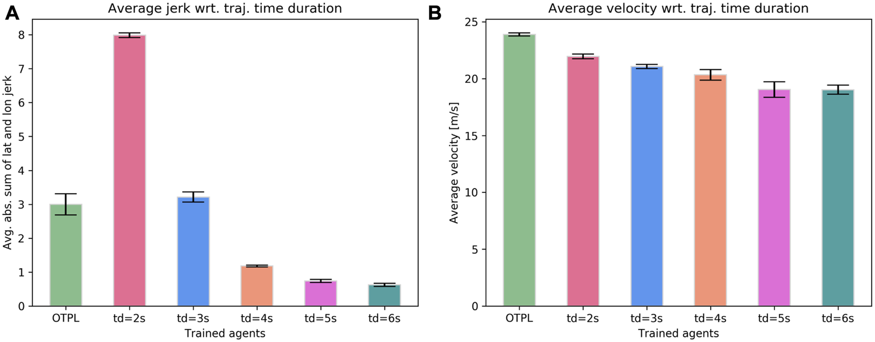
Performance comparison between the OTPL agent and the agents trained with fixed discrete trajectory durations, same for the longitudinal and the lateral profiles in terms of average sum of absolute lateral and longitudinal (A) jerks and average velocity (B).
7 Training data analysis
Since we are training the agent on a fixed batch of offline data and it does not get to explore the environment based on the current policy, the quality of the data is of significant importance. We performed data analysis to investigate the benefits of the structure imposed by the trajectory polynomials during data collection for the learning progress. Additionally, we provide analysis of how the percentage of negative training samples affects the learning.
7.1 Importance of structured data generation
A common way of approaching the highway driving task with online RL is teaching an agent to perform low-level actions over small time-step intervals. Since we are interested in offline RL, in order to evaluate its performance, we randomly collected data with an agent that chooses throttle and steering wheel actions each 0.2 s. In addition to other tasks, in this case the agent has to learn not to violate the maximum steering angle, i.e., not to start driving in the opposite direction, as well as not to violate the acceleration constraints. As a consequence, the collected data consisted of a large portion of such samples, whereas the number of non-terminal and useful samples was negligible. Additionally, the agent was never able to achieve high velocities since it was interrupted by some of the more likely negative outcomes (like constraint violations) before being able to accelerate enough. The agent trained using the aforementioned data did not learn to avoid the undesired terminal states while driving. Relying on the structure imposed by the polynomial trajectory generation, helps to obtain high-quality data for offline learning.
7.2 Percentage of transitions towards a terminal state
When it comes to terminal states resulting in negative reward, in our case the agent needs to learn to avoid collisions with other vehicles and to stay within the road boundaries. (Terminal state occurs when the end of the road is reached as well but reaching that terminal state is not being punished since it does not depend on the agent’s behavior.) We observed that the frequency of data sequences that end in such terminal states and the complexity of the task play a critical role in the performance of the trained agent. Our results show, for instance, that the agent learns to not leave the road very quickly and from much more limited data compared to the more complex collision avoidance task (4% of data with samples of leaving the road vs. of data with samples of collisions).
Figures 10A,B show the average performance of 5 agents trained with different percentages of terminal samples in the training data. In (A) the y-axis shows the average velocity achieved in the evaluation scenario (randomly generated, 50 surrounding vehicles), depending on the portion of terminal states in the data (x-axis). Figure 10B represents the driving time of each of the agents. Note that the agent trained without any terminal samples never learned to avoid collisions, so it only endures 5 s before it collides. The rest of the agents, learn not to collide and are able to complete the scenario. The conclusion is, if there are too few terminal samples, the agent never learns to avoid collisions (in the 0% case), since it is not aware of that occurrence. If there are to many, the agent has problems learning to achieve high velocities, since it has learned to be more conservative. The best performance is achieved when of the training samples are terminal.
FIGURE 10
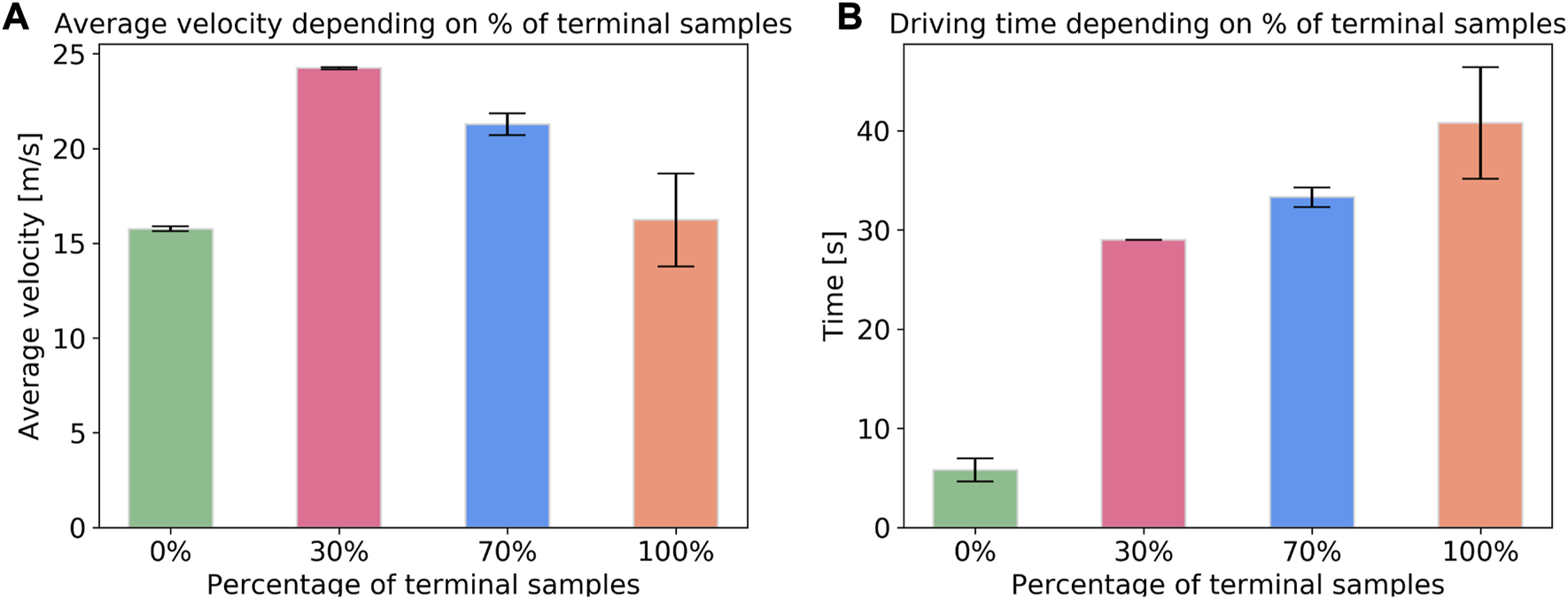
Importance of the percentage of negative samples in the training data shown wrt. average speed (A) and driving time (B). The bars are showing the mean over 5 trained agent for each percentage. The error bars indicate the standard deviation.
8 Conclusion
In this study, we address the challenge of training a RL agent to navigate realistic and dynamic highway scenarios by optimizing trajectory parameters. Our actor-critic based agent learns to generate four continuous actions describing a trajectory that is generated by an underlying polynomial-based trajectory generation module. Trained on a fixed batch of offline data gathered with a basic random collection policy, our agent successfully navigates randomly generated highway scenarios with varying traffic densities, outperforming comparison agents in terms of average speed. In addition to avoiding collisions and staying within the road boundaries, our agent learns to execute complex maneuvers in critical situations. Furthermore, we analyze the effect of training data composition on the performance of the RL policy learned in the offline case. We propose an alternative reward function for the OTPL agent that directly maps the cost function used to select the best trajectories in terms of jerk in the Gap agent implementation, allowing us to conduct smoothness and comfort analyses. Our findings show that having direct control through the reward function over trajectory selection leads to smoother driving.
Finally, we train models with discrete, fixed trajectory durations and compare their performance to that of the OTPL agent, demonstrating the importance of the ability to choose from a continuous range of values for both the longitudinal and lateral trajectory profiles in achieving superior performance.
Statements
Data availability statement
The datasets presented in this study can be found in online repositories. The names of the repository/repositories and accession number(s) can be found below: https://nrgit.informatik.uni-freiburg.de/branka.mirchevska/offline-rl-tp/-/tree/main/training_data.
Author contributions
As the main author, BM designed the objective to learn target trajectory values as actions, in a Reinforcement Learning framework equipped with an underlying trajectory planner. Additionally, provided the code base, designed the experimental framework, performed all experiments and wrote the paper. MW played a significant role in the conceptualization of the idea and the problem formalization, provided supervision and feedback for the paper. JB regularly supervised the findings throughout the course of this work and provided consultation for refining the paper.
Funding
BM is funded through the State Graduate Funding Program of Baden-Württemberg. JB’s contribution is supported by BrainLinks-BrainTools which is funded by the Federal Ministry of Economics, Science and Arts of Baden-Württemberg within the sustainability program for projects of the excellence initiative II. For the publication of this work we acknowledge support by the Open Access Publication Fund of the University of Freiburg.
Acknowledgments
We would like to thank Maria Kalweit, Gabriel Kalweit and Daniel Althoff for the fruitful discussions on offline RL and trajectory planning.
Conflict of interest
Author MW was employed by company BMW Group.
The remaining authors declare that the research was conducted in the absence of any commercial or financial relationships that could be construed as a potential conflict of interest.
Supplementary material
The Supplementary Material for this article can be found online at: https://www.frontiersin.org/articles/10.3389/ffutr.2023.1076439/full#supplementary-material
Footnotes
1.^Known as offline or fixed-batch RL.
2.^In the sense that they are generated with different traffic densities, the surrounding vehicles are modeled with various behaviors, have different goals, all of which is unknown to the agent in advance, much like real highway traffic.
3.^Terminal samples refer to instances in which the agent reaches a state from which it cannot continue, typically due to an undesired behavior.
4.^We found that in contrast to Double Q-learning, using three critics improves the performance.
5.^The lateral and longitudinal acceleration and lateral velocity are equal to 0, when the vehicle drives straight keeping its current velocity.
6.^Rate of change of acceleration wrt. time.
References
1
Bellegarda G. Byl K. (2019). Combining benefits from trajectory optimization and deep reinforcement learning. CoRR abs/1910.09667.
2
Bogdanovic M. Khadiv M. Righetti L. (2021). Model-free reinforcement learning for robust locomotion using trajectory optimization for exploration. CoRR abs/2107.06629.
3
Borrelli F. Falcone P. Keviczky T. Asgari J. Hrovat D. (2005). Mpc-based approach to active steering for autonomous vehicle systems. Int. J. Veh. Aut. Syst.3, 265–291. 10.1504/ijvas.2005.008237
4
Claussmann L. Revilloud M. Gruyer D. Glaser S. (2019). A review of motion planning for highway autonomous driving. IEEE Trans. Intelligent Transp. Syst.21, 1826–1848. 10.1109/tits.2019.2913998
5
Diels C. (2014). Will autonomous vehicles make us sick. Contemp. ergonomics Hum. factors, 301–307.
6
Falcone P. Borrelli F. Asgari J. Tseng H. E. Hrovat D. (2007). Predictive active steering control for autonomous vehicle systems. IEEE Trans. Control Syst. Technol.15, 566–580. 10.1109/tcst.2007.894653
7
Fujimoto S. van Hoof H. Meger D. (2018). “Addressing function approximation error in actor-critic methods,” in Proceedings of the 35th international conference on machine learning, ICML 2018 (Stockholm, Sweden: Stockholmsmässan), 1582–1591.
8
Glaser S. Vanholme B. Mammar S. Gruyer D. Nouvelière L. (2010). Maneuver-based trajectory planning for highly autonomous vehicles on real road with traffic and driver interaction. IEEE Trans. Intelligent Transp. Syst.11, 589–606. 10.1109/TITS.2010.2046037
9
Grigorescu S. Trasnea B. Cocias T. Macesanu G. (2020). A survey of deep learning techniques for autonomous driving. J. Field Robotics37, 362–386. 10.1002/rob.21918
10
Hoel C.-J. Wolff K. Laine L. (2018). “Automated speed and lane change decision making using deep reinforcement learning,” in 2018 21st international conference on intelligent transportation systems (ITSC), 2148–2155. 10.1109/ITSC.2018.8569568
11
Hoel C. Driggs-Campbell K. R. Wolff K. Laine L. Kochenderfer M. J. (2019). Combining planning and deep reinforcement learning in tactical decision making for autonomous driving. CoRR abs/1905.02680.
12
Huegle M. Kalweit G. Werling M. Boedecker J. (2020). “Dynamic interaction-aware scene understanding for reinforcement learning in autonomous driving,” in 2020 IEEE international conference on robotics and automation (ICRA), 4329–4335. 10.1109/ICRA40945.2020.9197086
13
Hugemann W. (2002). Driver reaction times in road traffic.
14
Hügle M. Kalweit G. Mirchevska B. Werling M. Boedecker J. (2019). “Dynamic input for deep reinforcement learning in autonomous driving,” in 2019 IEEE/RSJ international conference on intelligent robots and systems (IROS), 7566–7573.
15
Kalweit G. Huegle M. Werling M. Boedecker J. (2020). “Deep inverse q-learning with constraints,”. Advances in neural information processing systems. Editors LarochelleH.RanzatoM.HadsellR.BalcanM.LinH. (Curran Associates, Inc.), 14291–14302. Available at: https://nips.cc/virtual/2020/public/poster_a4c42bfd5f5130ddf96e34a036c75e0a.html.
16
Kalweit G. Huegle M. Werling M. Boedecker J. (2021). “Q-learning with long-term action-space shaping to model complex behavior for autonomous lane changes,” in 2021 IEEE/RSJ International Conference on Intelligent Robots and Systems (IROS), Prague, Czech Republic, September 27–October 1, 2021. (IEEE), 5641–5648. 10.1109/IROS51168.2021.9636668
17
Katrakazas C. Quddus M. Chen W.-H. Deka L. (2015). Transportation research Part C: Emerging technologies.Real-time motion planning methods for autonomous on-road driving: State-of-the-art and future research directions
18
Kaushik M. Prasad V. Krishna M. Ravindran B. (2018). Overtaking maneuvers in simulated highway driving using deep reinforcement learning, 1885–1890. 10.1109/IVS.2018.8500718
19
Kendall A. Hawke J. Janz D. andDaniele Reda P. M. Allen J. Lam V. et al (2018). Learning to drive in a day. CoRR abs/1807.00412.
20
Krajzewicz D. Erdmann J. Behrisch M. Bieker-Walz L. (2012). Recent development and applications of sumo - simulation of urban mobility. Int. J. Adv. Syst. Meas.3and4.
21
Kuutti S. Bowden R. Jin Y. Barber P. Fallah S. (2021). A survey of deep learning applications to autonomous vehicle control. IEEE Trans. Intelligent Transp. Syst.22, 712–733. 10.1109/tits.2019.2962338
22
Levine S. Kumar A. Tucker G. Fu J. (2020). Offline reinforcement learning: Tutorial, review, and perspectives on open problems.
23
Meurer A. Smith C. P. Paprocki M. Čertík O. Kirpichev S. B. Rocklin M. et al (2017). Sympy: Symbolic computing in python. PeerJ Comput. Sci.3, e103. 10.7717/peerj-cs.103
24
Mirchevska B. Blum M. Louis L. Boedecker J. Werling M. (2017). “Reinforcement learning for autonomous maneuvering in highway scenarios,” in 11 Workshop Fahrerassistenzsysteme und automatisiertes Fahren.
25
Mirchevska B. Hügle M. Kalweit G. Werling M. Boedecker J. (2021). Amortized q-learning with model-based action proposals for autonomous driving on highways. In 2021 IEEE international conference on robotics and automation (ICRA). 1028–1035. 10.1109/ICRA48506.2021.9560777
26
Mirchevska B. Pek C. Werling M. Althoff M. Boedecker J. (2018). “High-level decision making for safe and reasonable autonomous lane changing using reinforcement learning,” in 2018 21st international conference on intelligent transportation systems (ITSC), 2156–2162.
27
Mukadam M. Cosgun A. Nakhaei A. Fujimura K. (2017). “Tactical decision making for lane changing with deep reinforcement learning,” in NIPS workshop on machine learning for intelligent transportation systems.
28
Nageshrao S. Tseng H. E. Filev D. (2019). “Autonomous highway driving using deep reinforcement learning,” in 2019 IEEE international conference on systems, man and cybernetics (SMC), 2326–2331.
29
Ota K. Jha D. K. Oiki T. Miura M. Nammoto T. Nikovski D. et al (2019). “Trajectory optimization for unknown constrained systems using reinforcement learning,” in 2019 IEEE/RSJ international conference on intelligent robots and systems (IROS), 3487–3494.
30
Rao A. (2010). A survey of numerical methods for optimal control. Adv. Astronautical Sci.135.
31
Ronecker M. P. Zhu Y. (2019). Deep q-network based decision making for autonomous driving. 2019 3rd international conference on robotics and automation sciences (ICRAS), 154–160.
32
Saxena D. M. Bae S. Nakhaei A. Fujimura K. Likhachev M. (2019). Driving in dense traffic with model-free reinforcement learning. CoRR abs/1909.06710.
33
Schwarting W. Alonso-Mora J. Rus D. (2018). Planning and decision-making for autonomous vehicles.
34
Sutton R. S. Barto A. G. (2018). Reinforcement learning: An introduction. second edn. The MIT Press.
35
Svensson L. Eriksson J. (2015). Tuning for ride quality in autonomous vehicle: Application to linear quadratic path planning algorithm.
36
Treiber M. Hennecke A. Helbing D. (2000). Congested traffic states in empirical observations and microscopic simulations. Phys. Rev. E62, 1805–1824. 10.1103/physreve.62.1805
37
Turner M. Griffin M. J. (1999). Motion sickness in public road transport: The effect of driver, route and vehicle. Ergonomics42, 1646–1664. 10.1080/001401399184730
38
Wang J. Zhang Q. Zhao D. Chen Y. (2019a). Lane change decision-making through deep reinforcement learning with rule-based constraints. CoRR abs/1904.00231
39
Wang P. Chan C.-Y. de La Fortelle A. (2018). A reinforcement learning based approach for automated lane change maneuvers.
40
Wang P. Li H. Chan C.-Y. (2019b). Quadratic q-network for learning continuous control for autonomous vehicles.
41
Wang S. Jia D. Weng X. (2019c). Deep reinforcement learning for autonomous driving.
42
Werling M. Ziegler J. Kammel S. Thrun S. (2010). “Optimal trajectory generation for dynamic street scenarios in a frenét frame,” in 2010 IEEE international conference on robotics and automation.
43
Xu W. Wei J. Dolan J. M. Zhao H. Zha H. (2012). “A real-time motion planner with trajectory optimization for autonomous vehicles,” in 2012 IEEE international conference on robotics and automation.
Appendix
Trajectory generation details
As mentioned in Section 3.3, we use quartic and quintic polynomials to describe the longitudinal and the lateral trajectory components, respectively. Fourth and fifth order polynomials were chosen for the longitudinal and lateral movement components, respectively, due to their ability to model complex trajectories with sufficient accuracy while striking a good balance between complexity and descriptive power. More precisely, we need to solve Appendix Eqs. 1, 2 in order to get the positions wrt. time for the desired trajectory. In order to do that, we need the values for the coefficients b3, b4, c3, c4 and c5, which considering the parameters given in Table A1, we can get by solving the systems of equations shown in Appendix Eqs. 3, 4. Once we have the positions for the complete duration of the trajectory, we can get the velocities, accelerations and jerk values, by calculating first, second and third derivative of the position wrt. the time t. For time-step size we use dt = 0.2s.For predicting the behavior of the surrounding vehicles we assume constant velocity trajectories and use them for collision checking with the trajectory of the RL agent. Deviations from the predictions of the other vehicles are handled in an on-line fashion.
TABLE A1
| Parameter/Coefficient | Description |
|---|---|
| b 0 | current longitudinal position |
| b 1 | current longitudinal velocity |
| b 2 | current longitudinal acceleration |
| acc lon | target longitudinal acceleration = 0 |
| c 0 | current lateral position |
| c 1 | current lateral velocity |
| c 2 | current lateral acceleration |
| vel lat | target lateral velocity = 0 |
| acc lat | target lateral acceleration = 0 |
Polynomial parameters.
Action target velocity boundaries
As outlined in Section 5.1, we derive a formula based on which, given the current state and we calculate the minimum and maximum target velocity values the agent is able to choose from. This is done so that the generated trajectory will not violate the minimum/maximum possible longitudinal acceleration. This contributes for collection of data that consists of informative samples that enable fast learning of a good policy, instead of data-samples that are repetitive and lack useful information.
Additionally, this way we avoid learning the minimum/maximum acceleration constraint, which simplifies the learning process. By calculating the second derivative of Appendix Eq. 1, we get the trajectory acceleration equation.By calculating the first derivative of the acceleration equation and setting it to 0, we get the expression for obtaining its minimum/maximum.After solving for t we get the time-step at which the minimum/maximum acceleration is achieved. We substitute the expression for t back to the acceleration in Appendix Eq. 5 and we set it to the known minimum/maximum acceleration value. After finding the solutions for b3 and b4 using Appendix Eqs. 5, Eq. 6, we can substitute them in Appendix Eq. 3 and express the values for the minimum and maximum atv allowed. We use Simpy (Meurer et al., 2017) to solve the equation and get the final values for the minimum and the maximum allowed velocities.
Summary
Keywords
reinforcement learning, trajectory optimization, autonomous driving, offline reinforcement learning, continuous control
Citation
Mirchevska B, Werling M and Boedecker J (2023) Optimizing trajectories for highway driving with offline reinforcement learning. Front. Future Transp. 4:1076439. doi: 10.3389/ffutr.2023.1076439
Received
16 November 2022
Accepted
27 March 2023
Published
12 May 2023
Volume
4 - 2023
Edited by
Michele Segata, University of Trento, Italy
Reviewed by
Shobha Sundar Ram, Indraprastha Institute of Information Technology Delhi, India
Reinis Cmurs, Robert Bosch (Germany), Germany
Updates
Copyright
© 2023 Mirchevska, Werling and Boedecker.
This is an open-access article distributed under the terms of the Creative Commons Attribution License (CC BY). The use, distribution or reproduction in other forums is permitted, provided the original author(s) and the copyright owner(s) are credited and that the original publication in this journal is cited, in accordance with accepted academic practice. No use, distribution or reproduction is permitted which does not comply with these terms.
*Correspondence: Branka Mirchevska, mirchevb@informatik.uni-freiburg.de
This article was submitted to Connected Mobility and Automation, a section of the journal Frontiers in Future Transportation
Disclaimer
All claims expressed in this article are solely those of the authors and do not necessarily represent those of their affiliated organizations, or those of the publisher, the editors and the reviewers. Any product that may be evaluated in this article or claim that may be made by its manufacturer is not guaranteed or endorsed by the publisher.