Validation of MCMC-Based Travel Simulation Framework Using Mobile Phone Data

An essential step in agent-based travel demand models is the characterization of the population, including transport-related attributes. This study looks deep into various mobility data in the province of Liège, Belgium. Based on the data stemming from the 2010 Belgian HTS, that is, BELDAM, a Markov chain Monte Carlo (MCMC) sampling method combined with a cross-validation process is used to generate sociodemographic attributes and trip-based variables. Besides, representative micro-samples are calibrated using data about the population structure. As a critical part of travel demand modeling for practical applications in the real-world context, validation using various data sources can contribute to the modeling framework in different ways. The innovation in this study lies in the comparison of outputs of MCMC with mobile phone data. The difference between modeled and observed trip length distributions is studied to validate the simulation framework. The proposed framework infers trips with multiple attributes while preserving the traveler’s sociodemographics. We show that the framework effectively captures the behavioral complexity of travel choices. Moreover, we demonstrate mobile phone data’s potential to contribute to the reliability of travel demand models.

Introduction

Travel Demand Modeling

Travel behavior research aims at understanding how people build their travel choice sets, which include essential elements such as trip purpose, departure time, travel distance, activity location, activity duration, and participants engaged in ongoing activities. These elements assume a definition of activity given by a set of persons interacting with each other (Axhausen, 2007). Multiple predictive travel demand models have been developed to support firms’ and governments’ decision-making. In the last decades, advanced models have grown with the technology available and improved the understanding of human activity-travel patterns. One of the most important travel demand modeling changes is the evolution from the trip- to activity-based models (Anda et al., 2017). Preference is given to activity-based models, mainly due to their ability to describe travel behavior’s disaggregated nature. In activity-based approaches, a typical human’s daily schedule that belongs to a particular behavior class is reproduced (Bazzan and Klügl, 2014). Agent- and activity-based approaches perfectly fit together as an agent-based approach uses models for explicit individual decisions and enables a wider range of transportation policies. Compared with classical four-step trip-based models, agent-based activity-based models require a synthetic population as a critical input (Borysov et al., 2019; Ramadan and Sisiopiku, 2019; Hörl and Balac, 2020). The expected output contains a set of agents with corresponding sociodemographic (e.g., occupation and income) and urban transport–related (e.g., travel mode choice and activity location) characteristics.

Problem Statement

Despite the increasing availability of new big data sources, transport demand models used in planning practice still heavily rely on traditional data sources such as travel diary surveys and population censuses (Anda et al., 2017). The main advantage of travel surveys is the detailed description of anonymous individuals’ sociodemographics and daily travel plans. Meanwhile, censuses and the national register offer a very refined spatial resolution of population distribution. Household travel surveys (HTSs) and censuses conducted by government agencies can provide a sample for research purposes. However, they are usually updated at a low temporal frequency owing to the high cost. In contrast, new big data sources such as mobile phone records and smart card data possess higher penetration rates of the real population, and the data can be collected at a lower cost (Rojas et al., 2016; Li et al., 2018). However, due to privacy issues, they are hardly available to researchers in their natural form. The most impactful limitation of new big data is the minimal availability of individuals’ sociodemographics. Lack of user information makes the household travel survey data indispensable during the travel demand modeling.

Nonetheless, some studies have shown the tremendous potential in applying the new big data sources combined with the traditional data sources to exploit agent-based activity-based models’ capabilities. Medina and Erath (2013) combined public transport smart card transaction data, travel diary surveys, and building information data sources to generate the initial transport demand concerning dynamic workplace capacities. They used the smart card data to detect the number of workers at each stop and each work schedule within Singapore. Unlike the smart card data that focus on public transport, mobile phone data have a broader deployment in the transport planning community. Two main mobile phone data sources in terms of collection systems and techniques have been applied in travel behavior research: cellular network–based and smartphone sensor–based (Wang et al., 2018). The first one’s event-driven data are collected when mobile communication or Internet usage occurs, according to which telecom companies generate call detail records (CDRs) for billing. Researchers have expanded the use of CDR data, ranging from travel demand modelings, such as population generation (Zilske and Nagel, 2015; Bassolas et al., 2019; Franco et al., 2020), to the understanding of human mobility patterns (González et al., 2008; Yan et al., 2017) and origin–destination (OD) matrix creation (Iqbal et al., 2014; Goulding, 2018). Smartphone sensor–based data are generally conducted through public mobile phone applications (e.g., Google) developed by third parties to provide location-based services (Kang et al., 2020; Kraemer et al., 2020). Both mobile phone data types are produced anonymously and are ordinarily available for special research purposes. Mobile phone data serve not only the domain of model calibration but also validation due to their reliability. Liu et al. (2014) used mobile phone data to build a validation measure for activity-based transportation models. They considered the average length of activity sequences generated from mobile phone data as the validation measure for the activity-travel sequences that stem from traditional activity-travel surveys. Unfortunately, no official travel surveys had been conducted for the study region in the time frame of Liu et al. (2014), necessitating the use of two other countries’ travel surveys to examine the validation potential of mobile phone data. Nonetheless, their study suggests that the derived home-based tour profile and daily-sequence profile have high correlation coefficients with those drawn from a real travel survey. This study’s main contribution lies in validating Markov chain Monto Carlo (MCMC) simulation–based outputs using mobile phone data within the same geographical cover. In particular, the study looks deep into multiple data sources to predict trip length distributions and compares these with the ones derived from mobile phone data.

Population Synthesis

The MCMC simulation–based approach has been proposed by Farooq et al. (2013) to generate a synthetic population matching the observed population. Farooq et al. (2013) used the real population from the Swiss census to compare the performance of Gibbs sampling with that of the standard iterative proportional fitting (IPF). The standardized root mean squared error (SRMSE) statistic, an indicator that assesses the goodness of fit of the synthetic data (Zhu and Ferreira, 2014), indicates that even the worst case (with three out of four incomplete conditionals) simulation-based synthesis (SRMSE = 0.35) outperforms the best case IPF synthesis (SRMSE = 0.64). An extended hidden Markov model (HMM)–based approach has been presented to reproduce the marginal distributions and their corresponding multivariate joint distributions with an acceptable error rate (SRSME = 0.54 for six attributes) (Saadi et al., 2016a). A comparison of the HMM with IPF illustrates the advantages of the HMM over IPF for small sample sizes (<25% population) in terms of SRMSE. Since MCMC requires preparing the full conditional distributions, which is complicated, the Bayesian network has been considered an alternative tool to simplify the joint distribution estimation (Sun and Erath, 2015). The proposed Bayesian network model looks deeply into the size of parameters regarding the trade-off between model complexity and robustness. Again, they adopt the popular measure, SRMSE, to assess the performance of existing population synthesis techniques, including IPF, MCMC, and the Bayesian network. IPF and MCMC begin to outperform the Bayesian network approach when the total population’s sampling rate is over 40%. The overfitting problem appears for IPF and MCMC when the training data are not fully representative of the underlying relationship. However, this is not a case for the Bayesian network even with, for example, 1% population (Sun and Erath, 2015). The other advantage of the Bayesian network given by Sun and Erath (2015) is its flexibility when it comes to configuring hierarchical household structure, which is not investigated in this study.

Of note here is that the sampling rate in the population synthesis approaches mentioned above has played a crucial role in the assessment procedure caused by the lack of data. While the whole dataset is rarely available for research, except for Farooq et al. (2013), the other two approaches (Sun and Erath, 2015; Saadi et al., 2016a) assumed that the travel survey data present the full population. After that, Public Use Micro Sample (PUMS) data are randomly extracted from the travel survey as test datasets for simulation under different sampling rates (e.g., ranging from 1 to 100%). If the sampling rate is relatively low, it is easy to extract data that are not representative enough from the travel survey with fluctuating uncertainty, limiting the use of the travel survey data.

Research Contributions

The necessity of introducing new data sources to validate synthetic outputs has been manifested. Since this study focuses on the trip length distribution as a validation measure using mobile phone data and the comparison of various population synthesis approaches is not within this study’s scope, we choose MCMC, that is, the Gibbs sampler, to estimate the actual travel demand. The choice is made as the Gibbs sampler features a higher level of heterogeneity due to its flexibility using various data sources at different spatial scales and scalability regarding the number of synthesized attributes (Farooq et al., 2013). A k-fold cross-validator will compensate the simulation for the risk of overfitting caused by full conditional distributions when a high sampling rate of travel survey data is chosen in our practice.

As we mentioned in the introduction, travel behavior research aims to understand how people build their travel choice sets. The existing investigations tend to focus on activity sequence characterization. Subsequently, the obtained sequences and their implicit travel episodes can serve as a critical input for travel demand analysis and forecasting (Liu et al., 2015). Saadi et al. (2016b) integrated the MCMC population synthesis approach with a profiling method to describe and assign activity sequences to the synthetic individuals. Data stemming from the 2010 Belgian daily HTS, that is, BELDAM, are used to calibrate the integration. This integrated approach’s main limitation is a lack of travel time information crucial for activity sequences. Moreover, the choice of activity location, travel distance, and transport modes will have to be further made to build a complete daily activity plan. Indeed, it is common for travel demand modeling to generate populations and related daily activities first and then design different travel behavior choice sets (Arentze and Timmermans, 2004; Roorda et al., 2008; Habib, 2018). This study chooses other trip elements to describe travel behavior compared with Saadi et al. (2016b), including agents’ trip motivation, start time, travel duration, travel distance, mode choice, and activity duration. Instead of preparing the synthetic population and trip plans separately, the model predicts which trips are conducted by whom, when, which modes, and how far within a typical day at the same time. After that, we use large-scale mobile phone OD matrices of the province of Liège, Belgium, for validation by comparing the synthetic and observed trip length distributions.

The article’s remainder is organized as follows: we first describe the data obtained from the 2010 Belgian national HTS, that is, BELDAM, and the mobile phone data provided by Wallonia SPW Mobilité et Infrastructures. Following data description, we introduce the modeling framework to address the problem. Then, the results are presented in the following section. Finally, we discuss the key features of the proposed approach and formulate the conclusions.

Data

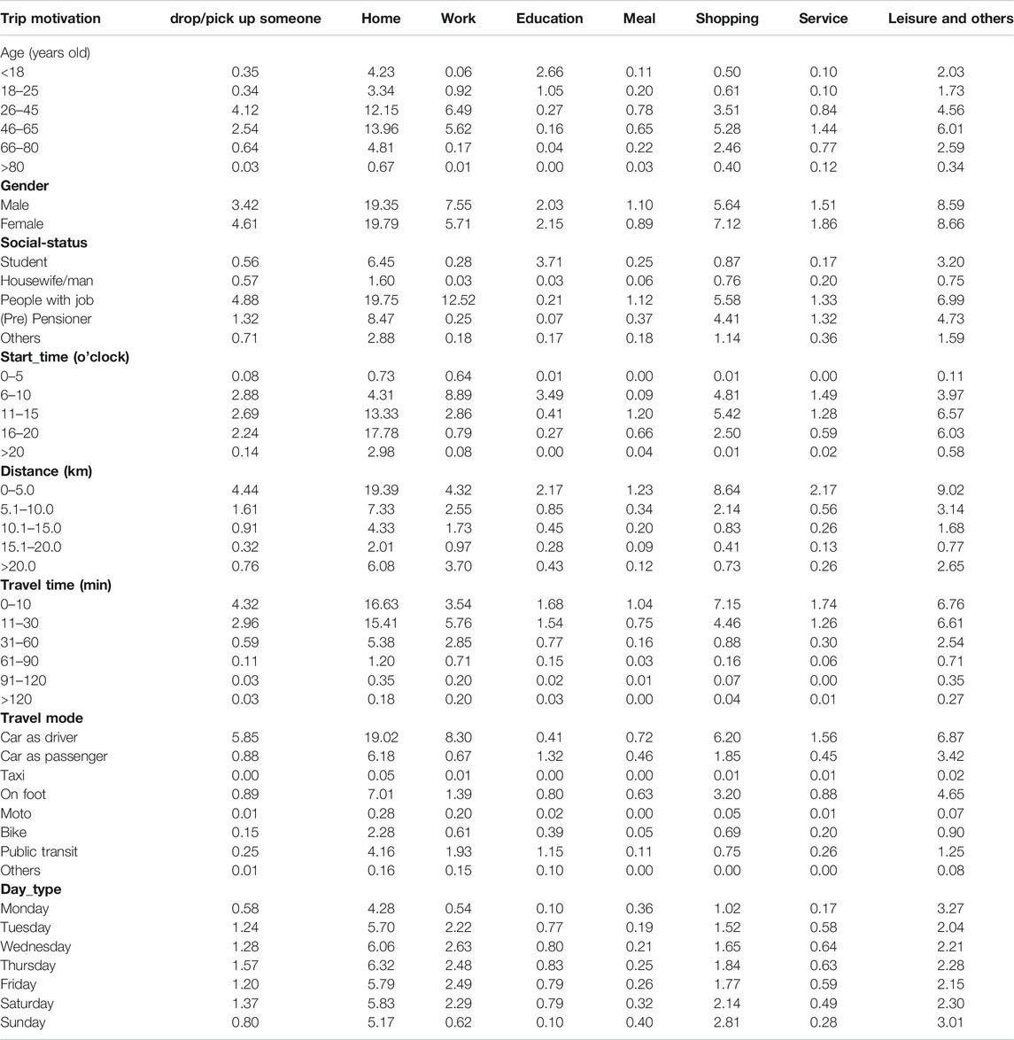
We use three primary data sources (Table 1) to investigate the population’s daily activity-travel behaviors. The first source is the Belgian HTS, that is, BELDAM. After the data cleaning and preprocessing, daily travel plans are prepared, including 8,685 respondents and 29,357 trips across the country. Each entry of the data contains a trip’s elements (e.g., trip motivation, start time, travel duration, travel distance, mode choice, and activity duration) and the corresponding individual’s sociodemographics (e.g., age, gender, and socio-professional status). Supplementary Table S1 gives us a glance at the discrete distributions of variables of interest. It tells the story of population activities, that is, more people aged between 26 and 45 years have drop/pick-up activity than other age groups. Generally, people who are 26–45 years old can be parents and employees at the same time, which can explain why people with a job take more drop/pick-up activity than other groups in Supplementary Table S1. Other phenomena such as more males going to work and more females going shopping are presented as well. Besides, the most popular time frame for commuting or going to school is from six to ten o’clock, and activities people seem to prefer taking lunch outside other than breakfast and dinner. Another well-known truth is that people travel more by cars than other travel modes.

TABLE 1

TABLE 1. Comparison of three data sources.

The second data source is the population’s structure by place of residence, age, and gender from STATBEL, the Belgian statistical office. The data are available at the municipality level. As the mobile phone data have been collected at the beginning of 2018, we choose the 2017 Belgian population structure to assign the synthetic trips for the province of Liège. We have also confirmed that the whole country’s population structure did not significantly change between 2010 and 2017. Table 2 compares the population by Age × Gender × Location in the HTS file and population structure data. It shows the deviation of the household travel survey data from ground truth data, such as more people from the Brussels-Capital region participating in the survey. In contrast, much fewer Flemish respondents are presented in the survey.

TABLE 2

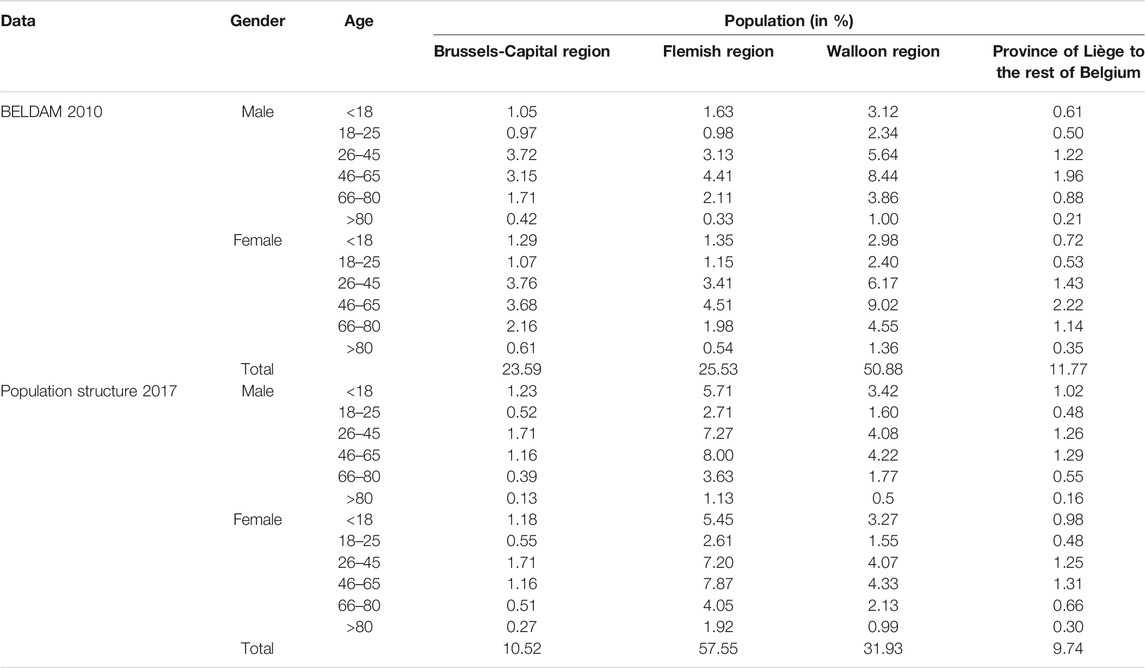
TABLE 2. Comparison of the Belgian population distribution between household travel survey and STATBEL population structure.

Last, the mobile phone data of the province of Liège are provided by Wallonia SPW Mobilité et Infrastructures as aggregated OD matrices. The given data include two collection periods: one is for “working days” from January 15, 2018 to February 08, 2018, and the other is for the carnival and Easter holiday from February 23, 2018 to March 18, 2018. The CDR data have been collected and produced by the telecom company Proximus. The union of polygons representing the cellular coverage in the province of Liège has been built as a Voronoi diagram. However, due to privacy legislation, only aggregated OD matrices are available for this research, without any information about the individuals realizing the underlying trips. The whole province of Liège has been divided into 310 cells by SPW based on the municipalities’ population density. The cells’ origin or destination coordinates are given at a finer level than the municipality (NSI5). It is worth mentioning that STATBEL provides the population distribution at the level of statistical sectors. Based on the data, we can define study zones according to Belgium’s NSI codes of municipalities and administrative districts, such as the municipality (NSI5), the next level (NSI6), and the statistical sectors. We find out that 360 NSI6-zones can be aggregated from STATBEL statistical sectors in the province of Liège. However, it is hard to compare them with 310 mobile phone cells even though most of them (270) have the same NSI6 codes, especially for the Liège district which has a higher population density. Considering the national population structure is defined by Age × Gender × Municipality, we spatially aggregate the 310 cells back to the municipality level to make a comparable visualization with 84 municipalities from STATBEL (Figure 1). Each aggregated mobile phone cell can find the main match with a municipality but may spatially intersect more than one polygon of the city in the province of Liège. To check how closely they match, we calculate the spatial intersection ratios between pairs from two datasets. It shows that the maximum intersection ratio occurs between the zone pair with the same municipality code in two datasets. A boxplot (Figure 2) depicts that around 75% of zone pairs have at least 70% spatial match. There is only one zone pair of mobile phone data and STATBEL which is an outlier, having less than 50% spatial intersection.

FIGURE 1

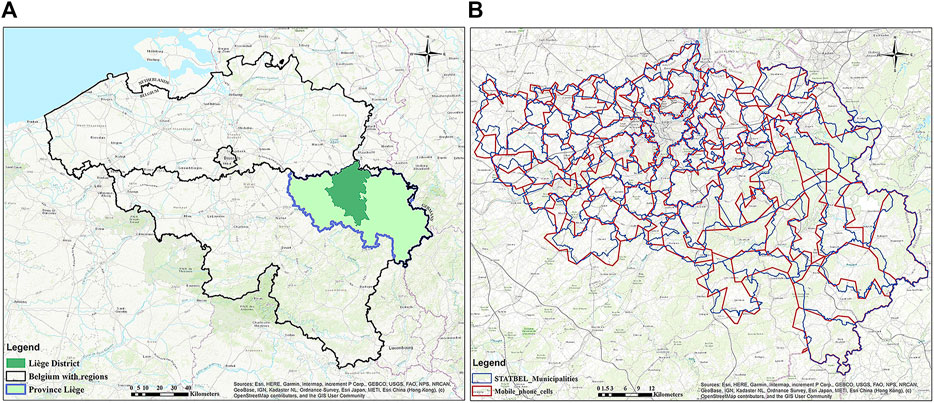
FIGURE 1. (A) Location of the province of Liège in Belgium. (B) Mobile phone cells compared with STATBEL zones at the municipality level.

FIGURE 2

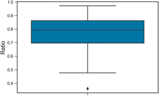
FIGURE 2. Distribution of maximum intersection ratio between mobile phone cells and STATBEL municipalities.

As the trip length distribution is chosen as the validation measure for the simulation framework, the details of Belgian HTS trip lengths and mobile phone–based OD lengths will be described as follows:

1) Trips reported in the Belgian HTS have the respondents’ self-reported travel distance with the known departure and arrival locations. As mentioned in Table 1, the travel survey’s trip locations are measured at the household’s postal code level of details. In comparison, the mobile phone–based trip’s origin and destination locations have been calibrated based on the antenna’s location and the population density. It is unclear how the mobile phone data have been calibrated. However, we find out that at least 80% of the 310 cells’ given coordinates are less than 1,000 m (Euclidean distance) away from the cells’ centroids or less than 250 m (Euclidean distance) away from the STATBEL Liège province NSI6-zone centroids. The mean distance between this 80% of the cells’ origins/destinations and the STATBEL NSI6 centroids is about 13 m, with a standard deviation of 23 m. The remaining 20% of the cells are mainly in the Liège district. Their origin/destination coordinates are distant from the cells’ centroids—meanly 1,551 m with a standard deviation of 561 m—and they cannot be matched with STATBEL NSI6-zones.

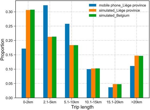
2) We apply Dijkstra’s shortest path algorithm to calculate the OD lengths to have the first impression of trip length distributions in mobile phone data. The interzonal trip length is computed based on the known origin and destination coordinates and the OpenStreetMap network. The intrazonal trip length is set as the mobile phone cell’s radius which is calculated from the cell’s geodesic area. This study uses origin-based (departure locations in the province of Liège) daily mean trips collected in the first period (Table 1) to derive the mobile phone trip lengths. The trips that depart from the Liège province but arrive at places outside of the province will be kept as well. The Belgian HTS trip lengths are self-reported by the respondents and can be directly categorized. We divide trip lengths into the same 6 categories for both data sources. Figure 3 compares the length distributions of approximately two million mobile phone trips with those of around three thousand HTS trips that depart from the Liège province. At the same time, we add the whole of the Belgian HTS trip length distributions to Figure 3. It illustrates the spatial transferability of HTS trips between the province of Liège and Belgium, which confirms the feasibility of using trip length distributions as a validation measure for our modeling framework (Yasmin et al., 2017). However, the categories of trip lengths less than 10 km shown by mobile phone data vary from those shown by the survey data.

3) To show the trip length distributions of the two data sources at a comparable geographical scale, we build the OD matrices at the municipality level for mobile phone data and HTS in the province of Liège. The mean trip length is calculated based on the number of trips between municipalities and the original trip’s length derived in Sub-Section 2. Figure 4 demonstrates that selected municipalities’ sizes decrease the number of short trips shorter than 2 km. However, the difference between the two datasets’ trip length distributions has been reduced compared with that in Figure 3. Besides, Figure 4 indicates the uncertainty of mobile phone–based intrazonal trip lengths calculated by the radius of the cell area. Based on these two figures, we can summarize that BELDAM trip length distributions fit well with those of mobile phone data at the municipality level. However, it is unreliable to compare observed trips shorter than 2 km as mobile phone data have about 50% intrazonal trips, whereas the estimated radiuses as mean trip lengths for mobile phone cells (where intrazonal trips exist) are approximately 30% longer than 2 km. BELDAM trips in the province of Liège also have approximately 50% intrazonal trips. As the trips shorter than 2 km take up more than 25% of the travel survey and a good fit of length distributions with six categories is still found at the municipality level, we decide to keep the category of trips shorter than 2 km during the trip modeling.

FIGURE 3

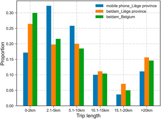
FIGURE 3. Trip length distributions of mobile phone data and Belgian HTS calculated at the level of the recorded data spatial resolution.

FIGURE 4

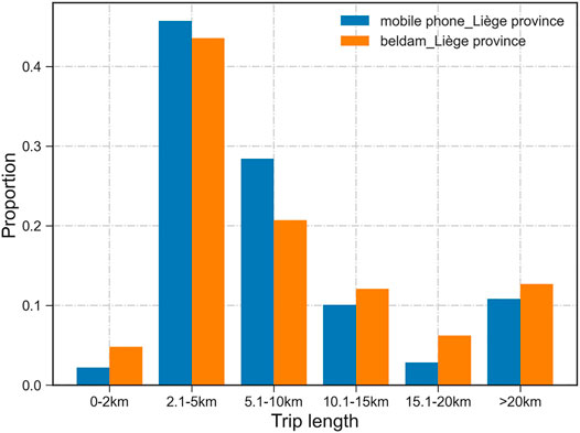
FIGURE 4. Trip length distributions of mobile phone data and Belgian HTS aggregated at the municipality level.

Methods

Modeling Framework

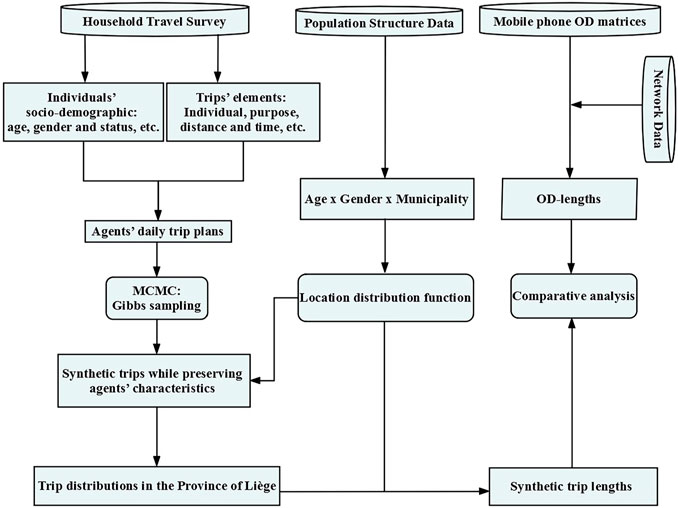
The proposed modeling framework (Figure 5) consists of three components:

 1) A Markov chain Monte Carlo (MCMC) model estimates a representative synthetic population while preserving travel behavior’s heterogeneity. The objective is to set up a full synthetic population with a detailed list of daily activities characterized by sociodemographic attributes and corresponding travel choice sets.

2) Besides the trip length distribution of HTS that has been discussed in the Data section, the reliability of the travel survey is confirmed by comparison with STATBEL population structure concerning age, gender, and residential location distributions.

3) Trip length distributions derived from the mobile phone–based OD matrices are applied to validate the predicted travel distances.

FIGURE 5

FIGURE 5. Proposed overall modeling framework.

To estimate a representative population with a higher level of heterogeneity, MCMC needs conditional probabilities with as many variables involved as possible and as few sampling zeros existing as possible, as it infers the posterior multivariate joint distribution by sequentially drawing random samples from the conditionals. Suppose only individuals and trips in the Liège province of HTS (BELDAM) are used as input. In that case, it will be challenging to infer a joint distribution, as the number of combinations with a nonzero count is low. In this study, we are interested in nine variables concerning an individual’s sociodemographics (i.e., age, gender, and socio-professional status) and the corresponding trip’s elements (i.e., trip motivation, start time, travel duration, travel distance, mode choice, and activity duration). With nine variables of interest or more, the Gibbs sampler can overfit the Liège province’s traditional survey data due to the limited number of observations.

To reduce the sampling zeros, we use the whole of the Belgian HTS as input to the Gibbs sampler, as BELDAM describes the full population. The MCMC-based simulation is deployed using the nine variables mentioned above as input to predict the population and the corresponding trips. After that, instead of directly synthesizing the location variable, trip distributions in the province of Liège are postprocessed based on STATBEL population structure. On the one hand, the population structure deviation is found everywhere from HTS data to the ground truth data (Table 2); on the other hand, Belgium has ten provinces plus Brussels and 581 municipalities, which worsens the sampling performance due to the curse of the dimensionality (Saadi et al., 2016a). Finally, the predicted trip length distributions are compared with the mobile phone–based OD length distributions instead of those stemming from the survey data, which results in a stronger validation approach.

Gibbs Sampling for the Synthesis

This study assumes a population (sociodemographics) with travel choices as the set of attributes $X=\left(x_1, x_2,x_3,\dots ,x_d\right)$. We draw the full joint distribution ${\pi }_X$ and conditional distributions ${\pi }_X\left(x_i|x_{-i}\right)$ directly from the travel survey. Gibbs sampling is used to generate samples using full conditional probability distributions. Three sociodemographic and six travel behavior elements are included as input for the Gibbs sampler. To check the model performance, we implement k-fold cross-validation to define the training and test datasets and ensure that the model is robust enough. The basic concept is to divide the whole dataset into a big training set and a test set; then, the training set is split into smaller k nonoverlapping groups. The sampler is trained using k-1 of the folds as the subtraining data, and the resulting model is validated on the remaining part of the training data. This approach can avoid missing out on some interesting information and reduce bias. The primary test data give the final evaluation. The performance measure reported by k-fold cross-validation is the average of the values computed in the k loops. We keep the samples drawn after the burn-in period to have stable model outcomes and appropriate predicted values. The Gibbs sampling algorithm is structured as follows:

Algorithm 1: Gibbs Sampling

for t←2 to n do

Initialize. ${\mathit{X}}^{\mathit{t-1}}\mathit{=}\left({\mathit{x}}_{\mathit{1}}\mathit{, }{\mathit{x}}_{\mathit{2}}\mathit{,}{\mathit{x}}_{\mathit{3}}\mathit{,}{\mathit{x}}_{\mathit{4}}\mathit{,\dots ,}{\mathit{x}}_{\mathit{d}}\right)$

  for i←1 to d do

   ${\mathit{x}}_{\mathit{1}}^{\mathit{t}}\mathit{\sim \pi }\left({\mathit{x}}_{\mathit{1}}\mathit{|}{\mathit{x}}_{\mathit{2}}^{\mathit{t-1}}\mathit{,}{\mathit{x}}_{\mathit{3}}^{\mathit{t-1}}\mathit{,}{\mathit{x}}_{\mathit{4}}^{\mathit{t-1}}\mathit{,}{\mathit{x}}_{\mathit{5}}^{\mathit{t-1}}\mathit{,\dots ,}{\mathit{x}}_{\mathit{d}}^{\mathit{t-1}}\right)$

   ${\mathit{x}}_{\mathit{2}}^{\mathit{t}}\mathit{\sim \pi }\left({\mathit{x}}_{\mathit{2}}\mathit{|}{\mathit{x}}_{\mathit{1}}^{\mathit{t}}\mathit{,}{\mathit{x}}_{\mathit{3}}^{\mathit{t-1}}\mathit{,}{\mathit{x}}_{\mathit{4}}^{\mathit{t-1}}\mathit{,}{\mathit{x}}_{\mathit{5}}^{\mathit{t-1}}\mathit{,\dots ,}{\mathit{x}}_{\mathit{d}}^{\mathit{t-1}}\right)$

   ${\mathit{x}}_{\mathit{3}}^{\mathit{t}}\mathit{\sim \pi }\left({\mathit{x}}_{\mathit{3}}\mathit{|}{\mathit{x}}_{\mathit{1}}^{\mathit{t}}\mathit{,}{\mathit{x}}_{\mathit{2}}^{\mathit{t}}\mathit{,}{\mathit{x}}_{\mathit{4}}^{\mathit{t-1}}\mathit{,}{\mathit{x}}_{\mathit{5}}^{\mathit{t-1}}\mathit{,\dots ,}{\mathit{x}}_{\mathit{d}}^{\mathit{t-1}}\right)$

   …

   ${\mathit{x}}_{\mathit{i}}^{\mathit{t}}\mathit{\sim \pi }\left({\mathit{x}}_{\mathit{i}}\mathit{|}{\mathit{x}}_{\mathit{1}}^{\mathit{t}}\mathit{,}{\mathit{x}}_{\mathit{2}}^{\mathit{t}}\mathit{,}{\mathit{x}}_{\mathit{3}}^{\mathit{t}}\mathit{,\dots }{\mathit{x}}_{\mathit{i-1}}^{\mathit{t}}\mathit{,\dots ,}{\mathit{x}}_{\mathit{d}}^{\mathit{t-1}}\right)$

 end

 update ${\mathit{X}}^{\mathit{t}}\mathit{=}\left({\mathit{x}}_{\mathit{1}}^{\mathit{t}}\mathit{,}{\mathit{x}}_{\mathit{2}}^{\mathit{t}}\mathit{,}{\mathit{x}}_{\mathit{3}}^{\mathit{t}}\mathit{,}{\mathit{x}}_{\mathit{4}}^{\mathit{t}}\mathit{,\dots ,}{\mathit{x}}_{\mathit{d}}^{\mathit{t}}\right)$

end

Trip Distributions in the Province of Liège

In the HTS data, not all the households are covered from our target province. For instance, two municipalities are found to be missing data when we try to build the OD matrices for the survey data described in the Data section. Therefore, to estimate the agents with trips for the municipalities that are not covered by the surveys, STATBEL population structure data are used. We distribute trips based on the estimated trips’ preserved agent characteristics (i.e., age and gender) while keeping the agent’s travel choice sets (e.g., trip motivation and travel distance). The probability functions draw samples of agents with the corresponding trips for each municipality in Belgium. As a result, we have the distributed trips for the province of Liège that can be further compared with mobile phone data.

Results

Synthetic Population and Daily Trips

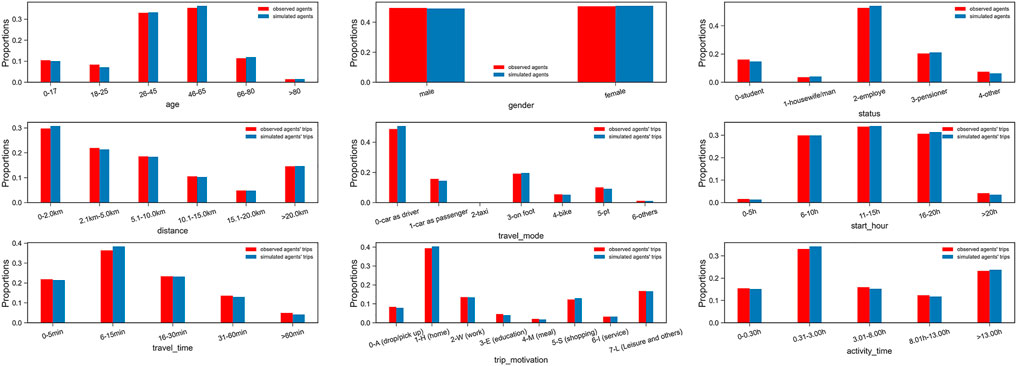
In this experiment, we choose 30% of the HTS data as the final validation set. The k-fold cross-validator is applied to split the training dataset into five folds randomly. Since we are interested in the trip length distributions concerning the full travel plans in this study, it will save time to avoid generating the population’s size to be the same as in the national registered data. We simulate approximately 10% of the population in Belgium. The number of trips is about three times that of the population, according to BELDAM. The standardized root mean squared error (SRMSE) and the coefficient of determination R² metrics are computed to show the quality of estimated joint distributions reported by 5-fold cross-validation. As we have explained in Sub-Section 3.2, there are different training and testing datasets in each fold of the cross-validation procedure, which provides a more reliable assessment of the modeling results. Since this study focuses on the trip length distribution, we first look at the validation results of the partial joint distribution (Age × Gender × Status × Trip_motivation × Distance). Figure 6 illustrates the mean validation score of the 5 folds’ training performance (A) and the final validation result given by 30% of the HTS data (B). The validation quality is improved for the final training result from the 5-fold cross-validator. Table 3 shows that the Gibbs sampler can predict sociodemographics and transport-related attributes with an error, that is, SRMSE = 0.373 and less than 6% variation in the population and their trips’ reproduction for five attributes. However, the R² score significantly decreases with nine variable dimensions, demonstrating that it is unreliable to compare the full joint distribution due to the data sparsity (Garrido et al., 2020). Last, Figure 7 presents the marginal distributions of nine variables of interest.

FIGURE 6

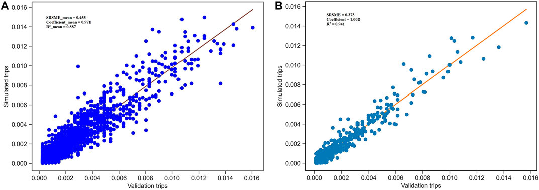
FIGURE 6. (A) Mean validation score of 5 folds’ training performance and (B) the final validation score given by 30% of the HTS data and the total training result from the cross-validator for the partial joint distribution: Age × Gender × Status × Trip motivation × Distance.

TABLE 3

TABLE 3. Partial joint distribution quality for the high-dimensional model.

FIGURE 7

FIGURE 7. Comparison of the marginal distributions of nine attributes.

In Table 2, we see that the Brussels-Capital area has been overrepresented in the travel survey, especially for the age-groups of 26–80 years. In contrast, the Flemish region has been overall underrepresented. The Walloon area has a smaller bias in terms of the observation rate than the other two regions. Instead of considering HTS trip locations as an input variable during the simulation, we distribute the estimated trips based on the trips’ preserved agent characteristics (i.e., age and gender) while keeping the agent’s travel choice sets (e.g., trip motivation and travel distance). The probability functions draw samples of agents with the corresponding trips for each municipality in the province of Liège. As a result, we distribute approximately three hundred thousand trips for the target province. Since the trip length, namely, the travel distance, is one of the nine input variables of the population synthesis, the trip length distributions can be directly generated for the province of Liège. Figure 8 shows that the estimated trip length distributions of the target province have been improved compared with those in Figure 3. Since the simulation in this study has not implemented the trip destination distribution yet, it is still challenging to build an OD matrix for the predicted trips, and a similar comparison with the aggregated OD length shown in Figure 4 cannot be realized here. However, it is still possible to compare the origin-based trip length distribution between two data sources at the municipality level. Next, we extract the number of trips departing from the same origin (municipality) for the estimated and the mobile phone–based trips. Kolmogorov–Smirnov tests (K–S tests) are performed to examine whether the modeled and the observed trip length distributions are drawn from the same distribution.

FIGURE 8

FIGURE 8. Simulated trip length with six categories compared with the mobile phone data.

Validation of the Sampling Model Using Mobile Phone Data

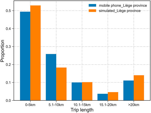
The calibrated and aggregated mobile phone data provide critical information, such as daily mean OD flows, hourly mean OD flows, spatial coordinates of origin and destination, and the hourly interpolated population. This study focuses on the average trip length comparison between the observed and simulated trips. However, mobile phone data can provide the trips generated from the province of Liège, and the trips that involved departure outside eventually arrive at the province of Liège. The simulation requires more details to define a trip that leaves outside a given area and finally arrives at the area of interest. In addition, the HTS data provide only one-day trip plans for each respondent, which makes it challenging to construct multi-day trip plans. This study applies the origin-based daily mean OD flows of mobile phone data and a true network to compute the target study area’s trip lengths. Trips generated from the same origin are extracted to compute each municipality’s trip length distributions. K–S tests are performed to compare two trip length distributions (six categories) of each municipality. The p-values vary from 0.3571 to 0.9999, indicating a similar distribution for each municipality between the modeled and the mobile phone–based observed trip lengths. When we look at Figure 8, it reminds us that uncertainty possibly exists in mobile phone data and HTS, especially for short trips. To double-check the sensibility of validation using trip lengths derived from mobile phone data, we model the trip length with five classes (0–5, 5.1–10, 10.1–15, 15.1–20, and longer than 20 km), which indicates the same distribution trend as well (Figure 9). The predicted trips stemming from the travel survey present more long-distance trips (>15 km). Nevertheless, the proposed simulation framework shows an ability to predict the trip lengths which is close enough to the one measured by the mobile phone data.

FIGURE 9

FIGURE 9. Simulated trip length with five categories compared with the mobile phone data.

Discussion and Conclusion

Despite the advancement of the activity-based model, the lack of reliable data is often a critical problem that researchers encounter. To meet the challenge, we implement experiments using multiple data sources and examine modeling results both internally and externally. This study looks deep into the currently available mobility data in the province of Liège, Belgium. It shows the deviation of the surveyed data from the national register of citizens and the possible contribution of the second data type to the modeling of travel demand. As an essential part of modeling for practical applications in the real-world context, validation using various data sources can contribute to the modeling framework in different ways. This study demonstrates the potential advantage of a new big data source for agent-based models, which are in general estimated based on conventional travel surveys. Mobile phone data offer stronger validation measures for the travel simulation framework concerning the higher population penetration rates than traditional surveys. This is in line with Liu et al. (2014), who concluded that measures can be developed from mobile phone data and used to validate the existing activity-based simulation models. Also, we apply k-fold cross-validation to estimate the actual travel demand’s representation, including the simultaneous inference of travelers’ sociodemographics and their behavior choice sets. One of the limitations is that all variables of interest are treated discretely in the simulation. The choice helps construct the empirical joint distribution of high-dimensional data and quickly finds the population clusters with different daily travel plans. It has provided comparable heterogeneity of travel behaviors with the observed one. However, the more attributes are involved in the population synthesis; the more deviations appear between the joint distributions. Continuous variables are discretized to be easily incorporated in the Gibbs sampler while bringing us another restriction: agents with the same sociodemographics gather automatically into the same clusters, which breaks each agent’s trips’ original temporal and spatial connection. To build a full activity-based schedule, the model requires a new labeling process for individual activity-sequence differentiation. It is also one of the main research priorities to be addressed in the future.

Concerning the aggregated mobile phone data’s lack of user records, we choose the trip length as the variable of interest to validate the simulation framework’s performance. As a first outcome of the validation, we see a close match between the synthesized travel distance and the observed OD length. However, long-distance trips are slightly overestimated. The possible cause can be the inherent uncertainty of both travel surveys and mobile phone data. Also, we show the deviation of the surveyed population distribution from the national population structure data. Calibration parameters can be defined into the location distribution choice based on the comparison results. In the future, we are also interested in taking advantage of other key mobile phone data information, such as the intensity of OD trips and the spatiotemporal variation of the OD flows, in calibrating the simulated trips at more disaggregated spatiotemporal scales.

Data Availability Statement

The original contributions presented in the study are included in the article. Further inquiries can be directed to the corresponding author.

Author Contributions

Conceptualization and methodology: SG, IS, and MC; investigation, software, validation, and formal analysis: SG; data collection: SG and JT; writing—original draft preparation: SG; writing—review and editing: SG, IS, JT, and MC; supervision: MC; project administration: SG. All authors have read and agreed to the published version of the manuscript.

Funding

This work has been funded through the Wal-e-Cities Project, supported by the European Regional Development Fund (ERDF) and the Walloon Region and through the Special Fund for Research for Project No. 11473, financed by the French Community of Belgium (Wallonia-Brussels Federation).

Conflict of Interest

The authors declare that the research was conducted in the absence of any commercial or financial relationships that could be construed as a potential conflict of interest.

Acknowledgments

We would like to thank Wallonia SPW Mobilité et Infrastructures for kindly providing the mobile phone data.

Appendix A

A1. cross-classification of the variables of interest with respect to the trip purpose (in %)

References

Anda, C., Erath, A., and Fourie, P. J. (2017). Transport Modelling in the Age of Big Data. Int. J. Urban Sci. 21, 19–42. doi:10.1080/12265934.2017.1281150

CrossRef Full Text | Google Scholar

Arentze, T. A., and Timmermans, H. J. P. (2004). A Learning-Based Transportation Oriented Simulation System. Transportation Res. B: Methodological 38 (7), 613–633. doi:10.1016/j.trb.2002.10.001

CrossRef Full Text | Google Scholar

Axhausen, K. W. (2007). “Concepts of Travel Behaviour Research,” in Threats from Car Traffic to the Quality of Urban Life (Emerald Group Publishing Limited).

Google Scholar

Bassolas, A., Ramasco, J. J., Herranz, R., and Cantú-Ros, O. G. (2019). Mobile Phone Records to Feed Activity-Based Travel Demand Models: MATSim for Studying a Cordon Toll Policy in Barcelona. Transportation Res. A: Pol. Pract. 121 (3), 56–74. doi:10.1016/j.tra.2018.12.024

CrossRef Full Text | Google Scholar

Bazzan, A. L. C., and Klügl, F. (2014). A Review on Agent-Based Technology for Traffic and Transportation. Knowledge Eng. Rev. 29 (3), 375–403. doi:10.1017/S0269888913000118

CrossRef Full Text | Google Scholar

Borysov, S. S., Rich, J., and Pereira, F. C. (2019). How to Generate Micro-agents? A Deep Generative Modeling Approach to Population Synthesis. Transportation Res. C: Emerging Tech. 106 (8), 73–97. doi:10.1016/j.trc.2019.07.006

CrossRef Full Text | Google Scholar

Farooq, B., Bierlaire, M., Hurtubia, R., and Flötteröd, G. (2013). Simulation Based Population Synthesis. Transportation Res. Part B: Methodological 58 (12), 243–263. doi:10.1016/j.trb.2013.09.012

CrossRef Full Text | Google Scholar

Franco, P., Johnston, R., and McCormick, E. (2020). Demand Responsive Transport: Generation of Activity Patterns from Mobile Phone Network Data to Support the Operation of New Mobility Services. Transportation Res. Part A: Pol. Pract. 131 (1), 244–266. doi:10.1016/j.tra.2019.09.038

CrossRef Full Text | Google Scholar

Garrido, S., Borysov, S. S., Pereira, F. C., and Rich, J. (2020). Prediction of Rare Feature Combinations in Population Synthesis: Application of Deep Generative Modelling. Transportation Res. Part C: Emerging Tech. 120 (9), 102787. doi:10.1016/j.trc.2020.102787

CrossRef Full Text | Google Scholar

González, M. C., Hidalgo, C. A., and Barabási, A.-L. (2008). Understanding Individual Human Mobility Patterns. Nature 453, 779–782. doi:10.1038/nature06958

PubMed Abstract | CrossRef Full Text | Google Scholar

Goulding, J. (2018). Best Practices and Methodology for OD Matrix Creation from CDR Data. (Nottingham: NLAB, University of Nottingham).

Habib, K. N. (2018). A Comprehensive Utility-Based System of Activity-Travel Scheduling Options Modelling (CUSTOM) for Worker’s Daily Activity Scheduling Processes. Transportmetrica A: Transport Sci. 14 (4), 292–315. doi:10.1080/23249935.2017.1385656

CrossRef Full Text | Google Scholar

Hörl, S., and Balac, M. (2020). Reproducible Scenarios for Agent-Based Transport Simulation: A Case Study for Paris and Île-De-France. (Zurich: IVT, ETH Zurich).

Iqbal, M. S., Choudhury, C. F., Wang, P., and González, M. C. (2014). Development of Origin-Destination Matrices Using Mobile Phone Call Data. Transportation Res. Part C: Emerging Tech. 40, 63–74. doi:10.1016/j.trc.2014.01.002

CrossRef Full Text | Google Scholar

Kang, Y., Gao, S., Liang, Y., Li, M., Rao, J., and Kruse, J. (2020). Multiscale Dynamic Human Mobility Flow Dataset in the U.S. During the COVID-19 Epidemic. Sci. Data 7 (1). doi:10.1038/s41597-020-00734-5

PubMed Abstract | CrossRef Full Text | Google Scholar

Kraemer, M. U. G., Sadilek, A., Zhang, Q., Marchal, N. A., Tuli, G., Cohn, E. L., et al. (2020). Mapping Global Variation in Human Mobility. Nat. Hum. Behav. 4 (8), 800–810. doi:10.1038/s41562-020-0875-0

PubMed Abstract | CrossRef Full Text | Google Scholar

Li, T., Sun, D., Jing, P., and Yang, K. (2018). Smart Card Data Mining of Public Transport Destination: A Literature Review. Information 9 (1), 18. doi:10.3390/info9010018

CrossRef Full Text | Google Scholar

Liu, F., Janssens, D., Cui, J., Wang, Y., Wets, G., and Cools, M. (2014). Building a Validation Measure for Activity-Based Transportation Models Based on Mobile Phone Data. Expert Syst. Appl. 41 (14), 6174–6189. doi:10.1016/j.eswa.2014.03.054

CrossRef Full Text | Google Scholar

Liu, F., Janssens, D., Cui, J., Wets, G., and Cools, M. (2015). Characterizing Activity Sequences Using Profile Hidden Markov Models. Expert Syst. Appl. 42 (13), 5705–5722. doi:10.1016/j.eswa.2015.02.057

CrossRef Full Text | Google Scholar

Medina, S., and Erath, A. (2013). Estimating Dynamic Workplace Capacities by Means of Public Transport Smart Card Data and Household Travel Survey in Singapore. Transportation Res. Rec. 2344 (-1), 20–30. doi:10.3141/2344-03

CrossRef Full Text | Google Scholar

Ramadan, O. E., and Sisiopiku, V. P. (2019). “A Critical Review on Population Synthesis for Activity- and Agent-Based Transportation Models,” in Transportation Systems Analysis and Assessment (London: IntechOpen). doi:10.5772/intechopen.86307

CrossRef Full Text | Google Scholar

Rojas, M. B., Sadeghvaziri, E., and Jin, X. (2016). Comprehensive Review of Travel Behavior and Mobility Pattern Studies that Used Mobile Phone Data. Transportation Res. Rec. 2563 (10), 71–79. doi:10.3141/2563-11

CrossRef Full Text | Google Scholar

Roorda, M. J., Miller, E. J., and Habib, K. M. N. (2008). Validation of TASHA: A 24-h Activity Scheduling Microsimulation Model. Transportation Res. Part A: Pol. Pract. 42 (2), 360–375. doi:10.1016/j.tra.2007.10.004

CrossRef Full Text | Google Scholar

Saadi, I., Mustafa, A., Teller, J., and Cools, M. (2016b). Forecasting Travel Behavior Using Markov Chains-Based Approaches. Transportation Res. Part C: Emerging Tech. 69 (8), 402–417. doi:10.1016/j.trc.2016.06.020

CrossRef Full Text | Google Scholar

Saadi, I., Mustafa, A., Teller, J., Farooq, B., and Cools, M. (2016a). Hidden Markov Model-Based Population Synthesis. Transportation Res. Part B: Methodological 90 (8), 1–21. doi:10.1016/j.trb.2016.04.007

CrossRef Full Text | Google Scholar

Sun, L., and Erath, A. (2015). A Bayesian Network Approach for Population Synthesis. Transportation Res. Part C: Emerging Tech. 61, 49–62. doi:10.1016/j.trc.2015.10.010

CrossRef Full Text | Google Scholar

Wang, Z., He, S. Y., and Leung, Y. (2018). Applying Mobile Phone Data to Travel Behaviour Research: A Literature Review. Trav. Behav. Soc. 11 (3), 141–155. doi:10.1016/j.tbs.2017.02.005

CrossRef Full Text | Google Scholar

Yan, X.-Y., Wang, W.-X., Gao, Z.-Y., and Lai, Y.-C. (2017). Universal Model of Individual and Population Mobility on Diverse Spatial Scales. Nat. Commun. 8 (1), 1–9. doi:10.1038/s41467-017-01892-8

PubMed Abstract | CrossRef Full Text | Google Scholar

Yasmin, F., Morency, C., and Roorda, M. J. (2017). Macro-, Meso-, and Micro-level Validation of an Activity-Based Travel Demand Model. Transportmetrica A: Transport Sci. 13 (3), 222–249. doi:10.1080/23249935.2016.1249437

CrossRef Full Text | Google Scholar

Zhu, Y., and Ferreira, J. (2014). Synthetic Population Generation at Disaggregated Spatial Scales for Land Use and Transportation Microsimulation. Transportation Res. Rec. 2429, 168–177. doi:10.3141/2429-18

CrossRef Full Text | Google Scholar

Zilske, M., and Nagel, K. (2015). A Simulation-Based Approach for Constructing All-Day Travel Chains from Mobile Phone Data. Proced. Comp. Sci. 52 (1), 468–475. doi:10.1016/j.procs.2015.05.017

CrossRef Full Text | Google Scholar