Assignment Matrix Free Algorithms for On-line Estimation of Dynamic Origin-Destination Matrices

Dynamic Traffic Assignment (DTA) models represent fundamental tools to forecast traffic flows on road networks, assessing the effects of traffic management and transport policies. As biased models lead to incorrect predictions, which can cause inaccurate evaluations and huge social costs, the calibration of DTA models is an established and active research field. When it comes to estimating Origin-Destination (OD) demand flows, perhaps the most important input for DTA models, one algorithm suggested to outperform all the others for real-time applications: the Kalman Filter (KF). This paper introduces a non-linear Kalman Filter framework for online dynamic OD estimation that reduces the number of variables and can easily incorporate heterogeneous data sources to better explain the non-linear relationship between traffic data and time-dependent OD-flows. Specifically, we propose a model that takes advantage of Principal Component Analysis (PCA) to capture spatial correlations between variables and better exploit the local nature of a specific KF recently proposed in literature, the Local Ensemble Transformed Kalman filter (LETKF). The main advantage of the LETKF is that the Kalman gain is not explicitly formulated which means that, differently from other approaches proposed in the literature, there is no need to compute the assignment matrix or its approximation. The paper shows that the LETKF can easily incorporate different data sources, such as traffic counts and link speeds. Additionally, thanks to the PCA, the model can identify local patterns within the data and better explain the correlation between variables and data. The effectiveness of the proposed methodology is demonstrated first through synthetic experiments where non-linear functions are used to benchmark the model in different conditions and then on the real-world network of Vitoria, Spain (2,884 nodes, 5,799 links) using the mesoscopic simulator Aimsun. Results show that the proposed method leads to better state estimation performances with respect to other Ensemble-based Kalman filters, providing improvements as high as 64% in terms of traffic data reproduction with a 17-fold problem dimensionality reduction.

Introduction

Due to the rapid growth of road traffic, all major cities of the world are facing severe congestion problems. It is clear that simply increasing the infrastructure supply is not physically or economically feasible. The ever-growing pressure of travel demand on existing transport facilities generates significant societal, environmental and economic losses, due to the increase of pollutant emissions and travel times. To tackle this issue, practitioners and researchers in the transportation field rely on traffic simulation models to evaluate and implement efficient measures, ranging from off-line planning to real-time traffic management solutions. However, the efficiency of these tools depends on their ability to correctly predict traffic conditions.

Travel demand is arguably the most important input for traffic simulation models, as both the planning and management of traffic solutions require good knowledge of current and forecasted demand. In dynamic models, demand is usually discretized in the form of Origin-Destination (OD) matrices, where each cell represents all trips from an origin zone to a destination zone started during a specific time interval. A widely adopted procedure uses traffic counts to estimate these matrices, seeking the best possible approximation of OD flows that minimizes the error between simulated and available traffic data. The relation between OD matrices and traffic counts is generally expressed through assignment matrices, which are hard to obtain and impose a simple linear relationship between link and demand flows (Frederix et al., 2013). Traditionally, this procedure can be applied off-line (for medium to long term planning) or on-line (for real-time traffic prediction). The Dynamic OD demand Estimation problem leads to two different approaches: simultaneous or sequential (Cascetta et al., 1993; Cantelmo and Viti, 2020). In the latter approach, matrices are individually estimated, from the first-time interval to the last one, while keeping the matrices calculated in the previous intervals fixed. By pursuing a sequential approach, the computational complexity of the problem decreases as the problem itself can be split into a set of simpler sub-problems and every estimated matrix can be used as the starting estimate for the next time interval. Thus, the sequential approach is a must for online applications, where computational times are an important constraint in the estimation process.

One algorithm that has been proven to outperform all the others for the Online Dynamic Demand Estimation (ODDE) problem is the Kalman Filter (Chang and Wu, 1994; Van der Zijpp and Hammerslag, 1994; Ashok, 1996; Zhou and Mahmassani, 2007). The Kalman Filter uses a series of measures obtained over time to estimate the most likely status of an unknown variable. In the case of on-line estimation of demand, time-dependent OD flows are the unknown variables and observed traffic conditions are the data. However, despite more than 20 years of intense research efforts, the ODDE has not yet been solved in such an effective way to be applied for real problems. Based on the literature, we can distinguish between three main sources of complexity in ODDE:

1. Number of variables: the ODDE procedure generally returns effective results when the number of observations (traffic data) is similar to the number of unknowns (OD flows). However, as this usually does not occur in practice, dimensionality reduction techniques should be deployed to avoid this issue (Marzano et al., 2009; Djukic et al., 2012; Xia et al., 2018).

2. Non-linear relationships between variables: there are two main ways of considering non-linearity within the ODDE, which ideally should be jointly considered. One way is to include different data sources in order to increase the observability of the system. For instance, jointly considering speeds, densities and counts can help to better understand traffic phenomena (Balakrishna et al., 2007; Frederix et al., 2011; Yang et al., 2017). Secondly, describing non-linear systems entails deploying non-linear models. The conventional Kalman Filter is a simple linear model, thus several non-linear extensions have been proposed (Antoniou et al., 2007).

3. Demand structure: mobility demand derives from the demand for activities, and thus, it has a structure. Different models should be used to target different components of the demand, including random fluctuations, structural, and seasonal trends, as well as regular trends (Zhou and Mahmassani, 2007; Cantelmo et al., 2019; Behara et al., 2020).

This paper introduces a non-linear Kalman Filter framework for ODDE, that considers the three sources of complexity previously reported. Through the adoption of Principal Component Analysis (Jolliffe, 2002)(Jolliffe, 2002), it works on exploiting the demand structure and on reducing the number of variables. It is assignment matrices-free, which means that it can easily incorporate heterogeneous data sources to better explain the non-linear relationship between traffic data and time-dependent OD-flows.

The remainder of the paper is structured as follows. Section Literature Review provides a brief literature review of the ODDE problem solved through the Kalman filter and its non-linear extensions. The model, an extension of the Local Transformed Ensemble Kalman Filter (LTEKF) proposed in Carrese et al. (2017) is then presented in section The Model: PCA-Local Transformed Ensemble Kalman Filter. Section Applications and Results shows the numerical results on a synthetic experiment and on the real-world network of the city of Vitoria, Spain. Lastly, section Conclusions provides some concluding statements and remarks.

Literature Review

Online Dynamic Demand Estimation

Travel demand refers to the entirety of trips between all the traffic zones of a transport network, taking into account the different travel purposes, time frames and modes of transport (Cascetta, 1984). From a modeling perspective, travel demand consists mainly of an origin-destination (OD) matrix with each cell representing all trips from an origin zone O to a destination zone D.

In the dynamic case, the temporal OD demand is usually represented by a sequence of matrix “slices” where each demand slice corresponds to a departure time interval. Estimation of temporal OD demand can be performed for both within-day (intra-period) and day-to-day (inter-period) dynamic frameworks, as well as for off-line (medium-long term planning and design) and on-line (real-time management) applications (Cipriani and Nigro, 2017).

In the on-line within-day formulation, OD flows are estimated as a sequence of separated intervals adopting a rolling-horizon approach. This is called sequential approach and it is formulated as follows:

$\begin{array}{ll}{d}^{\ast }{}_{nh}\text{= argmin}[f_1(x_{nh},x^{\ast }{}_{nh})+f_2(t_{nh}(x_{nh}|d^{\ast }{}_1\dots .d^{\ast }{}_{nh}),t^{\ast }{}_{nh})]& (1)\end{array}$

The objective in (1) is to find the matrix d^*_nh for each time interval n_h of the planning horizon T, minimizing: (i) a measure of distance f₁ between the unknown ODs x_nh and some a priori target matrix x^*_nh (seed matrix); (ii) a measure of distance f₂ between simulated traffic data t_nh and traffic measurements t^*_nh.

Simulated traffic data derive by the Dynamic Traffic Assignment (DTA) of the unknown ODs, fixing the ODs of previous time slices. The first component f₁in (1) allows to overcome the non-uniqueness of the solution of the demand estimation problem, where in on-line dynamic formulations, off-line dynamic matrices are usually adopted as the target ones.

Kalman Filter and Non-linear Extensions for ODDE

One of the most established approaches for ODDE is to re-formulate the problem as a state-space model and, successively, to adopt a Kalman Filtering (KF) approach (Okutani and Stephanedes, 1984) to solve it. The state-space model is a useful abstraction for dynamic systems that describes the behavior of said systems through three equations:

1. The transition equations, which capture the evolution of the system over time;

2. The measurement equations, which map the state variables to the observed data;

3. The analysis equation, which corrects the estimate derived by the transition equations through the results of the measurements equations and the Kalman gain.

The KF algorithm (Kalman, 1960) (Kalman, 1960)is based on the solution of a least-square cost function in an incremental way, allowing to update the OD flows when new traffic data is available. In order to include the structure of the demand within the estimation framework, Ashok and Ben-Akiva (1993) formulated the KF in terms of deviations between the actual and the historical OD flows.

The KF algorithm represents one of the most widely adopted solution framework for the online OD estimation problem (Barcelo and Montero, 2015; Zhang et al., 2017; Marzano et al., 2018; Krishnakumari et al., 2019; Liu et al., 2020). However, its application to the online OD estimation problem has several drawbacks. Firstly, both the transition equation and the measurement equation assume a linear relation between variables. In the case of the transition equation, this relation is usually represented in the form of an autoregressive process (Ashok, 1996), while the assignment matrices are usually used to feed the measurement equation. However, the assignment matrices are then assumed as fixed in the measurement equations to simplify the process and, lastly, standard KF is not able to handle a large number of variables, as it requires intensive linear algebra computations (Bierlaire and Crittin, 2004).

As these formulations poorly represent traffic dynamics, non-linear models need to be deployed in real cases (Antoniou et al., 2007).

This paper will focus on the family of Ensemble Kalman filters (EnKF), introduced by Evensen (2003). EnKF chooses an ensemble of initial conditions around the current estimate and propagates each ensemble member based on a non-linear model. Thus, the uncertainty of the estimation is propagated from one time interval to the next and the ensemble is used to parametrize the distribution of the state variables.

The size of the ensemble has to be chosen so that it is statistically representative of the model (Kalnay, 2002) and must span the model sub-space adequately (Oke et al., 2007) or the system may be undersampled and thus lead to unwanted errors, such as inbreeding, filter divergence, and spurious correlations (Whitaker and Hamill, 2002; Lorenc, 2003; Furrer and Bengtsson, 2007). Several approaches have been implemented to avoid the problems caused by undersampling, such as covariance inflation (Anderson and Anderson, 1999) and localization (Hamill et al., 2001).

The size of the ensemble also affects the computational time of the EnKF. All the Ensemble-based Kalman filters tend to be computationally expensive as the state variables ensemble must be maintained throughout the entire time horizon. Furthermore, when computing the dependency between OD flows and observed measurements, for each time interval k runs of the DTA model are required, where k is the number of the elements in the ensemble. Since the DTA performance is highly dependent on the number of OD pairs on the network, to obtain a sustainable prediction time for Ensemble-based Kalman filters algorithm, some computational time reduction approaches must be pursued, such as accelerating the solution algorithm of the DTA or reducing the dimensionality of the problem.

An interesting extension of the EnKF is the Local Ensemble Transformed Kalman filter (LETKF) (Hunt et al., 2007), which efficiently deals with non-linear problems, large-scale models and datasets combining the advantages of two ensemble-based filters: the Local Ensemble Kalman filter and the Ensemble Transformed Kalman filter (ETKF) (Bishop et al., 2001; Wang et al., 2004).

The LETKF adds two extension to the basic EnKF. First, it allows to minimize the Kalman filter cost function in the ensemble space, thus reducing the dimension of the problem and the problem complexity (it is “transformed”). Second, it provides a framework for data assimilation that allows a system-dependent localization strategy, breaking down the problem into sub-problems to be solved in a parallel fashion (it is “local”). As in all the EnKFs, the LETKF avoids the linearization of the dependency between OD flows and observed measurements, by implicitly capturing it through a traffic simulator rather than through an analytic formula.

As pointed out in Hunt et al. (2007) and Carrese et al. (2017), the LETKF provides a framework for data assimilation that allows a localization strategy, i.e., cutting off longer range correlations at a specified distance. Generally, it is performed by applying a Schur product with a correlation function with local support, meaning that the function will be dependent on the Euclidean distance between variables and will be non-zero only in a small local region. However, this idea holds true only for the prediction process of selected dynamic systems, such as weather forecasting, where the spatial correlation between variables does depend on the Euclidean distance between them. Since traffic is sprawled everywhere on the network, the same does not hold for traffic dynamic systems, as OD flows are not directly correlated by Euclidean distance. For the ODDE, the “local” approach means dividing the network into subnetworks and the demand matrix into submatrices, each submatrix containing the ODs that mostly affect the traffic measurements in the corresponding subnetwork. This is something that has already been tested for the off-line OD estimation problem (Cantelmo et al., 2014; Antoniou et al., 2015). However, similarly to methods that explicitly use the assignment matrix, this entails developing procedures to explicitly map the relative weight of the information (e.g., how ODs and link flows are correlated).

Contribution Statement

It is well-known that the ODDE is a highly non-linear, highly undetermined, and computationally demanding problem. Based on the analysis of the state of the art, it emerges that there is a clear need for efficient and robust solution methods able to handle large networks and heterogeneous data sources.

LETKF represents a recent development of EnKF for the ODDE problem, as it is suitable for highly non-linear problems and large-scale networks and datasets. So far, the model has been used for small networks only, thus, the “local” peculiarity of LETKF, which has only been mentioned but not implemented in Carrese et al. (2017), remains one of the main and most interesting research lines for the applicability of the model on large-scale world networks. To fill this gap, this paper introduces a methodology that combines the Principal Component Analysis and the LETKF (PCA-LETKF). Differently from the methods proposed in Cantelmo et al. (2014) and Antoniou et al. (2015), the Principal Component Analysis (PCA) allows in fact to capture spatial correlations between variables without the need to explicitly map these relationships. The PCA is a powerful tool for data analysis that aims to identify patterns in high-dimensional datasets and reduce the number of dimensions without much loss of information. This is achieved by transforming the dataset into a new set of variables—the Principal Components (PCs)—which are uncorrelated and ordered so that the first few retain most of the variation present in all of the original variables (Jolliffe, 2002). PCA is an assumption-free procedure that already calculates how ODs are correlated (Prakash et al., 2018; Qurashi et al., 2019). As showed by Djukic et al. (2012) and Prakash et al. (2018), replacing the OD demand with its Principal Components reduces the problem complexity thus making the ODDE problem simpler. This paper shows that the PCA also identifies the variables that are highly correlated and provides a good classification for the localization framework. Thus, by finding the spatial correlation between variables, the PCA empowers the LETKF model to better exploit its “local” nature.

We show that, for transport applications, the proposed PCA-LETKF outperforms conventional EnKF, including the LETKF. The reason is that the PCA finds spatial correlations between variables, which leads to a smaller number of ensembles required, with respect to the conventional EnKF, to achieve better estimates.

The Model: PCA-Local Transformed Ensemble Kalman Filter

The road traffic network is modeled by a directed graph G = {n, l} where n is the set of nodes and l is the set of links. The simulated horizon T is divided in equal time intervals h = 1, …, t.

Creation of the Starting Dataset

According to Prakash et al. (2018), multiple estimates of the OD flows are required to obtain the principal components of an OD flow vector. One reasonable approach would be using an offline calibration procedure to estimate the OD flows over multiple days and compose a m × n_OD data matrix X, where m is the number of estimates used and n_OD is the number of OD pairs in the network. In practice, every x_i estimate is created from the seed matrix x (having dimension n_OD × n_h) as:

$\begin{array}{ll}{x}_i=x\times (1-q_{i}R\Delta )& (2)\end{array}$

where R is a normally distributed random vector with mean 0 and values between 0 and 1, Δ is a ±1 Bernoulli distribution random vector used to randomize the increase or decrease of each estimate x_i. Lastly, q_i is a random coefficient to specify the scale of randomization.

A centered data matrix $\tilde{X}$ is obtained by subtracting the mean $\overline{X}$ from each column of the matrix X, since having a zero mean dataset simplifies the problem.

Generation of the PC Components

A Singular Valued Decomposition (SVD) is performed on the matrix $\tilde{X}$:

$\begin{array}{ll}\tilde{X}=U\sum V^T& (3)\end{array}$

where ∑ is a m × n_OD matrix with positive values called singular values, U is a m × m matrix with orthogonal column vectors called the left singular vectors and V is a n_OD × n_OD matrix with orthogonal column vectors called the right singular vectors.

The column of the matrix V are the principal component directions, which represent the eigenvectors of the sample covariance matrix $\frac{1}{m}{\tilde{X}}^T\tilde{X}$. The first r PC-directions—sorted highest to lowest according to the values of the ∑ vector—that explain more than 95% variance of the data matrix are selected to form the n_OD × r matrix V.

$\begin{array}{ll}V=\left[v_1{v}_2\dots v_{r-1}{v}_r\right]& (4)\end{array}$

where v₁ represents the PC direction with the largest sample variance, v₂ represents the PC direction with the largest sample variance that is orthogonal to v₁ and so on.

Then, the PCs for the time interval h − 1 are generated as:

$\begin{array}{ll}{z}_{h-1}^a=V^T{x}_{h-1}^a& (5)\end{array}$

where $x_{h-1}^a$ are the a priori OD flows (of the seed matrix) containing all the trips departing during the time interval h − 1.

It must be taken into account that the principal components, as computed above, capture the structural spatial relationship between the OD flows and not their temporal relationships. As OD demand can change through the day, it would be desirable to compute several matrices V_h relative to the specific time interval h. But calculating time-interval specific principal components can have high data requirements, hence why the feature vector V is considered constant across intervals, implying that the statistical correlation between OD flows is constant through the chosen time frame. This is considered to be an acceptable approximation when, for example, the estimation time frame corresponds to only the morning hours (i.e., from 7:00 a.m. to 12:00 p.m., as in the case studies discussed in the following sections), whereas, if the entire day demand is considered, issues may arise as the afternoon peak hours may affect the correlation in the morning peak hours and vice versa.

Generation of the a priori Ensemble

Given the a priori PCs $z_{h-1}^a$, an ensemble is generated:

$\begin{array}{ll}{z}_{h-1}=\left\{z_{h-1}^i:i=1\dots k\right\}& (6)\end{array}$

where k is the number of members of the ensemble. In ensemble-based filters, the ensemble can be obtained “offline,” from the last matrices estimated during iterations of an off-line adjustment process or several matrices obtained from off-line adjustment conducted for several days. In this paper, as we are generating an ensemble of PCs, the ensemble is generated by perturbing the a priori PCs $z_{h-1}^a$ through a randomization vector S_i (containing normally distributed values from 0 to the arbitrarily chosen maximum percentage error given to the PCs) and a Bernoulli distributed vector.

$\begin{array}{ll}{z}_{h-1}^i=z_{h-1}^a\times (1-S_i\Delta )& (7)\end{array}$

Transition Equations

From each member of the a priori ensemble $z_{h-1}^i$, the background state estimate for the following time interval h is obtained as:

$\begin{array}{ll}{z}_{h|h-1}^i=F_{h|h-1}{z}_{h-1}^i& (8)\end{array}$

F_h|h−1 is the propagation map, that captures the evolution of the system over time through an autoregressive process, as proposed in Ashok (1996)(Ashok, 1996). Several approaches can be found in literature, with one of them being a polynomial approximation that interpolates each a priori vector by the average of the a priori ensemble from one time interval to the next. Furthermore, as ach ensemble is forecasted into the future time interval independently, this makes this formulation well-suited for parallel processing.

The mean value ${\overline{z}}_{h|h-1}$, the deviation $\Delta Z_{h|h-1}^i$ and the covariance matrix P_h|h−1 are then computed.

$\begin{array}{ll}{P}_{h|h-1}={(k-1)}^{-1}{\displaystyle \sum _{i=1}^k}\left(\Delta Z_{h|h-1}^i\right){\left(\Delta Z_{h|h-1}^i\right)}^T& (9)\end{array}$

And the PCs background ensemble z_h|h−1 is transformed back into OD flows to perform the assignment through a DTA simulator:

$\begin{array}{ll}{x}_{h|h-1}^i=V{z}_{h|h-1}^i& (10)\end{array}$

The formulation (10) is an approximation as we reduced the dimensionality of the PC-directions matrix V. Thus, when reconstructing the data, the dimensions that have been discarded are lost.

Measurement Equations

The state variables until time interval h are mapped onto the simulated measurements y at time h:

$\begin{array}{ll}{y}_h^i=H\left(x_1^i,\dots ,x_{h-1}^i,x_{h|h-1}^i\right)& (11)\end{array}$

$y_h^i$ is a vector that contains all measurements chosen, such as link flows, speeds, etc… H represents the non-linear model that maps the OD flows to the traffic measurements. It is not required for H to have an analytic formulation as in the LETKF algorithm the Kalman gain is not explicitly formulated. For the linear Kalman filter and other ensemble based Kalman filters, H consisted of the assignment matrix, whereas for the LETKF model H is considered a “black box” that contains a DTA procedure used to simulate the traffic measurements that will be the outputs of the measurement equations (11).

Then, the mean ${\overline{y}}_h$ and deviation ΔY_h are computed. The covariance matrix of the measurements R is usually assumed constant across time intervals.

Coordinate Change

A coordinate change from the PCs space (r dimension space) to the ensemble space (k dimension space) takes place. The covariance matrix for the analysis state in the k-dimension space becomes:

$\begin{array}{ll}\widetilde{P_h}={\left[(k-1)I+{(\Delta Y_h)}^T{R}^{-1}\Delta Y_h\right]}^{-1}& (12)\end{array}$

where I is the identity matrix (k × k dimension). The average of the analysis state in the k-dimension space is:

$\begin{array}{ll}{\overline{w}}_h=\widetilde{P_h}{(\Delta Y_h)}^T{R}^{-1}(y_h^0-{\overline{y}}_h)& (13)\end{array}$

where $y_h^0$ are the observed traffic counts for the time interval h and $\widetilde{P_h}{(\Delta Y_h)}^T{R}^{-1}$ represents the Kalman gain. This transformation allows dealing with a Kalman gain that is not function of either H or its Jacobian, which is usually required in other KF approaches.

Return to the PCs Space

The background PCs ensemble ${\overline{z}}_{h|h-1}$ is corrected and the a priori ensemble for the next time interval z_h and its covariance matrix P_h are obtained as:

$\begin{array}{ll}{\overline{z}}_h={\overline{z}}_{h|h-1}+\Delta Z_{h|h-1}{\overline{w}}_h& (14)\end{array}$

$\begin{array}{ll}{z}_h^i={\overline{z}}_{h|h-1}+\Delta Z_{h|h-1}[{\overline{w}}_h+{[\left(k-1\right){\tilde{P}}_h]}^{\frac{1}{2}}]& (15)\end{array}$

$\begin{array}{ll}{P}_h=\Delta Z_{h|h-1}{\tilde{P}}_h{\left(\Delta Z_{h|h-1}\right)}^T& (16)\end{array}$

Applications and Results

Experimental Design

The proposed PCA-LETKF has been tested firstly on a synthetic network and then on the real-world network of the city of Vitoria, Spain.

For the application of the PCA-LETKF algorithm, a data matrix of 100 previous estimates of the starting demand is generated and the PC-directions are calculated through PCA and then reduced until the remaining PC-components contain 95% of the variance of the data matrix.

The synthetic network consists of 3,249 OD pairs and 395 detectors. A starting demand resulting in an uncongested network has been firstly considered, while different degrees of randomization of the starting demand have been finally tested. Traffic counts have been considered the only measurements available and the number of ensembles varying from 5 to 50. The synthetic model uses two possible non-linear functions to map the complex relationship between ODs and traffic counts; the first one is:

$\begin{array}{ll}{Y}_i={\displaystyle \sum _{n\in ODs}}{w}_1{X}_n+w_2{X}_n^2& (17)\end{array}$

where Y_i represents the general detector i and X_n represents the demand for the OD pair n. The two matrices w₁ and w₂ are randomly generated weights that relate link and demand flows for each OD/detector.

The second function increases the non-linearity and complexity of the relation between OD flows and link flows. It has been obtained by incorporating the random weights w₁ and w₂ in the Styblinski-Tang function (Styblinski and Tang, 1990), a commonly used benchmark objective function for optimization methods:

$\begin{array}{ll}\begin{array}{c}{Y}_i=\frac{{\displaystyle {\sum }_{n\in ODs}{w}_1\left(X_n^4+5X_5\right)+w_2\left(-16X_n^2\right)}}{2}\end{array}& (18)\end{array}$

In the synthetic experiment, PCA-LETKF results have been compared with those obtained with the standard EnKF and LETKF models.

Concerning the real-world experiment, the city of Vitoria is the capital of the Basque Autonomous Community in northern Spain and represents the typical middle-sized European city in terms of dimension and structure, composed of a city center, a motorway, and suburb areas. Its network consists of 57 traffic zones, 2,884 nodes, and 5,799 links (Figure 1); 395 detectors provide traffic counts data.

FIGURE 1

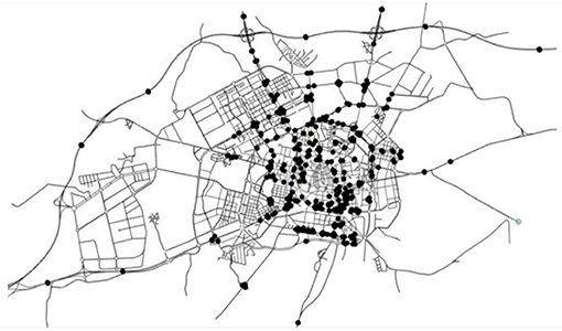
Figure 1. Network of Vitoria, Spain.

The mesoscopic simulator Aimsun (2017), a commercial software adopted by practitioners all over the world for planning and real-time management, has been adopted to map the OD flows to the traffic measurements through a Dynamic Traffic Assignment process. The simulations are run with a stochastic route choice scenario and path assignment fixed through dynamic user equilibrium.

In this experiment, the morning demand has been considered—from 7:00 a.m. to 12:00 p.m., for a total of 20 time intervals. Two different demand scenarios are considered, one resulting in an uncongested network (84,089 vehicles) and one resulting in a congested network (158,644 vehicles).

In the real-world experiment, PCA-LETKF results have been compared with those obtained with the LETKF model.

For the evaluation of the performance of the tested algorithms, the Normalized Root Mean Square (RMSN) error (19) is used, which has been previously chosen as the evaluation criteria in many research papers (Ashok and Ben-Akiva, 2000; Prakash et al., 2018).

$\begin{array}{ll}RMSN=\frac{\sqrt{n{\displaystyle {\sum }_{i=1}^n}{\left({ŷ}_i-y_i\right)}^2}}{{\displaystyle {\sum }_{i=1}^n}{y}_i}& (19)\end{array}$

Synthetic Experiments Results

Results in terms of estimated link flows and OD flows at the end of the model runs adopting the non-linear function (17) in the uncongested case are shown in Figure 2, where the red dashed line represents the initial error.

FIGURE 2

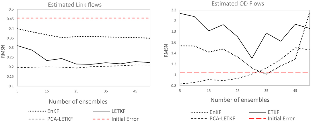
Figure 2. Error in terms of link flows (left) and OD flows (right) for each model.

In the figure, the x-axis represents the number of ensembles used by each model. Intuitively, larger values are associated with better predictions but also higher computational times. The y-axis indicates the quality of the prediction associated with a specific number of ensembles in terms of RMSN. As expected, both the LETKF and PCA-LETKF outperform the traditional EnKF. Despite being a quite advanced model capable of handling non-linearity, even when using 50 ensembles, the EnKF only reduces the error from 0.45 to 0.34 (black dotted line). It is also important to point out that—in order to capture non-linear phenomena—each ensemble requires to perform an objective function evaluation. This entails running the map linking OD flows to traffic counts 50 times for each time interval, one for each ensemble member. The main reason is that we only have 395 detectors to explain 3,249 variables. In similar conditions, the LETKF provides better results in terms of link flows, however, the PCA-LETKF (black dash-dotted line) performs better already with 5 ensembles, while the normal LETKF only provide good results (RMSN ≈ 0.2) for more than 25 ensembles, where again more ensembles mean more computational time. The reason is that as of now the LETKF is not exploiting any localization strategy. This means that more ensembles are needed to learn the structure of the data. Additionally, the PCA-LETKF also performs better in terms of OD flows for most of the cases. This usually happens for a low number of ensembles—between 5 and 25—which suggests that larger ensample values increase the probability of overfitting.

Comparing previous results with those obtained by the adoption of the non-linear function (18), it can be observed a similar pattern (Figure 3), with the PCA-LETKF model maintaining a constant RMSN value of ~0.2 (56% decrease from initial error) for the first function and of ~0.45 (65% decrease from initial error) for the second function. The estimated link flows error for the LETKF model decreases as the number of ensembles increases, until it converges to the results of PCA-LETKF for more than 20 ensemble members. This suggests that LETKF and PCA-LETKF potentially converge on similar results but also that LETKF is four times more demanding in terms of computational time.

FIGURE 3

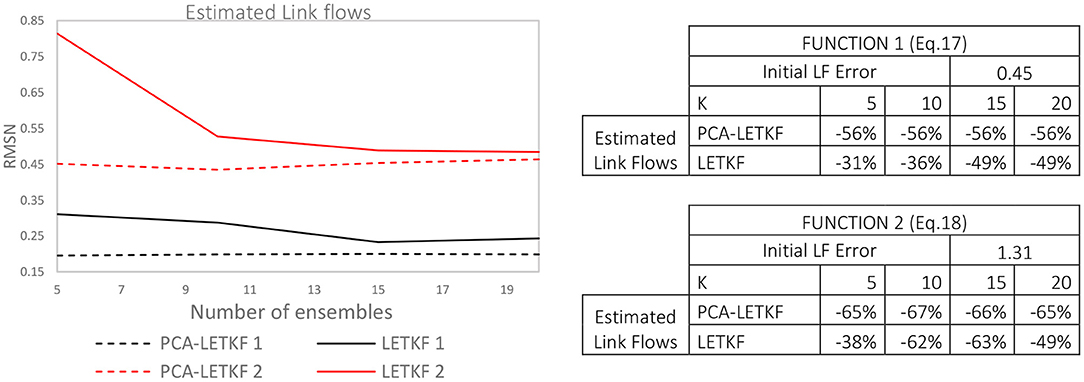
Figure 3. Error in terms of link flows for the two mapping functions.

Finally, Figures 2, 3 show a final error of 15–20%, which is too high for real time applications. Real-time applications usually start from a good historical matrix which is then corrected using models, such as the Kalman Filter. In Figures 2, 3, however, the initial error is 45%. This is unrealistic, as the Kalman filter will hardly manage to correct such a large error. To consider the impact of the initial (seed) matrix on the performances, the models have also been tested with function (17) considering varying degrees of randomization of the initial error between the real matrix and the seed matrix. A series of seed matrices has been created off the real matrix:

$\begin{array}{ll}{x}_{seed}^k=x_{real}\times (1-\frac{R*\Delta }{100})& (20)\end{array}$

where R is a normally distributed random vector with mean 0 and values ranging between 0 and the arbitrarily chosen parameter E, which represents the maximum percentage error given to each OD pair. Δ is a ±1 Bernoulli distribution random vector, which randomizes the reduction or the increase for each value OD pair.

In Figure 4 the results obtained with a 5-member ensemble and the maximum percentage error E given to the OD pairs ranging from 100 to 10% are shown.

FIGURE 4

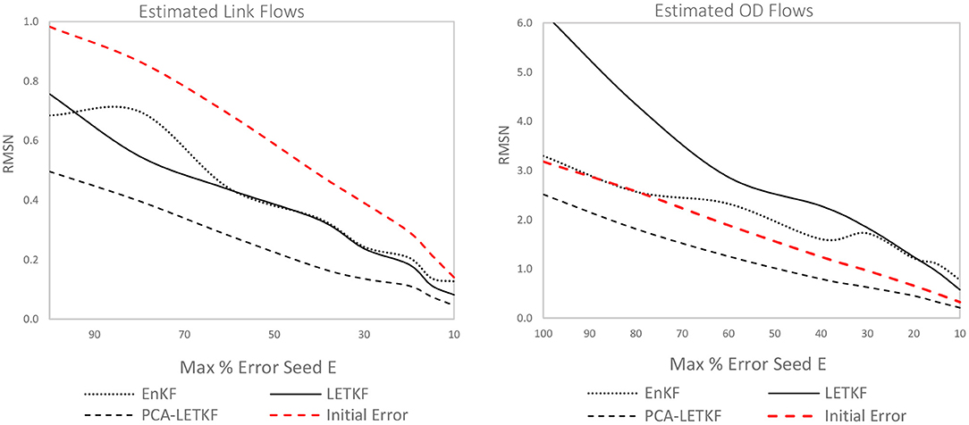
Figure 4. Error in terms of link flows (left) and OD flows (right) for each model using a 5-member ensemble.

It can be observed that the PCA-LETKF outperforms the other models, both in terms of link flows and OD flows, when 5 ensembles are used in the estimation. In particular, in terms of link flows, the LETKF results show a 22.5% improvement, when the maximum percentage error E between real and seed matrix is 100%, and a 42% improvement, when E is 10%. Whereas, the PCA-LETKF results show a 49.5% improvement for E = 100% and a 67% improvement for E = 10% in terms of link flows, and a 35% improvement in terms of OD flows.

The scatter chart of the results obtained for the 3 models using a 5-member ensemble and a starting maximum percentage error E of 15%, resulting in an initial link flows error of ~0.2, is highlighted in Figure 5. Figure 5A compares the values of the real OD matrix and the seed OD matrix, Figure 5B compares the values of the observed link flows and the simulated link flows obtained from the assignment of the initial seed matrix. Then, Figures 5C–E show the distance between the observed link flows and the estimated link flows obtained through EnKF, LETKF, and PCA-LETKF, respectively.

FIGURE 5

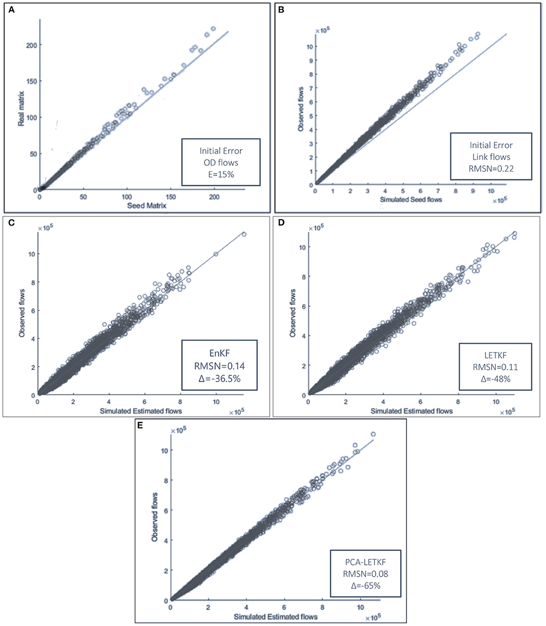
Figure 5. (A–E) Scatter chart of the error obtained with a 5-member ensemble and E = 15%.

Vitoria Network Results

We tested the PCA-LETKF for both congested and uncongested conditions. The results of the tests performed on the uncongested scenario are firstly presented in Figures 6, 7. The seed OD matrix has been created assuming a maximum percentage error E given to each OD pair of 50% from the real OD matrix, resulting in a starting RMSN between seed and real OD flows of 1.29 and a 0.34 RMSN between observed link flows and simulated link flows.

FIGURE 6

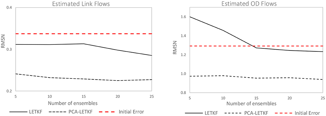
Figure 6. Error in terms of link flows (left) and OD flows (right) for the uncongested network.

FIGURE 7

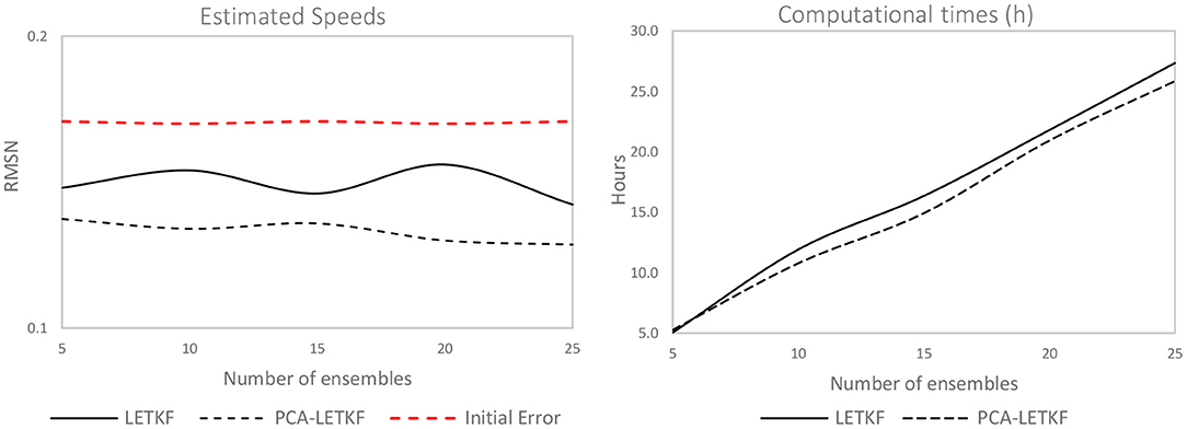
Figure 7. Error in terms of speeds (left) and computational times (right) for the uncongested network.

In terms of link flows, the LETKF algorithm shows a 9% improvement for a 5-member ensemble that increases up to 16% for a 25 member ensemble, whereas the PCA-LETKF's improvement stays in the 30–33% range regardless of the ensemble dimension. As for the OD flows, the LETKF algorithm presents unsatisfactory results, although the error seems to be decreasing for larger-sized ensembles. The PCA-LETKF, on the other hand, shows an improvement in terms of OD flows between 24 and 27%. Lastly, the LETKF algorithm presents an improvement in terms of observed speeds that ranges between 5 and 8%, whereas the PCA-LETKF presents a 11–14% improvement for the uncongested scenario.

The scatter chart of the results obtained for the models using a 5-member ensemble and a starting maximum percentage error E of 50%, resulting in an initial link flows error of 0.24, is highlighted in Figure 8. Figure 8A compares the values of the real OD matrix and the seed OD matrix, Figure 8B compares the values of the observed link flows and the simulated link flows obtained from the assignment of the initial seed matrix. Then, Figures 8C,D show the distance between the observed link flows and the estimated link flows obtained through PCA-LETKF and LETKF, respectively, while Figures 8E,F show the distance between the real OD flows and the estimated OD flows for the two models.

FIGURE 8

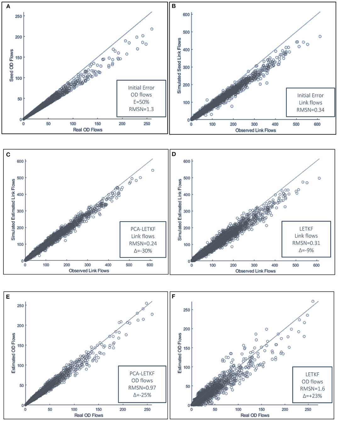
Figure 8. (A–F) Scatter chart of the error obtained with a 5 member ensemble and E = 50%.

The models have then been tested with varying degrees of reliability of the seed OD matrix, considering values of the maximum percentage error E between OD pairs that vary between 50 and 10%. The results are shown in Figures 9, 10. PCA-LETKF presents an improvement in term of link flows that varies between 28% (for a higher error between the real OD matrix and the seed OD matrix) and 47%, whereas the LETKF algorithm barely shows any improvement (4–9%) as 5 ensembles are way too little to statistically represent a large network, and the same applies to speeds. It follows that LETKF also fails to provide satisfactory results when it comes to OD flows, while the PCA-LETKF, instead, provides an improvement in terms of OD flows ranging between 24 and 35% and an improvement in terms of speeds between 11 and 14%.

FIGURE 9

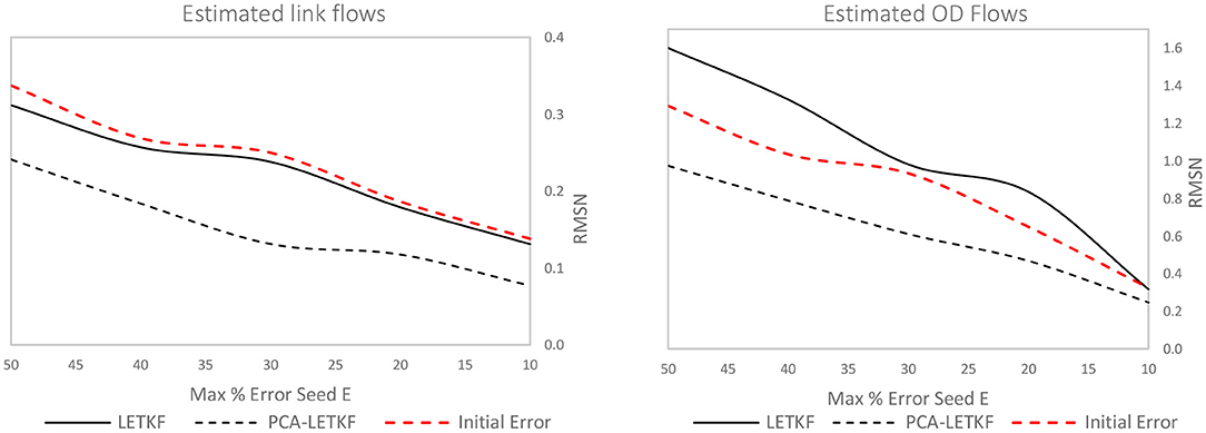
Figure 9. Error in terms of link flows (left) and OD flows (right) for each model using a 5-member ensemble.

FIGURE 10

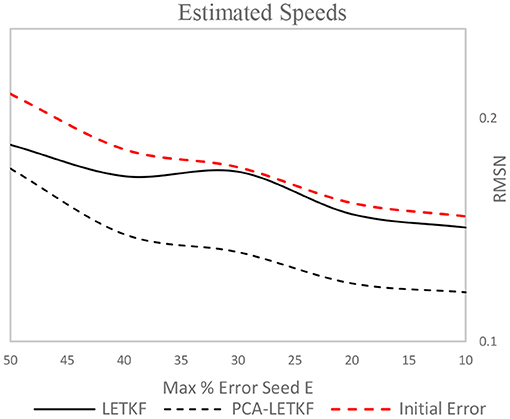
Figure 10. Error in terms of speeds for each model using a 5-member ensemble.

The same experiments have been repeated on the congested network, as shown in Figures 11, 12. The seed OD matrix has been created from the real OD matrix assuming a maximum percentage error of 15% given to each OD flow, even so, the initial error between the simulated link flows obtained from assigning the seed matrix onto the network and the observed counts is much higher than what has been observed for the uncongested scenario.

FIGURE 11

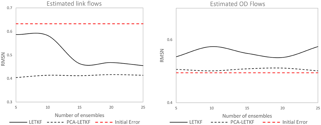
Figure 11. Error in terms of link flows (left) and OD flows (right) for the congested network.

FIGURE 12

Figure 12. Error in terms of speeds for the congested network.

Consistently with what has been observed on the synthetic network, the PCA-LETKF performance is more or less constant regardless of the size of the ensemble, whereas the LETKF model results are better when more members of the starting ensembles are used. In terms of link flows, the PCA-LETKF improves the RMSN by 34–36%, whereas the LETKF shows an improvement that goes from only 7–28% when 25 ensembles are used. In terms of OD flows, both algorithms show unsatisfactory results, with the PCA-LETKF not improving nor worsening the results compared to the seed matrix, unlike the LETKF model which shows a 10–16% increase of the RMSN between OD flows. As for speeds, the LETKF starts from a 2% improvement when 5 ensembles are used up to a 10% improvement when 25 ensembles are used, whereas the PCA-LETKF shows a 14–15% improvement. The scatter chart of the results obtained using 5 member ensembles are shown in Figure 13.

FIGURE 13

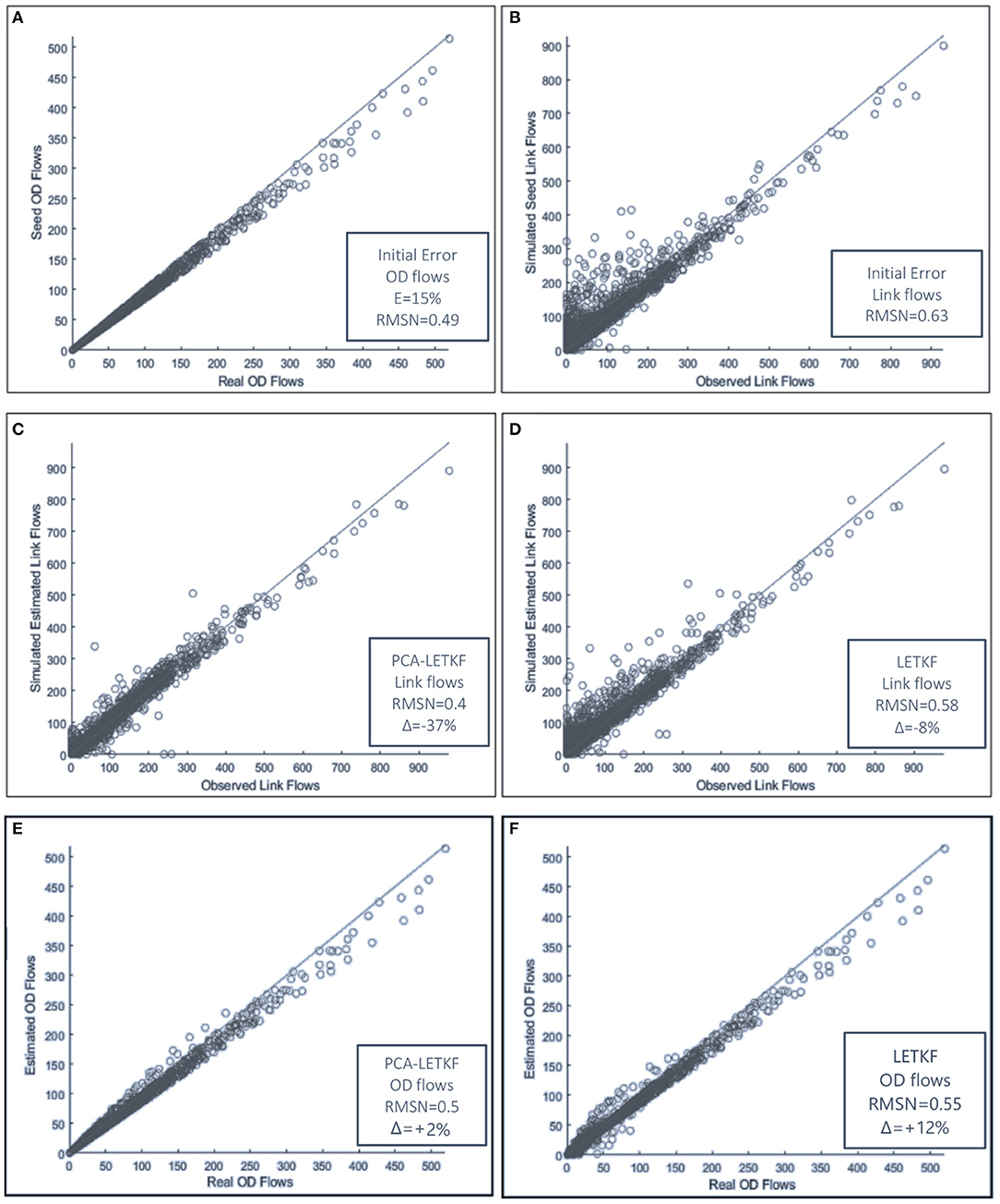
Figure 13. (A–F) Error in terms of link flows (left) and OD flows (right) for each model using a 5-member ensemble.

Lastly, LETKF and PCA-LETKF have then been tested with varying degrees of reliability of the seed OD matrix, with values of the maximum percentage error E between OD pairs starting from 15% and then going down to 3%, while the number of ensemble members is kept constant (k = 5) throughout the tests. Results are shown in Figures 14, 15.

FIGURE 14

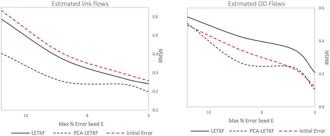
Figure 14. Error in terms of link flows (left) and OD flows (right) for each model using a 5-member ensemble.

FIGURE 15

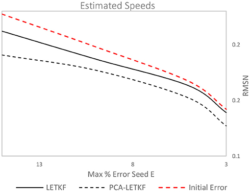
Figure 15. Error in terms of speeds for each model using a 5-member ensemble.

In terms of link flows, the PCA-LETKF results improve by 36–37% for E = 15% and E = 10% and by 20–22% for E = 5% and E = 3%, whereas the LETKF improvements stay in the 6–8% range throughout. As for OD flows, instead, the LETKF shows unsatisfactory results, whereas for the PCA-LETKF the results vary depending on the seed matrix: in some instances, the error between real OD flows and estimated OD flows is not higher nor lower than the starting error, while in other instances improvements up to 22% are observed. As for speeds, the error decreases from 2 to 6% for the LETKF algorithm and between 9 and 14% for the PCA-LETKF algorithm.

Conclusions

This paper introduces a ODDE approach that combines Principal Component Analysis and the Local Ensemble Transformed Kalman Filter (PCA-LETKF). The advantages of this approach are 2-fold:

- PCA-LETKF does not require an analytical formulation of the assignment matrix, which is implicitly captured by the DTA simulator. This means that multiple data sources can be utilized in the measurement equations. In this work, traffic counts and speeds have been utilized, but the approach allows for other sources, such as FCD.

- PCA-LETKF exploits the “local” peculiarity of LETKF algorithm by finding the spatial correlation that exists between the variables, through the implementation of the Principal Component Analysis to reduce the dimensionality of the problem. In the case studies presented in this thesis, the initial 3,249 variables x to estimate have been reduced to 195 variables z, which contain 95% of the variance. The dimensionality of the problem has been thus reduced by 17 times.

Reducing the dimensionality of the problem tackles two major issues when it comes to the applicability of ensemble Kalman filters to online applications: computational times and undersampling. Computational time, for the online dynamic OD estimation, is a major constraint which generally make ensemble-based filters impractical for anything but very small networks. For a medium-large sized network like the network of the city of Vitoria, both the EnKF and LETKF require a large ensemble to correctly explain the system dynamics, making them computationally unfeasible for online applications, as every ensemble member requires a run of the DTA simulator—the most computationally expensive part of the model. Additionally, deciding the right number of ensembles is a challenging task. Both the EnKF and LETKF show that a small number of ensembles is not sufficient to generate accurate predictions while a large number leads to overfitting. The PCA-LETKF, on the other hand, is much more robust in terms of outputs and less prone to overfitting.

The PCA-LETKF approach shows positive results that outperform those of the EnKF and LETKF for as low as 5 ensembles members, with the estimation of the OD flows over a 5-h long time horizon taking about 5 h as well, meaning that the estimation process of the OD flows of a single time interval takes roughly the same amount of time of the interval itself.

One of the limits of ensemble-based Kalman filters is that if an ensemble that is too small to statistically represent the state and span the sub-space adequately is chosen, the system will be undersampled, which generally leads to a series of unwanted errors affecting the performance of the ensemble filters (spurious correlation, inbreeding, filter divergence). This explains the unsatisfactory results of EnKF and LETKF when it comes to correctly estimate the OD flows, using small ensembles. As for PCA-LETKF, instead, its variables z (the Principal Components) already contain the information of 100 data samples computed beforehand (i.e., the outputs of 100 previous offline calibrations), hence why for all the tests conducted on both the synthetic and the Vitoria network, PCA-LETKF outperforms both EnKF and LETKF. The tests show good results when it comes to better predict the actual traffic conditions on the network. As for OD flows, the EnKF and LETKF show unsatisfactory results for small ensembles, whereas the PCA-LETKF's results are mixed.

The way traffic counts and speeds—whose variances can be very different—are jointly inserted in the equations could be fine-tuned to better exploit the role that speeds play into representing actual traffic conditions when it comes to congested networks. All kinds of data can be incorporated in the proposed model, however, so far, we have only addressed how to incorporate data on a link-level scale, whereas the incorporation of point-to-point data, such as travel times, could be a future development. Furthermore, the assignment part of the algorithm could be also speed up further. In the transition equations, a simple polynomial interpolation has been used to forecast the variables from one time interval to the next, as the definition of the best-possible transition equation is outside the scope of this paper. However, several autoregressive models have been already proposed in literature and many more have yet to be applied to the OD estimation problem specifically, such as Gaussian processes, for example. Therefore, future developments will cover an evaluation of the best approach to maximize predictive performance of PCA-LETKF. Lastly, an optimal covariance inflation factor could be defined for the Victoria network, as it has only been tested for the synthetic experiment.

Data Availability Statement

The original contributions generated for the study are included in the article/Supplementary Material, further inquiries can be directed to the corresponding author/s.

Author Contributions

All authors listed have made a substantial, direct and intellectual contribution to the work, and approved it for publication.

Conflict of Interest

The authors declare that the research was conducted in the absence of any commercial or financial relationships that could be construed as a potential conflict of interest.

Acknowledgments

The authors would like to thank Aimsun for providing them with the calibrated Vitoria network.

References

Aimsun (2017). Aimsun Next 8.2 User's Manual. Barcelona: Aimsun. Available online at: https://www.scribd.com/document/266245543/Aimsun-Users-Manual-v8 (accessed June 12, 2018).

Anderson, J. L., and Anderson, S. L. (1999). A Monte Carlo implementation of the nonlinear filtering problem to produce ensemble assimilations and forecasts. Mon. Weather Rev. 127, 2741–2758. doi: 10.1175/1520-0493(1999)127<2741:AMCIOT>2.0.CO;2

CrossRef Full Text | Google Scholar

Antoniou, C., Azevedo, C. L., Lu, L., Pereira, F., and Ben-Akiva, M. (2015). W-spsa in practice: approximation of weight matrices and calibration of traffic simulation models. Transport. Res. C Emerg. Technol. 59, 129–146. doi: 10.1016/j.trc.2015.04.030

CrossRef Full Text | Google Scholar

Antoniou, C., Ben-Akiva, M., and Koutsopoulos, H. (2007). Nonlinear Kalman filtering algorithms for on-line calibration of dynamic traffic assignment models. IEEE Trans. Intell. Transport. Syst. 8, 661–670. doi: 10.1109/TITS.2007.908569

CrossRef Full Text | Google Scholar

Ashok, K. (1996). Estimation and prediction of time-dependent origin destination flows (Ph.D. thesis), Massachusetts Institute of Technology, Cambridge, MA, United States.

Google Scholar

Ashok, K., and Ben-Akiva, M. (1993). “Dynamic origin-destination matrix estimation and prediction for real-time traffic management systems,” in Proceedings of the 12th ISTTT Transportation and Traffic Theory (Berkeley, CA: Elsevier Science Publishing).

Google Scholar

Ashok, K., and Ben-Akiva, M. E. (2000). Alternative approaches for real-time estimation and prediction of time-dependent origin–destination flows. Transport. Sci. 34, 21–36. doi: 10.1287/trsc.34.1.21.12282

CrossRef Full Text | Google Scholar

Balakrishna, R., Antoniou, C., Ben-Akiva, M., Koutsopoulos, H., and Wen, Y. (2007). Calibration of microscopic traffic simulation models: methods and application. Transport. Res. Rec. 1999, 198–207. doi: 10.3141/1999-21

CrossRef Full Text | Google Scholar

Barcelo, J., and Montero, L. (2015). A robust framework for the estimation of dynamic OD trip matrices for reliable traffic management. Transport. Res. Proc. 10, 134–144. doi: 10.1016/j.trpro.2015.09.063

CrossRef Full Text | Google Scholar

Behara, K. N. S., Bhaskar, A., and Chung, E. (2020). A novel approach for the structural comparison of origin-destination matrices: Levenshtein distance. Transport. Res. C Emerg. Technol. 111, 513–530. doi: 10.1016/j.trc.2020.01.005

CrossRef Full Text | Google Scholar

Bierlaire, M., and Crittin, F. (2004). An efficient algorithm for real-time estimation and prediction of dynamic OD tables. Oper. Res. 52, 116–127. doi: 10.1287/opre.1030.0071

CrossRef Full Text | Google Scholar

Bishop, C. H., Etherton, B. J., and Majumdar, S. J. (2001). Adaptive sampling with the ensemble transform Kalman filter. Part I: theoretical aspects. Mont. Weather Rev. 129, 420–436. doi: 10.1175/1520-0493(2001)129<0420:ASWTET>2.0.CO;2

CrossRef Full Text | Google Scholar

Cantelmo, G., Cipriani, E., Gemma, A., and Nigro, M. (2014). An adaptive bi-level gradient procedure for the estimation of dynamic traffic demand. IEEE Trans. Intell. Transport. Syst. 15, 1348–1361. doi: 10.1109/TITS.2014.2299734

CrossRef Full Text | Google Scholar

Cantelmo, G., Qurashi, M., Prakash, A., Antoniou, C., and Viti, F. (2019). Incorporating trip chaining within online demand estimation. Transport. Res. B Methodol. 132, 171–187. doi: 10.1016/j.trpro.2019.05.025

CrossRef Full Text | Google Scholar

Cantelmo, G., and Viti, F. (2020). A big data demand estimation model for urban congested networks. Transport Telecommun. J. 21, 245–254. doi: 10.2478/ttj-2020-0019

CrossRef Full Text | Google Scholar

Carrese, S., Cipriani, E., Mannini, L., and Nigro, M. (2017). Dynamic demand estimation and prediction for traffic urban. Transport. Res. C 81, 83–98. doi: 10.1016/j.trc.2017.05.013

CrossRef Full Text | Google Scholar

Cascetta, E. (1984). Estimation of trip matrices from traffic counts and survey data: a generalized least squares estimator. Transport. Res. B 8, 289–299. doi: 10.1016/0191-2615(84)90012-2

CrossRef Full Text | Google Scholar

Cascetta, E., Inaudi, D., and Marquis, G. (1993). Dynamic estimators of origin-destination matrices using traffic counts. Transport. Sci. 27, 363–373. doi: 10.1287/trsc.27.4.363

CrossRef Full Text | Google Scholar

Chang, G.-L., and Wu, J. (1994). Recursive estimation of time-varying origin-destination flows from traffic counts in freeway corridors. Transport. Res. B Meth. 28, 141–160. doi: 10.1016/0191-2615(94)90022-1

CrossRef Full Text | Google Scholar

Cipriani, E., and Nigro, M. (2017). Dynamic Travel Demand Estimation and Prediction Methods. New York, NY: Nova Science Publishers, Inc.

Djukic, T., Van Lint, J., and Hoogendoorn, S. (2012). Application of principal component analysis to predict dynamic origin–destination matrices. Transport. Res. Rec. 2283, 81–89. doi: 10.3141/2283-09

CrossRef Full Text | Google Scholar

Evensen, G. (2003). The Ensemble Kalman Filter: theoretical formulation and practical implementation. Ocean Dyn. 53, 343–367. doi: 10.1007/s10236-003-0036-9

CrossRef Full Text | Google Scholar

Frederix, R., Viti, F., Corthout, R., and Tampère, C. (2011). New gradient approximation method for dynamic origin-destination matrix estimation on congested networks. Transport. Res. Rec. 2263, 19–25. doi: 10.3141/2263-03

CrossRef Full Text | Google Scholar

Frederix, R., and Viti, F. Tampère, M. J. (2013). Dynamic origin-destination estimation in congested networks: theoretical findings and implications in practice. Transportmetrica 9, 494–513. doi: 10.1080/18128602.2011.619587

CrossRef Full Text | Google Scholar

Furrer, R., and Bengtsson, T. (2007). Estimation of high-dimensional prior and posterior covariance matrices in Kalman filter variants. J. Multivar. Anal. 98, 227–255. doi: 10.1016/j.jmva.2006.08.003

CrossRef Full Text | Google Scholar

Hamill, T., Whitaker, J. S., and Snyder, C. (2001). Distance-dependent filtering of background error covariance estimates in an ensemble Kalman filter. Mon. Weather Rev. 129, 2776–2790. doi: 10.1175/1520-0493(2001)129<2776:DDFOBE>2.0.CO;2

CrossRef Full Text | Google Scholar

Hunt, B. R., Kostelich, E. J., and Szunyogh, I. (2007). Efficient data assimilation for spatiotemporal chaos: A local ensemble transform Kalman filter. Phys. D Nonlin. Phenom. 230, 112–126. doi: 10.1016/j.physd.2006.11.008

CrossRef Full Text | Google Scholar

Jolliffe, I. (2002). Principal Component Analysis, 2nd Edn. New York, NY: Springer-Verlag.

Google Scholar

Kalman, R. E. (1960). A new approach to linear filtering and prediction problems. J. Basic Eng. 82:35. doi: 10.1115/1.3662552

CrossRef Full Text | Google Scholar

Kalnay, E. (2002). Atmospheric Modeling, Data Assimilation and Predictability. Cambridge: Cambridge University Press. doi: 10.1017/CBO9780511802270

CrossRef Full Text | Google Scholar

Krishnakumari, P., Lint, J. W. C., Djukic, T., and Cats, O. (2019). A data driven method for OD matrix estimation. Transport. Res. C Emerg. Technol. 132, 171–187. doi: 10.1016/j.trpro.2019.05.009

CrossRef Full Text | Google Scholar

Liu, J., Zheng, F., van Zuylen, H., and li, J. (2020). A dynamic OD prediction approach for urban networks based on automatic number plate recognition data. Transport. Res. Proc. 47, 601–608. doi: 10.1016/j.trpro.2020.03.137

CrossRef Full Text | Google Scholar

Lorenc, A. C. (2003). The potential of the ensemble Kalman filter for NWP—a comparison with 4D-Var. Q. J. R. Meteorol. Soc. 129, 3183–3203. doi: 10.1256/qj.02.132

CrossRef Full Text | Google Scholar

Marzano, V., Papola, A., and Simonelli, F. (2009). Limits and perspectives of effective o–d matrix correction using traffic counts. Transport. Res. C Emerg. Technol. 17, 120–132. doi: 10.1016/j.trc.2008.09.001

CrossRef Full Text | Google Scholar

Marzano, V., Papola, A., Simonelli, F., and Papageorgiou, M. (2018). A Kalman filter for quasi-dynamic O-D flow estimation/updating. IEEE Trans. Intell. Transport. Syst. 19, 3604–3612. doi: 10.1109/TITS.2018.2865610

CrossRef Full Text | Google Scholar

Oke, P. R., Sakov, P., and Corney, S. P. (2007). Impacts of localisation in the EnKF and EnOI: experiments with a small model. Ocean Dyn. 57, 32–45. doi: 10.1007/s10236-006-0088-8

CrossRef Full Text | Google Scholar

Okutani, I., and Stephanedes, Y. (1984). Dynamic prediction of traffic volume through Kalman filtering theory. Transport. Res. B 18, 1–11. doi: 10.1016/0191-2615(84)90002-X

CrossRef Full Text | Google Scholar

Prakash, A. A., Seshadri, R., Antoniou, C., Pereira, F. C., and Ben-Akiva, M. (2018). Improving scalability of generic online calibration for real-time dynamic traffic assignment systems. Transport. Res. Rec. 2672, 79–92. doi: 10.1177/0361198118791360

CrossRef Full Text | Google Scholar

Qurashi, M., Ma, T., Chaniotakis, E., and Antoniou, C. (2019). PC–SPSA: employing dimensionality reduction to limit SPSA search noise in DTA model calibration. IEEE Trans. Intell. Transport. Syst. 21, 1635–1645. doi: 10.1109/TITS.2019.2915273

CrossRef Full Text | Google Scholar

Styblinski, M. A., and Tang, T. S. (1990). Experiments in nonconvex optimization: Stochastic approximation with function smoothing and simulated annealing. Neural Netw. 3, 467–483. doi: 10.1016/0893-6080(90)90029-K

CrossRef Full Text | Google Scholar

Van der Zijpp, N., and Hammerslag, R. (1994). Improved Kalman filtering approach for estimating origin-destination matrices for freeway corridors. Transport. Res. Rec. 1443, 54–64.

Google Scholar

Wang, X., Bishop, C. H., and Julier, S. J. (2004). Which is better, an ensemble of positive–negative pairs or a centered spherical simplex ensemble? Mon. Weather Rev. 132, 1590–1605. doi: 10.1175/1520-0493(2004)132<1590:WIBAEO>2.0.CO;2

CrossRef Full Text | Google Scholar

Whitaker, J. S., and Hamill, T. M. (2002). Ensemble data assimilation without perturbed observations. Mon. Weather Rev. 130, 1913–1924. doi: 10.1175/1520-0493(2002)130<1913:EDAWPO>2.0.CO;2

CrossRef Full Text | Google Scholar

Xia, J., Dai, W., Polak, J., and Bierlaire, M. (2018). Dimension reduction for origin-destination flow estimation: blind estimation made possible. arXiv 1810.06077 [cs].

Google Scholar

Yang, X., Lu, Y., and Hao, W. (2017). Origin-destination estimation using probe vehicle trajectory and link counts. J. Adv. Transport. 2017:4341532. doi: 10.1155/2017/4341532

CrossRef Full Text | Google Scholar

Zhang, H., Seshadri, R., Akkinepally, A., Pereira, F., Antoniou, C., and Ben-Akiva, M. (2017). Improved calibration method for dynamic traffic assignment models: constrained extended Kalman filter. Transport. Res. Rec. 2667, 142–153. doi: 10.3141/2667-14

CrossRef Full Text | Google Scholar

Zhou, X., and Mahmassani, H. (2007). A structural state space model for real-time traffic origin–destination demand estimation and prediction in a day-to-day learning framework. Transport. Res. B 41, 823–840. doi: 10.1016/j.trb.2007.02.004

CrossRef Full Text | Google Scholar