Quantifying nonlinear responses of vegetation to hydro-climatic changes in mountainous Southwest China

Vegetation plays an essential role in terrestrial carbon balance and climate systems. Exploring and understanding relationships between vegetation dynamics and climate changes in Southwest China is of great significance for ecological environment conservation. Nonlinear relationships between vegetation and natural factors are extraordinarily complex in Southwest China with complicated topographic conditions and changeable climatic characteristics. Considering the complex nonlinear relationships, the Random Forest (RF) and an integration of Convolutional Neural Networks and Long Short-Term Memory network (CNN-LSTM) were used with multi-source data from 2000–2020. Performance of two models were compared with precision indicators, and influence of topographic and hydro-climatic factors on vegetation was quantified based on the optimal models. Results revealed that the Normalized Difference Vegetation Index had a significant negative correlation with elevation and a positive correlation with land surface temperature and evapotranspiration. According to precision indicators, the RF model (RF3) built with longitude, latitude, elevation, slope, temperature, precipitation, evapotranspiration and surface solar radiation as inputs outperformed other models. Relative importance of the eight natural factors was quantified based on the RF3, and results indicated that elevation, temperature and evapotranspiration were major factors that influenced vegetation growth. Responses of vegetation toward climatic variables exhibited significant seasonal change, and there were different decisive factors, which influenced vegetation growth in forests, grasslands and croplands.

1 Introduction

Vegetation is one of the most important components of terrestrial ecosystems and plays an essential role in terrestrial carbon balance and climate systems (Zhang et al., 2021). Remote sensing technology can provide temporal and spatial dynamic observations of vegetation at large scales, and has been widely used to monitor vegetation growth (Chen et al., 2018). Based on satellite remote sensing, the Normalized Difference Vegetation Index (NDVI) can reflect characteristics of surface vegetation and monitor dynamic changes of vegetation, and has been the most widely used indicator for monitoring vegetation (Hou et al., 2015; Piao et al., 2020).

Major driving factors of vegetation change at a large scale have received extensive attention for decades (Liu et al., 2018; Piao et al., 2020; Yin et al., 2020). Relationships between vegetation and climate change are extremely complicated and characterized by spatial heterogeneity, especially in the mountainous Southwest China (Liu et al., 2018; Zhang et al., 2021). The terrain in Southwest China is very complicated, and influences of climate change on vegetation in this region vary spatiotemporally. In the eastern area, including southwestern Yunnan, eastern Guizhou and central Sichuan, vegetation coverage was very high and vegetation appeared a significant upward trend, though precipitation showed a decreased tendency in Southwest China after 2000 (Duan et al., 2022). The ecosystem in areas at the junction of Sichuan, Tibet, and Yunnan provinces was very sensitive to climate change, and vegetation was significantly correlated with temperature and precipitation (Lai et al., 2023). Especially in parts of Yunnan Province with fragile ecological environments, improving temperature at short time scales had a certain adverse influence on vegetation growth (Liu et al., 2018).

In previous researches, links between vegetation and climatic variables were investigated most by adopting statistical linear methods, such as multivariate regression analysis and correlation analysis (Camberlin et al., 2007; Muir et al., 2021; Wang et al., 2021). Camberlin et al. (2007) computed linear correlations and regressions between vegetation and annual rainfall, and found that vegetation had a high correlation with rainfall in semi-arid zones and a weaker response in sub-humid and humid climates. However, these methods were not always able to take into account the spatial and temporal variations of variables and mostly ignored nonstationary relationships between variables, both of which were essential for exactly analyzing relationships between vegetation and climate variability (Foody, 2003; Li et al., 2013; Georganos et al., 2017). Spatial autocorrelation of variables had a detrimental effect on results of statistical analysis (Muir et al., 2021). As a result, quantifying complex nonlinear responses under linear assumption or ignoring combined effects of topographic and climatic factors could overestimate or underestimate influences of variant variables.

Machine learning has a superiority in responding to these problems and been widely used to explore complex nonlinear relationships among topographic conditions, climate change and vegetation growth (Chen et al., 2020; Zafar et al., 2023). For example, the Random Forest model has distinct advantages in fitting higher dimensional data and can quantify relative importance of input variables (Leo, 2001; Chen et al., 2022; Zafar et al., 2023). As a branch of machine learning, deep learning can automatically learn robust feature representations and shows great potential in many fields. Three main deep learning architectures include Convolutional Neural Networks (CNN), Recurrent Neural Networks (RNN), and Self-Attention Networks (or Transformers). The CNN is able to perform convolutional operations on time series to extract local features, but is not sensitive to temporal characters of data (Cao et al., 2022). RNN is a neural network with strong adaptability to temporal data. As a kind of advanced RNN, Long Short-Term Memory (LSTM) can effectively handle long-term dependencies in time series data, and is applied extensively for sequence data representation (Zhao et al., 2021; Ma and Liang, 2022; Wang et al., 2023). Integrating CNN and LSTM can maintain the capability of CNN for capturing information and the sensitivity of LSTM to time series data, and improve performance of the models.

Exploring and understanding relationships between vegetation dynamics and climate changes in Southwest China is of great significance for ecological environment conservation. In the current paper, the Random Forest and an integration of CNN and LSTM network were used to explore nonlinear relationships between vegetation dynamics and climate change and quantify contributions of topography and hydro-climatic factors to vegetation growth in Southwest China with a complicated topographic feature.

2 Materials and methods

2.1 Study area

The study area is located in southwest China and mainly composed of Chongqing, Sichuan, Guizhou, Yunnan and a small part of Tibet province (Figure 1). The surface condition is very complicated in the mountainous study area covered by the Sichuan Basin, the Yunnan-Guizhou Plateau, and the southeastern Qinghai Tibet Plateau. The terrain is characterized by severe undulations and a descending gradient from west to east, with elevations ranging from 100 to 7,002 m.

Figure 1

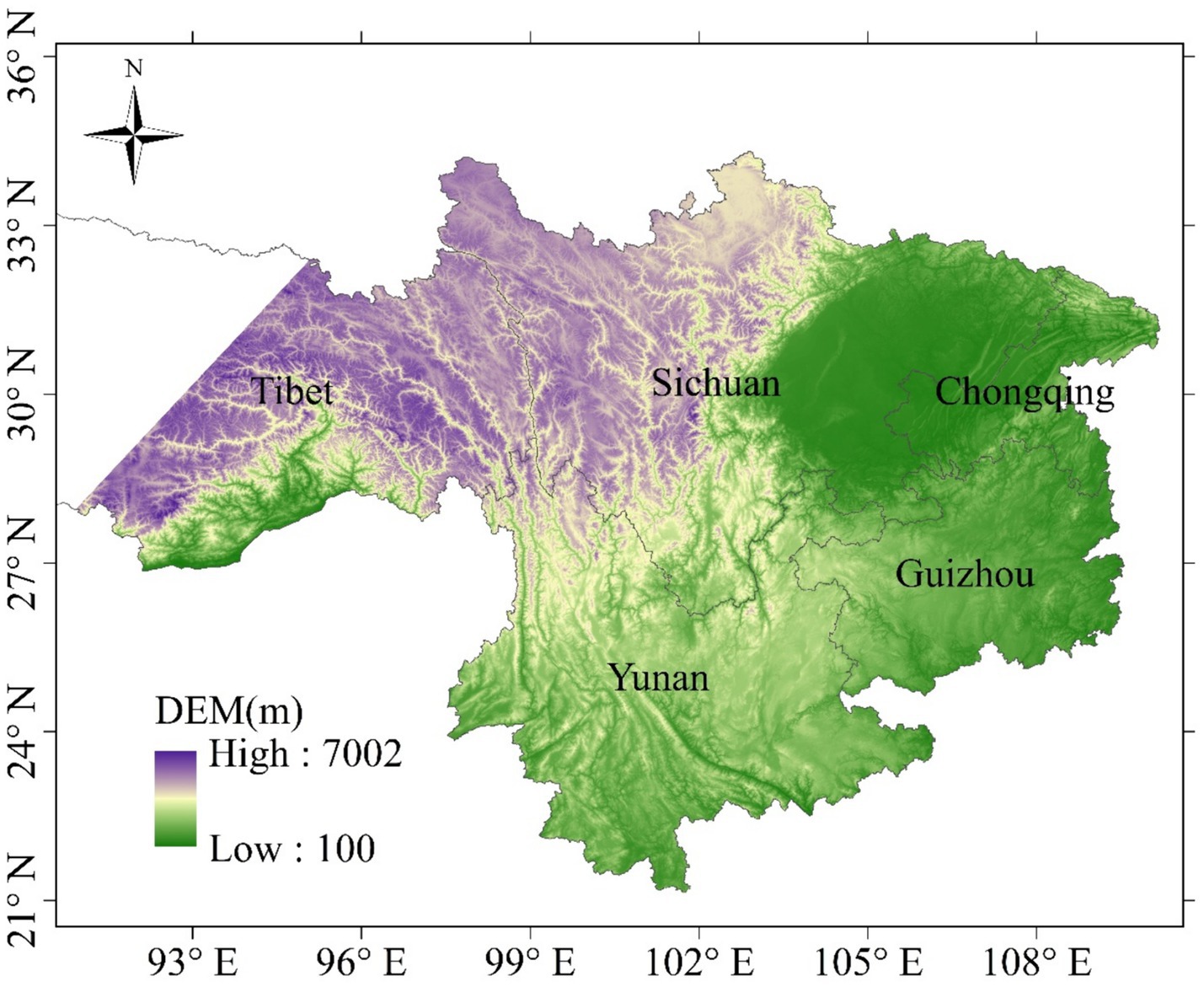
Figure 1. Map of digital elevation model (DEM) in the study area.

The climate is mainly subtropical and temperate. The study area has a humid mid-subtropical monsoon climate in the Sichuan Basin and a subtropical and tropical monsoon climate in the Yunnan-Guizhou Plateau. Spatiotemporal distribution of precipitation in the region is markedly uneven, with annual precipitation decreasing from southeast to northwest. The average annual precipitation in this area varies between 600 and 2,300 mm. Due to complex geography, spatial distribution of temperature in this area is obviously various, with annual average temperature exceeding 18°C. The Qinghai Tibet Plateau generally experiences lower annual temperatures compared to the Yunnan-Guizhou Plateau and the Sichuan Basin.

Grasslands and forests dominate the land use types in the southwestern mountainous area (Figure 2). Grasslands constitute 60.8% of the study area, predominantly located in northeast Tibet and northwest Sichuan. Forests account for 24.1%, mainly distributed in Yunnan, Sichuan and southern Xizang. Croplands are located mainly in the Sichuan Basin. Due to diversities of climate and terrain in the region, vegetation types are also very abundant.

Figure 2

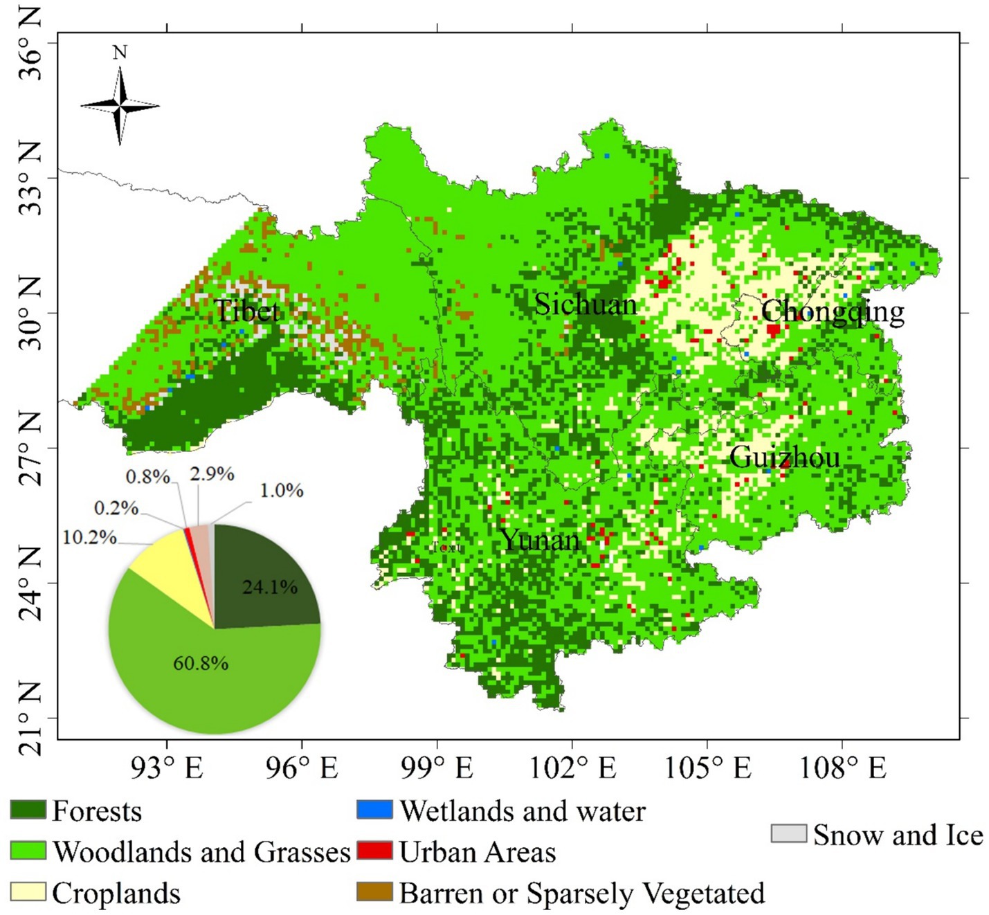
Figure 2. Map of land use types in 2020.

2.2 Materials

Hydro-climatic data from the Global Land Data Assimilation System (GLDAS), the Moderate Resolution Imaging Spectroradiometer (MODIS) and surface solar radiation synthetic dataset (Rs) with a resolution of 10 km from National Tibetan Plateau/Third Pole Environment Data Center¹ were used to analyze influences of hydro-climatic factors on vegetation change. The Digital Elevation Model (DEM) derived from NASA’s Shuttle Radar Topography Mission (SRTM) with a spatial resolution of 90 m was used as a terrain parameter. Details of multi-source data used in this paper are listed in Table 1.

Table 1

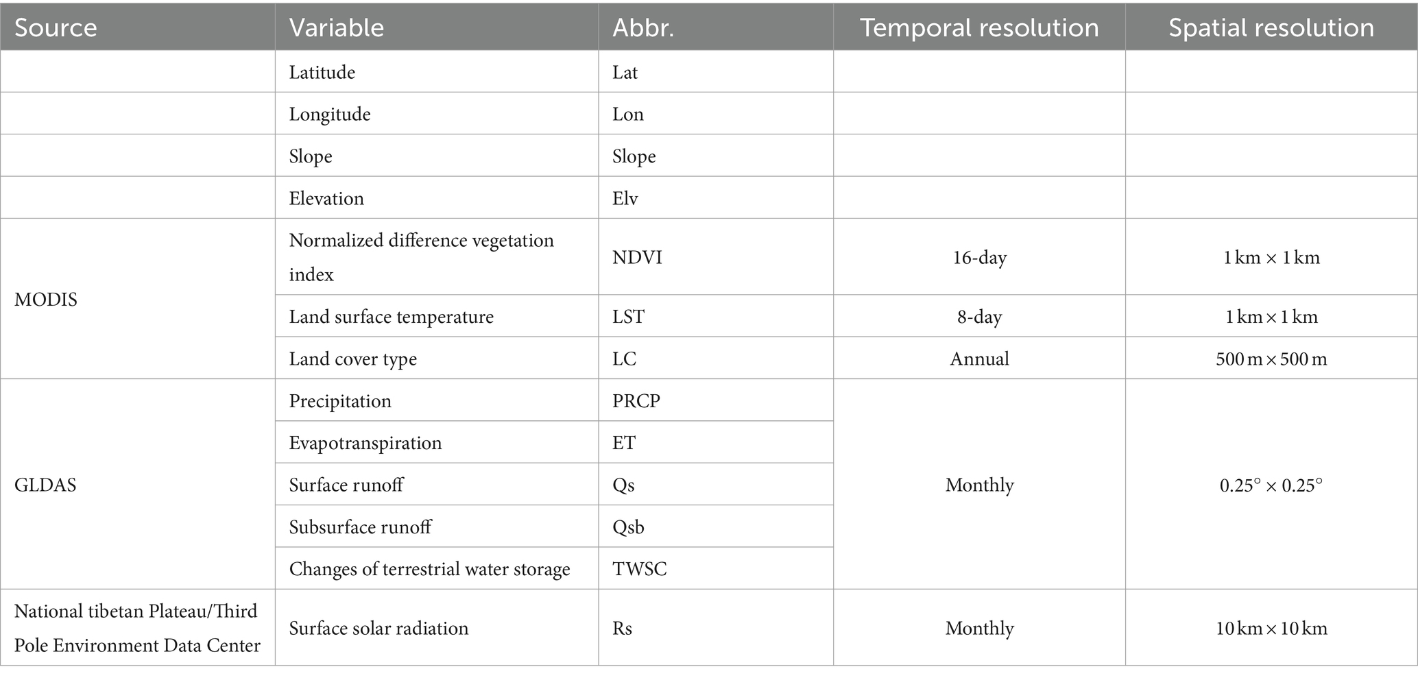
Table 1. Variables and data sources.

2.2.1 MODIS

The 16-day Normalized Difference Vegetation Index (NDVI) product (MOD13A2), 8-day land surface temperature (LST) product (MOD11A2) with a resolution of 1 km × km and annual land cover product (MCD12Q1) with a resolution of 500 m × 500 m from 2000–2020 are available from the MODIS. The standard NDVI values range from −1 to 1, and standardized pixels of NDVI data below 0.1 represent rocks, human-made structures, clouds, water, and snow (Worku et al., 2023). Based on the International Geosphere Biosphere Programme, land cover types were classified into 7 categories, including forests, woodlands and grasses, croplands, water and permanent wetlands, urban areas, barren or sparsely vegetated and snow and ice.

The data have multiple temporal and spatial resolutions. The datasets used in this paper were extracted and resampled at a 0.25° × 0.25° spatial resolution with the bilinear interpolation. The Maximum Value Composite method was used to generate monthly composite NDVI and LST and minimize atmospheric effects.

2.2.2 GLDAS

The GLDAS is a surface modeling system, which integrates global satellite and ground observation data to drive advanced simulations of climate and hydrological surveys (Moghim, 2020). It utilizes data assimilation to input satellite data and ground observation data into advanced surface models (LSMs), including Noah, Variable Infiltration Capacity (VIC), Mosaic and Common Land Model (CLM), to provide surface state and flux.

In this paper, monthly GLDAS products with a spatial resolution of 0.25^o × 0.25^o from 2002 to 2020, mainly including precipitation (PRCP), evapotranspiration (ET), surface and subsurface runoff (Qs and Qsb) were used. According to the theory of water balance, monthly terrestrial water storage changes (TWSC) were derived with monthly PRCP, ET, Qs and Qsb (Chen et al., 2020). The Equation (1) is as follows:

$\begin{array}{ll}TWSC=P-ET-Qs-Qsb& (1)\end{array}$

2.3 Methods

Based on multi-source data, responses of vegetation growth to natural factors were explored with correlation analysis, Random Forest (RF) and the integration of CNN and LSTM network (CNN-LSTM). The RF and CNN-LSTM were realized for distinguishing contributions of hydro-climatic factors in the study area.

2.3.1 Correlation analysis

The Spearman’s rank correlation coefficient (r) was a non-parametric measure of correlation. In the current paper, it was utilized to examine relationships between vegetation growth and natural variables and tested with a two-tailed Student’s t-test.

2.3.2 Random forest

Exploring nonlinear relationships among complicated terrains, varied climate and vegetation growth presents significant challenges. The Random Forest has a strong advantage in uncovering subtle nonlinear relationships and can quantify relative importance of various variables with the increased mean squared error (%IncMSE), combining benefits of interpretability and flexibility (Leo, 2001). Hence, Random Forest was used to build relational models with NDVI as a dependent variable and natural factors, including 4 topographic factors (longitude (Lon), latitude (Lat), elevation (Elv) and Slope) and 7 hydro-climatic factors (LST, PRCP, ET, Qs, Qsb, TWSC and Rs) as independent variables.

Random Forest (RF) integrates multiple weak classifiers and adopts the ensemble method to enhance the overall model’s predictive performance and generalization capability. The out-of-bag error estimate is unbiased and one of important advantages of random forest. Random forest randomly selects subsets of features used in each data sample to build full decision trees, and the randomness plays a crucial role to mitigating the risk of bias. To ensure robustness of random forest and alleviate overfitting, 80% of data were randomly selected and employed for constructing models and the others were used to validate model performance.

The ntree and mtry are important parameters in random forest. The ntree is number of trees and set to 500. The mtry is number of candidates draw to feed the algorithm and set to 2–4 in current paper. RF models were built repeatedly with different input variables and parameters for obtaining the final model with higher accuracy based on the cross-validation. The RF models were operated in the R package “randomForest”.

2.3.3 Integrated CNN-LSTM network

Traditional RNN encounters problems of gradient explosion or gradient vanishing when dealing with long sequences, and has difficulty learning long-term dependencies. Special structural design in LSTM can effectively alleviate these problems, and thereby LSTM can better handle long sequence data. The LSTM model is based on the assumption that not all information is equally important. Based on the assumption, LSTM can identify important information and remember it for the long term, and identify unimportant information to forget through the internal gating mechanism.

Similarly, four topographic factors and seven hydro-climatic factors were used to build the integrated CNN-LSTM models (Li et al., 2022; Gao et al., 2023), and 80% of data were used as the training set and 20% of them for validation. The integrated CNN-LSTM network (CNN-LSTM) consists of two parts. The CNN model was used to traverse topographic and climatic data with convolutional layers, and the LSTM was utilized to capture features from the convolutional layer. In order to increase the nonlinear representation of the model, the activation function, namely ReLU, was used to nonlinearly transform outputs from the convolutional layer. The mean absolute error was served as model loss values in the CNN-LSTM models. The CNN-LSTM network was built with the Pytorch platform.

2.3.4 Precision indicators

As shown in Equations (2–6), the determination coefficient (R²), mean squared error (MSE), root mean squared error (RMSE), relative root mean square error (RRMSE) and mean absolute error (MAE) were utilized to test accuracies of RF and CNN-LSTM models. In Random Forest models, the importance of a feature can be assessed by observing the change in MSE when each feature is excluded or randomly shuffled. Therefore, relative importance of variables was, respectively, calculated based on RF models and CNN-LSTM models with the increased mean squared error (%IncMSE) in Equation (7). A higher percentage indicates a greater impact of the feature in the model.

$\begin{array}{ll}{R}^2=\frac{{{\displaystyle \sum }}_{i=1}^N{\left(P_i-\overline{P}\right)}^2{\left(A_i-\overline{A}\right)}^2}{{{\displaystyle \sum }}_{i=1}^N{\left(P_i-\overline{P}\right)}^2\times {{\displaystyle \sum }}_{i=1}^N{\left(A_i-\overline{A}\right)}^2}& (2)\end{array}$

$\begin{array}{ll}MSE=\frac{1}{N}{\displaystyle \sum }_{i=1}^N{\left(P_i-A_i\right)}^2& (3)\end{array}$

$\begin{array}{ll}RMSE=\sqrt{\frac{1}{N}{\displaystyle \sum }_{i=1}^N{\left(P_i-A_i\right)}^2}& (4)\end{array}$

$\begin{array}{ll}RRMSE=\frac{1}{\overline{A}}\sqrt{\frac{1}{N}{\displaystyle \sum }_{i=1}^N{\left(P_i-A_i\right)}^2}\times 100& (5)\end{array}$

$\begin{array}{ll}MAE=\frac{1}{N}{\displaystyle \sum }_{i=1}^N\left(\left|P_i-A_i\right|\right)& (6)\end{array}$

$\begin{array}{ll}\%IncMS{E}_j=\frac{MS{E}_j-MS{E}_0}{MS{E}_0}& (7)\end{array}$

where MSE is the mean squared error. N is the number of training samples. P_i and A_i denote predicted and actual values of NDVI, and $\overline{P}$and $\overline{A}$ are their respective averages. The MSE₀ and MSE_j represent, respectively, the mean square errors of the original model and a modified model in which the data associated with the j-th variable are randomly shuffled or excluded. The %IncMSE_j means changing rate of MSE when the data associated with the j-th variable are excluded or shuffled from the original model.

3 Results

3.1 Data overview

3.1.1 Temporal changes of hydro-climatic variables

Annual, monthly and seasonal changes of NDVI, LST, PRCP and ET over the study area from 2000–2020 were calculated. Annual average NDVI ranged from 0.49 to 0.57, and NDVI increased slightly from 2000 to 2020 (Figure 3A). Average monthly NDVI was higher in the maximum growing season (May to September) with the highest value of 0.69 in July (Figure 3B). Based on the seasonal changes of NDVI, vegetation growth showed a clear seasonal pattern (more vigorous in summer and less vigorous in winter; Figure 3C). Annual average LST changed from 18.51°C to 20.73°C (Figure 3A), and monthly LST reached its maximum value of 26.06°C in May (Figure 3B).

Figure 3

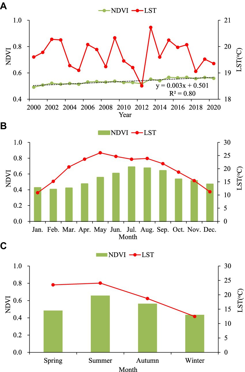
Figure 3. Annual (A), monthly (B) and seasonal (C) changes of NDVI and LST.

From 2002 to 2020, the ranges of average monthly PRCP and ET varied between 74.96 mm to 130.97 mm and 53.63 mm to 64.05 mm, respectively (Figure 4A). Monthly PRCP and ET were primarily concentrated from June to September (Figure 4B). The peak monthly values for PRCP and ET were observed in July, reaching 227.36 mm and 103.97 mm, respectively. In summer, PRCP is the most abundant, while LST and ET achieve their peak levels (Figure 4C).

Figure 4

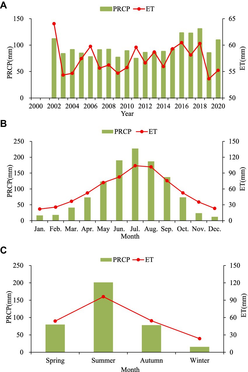
Figure 4. Annual (A), monthly (B) and seasonal (C) changes of PRCP and ET.

3.1.2 NDVI spatial pattern

Spatial distribution of annual average NDVI in the southwestern China displayed significant variability (Figure 5). Most of areas at a low elevation were vegetated, but areas at a high elevation, such as the western Sichuan and northern Tibet were covered by sparse vegetation. Forested regions exhibited the highest NDVI values, predominantly located in southeastern Tibet.

Figure 5

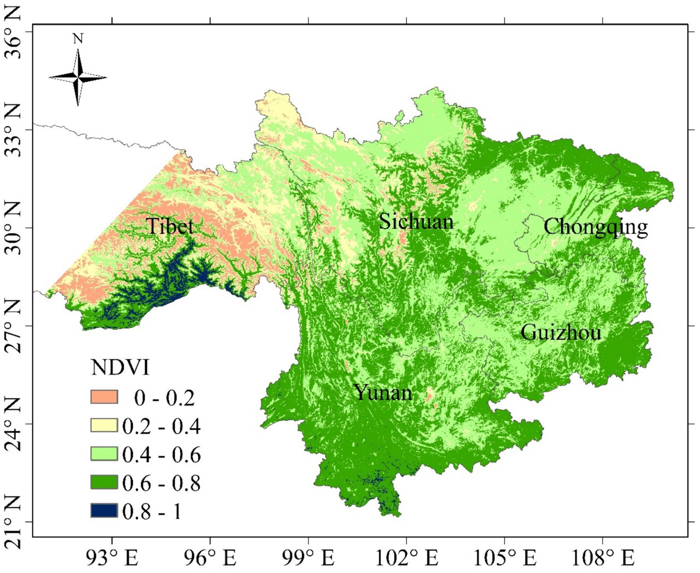
Figure 5. Spatial distribution of annual monthly average NDVI from 2000 to 2020.

3.2 Correlation between vegetation and natural factors

Relationships between NDVI and hydro-climatic variables each month were analyzed via calculating the Spearman’s rank correlation coefficient at a significant level of p < 0.05. According to Figure 6, almost all coefficients were statistically significant at a level of p < 0.05. NDVI had a significant negative correlation with Elv with the r ranging from −0.55 to −0.32, and a positive correlation with Lon, LST and ET, with r ranging from 0.08–0.48, 0.05–0.46 and 0.16–0.61, respectively. NDVI was significantly inversely associated with Lat except in June and July, and with Rs from March to November. Moreover, NDVI had different correlations with Slope, PRCP, Qs, Qsb and TWSC each month.

Figure 6

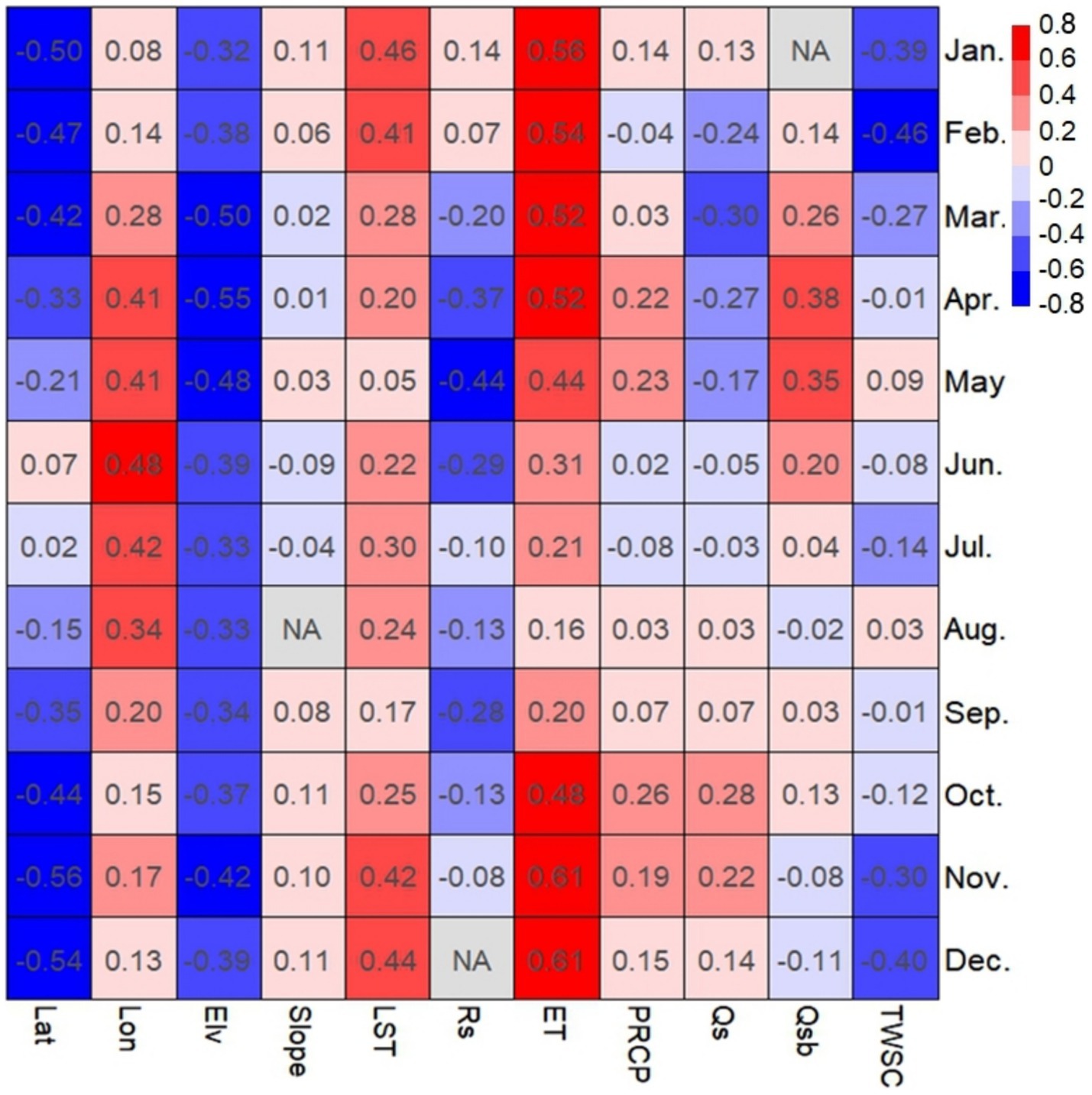
Figure 6. Correlation coefficients between NDVI and natural factors each month (the NA values are not statistically significant at a level of p < 0.05).

The study area was categorized into three regions based on elevation: low, middle, and high. Correlations between vegetation and natural factors varied across different elevations (Table 2). NDVI had a positive correlation with Elv in low-elevation regions, such as the Sichuan Basin, but a negative correlation in the Qinghai Tibet Plateau at high elevations. Besides, NDVI had a stronger positive correlation with Slope, Rs, ET, PRCP and Qs at lower elevations. Correlations between NDVI and Rs were calculated monthly across different elevations. The results presented in Table 3 showed that these correlations were almost universally significant and positive at elevations below 3,000 m.

Table 2

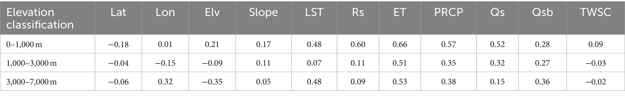
Table 2. Correlation coefficients between NDVI and natural factors in different elevations.

Table 3

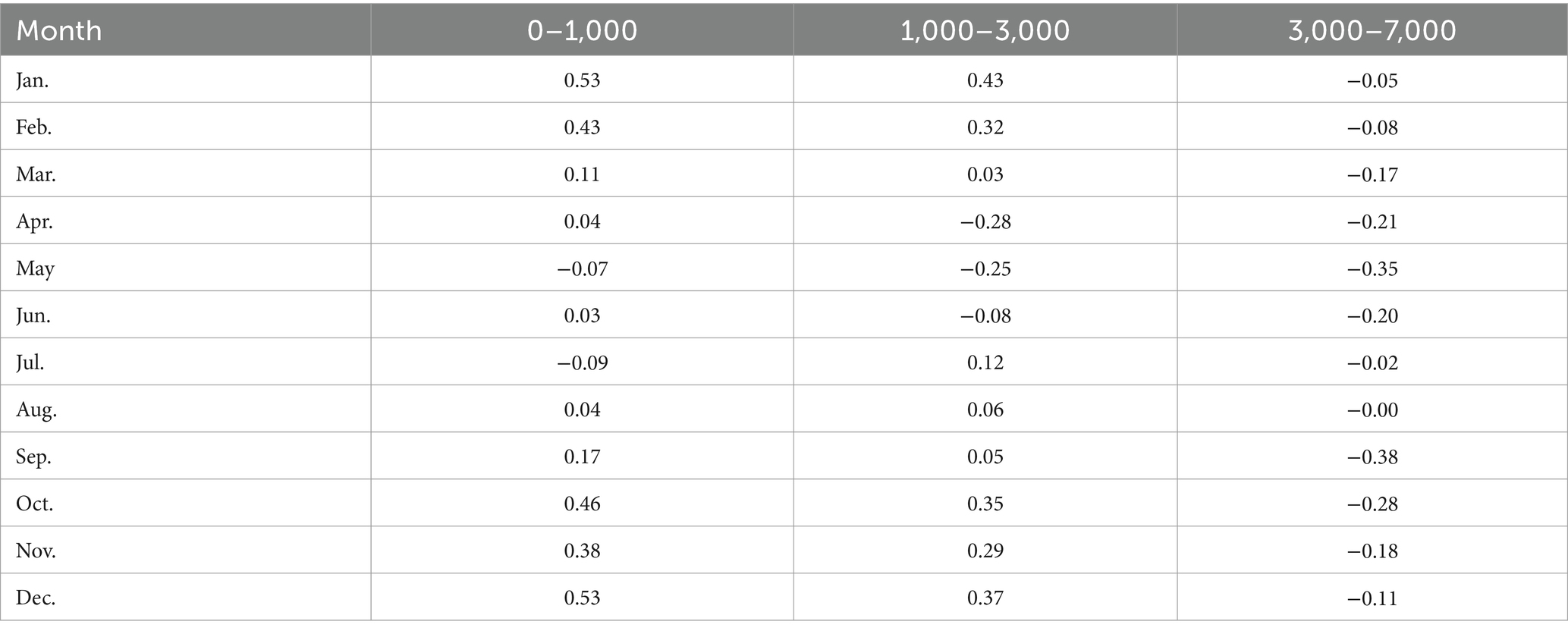
Table 3. Correlation coefficients between NDVI and surface solar radiation in different elevations each month.

3.3 Evaluation of relational models

3.3.1 Construction of relational models

The RF models and the CNN-LSTM models were repeatedly operated with different variables. The initial RF model (RF1) was built with 11 variables from 2002 to 2020 as inputs and had a good predictive precision with R² = 0.83, RMSE = 0.10, RRMSE = 18.16% and MAE = 0.07 (Table 4). Based on the RF1, relative importance of these variables was primarily quantified (Figure 7) and critical variables with higher %IncMSE were used to train new models. These models (RF2 – RF10) adopted different variables as inputs, and accuracy of them generally showed a decreasing trend with the reduction of several key feature variables. Among them, the RF3 achieved the highest precision (R² = 0.83, RMSE = 0.10, RRMSE = 18.08% and MAE = 0.07) while eliminating unimportant variables (Qs, Qsb and TWSC), resulting in an optimize combination of feature variables. The RF10 neglected topographical factors and had the worst performance with the lowest R² of 0.59 and the highest RRMSE of 27.72%.

Table 4

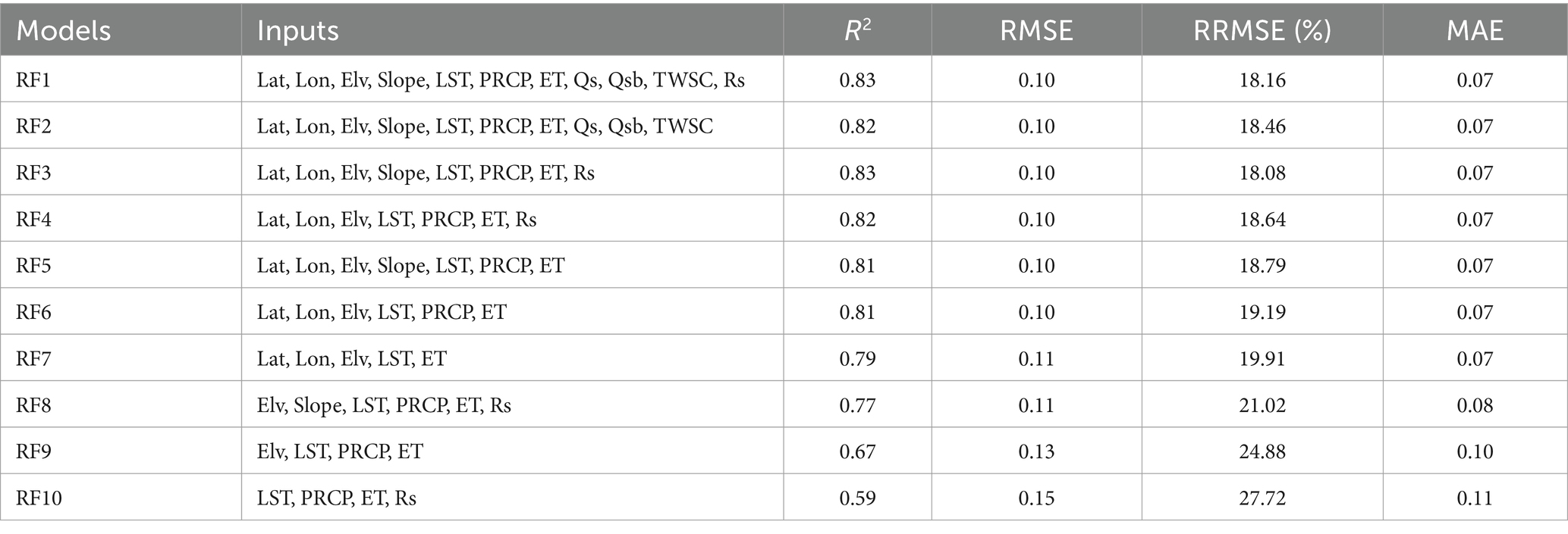
Table 4. Determination coefficient (R²), root mean square error (RMSE), relative root mean square error (RRMSE) and mean absolute error (MAE) for validation of RF models.

Figure 7

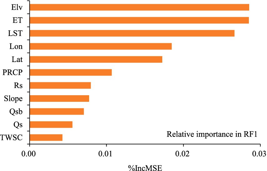
Figure 7. Plots of %IncMSE in the initial Random Forest model (RF1).

Consistent with input variables utilized in RF1, RF2, RF3 and RF10, the four CNN-LSTM models were constructed (Table 5). According to precision indicators, the four models with R² < 0.74 were inferior to RF models except RF9 and RF10. Accuracy of four CNN-LSTM models remained almost unchanged with the reduction of variables with R² changing from 0.71–0.73, RMSE from 0.10–0.11 and RRMSE from 18.59–19.37%. Besides, the CNN-LSTM3 with the same inputs to RF3 had a marginally superior performance than the other three models.

Table 5

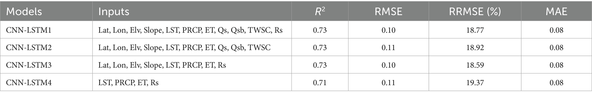
Table 5. Determination coefficient (R²), root mean square error (RMSE), relative root mean square error (RRMSE) and mean absolute error (MAE) for validation of CNN-LSTM models.

3.3.2 Comparison among relational models

The RF3 and CNN-LSTM3, both utilizing identical input variables (Lat, Lon, Elv, Slope, LST, PRCP, ET and Rs) performed, respectively, better than other RF and CNN-LSTM models, and RF3 outperformed CNN-LSTM3 (Tables 4, 5; Figure 8).

Figure 8

Figure 8. Scatter plots between original and predicted NDVI based on the RF3 and CNN-LSTM3 (n_neighbors means the number of neighboring points).

Performance of RF3 and CNN-LSTM3 was further compared on a monthly and seasonal basis, and their precision varied across different months (Table 6). The R² and RRMSE, respectively, changed from 0.60–0.90, 15.20–24.17% for RF3, and 0.43–0.80, 13.50–23.22% for CNN-LSTM3. The estimation precision of RF3 and CNN-LSTM3 was higher in winter and spring.

Table 6

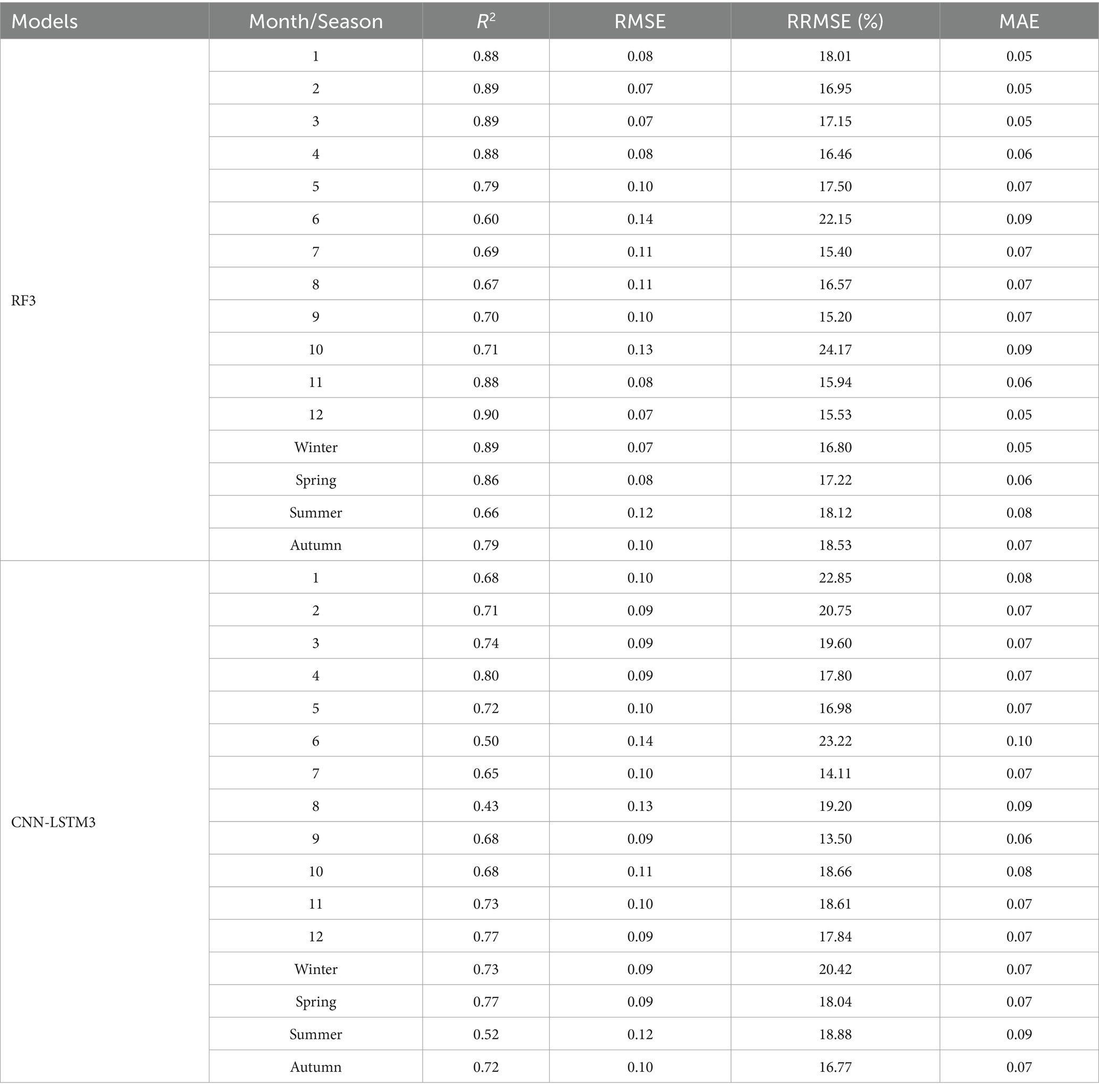
Table 6. Determination coefficient (R²), root mean square error (RMSE), relative root mean square error (RRMSE) and mean absolute error (MAE) of RF3 and CNN-LSTM3 in each month and season.

3.4 Nonlinear relations between vegetation and natural factors

3.4.1 Temporal effects on responses of vegetation to natural factors

The RF3 outperformed all the other models for quantifying relationships between vegetation and natural factors with high dimension data and was extremely sensitive to change of input variables. Therefore, the relative importance (%IncMSE) of 8 natural factors was distinguished by using RF3. Based on the RF3, Elv and LST had more contribution to vegetation growth than other factors (Figures 7, 9).

Figure 9

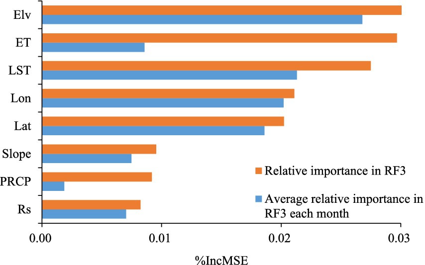
Figure 9. Plot of %IncMSE in RF3 and average %IncMSE in RF3 each month.

Without regard to temporal effects, Elv, ET and LST were primary factors influencing vegetation growth, followed by Lat and Lon. The Slope, PRCP and Rs had a less impact on vegetation. The Qs, Qsb and TWSC were eliminated in the RF3, resulting in lower errors in RF3 than in RF1.

However, temporal scales remarkably affected nonlinear relationships between vegetation and natural factors (Table 6; Figure 9). Climatic factors with seasonal variation characteristics had different effects on vegetation throughout the year. As shown in Figure 9, average monthly %IncMSE values of climatic factors, particularly ET and PRCP, were lower, but the relative importance of terrain factors exhibited less variation across different temporal scales.

3.4.2 Land cover type effects on responses of vegetation to natural factors

Grasslands, forests and croplands were main types of land use in the study area (Figure 2), and their effects on responses of vegetation to natural factors were analyzed. Based on RF3, three local RF models (RF3_forests, RF3_grasses and RF3_croplands) were constructed with 11 variables (Lat, Lon, Elv, Slope, LST, PRCP, ET and Rs) respectively in grasslands, forests and croplands. The simulation accuracy of three local RF models was compared with that of RF3, respectively, in grasslands, forests and croplands. In Table 7, RF3 and three local RF models demonstrated comparable prediction accuracy with R² and RRMSE ranging from 0.71–0.84 and 16.66–18.53%, indicating that the RF models were relatively stable to deal with change of characteristic samples. Among three land cover types, performance of RF models in grasslands was slightly better than in forests and croplands.

Table 7

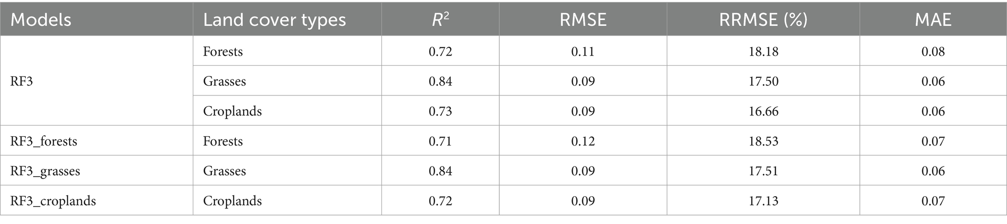
Table 7. Determination coefficient (R²), root mean square error (RMSE), relative root mean square error (RRMSE) and mean absolute error (MAE) of RF3 in different land cover types and 3 local RF models.

Furthermore, relative importance of natural factors in different land cover types was compared. Different determinant factors influenced vegetation growth in forests, grasslands and croplands (Figure 10). LST was dominant factor in forests, while ET and Elv were influential in grasslands, and ET played a significant role in croplands.

Figure 10

Figure 10. Plot of %IncMSE in local RF models in forests, grasslands and croplands.

4 Discussion

4.1 Comparison between RF and CNN-LSTM models

Machine learning is capable of complex tasks, and has a strong advantage in uncovering subtle nonlinear relationships. Thus, the Random Forest and an integration of CNN and LSTM network were used to derive quantitative relationships between NDVI and natural factors and recognize decisive factors, which affected changes of vegetation growth in the mountainous areas. Results showed that RF models outperformed CNN-LSTM models (Tables 4, 5). Compared with CNN-LSTM, RF has more advantages in addressing higher dimensional data, and is more simple and efficient. The out-of-bag error estimate in RF is unbiased, and thus RF is not prone to overfitting (Leo, 2001; Lei et al., 2018). Based on the relative importance of variables, unimportant variables (Qs, Qsb and TWSC) were systematically excluded in the new model (RF3) which yielded higher precision than the original model (RF1). Selecting appropriate topographic and climatic variables as input variables could improve effectively performance of RF models (Chen et al., 2020). RF integrates multiple weak classifiers and adopts the ensemble method to improve its generalization ability. As a result, differences in simulation results of the model (RF3) and three sub-models built with variables, respectively, in grasslands, forests and croplands were not necessarily significant.

Combining the merits of CNN and LSTM, CNN-LSTM has advantages in tasks such as time series prediction. Nevertheless, one-dimensional convolutions in CNN were used in the current paper to traverse topographic and climatic features, and therefore the CNN-LSTM was incapable to handle spatial data effectively. Due to fully connected architecture of LSTM, which provides input-to-state and state-to-state transitions, the CNN-LSTM might be prone to overfitting (Zhao et al., 2021; Liu et al., 2022; Wang et al., 2023).

In addition, spatiotemporal distribution of variables differentially influenced performance of models each month. Estimation precision of RF and CNN-LSTM models was higher from November to May of the following year, but lower from June to October (Table 6). PRCP and ET were concentrated from May and October in the study area, and had seasonal variation characteristics (Figure 4). The seasonality could be a primary factor contributing to the seasonal variations in the performance of relational models.

Influence of topographical factors on performance of RF and CNN-LSTM models was discrepant. Regardless of topographical factors (Lat, Lon, Elv and Slope), simulation accuracy of the RF model (RF10) significantly decreased but that of the CNN-LSTM model (CNN-LSTM4) remained largely unchanged. Due to special structural design in LSTM, LSTM can maintain good performance even in the absence of certain variables (Zhao et al., 2021; Wang et al., 2023). Therefore, RF models have been proven more adept than CNN-LSTM models at quantifying intricate relationships between NDVI and various natural factors in the current study.

4.2 Responses of vegetation to natural factors

The relative importance of eight natural factors was distinguished by using RF3, taking into account temporal effects of features and the influences of various land cover types. Results indicated that elevation, evapotranspiration and temperature were major factors that influenced vegetation growth. Responses of vegetation to major factors, particularly climatic variables, showed slight variations across different periods, suggesting that responses of vegetation toward climatic variables exhibited significant seasonal change (Xu et al., 2018). Besides, there were different decisive factors, which influenced vegetation growth in forests, grasslands and croplands.

Topographic conditions played an indispensable role in interactions between climate changes and vegetation growth in the study area (Chen et al., 2021). Unlike climate variables, the influence of terrain was consistently significant across different periods. Terrain affected the spatial distribution of temperature, precipitation and surface solar radiation, all of which were key factors in determining vegetation distribution. Besides, relationships between vegetation and climatic factors exhibited a spatially and temporally dynamic behavior, and were mainly influenced by topographic conditions (Liu et al., 2018; Zhang et al., 2022). Among topographical factors, elevation had a profound contribution to vegetation growth, and vegetation growth had a significant negative correlation with elevation (Figure 6). Within the study area, low-altitude regions are characterized by a richer distribution of vegetation, attributed to favourable temperature and abundant moisture. In contrast, a significant negative correlation was observed between the aboveground biomass of herbaceous marsh vegetation and altitude in areas at a higher elevation, such as Tibetan Plateau (Shen et al., 2021).

Temperature had a strong positive correlation with NDVI, and significantly influenced vegetation growth, consistent with results from previous studies (Muir et al., 2021; Yang H. et al., 2022; Lai et al., 2023). Vegetation phenology and physiological metabolism were inseparable from temperature changes, and increase in temperature could enhance plant photosynthesis and water utilization efficiency, promoting vegetation growth (Cui et al., 2022; Lai et al., 2023). In the study area, forests are mainly distributed in regions with low altitude and abundant precipitation. In conditions of ample precipitation, temperature emerges as the primary environmental factor influencing the growth of forest vegetation.

Compared to temperature, vegetation was less affected by precipitation in the study area (Cui et al., 2022; Ma et al., 2022), and the effects of precipitation on vegetation varied in each season (Georganos et al., 2017). Weaker correlations between vegetation and precipitation were observed during autumn and winter (Figure 6), aligning with conclusions of previous studies (Worku et al., 2023). Vegetation had a high correlation with rainfall in semi-arid zones and a weaker response in sub-humid and humid climates (Camberlin et al., 2007; Li et al., 2013; Wang et al., 2021). In most of the study area, precipitation was relatively abundant particularly in summer. Excessive precipitation could result in insufficient oxygen supply in the soil and impaired nutrient absorption in the rhizosphere, thereby constraining vegetation growth (Gong et al., 2021; Ma et al., 2022). However, in some ecologically vulnerable areas covered with sparse vegetation, precipitation played a crucial role in vegetation change and had a greater impact on vegetation dynamics compared to temperature (Zhao et al., 2020; Zhang et al., 2021, 2022).

There is a close interrelationship between evapotranspiration and vegetation, and both of them play an essential role in the terrestrial water cycle (Xu et al., 2018; Bai et al., 2020). Vegetation transpiration is an important part of terrestrial evapotranspiration, and evapotranspiration helps regulate the temperature and moisture of vegetation, maintaining the water balance within plants. As a key factor in vegetation growth, evapotranspiration is related to the growth condition of vegetation and closely linked with environmental conditions, climate change, agricultural management, and ecosystem health. Climate change affected evapotranspiration and interrelationships between evapotranspiration and vegetation (Yang H. et al., 2022; Yang L. et al., 2022). Temperature and precipitation were the dominant causes for evaporation changes in China, which affected vegetation growth (Zheng et al., 2022).

Surface solar radiation had a smaller effect on vegetation compared with elevation, temperature and evapotranspiration in the current study. The relationships between vegetation and solar radiation were affected by altitude and temporal factors. NDVI was positively related to surface solar radiation in low-elevation regions (Table 2), which aligns with previous researches (Lai et al., 2023). Solar radiation is important for vegetation photosynthesis, and an appropriate increase in solar radiation can promote vegetation growth. Correlations between NDVI and surface solar radiation were significantly positive at elevations below 3,000 m. In high-altitude areas, intense solar radiation could rapidly increase temperature and water evaporation, leading to soil drought, which was detrimental to the growth of plants (Lai et al., 2023).

In addition, NDVI from 2000–2020 in the study area slightly increased (Figure 3A), which was consistent with numerous studies (Chen et al., 2021; Zhang et al., 2021; Yang H. et al., 2022; Lai et al., 2023). Their researches indicated a trend of vegetation greening in southwest China over the past two decades, owing to the afforestation and conservation of natural forests. Especially in areas characterized by fragile ecosystems, high topographical complexity and suboptimal soil conditions, notable alterations in NDVI had been observed as a result of ecological restoration projects in recent decades (Yang H. et al., 2022; Lai et al., 2023). Some forestry and ecological projects, such as the protection of natural forest resources and the return of farmland to forest and grassland, have been implemented by the state since the end of the 20th century, and have promoted the growth of vegetation and suppressed soil degradation.

5 Conclusion

The current paper explored interactions between hydro-climatic changes and vegetation growth with Random Forest and integrated CNN and LSTM network in the mountainous southwest China by using multi-source remote sensing data. The main results can be summarized as follows:

1. In the study area, NDVI increased slightly from 2000 to 2020, and average monthly NDVI was higher in the maximum growing season (May to September). The correlation analysis revealed a significant negative association between NDVI and elevation, but positive correlations with longitude, land surface temperature and evapotranspiration. The relationships between NDVI and these natural factors exhibited monthly variation.

2. The RF3 excluded unimportant variables, achieving the highest precision through an optimized combination of feature variables. Simulation accuracy of RF and CNN-LSTM models demonstrated significant variability across different months and seasons. The estimation precision for both models was notably higher from November to May of the subsequent year but decreased from June to October.

3. Based on the optimal model (RF3), elevation and land surface temperature had more contribution to vegetation growth than other factors. Effects of climatic factors, such as evapotranspiration and precipitation, on vegetation were markedly influenced by seasonal fluctuations in these factors. Besides, various determinant factors influenced vegetation growth differently in forests, grasslands, and croplands.

Exploring vegetation growth in response to topographic and climatic factors and quantifying their complex nonlinear relationships can provide a valuable guidance for ecological environment conservation. However, there may be some uncertainty in the current study. In practical applications, remote sensing data can be compromised by various environmental interferences, including clouds, fog, rain and snow, potentially influencing research results. Furthermore, the datasets employed in this study encompass multiple spatial resolutions. The application of interpolation techniques to harmonize these spatial resolutions can also introduce certain uncertainty. The two machine learning methods, RF and CNN-LSTM, demonstrate effectiveness in addressing complex nonlinear problems, but they also have certain limitations, such as inability to completely eliminate overfitting in Random Forest due to noises in data, gradient disappearance or gradient explosion in LSTM models and usually longer training time. Further research will focus on exploring influences of topographic conditions and climate change on vegetation by improving accuracy of datasets and models, and analysing effects of multiple spatial and temporal scales of variables.

Data availability statement

Publicly available datasets were analyzed in this study. This data can be found at: https://disc.gsfc.nasa.gov/datasets/GLDAS_NOAH025_M_2.1/summary, https://ladsweb.modaps.eosdis.nasa.gov/, and https://search.earthdata.nasa.gov/.

Author contributions

HC: Writing – review & editing, Validation, Supervision, Methodology, Conceptualization. WZ: Writing – review & editing. ZH: Writing – original draft, Software, Methodology, Formal analysis, Data curation. YZ: Writing – original draft. WW: Writing – original draft, Data curation. TC: Writing – original draft, Supervision, Conceptualization.

Funding

The author(s) declare financial support was received for the research, authorship, and/or publication of this article. This research was supported by the Scientific Research Fund of Chengdu University of Information Technology (KYTZ202128, KYTZ202129, and KYTZ202133), Sichuan Natural Science Foundation (2022NSFSC1000), and National Natural Science Foundation Youth Fund (42007188).

Conflict of interest

The authors declare that the research was conducted in the absence of any commercial or financial relationships that could be construed as a potential conflict of interest.

Publisher’s note

All claims expressed in this article are solely those of the authors and do not necessarily represent those of their affiliated organizations, or those of the publisher, the editors and the reviewers. Any product that may be evaluated in this article, or claim that may be made by its manufacturer, is not guaranteed or endorsed by the publisher.

Footnotes

1. ^https://doi.org/10.11888/Meteoro.tpdc.271023

References

Bai, P., Liu, X., Zhang, Y., and Liu, C. (2020). Assessing the impacts of vegetation greenness change on evapotranspiration and water yield in China. Water Resour. Res. 56:19. doi: 10.1029/2019WR027019

Crossref Full Text | Google Scholar

Camberlin, P., Martiny, N., Philippon, N., and Richard, Y. (2007). Determinants of the interannual relationships between remote sensed photosynthetic activity and rainfall in tropical Africa. Remote Sens. Environ. 106, 199–216. doi: 10.1016/j.rse.2006.08.009

Crossref Full Text | Google Scholar

Cao, H., Han, L., and Li, L. (2022). A deep learning method for cyanobacterial harmful algae blooms prediction in Taihu Lake, China. Harmful Algae 113:102189. doi: 10.1016/j.hal.2022.102189

PubMed Abstract | Crossref Full Text | Google Scholar

Chen, W., Bai, S., Zhao, H., Han, X., and Li, L. (2021). Spatiotemporal analysis and potential impact factors of vegetation variation in the karst region of Southwest China. Environ. Sci. Pollut. Res. 28, 61258–61273. doi: 10.1007/s11356-021-14988-y

PubMed Abstract | Crossref Full Text | Google Scholar

Chen, H., Liu, H., Chen, X., and Qiao, Y. (2020). Analysis on impacts of hydro-climatic changes and human activities on available water changes in Central Asia. Sci. Total Environ. 737:139779. doi: 10.1016/j.scitotenv.2020.139779

PubMed Abstract | Crossref Full Text | Google Scholar

Chen, H., Liu, X., Ding, C., and Huang, F. (2018). Phenology-based residual trend analysis of MODIS-NDVI time series for assessing human-induced land degradation. Sensors 18:3676. doi: 10.3390/s18113676

PubMed Abstract | Crossref Full Text | Google Scholar

Chen, H., Qiao, Y., and Liu, H. (2022). A random forest method for constructing long-term time series of nighttime light in Central Asia. Remote Sens. Appl. Soc. Environ. 25:100687. doi: 10.1016/j.rsase.2021.100687

Crossref Full Text | Google Scholar

Cui, X., Xu, G., He, X., and Luo, D. (2022). Influences of seasonal soil moisture and temperature on vegetation phenology in the Qilian Mountains. Remote Sens. 14:3645. doi: 10.3390/rs14153645

Crossref Full Text | Google Scholar

Duan, C., Li, J., Chen, Y., Ding, Z., Ma, M., Xie, J., et al. (2022). Spatiotemporal dynamics of terrestrial vegetation and its driver analysis over Southwest China from 1982 to 2015. Remote Sens. 14:2497. doi: 10.3390/rs14102497

Crossref Full Text | Google Scholar

Foody, G. M. (2003). Geographical weighting as a further refinement to regression modelling: an example focused on the NDVI–rainfall relationship. Remote Sens. Environ. 88, 283–293. doi: 10.1016/j.rse.2003.08.004

Crossref Full Text | Google Scholar

Gao, P., Du, W., Lei, Q., Li, J., Zhang, S., and Li, N. (2023). NDVI forecasting model based on the combination of time series decomposition and CNN – LSTM. Water Resour. Manag. 37, 1481–1497. doi: 10.1007/s11269-022-03419-3

Crossref Full Text | Google Scholar

Georganos, S., Abdi, A. M., Tenenbaum, D. E., and Kalogirou, S. (2017). Examining the NDVI-rainfall relationship in the semi-arid Sahel using geographically weighted regression. J. Arid Environ. 146, 64–74. doi: 10.1016/j.jaridenv.2017.06.004

Crossref Full Text | Google Scholar

Gong, X., Du, S., Li, F., and Ding, Y. (2021). Study of mesoscale NDVI prediction models in arid and semiarid regions of China under changing environments. Ecol. Indic. 131:108198. doi: 10.1016/j.ecolind.2021.108198

Crossref Full Text | Google Scholar

Hou, W., Gao, J., Wu, S., and Dai, E. (2015). Interannual variations in growing-season NDVI and its correlation with climate variables in the southwestern karst region of China. Remote Sens. 7, 11105–11124. doi: 10.3390/rs70911105

Crossref Full Text | Google Scholar

Lai, J., Zhao, T., and Qi, S. (2023). Spatiotemporal variation in vegetation and its driving mechanisms in the southwest alpine canyon area of China. Forests 14:2357. doi: 10.3390/f14122357

Crossref Full Text | Google Scholar

Lei, C., Deng, J., Cao, K., Ma, L., Xiao, Y., and Ren, L. (2018). A random forest approach for predicting coal spontaneous combustion. Fuel 223, 63–73. doi: 10.1016/j.fuel.2018.03.005

Crossref Full Text | Google Scholar

Leo, B. (2001). Random forests. Mach. Learn. 45, 5–32. doi: 10.1023/A:1010933404324

Crossref Full Text | Google Scholar

Li, S., Xie, Y., Brown, D. G., Bai, Y., Hua, J., and Judd, K. (2013). Spatial variability of the adaptation of grassland vegetation to climatic change in Inner Mongolia of China. Appl. Geogr. 43, 1–12. doi: 10.1016/j.apgeog.2013.05.008

Crossref Full Text | Google Scholar

Li, P., Zhang, J., and Krebs, P. (2022). Prediction of flow based on a CNN-LSTM combined deep learning approach. Water 14:993. doi: 10.3390/w14060993

Crossref Full Text | Google Scholar

Liu, T., Jin, H., Xie, X., Fang, H., Wei, D., and Li, A. (2022). Bi-LSTM model for time series leaf area index estimation using multiple satellite products. IEEE Geosci. Remote Sens. Lett. 19, 1–5. doi: 10.1109/LGRS.2022.3199765

Crossref Full Text | Google Scholar

Liu, H., Zhang, M., Lin, Z., and Xu, X. (2018). Spatial heterogeneity of the relationship between vegetation dynamics and climate change and their driving forces at multiple time scales in Southwest China. Agric. For. Meteorol. 256-257, 10–21. doi: 10.1016/j.agrformet.2018.02.015

Crossref Full Text | Google Scholar

Ma, Y., Guan, Q., Sun, Y., Zhang, J., Yang, L., Yang, E., et al. (2022). Three-dimensional dynamic characteristics of vegetation and its response to climatic factors in the Qilian Mountains. Catena 208:105694. doi: 10.1016/j.catena.2021.105694

Crossref Full Text | Google Scholar

Ma, H., and Liang, S. (2022). Development of the GLASS 250-m leaf area index product (version 6) from MODIS data using the bidirectional LSTM deep learning model. Remote Sens. Environ. 273:112985. doi: 10.1016/j.rse.2022.112985

Crossref Full Text | Google Scholar

Moghim, S. (2020). Assessment of water storage changes using GRACE and GLDAS. Water Resour. Manag. 34, 685–697. doi: 10.1007/s11269-019-02468-5

Crossref Full Text | Google Scholar

Muir, C., Southworth, J., Khatami, R., Herrero, H., and Akyapı, B. (2021). Vegetation dynamics and climatological drivers in Ethiopia at the turn of the century. Remote Sens. 13:3267. doi: 10.3390/rs13163267

Crossref Full Text | Google Scholar

Piao, S., Wang, X., Park, T., Chen, C., Lian, X., He, Y., et al. (2020). Characteristics, drivers and feedbacks of global greening. Nat. Rev. Earth Environ. 1, 14–27. doi: 10.1038/s43017-019-0001-x

Crossref Full Text | Google Scholar

Shen, X., Jiang, M., Lu, X., Liu, X., Liu, B., Zhang, J., et al. (2021). Aboveground biomass and its spatial distribution pattern of herbaceous marsh vegetation in China. Sci. China Earth Sci. 64, 1115–1125. doi: 10.1007/s11430-020-9778-7

Crossref Full Text | Google Scholar

Wang, Y., Shen, X., Jiang, M., Tong, S., and Lu, X. (2021). Spatiotemporal change of aboveground biomass and its response to climate change in marshes of the Tibetan plateau. Int. J. Appl. Earth Obs. Geoinf. 102:102385. doi: 10.1016/j.jag.2021.102385

Crossref Full Text | Google Scholar

Wang, Z., Song, D., He, T., Lu, J., Wang, C., and Zhong, D. (2023). Developing spatial and temporal continuous fractional vegetation cover based on Landsat and Sentinel-2 data with a deep learning approach. Remote Sens. 15:2948. doi: 10.3390/rs15112948

Crossref Full Text | Google Scholar

Worku, M. A., Feyisa, G. L., Beketie, K. T., and Garbolino, E. (2023). Spatiotemporal dynamics of vegetation in response to climate variability in the Borana rangelands of southern Ethiopia. Front. Earth Sci. 11:991176. doi: 10.3389/feart.2023.991176

Crossref Full Text | Google Scholar

Xu, S., Yu, Z., Yang, C., Ji, X., and Zhang, K. (2018). Trends in evapotranspiration and their responses to climate change and vegetation greening over the upper reaches of the Yellow River Basin. Agric. For. Meteorol. 263, 118–129. doi: 10.1016/j.agrformet.2018.08.010

Crossref Full Text | Google Scholar

Yang, L., Feng, Q., Zhu, M., Wang, L., Alizadeh, M. R., Adamowski, J. F., et al. (2022). Variation in actual evapotranspiration and its ties to climate change and vegetation dynamics in Northwest China. J. Hydrol. 607:127533. doi: 10.1016/j.jhydrol.2022.127533

Crossref Full Text | Google Scholar

Yang, H., Hu, J., Zhang, S., Xiong, L., and Xu, Y. (2022). Climate variations vs. human activities: distinguishing the relative roles on vegetation dynamics in the three karst provinces of Southwest China. Front. Earth Sci. 10:799493. doi: 10.3389/feart.2022.799493

Crossref Full Text | Google Scholar

Yin, L., Dai, E., Zheng, D., Wang, Y., Ma, L., and Tong, M. (2020). What drives the vegetation dynamics in the Hengduan Mountain region, Southwest China: climate change or human activity? Ecol. Indic. 112:106013. doi: 10.1016/j.ecolind.2019.106013

Crossref Full Text | Google Scholar

Zafar, Z., Sajid Mehmood, M., Shiyan, Z., Zubair, M., Sajjad, M., and Yaochen, Q. (2023). Fostering deep learning approaches to evaluate the impact of urbanization on vegetation and future prospects. Ecol. Indic. 146:109788. doi: 10.1016/j.ecolind.2022.109788

Crossref Full Text | Google Scholar

Zhang, Y., Liu, Q., Wang, Y., and Huang, J. (2022). Assessing the impacts of climate change and anthropogenic activities on vegetation in Southwest China. J. Mt. Sci. 19, 2678–2692. doi: 10.1007/s11629-021-6984-z

Crossref Full Text | Google Scholar

Zhang, X., Yue, Y., Tong, X., Wang, K., Qi, X., Deng, C., et al. (2021). Eco-engineering controls vegetation trends in Southwest China karst. Sci. Total Environ. 770:145160. doi: 10.1016/j.scitotenv.2021.145160

PubMed Abstract | Crossref Full Text | Google Scholar

Zhao, S., Pereira, P., Wu, X., Zhou, J., Cao, J., and Zhang, W. (2020). Global karst vegetation regime and its response to climate change and human activities. Ecol. Indic. 113:106208. doi: 10.1016/j.ecolind.2020.106208

Crossref Full Text | Google Scholar

Zhao, F., Yang, G., Yang, H., Zhu, Y., Meng, Y., Han, S., et al. (2021). Short and medium-term prediction of winter wheat NDVI based on the DTW–LSTM combination method and MODIS time series data. Remote Sens. 13:4660. doi: 10.3390/rs13224660

Crossref Full Text | Google Scholar

Zheng, H., Miao, C., Li, X., Kong, D., Gou, J., Wu, J., et al. (2022). Effects of vegetation changes and multiple environmental factors on evapotranspiration across China over the past 34 years. Earth's. Future 10:e2021EF002564. doi: 10.1029/2021EF002564

Crossref Full Text | Google Scholar