 Liang Hong
 Mengxi Wang1
 Liyong Fu
- 1Research Institute of Forest Resource Information Techniques, Chinese Academy of Forestry, Beijing, China
- 2School of Mathematics and Statistics, Xinyang Normal University, Xinyang, Henan, China
- 3School of Landscape Architecture, Beijing Forestry University, Beijing, China
Introduction: Crown width (CW) is a significant variable of tree growth, but measuring crown width is laborious and time-consuming. Diameter at breast height (D) is a commonly used growth variable in crown width prediction. Here, a CW-D model was developed to estimate the crown width of larch.
Methods: The data of 1,515 larch trees were collected in Guandi mountain, the northern China. We chose linear function, quadratic function, and other form of base functions to develop the CW models, and we introduced non-linear least squares techniques (NLS), non-linear mixed-effect (NLME), and Bayesian method in modeling process. Because the data was from different plot, we added a plot level random effect in NLME method to predict the effect from environment. For equally comparing the Bayesian method with the NLME, we also added the plot level random effect to the Bayesian MCMC procedure. We selected Akaike's information criterion and logarithm likelihood to evaluate NLS and NLME models, and chose deviance information criterion and stationary test to test Bayesian method. These methods had another three same indicators (the determination coefficient, root mean square error, and mean absolute deviation) in model evaluation.
Results and discussion: Heteroskedasticity wasn't occurred in this study. The model I.2 (quadratic formula) showed a best fitting effect in each method, and Bayesian method with random effect was slightly superior than other methods. Therefore, the selected final model was quadratic function by Bayesian method with plot level random effect, this combination had the highest prediction accuracy in the larch trees' crown width estimation of Guandi mountain.
1 Introduction
Crown width (CW) is one of the important tree variables that is often used to infer tree vigor (Sattler and Lemay, 2011; Fu et al., 2013). Crown width usually indicates the crown shape, crown size, and crown ratio of a tree and reflects the competitiveness of a tree and that of those around it (Hamilton, 1969; Holdaway, 1986; Hasenauer and Monserud, 1996; Baldwin and Peterson, 1997; Purves et al., 2007). Crown width enables to predict tree growth and aboveground biomass, and it can also reflect the forest age, forest density, and the health degree of a forest (Gering and May, 1995; O'Brien et al., 1995; Gill et al., 2000; Gilmore, 2001; Bernetti et al., 2004; Zarnoch et al., 2004; Tahvanainen and Forss, 2008; Paulo and Tomé, 2009; Sönmez, 2009). Many researchers have described the advantages and effects of crown biomass in the forest. Crown width has extensive applications, but measuring the CW of every sampled tree is costly and time-consuming (Bragg, 2001; Condés and Sterba, 2005; Kalliovirta and Tokola, 2005; Sharma et al., 2016). Therefore, many researchers aimed to estimate the crown width according to the relationship between crown width and tree growth (Gering and May, 1995; Monserud and Marshall, 1999; Gill et al., 2000; Gilmore, 2001).
To estimate crown width, researchers often use models that rely on key variables such as height, height-diameter ratio, and diameter at breast height. Among these, diameter at breast height is the most commonly used factor (Gering and May, 1995; Sharma et al., 2016). A simple and common way to predict crown width is by building a model that mainly uses diameter at breast height as a predictor variable (Bechtold, 2003; Fu et al., 2013, 2017b). Significant relationships between crown width and stem diameter have been well-established for many species of trees. Simple linear relationships, quadratic expressions, and other forms of functions between crown width and stem diameter have been developed by many researchers, and these models are usually estimated using ordinary least squares techniques (NLS) (Bechtold, 2003; Sedmák and Scheer, 2012; Fu et al., 2013). However, the crown width is not only related to the tree growth but also connected with the environment around the tree. For example, climatic conditions, site conditions, and density of the stand can affect crown width to different degrees. Observations from the same plot are likely to be significantly correlated, while the environment will influence the independence between observations. Consequently, for accurately estimating the crown width, the plot level effects as a random effect should be taken into consideration (Fu et al., 2013).
A solution to the aforementioned problem is to use a nonlinear mixed-effect (NLME) modeling approach (Fu et al., 2017a,c; Duan et al., 2022). Because the NLME method can explain the fixed and random effects simultaneously, it can provide an efficient means to make accurate local predictions. In recent years, it has become increasingly applied to forest growth and yield modeling. The fixed-effects parameters in NLME models express the same meanings as in general regression, and the random-effects parameters can explain the randomness caused by random factors. The NLME method may have better predictive accuracy than the NLS method, and some research studies supported this conclusion (Fu et al., 2013; Chen et al., 2021; Guo et al., 2023). Therefore, comparing the NLME method with the NLS method in terms of fitting ability is meaningful, especially for crown width estimation.
The NLS and NLME methods are regarded as the classical methods in parameter estimation. The Bayesian model is the other method to efficiently describe complex data and evaluate the uncertainty in parameters (Zhang et al., 2015). The basic difference between the NLS and Bayesian statistics is a different understanding of the probability concept (D'Agostini, 2003; Sedmák and Scheer, 2012). In Bayesian estimation, the prior distribution of probabilities of possible parameter values of the model with the previously defined hyperparameters is combined, and new objective information is included in the measured data of a particular experiment (Sedmák and Scheer, 2012).
In recent years, the Bayesian method has been introduced to estimate parameters for tree growth and yield models (Zhang et al., 2013, 2014; Wang et al., 2019). Zapata-Cuartas et al. (2012) introduced the Bayesian method to estimate tree biomass with high precision. Zhang et al. (2015) used the Bayesian method to estimate the self-thinning line. A Comparison between the classical method and the Bayesian method is also found in some studies, most of which show that the Bayesian method has a slightly better fitting than the classical method (Zell et al., 2014; Zianis et al., 2016; Wang et al., 2019). Some studies also found no significant differences between the mixed model and the Bayesian hierarchical model (Chen et al., 2017).
However, most of these studies only compared the NLS with the Bayesian method, and no random effects were added to the models. Wang et al. (2019) compared the Bayesian method with the NLME method to ensure that all models were compared at the same level; all models had the plot level random effect added in the same position in the NLME and Bayesian methods. The result showed that the Bayesian method was slightly superior to NLME, especially in a small sample size. The systematic comparison of these methods needs further study.
Therefore, this study aims to systematically compare four methods in modeling (NLS, NLME, Bayesian, and Bayesian with random effect) and seeks to determine the magnitude of the differences among them. First, six selected CW-diameter base models were fitted independently to the full sample data using four methods. Several indicators of these base models were calculated for the best model selection in each method, and four superior models were identified. Second, we compared these four models, representing four modeling methods, to determine the best CW model and the best modeling method for 1,515 larch trees.
2 Materials and methods
2.1 Data
The experimental area was located at Guandi Mountain, Jiaocheng County, Shanxi Province, northern China (Figure 1). The growth data of 1,515 Prince Rupprecht larch trees were collected from 25 permanent sample plots (PSP), which were established in the natural stands of the Guandi Mountain forest. The 25 PSPs, each with a square shape, were established in 2015. Guandi Mountain is one of the most important regions where Prince Rupprecht larch is prevalent in China (Fu et al., 2017b). The selected natural PSPs provided representative information on various stand structures, densities, and dominant heights (Table 1). Data collection was undertaken by the Research Institute of Forest Resources Information Techniques, The Chinese Academy of Forestry.
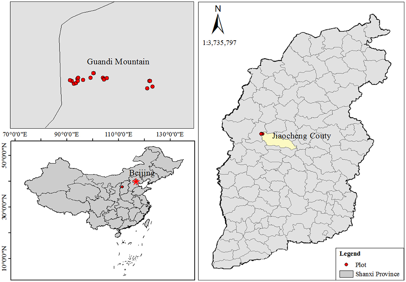
Figure 1. The experimental area, Guandi Mountain, Jiaocheng County, in the Shanxi Province. The red point denotes sample plots, and Shanxi province was described using a black border line and gray base.
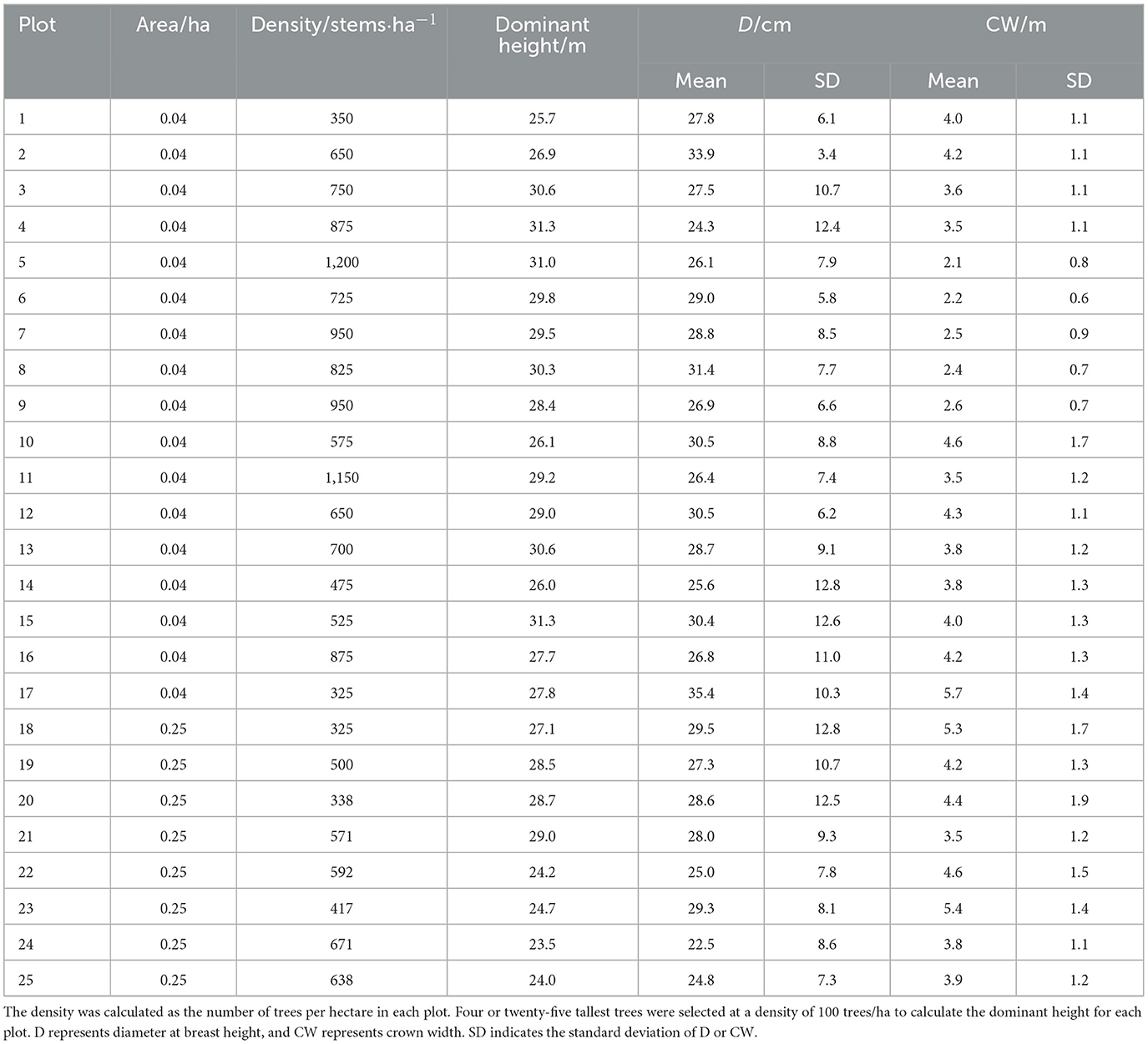
Table 1. Summary of stand factors of the study plots.
Crown width and diameter at breast height of all standing trees with diameter at breast height of ≥3 cm were measured in all 25 PSPs. Crown width was calculated as the half-sum of the four crown radii. The four crown radii were measured as the horizontal distances extending from the center of the tree trunk to the outermost extent of the crown in four cardinal directions (North, South, East, and West) using a laser rangefinder and a compass. A summary statistics of the stand factors of the study plots are presented in Table 1. The relationship between CW and D of all 1,515 larch trees is shown in Figure 2. The nonlinear mixed effects models were constructed using R-3.5.1, and the Bayesian models were run through the MCMC procedure in SAS Institute, Inc (2011).
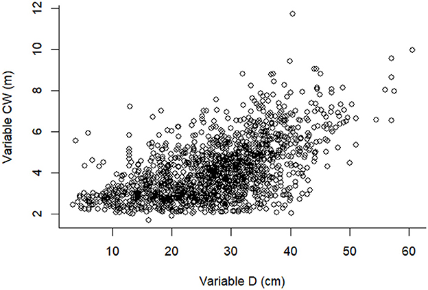
Figure 2. The scatter plot of CW and D of all 1,515 larch trees.
2.2 Methods
2.2.1 Candidate CW-D models
Six candidate models were chosen to model the relationship between crown width and D for trees (Fu et al., 2013). The simplest model used is the linear model (Model I.1). Additionally, some nonlinear models were used in this study for selecting the best model (Models I.2–I.6). These standard models with their function details and function forms are listed in Table 2. All candidate models except Model I.1 are nonlinear, and all functions except Model I.2 have two formal parameters and Model I.2 has three parameters.

Table 2. CW-D base models considered in the research.
2.2.2 Nonlinear mixed effect model
This study involves only one level hierarchical variable. It is a one-level nonlinear mixed effect model as defined by Pinheiro and Bates (2000), and formulated as follows (Carey, 2001; Tang et al., 2015):
where the indices i and j denote the plot level and observation, respectively. yij is a response value of the jth observation (tree) on the ith group, M is the number of the plot level groups, ni is the number of observations (larch trees) on the ith group, and f (…) is a real-valued and differentiable function of a group-specific parameter vector φij and a covariate xij. β is a p-dimensional vector of fixed effects, and the plot level random effect ui is the independent normally distributed q-dimensional vector with zero mean and respective variance–covariance matrix ψ. Aij and Bij are design matrices. ui and εij are independent. The within-group error is assumed to be normally distributed with zero expectation and a positive-definite variance–covariance structure Ri is generally expressed as a function of the parameter vector λ (Fu et al., 2013):
In this study, the sample plot provides the random effect.
2.2.3 The Bayesian method
This study applies Bayesian statistics as one of the ways to develop a CW-D model by modeling six candidate functions. Bayesian statistics is a method developed based on Bayes' rule, which transforms prior probabilities into posterior probabilities, updating the inference of parameters as evidence starts accumulating.
Zhang et al. (2013, 2014) presented Bayes' rule in detail. Let y = (y1, y2,..., yn) represent a vector of data and θ = (θ1, θ2,..., θn) be a vector of parameters to be estimated. Bayes' expression is given as follows:
where p(θ) is the prior distribution for the parameters, and p(θ|y) is the posterior distribution of the Bayesian frameworks.
This study applies the Bayesian method to build crown width models, obtain prior distributions of parameters, and finally achieve posterior distributions. The initial prior information comes from the parameter estimation of NLME. The prior information is adjusted continuously to reach convergence based on the initial prior distribution. All the Bayesian processes were performed in SAS by using the MCMC process. For every Bayesian estimation process, a burn-in period of 10,000 steps and 100,000 iterations were used to estimate parameters. The thinning parameter was set to 5 to reduce the correlation between neighboring iterations (Wang et al., 2019).
2.2.4 Model selection
For testing the goodness-of-fit of six functions, several indicators were calculated. The best functions of the NLS and NLME methods were selected by Akaike's information criterion (AIC) and log-likelihood (Loglik). In contrast, the deviance information criterion (DIC) and stationary test were used for Bayesian model selection. All methods calculated the determination coefficient (R2), mean absolute deviation (MAD), and root mean square error (RMSE) at the same time for the best model selection and different methods of comparison. These indicators are introduced in detail as follows:
where represents the posterior mean of the deviance, is the effective number of parameters in the model, and DIC represents the complexity of the model. A smaller value of DIC for a model indicates a better fit to the data.
The stationary test is a random statistical process that tests whether candidate models are converged. When a model reaches convergence, it means that it has passed the stationary test.
where y is the observed tree crown width, „y is the predicted tree crown width, ȳ is the mean value of the observed tree crown width, and n is the number of individual trees. RMSE combines mean bias and bias variance to provide a robust measure of the overall model accuracy, where is the mean bias and is the bias variance (Fu et al., 2017b). A higher R2 and lower value of RMSE and MAD indicate a good model performance.
3 Results
3.1 NLS CW models
Several fitting indicators of six base functions are presented in Table 3. According to these indicators, these six models had a big difference in fitting. R2 of Models I.4 and I.5 was lower than 0.3, and R2 of the other four models was higher than 0.3. The MAD of Models I.4 and I.5 was lower than 1, while that of the other four models was higher than 1, which indicated that Models I.4 and I.5 were not suited for crown width modeling. Table 3 shows Models I.2 and I.6 presented superior fitting abilities than the other four base models. We compared all the indicators, and Model I.2 (a quadratic form) showed a slightly better predictive ability. Therefore, Model I.2 was selected as the best model for developing the crown width model using the NLS method. The parameters and standard error of this function are listed in Table 4.
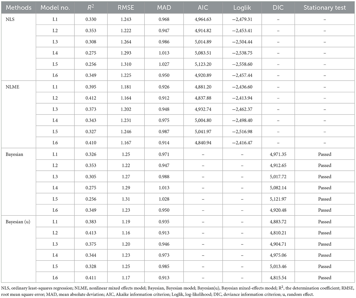
Table 3. Fitting performance of four methods for CW-D base models.
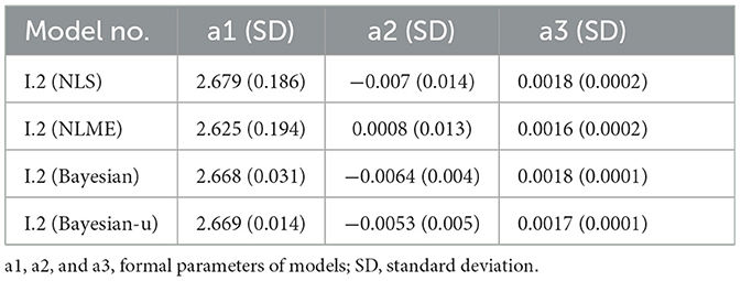
Table 4. Parameters of four best models selected by four methods.
3.2 Bayesian CW models
Table 3 shows the goodness-of-fit of the Bayesian method; all models passed the stationary test and reached convergence. Model I.5 had the lowest R2 (0.256) and the highest RMSE, MAD, and DIC; thus, it was not appropriate for use as a CW model. Model I.2 consistently had the best performance with or without random effect, as it had the lowest DIC value. Therefore, Model I.2 was selected as the best model for the Bayesian method, and the parameters of the function are shown in Table 4.
3.3 Bayesian CW models with random effects at sample plot level
Table 3 also lists the fitting indicators of the Bayesian models with random effects at the sample plot level. All the models passed the stationary test. Compared to the NLS, the R2 of all six models was higher than 0.3, and MAD was lower than 1. Though the predictive ability was approved in all six models, Model I.2 was still the best CW model in this modeling method.
3.4 NLME CW models
The NLME method can explain the general regression and the random effects at the same time. The fitting effects of this method are also listed in Table 3. Compared to the NLS method, all base models had better goodness-of-fit; furthermore, R2 values were higher, while RMSE, MAD, and AIC values were lower than the NLS method. Similar to the three methods discussed, Model I.2 was observed as the best CW model in NLME.
3.5 Models evaluation
In this study, several indicators were used to select the best models among the four methods. The results of each method and each model are listed in Table 3. Table 3 also shows the fitting performance of NLS and NLME. According to these indicators, Model I.2 has the lowest AIC and the highest Loglik for both NLS and NLME and the lowest DIC for the Bayesian method. Thus, Model I.2 is the best model among the four methods. Comparing these four models, we found a significant difference when the plot random effect was added to the model. The R2 of NLME was 16.7% higher than that of NLS, and the RMSE, MAD, AIC, and absolute value of Loglik all decreased than NLS. In addition, the Bayesian method with random effects at the sample plot level was superior to the general Bayesian method, and the R2 showed a 16.9% increase.
According to the results, although evaluation indicators of the NLS and Bayesian methods were almost identical, the Bayesian method was slightly superior to NLS. The same result was obtained when comparing between NLME and Bayesian with random effects at the sample plot level. The parameters of the four models are listed in Table 4. All parameters of the four methods were similar; only a2 in NLME had a different sign. According to the standard deviation, the Bayesian method has a lower standard deviation value than the classical method, proving that the Bayesian method has better stability than the classical method in parameter estimation.
4 Discussion
This study developed a general individual tree CW-D model to estimate the CW of larch. Crown width is an important variable of trees. It is the basis of crown biomass calculation, the crown layer competition measurement, and the tree's age estimation (O'Brien et al., 1995; Bragg, 2001; Purves et al., 2007; Tahvanainen and Forss, 2008). In this study, we compared four different modeling methods and six different base models to choose the best method and the best model for CW estimation. This study also attempted to compare four parameter estimation methods to determine the magnitude of the differences.
The results showed that Model I.2 was the best model and had the best fitting effect among all four methods. In fact, the scatter plot of trees exhibited a quadratic or linear relationship between CW and D, as shown in Figure 2. This finding could be due to a great relationship between the location of the sample plot and tree species (Smith, 1983; Dale et al., 1985). Many researchers have concluded that species and experimental locations should be taken into consideration when developing tree growth and yield models as there may be a strong correlation between the adaption of different species and different areas. Therefore, we need to use a regional model to calculate biomass and tree height or develop a new specific model tailored to specific tree species and locations. From the results of the four methods (Table 3), we observed that although the different methods had minor variations in parameter values, the order of fitting effects in each model remained consistent across all methods. This conclusion also establishes that there is an appropriate difference in each model, and this difference is similar across all methods.
The difference in the area not only affected the base model selection but also had effects on parameter estimation, and therefore, NLME models were introduced. We also added the random effect into each base model. This aid us in dealing with the hierarchical data structure because observations were from different sample plots (Li et al., 2011; Xu et al., 2014; Fu et al., 2017b). For a better comparison between the Bayesian method and the NLME method, we added the random effect into Bayesian models when processing the Bayesian method in the SAS MCMC procedure, which was used to compare these two methods at the same level. In this study, our data was from only one area, Guandi Mountain, thus we decided to develop a one-level NLME model with a plot level random effect added; thus, the effect of different sample plots would be predicted.
After determining the random effect, we need to choose where to place the random effect in the models. This study tested this question. Regarding AIC and Loglik as indicators, we placed the plot level random effect in any combination of the models' parameters (for example, models with two parameters exist in three combinations—a1/a2/a1a2). A lower AIC and higher Loglik indicated better goodness of fit. The results of the NLME models are listed in Table 5. It reveals a trend that the more parameters the random effect added, the better the fitting effect would be, with the exception of Model I.6. This trend might be because the plot level random effect has effects on each parameter, although the significant and partial effects were different. In short, the effect of random effect was not fixed on one specific parameter, and it might work on any parameter.
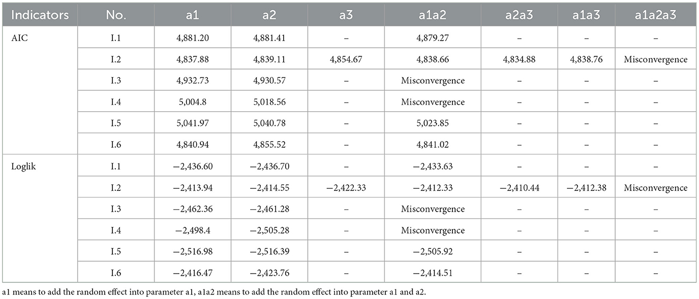
Table 5. The AIC and Loglik of NLME models.
Another conclusion indicated that if the random effect was added in all parameters, the model found it hard to reach convergence. In our study, Models I.2, I.3, and I.4 showed the mentioned problem; when we added the random effect to all parameters, these models did not reach convergence. Even in the Bayesian MCMC processing (SAS), when random effects were added to two or more parameters, this convergence problem occurred. Therefore, to ensure all models and methods are compared at the same level, and all models can reach convergence, we added the plot level random effect only in parameter a1; consequently our comparison of methods is justified.
The results of the comparison showed that the Bayesian method with plot random effect had a better fitness effect than the other three methods. A similar comparison was made in previous studies (Zapata-Cuartas et al., 2012; Wang et al., 2019). Wang et al. (2019) proved that the Bayesian method was slightly superior to the classical method (NLS, NLME), and the estimated results of the parameters showed that the Bayesian method was more stable. From Tables 3, 4, we obtained the same results; the predicted results of parameters and indicators showed that the Bayesian method was superior and stable. In addition, we can also conclude that the Bayesian method has a good fitting effect when the sample data is small (Wang et al., 2019). Zapata-Cuartas et al. (2012) compared different sample data sizes and concluded that the Bayesian method is better than the least-square regression in small sample sizes. Wang et al. (2019) made the same comparison and showed that the Bayesian method was more appropriate for estimating aboveground biomass when the sample size was small. Due to spatial constraints and the identified main focus of this study, we did not compare different sample sizes, but we will attempt it in future research.
In some studies, a heteroscedasticity problem often occurs in preliminary analysis. Heteroscedasticity means the residuals of models obviously tended to increase or decrease as the predicted values increased (Fu et al., 2017b). Several functions applied to a variable account for heteroscedasticity, and the exponential variance function is one of the most commonly used. These functions could cause the unusual trend to disappear in modeling processing (Fu et al., 2017c). The residuals of predictions from four superior CW models with or without the plot level random effect are shown in Figure 3, which shows that there was no heteroscedasticity problem in our analyses, and therefore, we did not use those functions in this study.
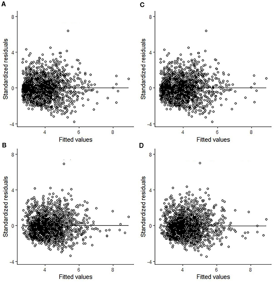
Figure 3. Residuals of best models chosen by four methods (Model I.2). (A) NLS. (B) NLME. (C) Bayesian. (D) Bayesian (u).
The CW models serve as valuable sub-models for tree growth simulators, which are essential for forestry decision-making. The models with random effects enhance prediction accuracy by leveraging limited tree information (Meng and Huang, 2009; Fu et al., 2020). The key lies in selecting sample trees, which must represent the entire population within the sample plot. By estimating the random effect parameters from these selected trees, the models with random effects can capture the inherent variability within the dataset. However, when model users encounter difficulties in localizing the models (NLME and Bayesian with random effect) through the adjustment of sample plot-level random effect parameters, such as ui, which can be estimated using empirical best linear unbiased prediction theory (Pinheiro and Bates, 2000), alternative approaches need to be considered. In such scenarios, NLS may serve as a more practical alternative than the mean response prediction of the models (NLME and Bayesian with random effect) (Sharma and Breidenbach, 2015).
5 Conclusion
A predictive model for determining the crown width of individual larch trees was formulated. Given its significant influence on tree growth, the diameter at breast height was selected as the primary predictor in this model. Model I.2 emerged as the optimal base model for predicting crown width, as all four methods (NLS, NLME, Bayesian, and Bayesian with random effect) concurred on its superiority. Furthermore, the Bayesian model with random effect added in a1 was proven to be the most effective approach in developing the crown width model. Therefore, we recommend utilizing Model I.2 by the Bayesian approach with a random effect for estimating the crown width of Prince Rupprecht larch in northern China.
Data availability statement
The raw data supporting the conclusions of this article will be made available by the authors, without undue reservation.
Author contributions
LH: Data curation, Investigation, Methodology, Supervision, Validation, Writing – original draft. MW: Data curation, Formal analysis, Investigation, Methodology, Writing – original draft. LFe: Data curation, Visualization, Writing – review & editing. GD: Conceptualization, Data curation, Formal analysis, Methodology, Validation, Writing – review & editing. LFu: Data curation, Formal analysis, Methodology, Validation, Writing – review & editing. XW: Conceptualization, Data curation, Formal analysis, Funding acquisition, Investigation, Methodology, Supervision, Validation, Writing – review & editing.
Funding
The author(s) declare financial support was received for the research, authorship, and/or publication of this article. This study was supported by National Natural Science Foundations of China (No. 31971653).
Conflict of interest
The authors declare that the research was conducted in the absence of any commercial or financial relationships that could be construed as a potential conflict of interest.
Publisher's note
All claims expressed in this article are solely those of the authors and do not necessarily represent those of their affiliated organizations, or those of the publisher, the editors and the reviewers. Any product that may be evaluated in this article, or claim that may be made by its manufacturer, is not guaranteed or endorsed by the publisher.
References
Baldwin, V. C. Jr., and Peterson, K. D. (1997). Predicting the crown shape of loblolly pine trees. Can. J. For. Res. 27, 102–107. doi: 10.1139/x96-100
Bechtold, W. A. (2003). Crown-diameter prediction models for 87 species of stand-grown trees in the Eastern United States. South. J. Appl. For. 27, 269–278. doi: 10.1093/sjaf/27.4.269
Bernetti, I., Fagarazzi, C., and Fratini, R. (2004). A methodology to anaylse the potential development of biomass-energy sector: an application in Tuscany. For. Policy Econ. 6, 415–432. doi: 10.1016/j.forpol.2004.03.018
Bragg, D. C. (2001). A local basal area adjustment for crown width prediction. Northern J. Appl. Forestry 18, 22–28. doi: 10.1093/njaf/18.1.22
Carey, V. J. (2001). Mixed-effects models in S and S-Plus by Jose C. Pinheiro; Douglas M. Bates. J. Am. Stat. Assoc. 96, 1135–1136. doi: 10.1198/jasa.2001.s411
Chen, D., Huang, X., Zhang, S., and Sun, X. (2017). Biomass modeling of larch (Larix spp.) plantations in china based on the mixed model, dummy variable model, and Bayesian Hierarchical Model. Forests 8:268. doi: 10.3390/f8080268
Chen, Q., Duan, G., Liu, Q., Ye, Q., Sharma, R. P., Chen, F., et al. (2021). Estimating crown width in degraded forest: a two-level nonlinear mixed-effects crown width model for Dacrydium pierrei and Podocarpus imbricatus in tropical China. For. Ecol. Manage. 497:119486. doi: 10.1016/j.foreco.2021.119486
Condés, S., and Sterba, H. (2005). Derivation of compatible crown width equations for some important tree species of Spain. For. Ecol. Manage. 217, 203–218. doi: 10.1016/j.foreco.2005.06.002
D'Agostini, G. (2003). Bayesian inference in processing experimental data: principles and basic applications. Rep. Prog. Phys. 66, 1383–1419. doi: 10.1088/0034-4885/66/9/201
Dale, V. H., Doyle, T. W., and Shugart, H. H. (1985). A comparison of tree growth models. Ecol. Model. 29, 145–169. doi: 10.1016/0304-3800(85)90051-1
Duan, G., Lei, X., Zhang, X., and Liu, X. (2022). Site index modeling of larch using a mixed-effects model across regional site types in Northern China. Forests 13:815. doi: 10.3390/f13050815
Fu, L., Duan, G., Ye, Q., Meng, X., Luo, P., Sharma, R. P., et al. (2020). Prediction of individual tree diameter using a nonlinear mixed-effects modeling approach and airborne LiDAR data. Remote Sen. 12:1066. doi: 10.3390/rs12071066
Fu, L., Lei, X., Hu, Z., Zeng, W., Tang, S., Marshall, P., et al. (2017a). Integrating regional climate change into allometric equations for estimating tree aboveground biomass of Masson pine in China. Ann. For. Sci. 74:42. doi: 10.1007/s13595-017-0636-z
Fu, L., Sharma, R. P., Hao, K., and Tang, S. (2017b). A generalized interregional nonlinear mixed-effects crown width model for Prince Rupprecht larch in northern China. For. Ecol. Manage. 389, 364–373. doi: 10.1016/j.foreco.2016.12.034
Fu, L., Sun, H., Sharma, R. P., Lei, Y., and Zhang, H. (2013). Nonlinear mixed-effects crown width models for individual trees of Chinese fir (Cunninghamia lanceolata) in south-central China. For. Ecol. Manage. 302, 210–220. doi: 10.1016/j.foreco.2013.03.036
Fu, L., Zhang, H., Sharma, R. P., Pang, L., and Wang, G. (2017c). A generalized nonlinear mixed-effects height to crown base model for Mongolian oak in northeast China. For. Ecol. Manage. 384, 34–43. doi: 10.1016/j.foreco.2016.09.012
Gering, L. R., and May, D. M. (1995). The relationship of diameter at breast height and crown diameter for four species groups in Hardin County, Tennessee. South. J. Appl. For. 19, 177–181. doi: 10.1093/sjaf/19.4.177
Gill, S. J., Biging, G. S., and Murphy, E. C. (2000). Modeling conifer tree crown radius and estimating canopy cover. For. Ecol. Manage. 126, 405–416. doi: 10.1016/S0378-1127(99)00113-9
Gilmore, D. W. (2001). Equations to describe crown allometry of Larix require local validation. For. Ecol. Manage. 148, 109–116. doi: 10.1016/S0378-1127(00)00493-X
Guo, H., Jia, W., Li, D., Sun, Y., Wang, F., Zhang, X., et al. (2023). Modelling branch growth of Korean pine plantations based on stand conditions and climatic factors. For. Ecol. Manage. 546:121318. doi: 10.1016/j.foreco.2023.121318
Hamilton, G. J. (1969). The dependence of volume increment of individual trees on dominance, crown dimensions, and competition. Forestry 8, 133–144. doi: 10.1093/forestry/42.2.133
Hasenauer, H., and Monserud, R. A. (1996). A crown ratio model for Austrian forests. For. Ecol. Manage. 84, 49–60. doi: 10.1016/0378-1127(96)03768-1
Kalliovirta, J., and Tokola, T. (2005). Functions for estimating stem diameter and tree age using tree height, crown width and existing stand database information. Silva Fenn. 39, 227–248. doi: 10.14214/sf.386
Li, Y., Jiang, L., and Liu, M. (2011). A nonlinear mixed-effects model to predict stem cumulative biomass of standing trees. Proc. Environ. Sci. 10, 215–221. doi: 10.1016/j.proenv.2011.09.037
Meng, S. X., and Huang, S. (2009). Improved calibration of nonlinear mixed-effects models demonstrated on a height growth function. For. Sci. 55, 238–248. doi: 10.1093/forestscience/55.3.238
Monserud, R. A., and Marshall, J. D. (1999). Allometric crown relations in three northern Idaho conifer species. Can. J. For. Res. 29, 521–535. doi: 10.1139/x99-015
O'Brien, S. T., Hubbell, S. P., Spiro, P., Condit, R., and Foster, R. B. (1995). Diameter, height, crown, and age relationship in eight neotropical tree species. Ecology 76, 1926–1939. doi: 10.2307/1940724
Paulo, J. A., and Tomé, M. (2009). An individual tree growth model for juvenile cork oak stands in Southern Portugal. Silva Lusit. 1, 27–38.
Pinheiro, J. C., and Bates, D. M. (2000). Mixed-effects Models in S and S-PLUS. New York, NY: Springer. doi: 10.1007/978-1-4419-0318-1
Purves, D. W., Lichstein, J. W., and Pacala, S. W. (2007). Crown plasticity and competition for canopy space: a new spatially implicit model parameterized for 250 North American tree species. PLoS ONE 2:e870. doi: 10.1371/journal.pone.0000870
Sattler, D. F., and Lemay, V. (2011). A system of nonlinear simultaneous equations for crown length and crown radius for the forest dynamics model SORTIE-ND. Can. J. For. Res. 41, 1567–1576. doi: 10.1139/x11-078
Sedmák, R., and Scheer, L. (2012). Modelling of tree diameter growth using growth functions parameterised by least squares and Bayesian methods. J. For. Sci. 58, 245–252. doi: 10.17221/66/2011-JFS
Sharma, R. P., and Breidenbach, J. (2015). Modeling height-diameter relationships for Norway spruce, scots pine, and downy birch using Norwegian national forest inventory data. For. Sci. Technol. 11, 44–53. doi: 10.1080/21580103.2014.957354
Sharma, R. P., Vacek, Z., and Vacek, S. (2016). Individual tree crown width models for Norway spruce and European beech in Czech Republic. For. Ecol. Manage. 366, 208–220. doi: 10.1016/j.foreco.2016.01.040
Smith, W. B. (1983). Adjusting the Stems Regional Forest Growth Model to Improve Local Predictions. Research Note NC-297. St. Paul, MN: U.S. Dept. of Agriculture, Forest Service, North Central Forest Experiment Station. doi: 10.2737/NC-RN-297
Sönmez, T. (2009). Diameter at breast height-crown diameter prediction models for Picea orientalis. Afr. J. Agric. Res. 4, 214–219.
Tahvanainen, T., and Forss, E. (2008). Individual tree models for the crown biomass distribution of Scots pine, Norway spruce and birch in Finland. For. Ecol. Manage. 255, 455–467. doi: 10.1016/j.foreco.2007.09.035
Tang, S., Li, Y., and Fu, L. (2015). Statistical Foundation for Biomathematical Models. Beijing: Higher Education Press.
Wang, M., Liu, Q., Fu, L., Wang, G., and Zhang, X. (2019). Airborne LIDAR-derived aboveground biomass estimates using a hierarchical Bayesian approach. Remote Sens. 11:1050. doi: 10.3390/rs11091050
Xu, H., Sun, Y., Wang, X., Fu, Y., Dong, Y., Li, Y., et al. (2014). Nonlinear mixed-effects (NLME) diameter growth models for individual China-Fir (Cunninghamia lanceolata) trees in Southeast China. PLoS ONE 9:e104012. doi: 10.1371/journal.pone.0104012
Zapata-Cuartas, M., Sierra, C. A., and Alleman, L. (2012). Probability distribution of allometric coefficients and Bayesian estimation of aboveground tree biomass. For. Ecol. Manage. 277, 173–179. doi: 10.1016/j.foreco.2012.04.030
Zarnoch, S. J., Bechtold, W. A., and Stolte, K. W. (2004). Using crown condition variables as indicators of forest health. Can. J. For. Res. 34, 1057–1070. doi: 10.1139/x03-277
Zell, J., Bösch, B., and Kändler, G. (2014). Estimating aboveground biomass of trees: comparing Bayesian calibration with regression technique. Eur. J. For. Res. 133, 649–660. doi: 10.1007/s10342-014-0793-7
Zhang, X., Duan, A., and Zhang, J. (2013). Tree biomass estimation of Chinese fir (Cunninghamia lanceolata) based on Bayesian method. PLoS ONE 8:e79868. doi: 10.1371/journal.pone.0079868
Zhang, X., Duan, A., Zhang, J., and Xiang, C. (2014). Estimating tree height-diameter models with the Bayesian method. Sci. World J. 2014:683691. doi: 10.1155/2014/683691
Zhang, X., Zhang, J., and Duan, A. (2015). A hierarchical bayesian model to predict self-thinning line for Chinese Fir in Southern China. PLoS ONE 10:e0139788. doi: 10.1371/journal.pone.0139788
Keywords: crown width, diameter at breast height, nonlinear least squares, nonlinear mixed-effect, Bayesian method
Citation: Hong L, Wang M, Feng L, Duan G, Fu L and Wang X (2024) The comparison of the Bayesian method with the classical methods in modeling crown width for Prince Rupprecht larch in northern China. Front. For. Glob. Change 7:1405639. doi: 10.3389/ffgc.2024.1405639
Received: 23 March 2024; Accepted: 11 June 2024;
Published: 04 July 2024.
Edited by:
Aldo Rafael Martínez Sifuentes, National Institute of Forestry and Agricultural Research (INIFAP), MexicoReviewed by:
Andressa Ribeiro, Federal University of Piauí, BrazilPetras Rupšys, Vytautas Magnus University, Lithuania
Copyright © 2024 Hong, Wang, Feng, Duan, Fu and Wang. This is an open-access article distributed under the terms of the Creative Commons Attribution License (CC BY). The use, distribution or reproduction in other forums is permitted, provided the original author(s) and the copyright owner(s) are credited and that the original publication in this journal is cited, in accordance with accepted academic practice. No use, distribution or reproduction is permitted which does not comply with these terms.
*Correspondence: Xiyue Wang, d2FuZ3h5NDAyQGJqZnUuZWR1LmNu