 Markku Larjavaara
 Xia Chen2,3*†
 Mingyu Luo
- 1Department of Forest Sciences, University of Helsinki, Helsinki, Finland
- 2Institute of Ecology and Key Laboratory for Earth Surface Processes of the Ministry of Education, College of Urban and Environmental Sciences, Peking University, Beijing, China
- 3State Key Laboratory of Subtropical Silviculture, Zhejiang A&F University, Hangzhou, China
Forests benefit humans in numerous ways. Many of these benefits are greater from forests with large trees and high biomass (i.e., above-ground biomass) than from young forests with small trees. Understanding how the biomass accumulation rate depends on climate is therefore important. According to a classic theory, the biomass accumulation rate first increases until canopy closure, as leaf area and gross primary productivity increase, and decreases thereafter because leaf area cannot increase further and maintaining larger biomass is energetically costlier as living tissue increases even though its proportion of all biomass decreases. We based our modeling on this classic theory and defined relative productivity, pr indicating productivity, and relative maintenance cost, cr, signaling the expense of sustaining a unit of biomass in humid climates of the world. The biomass accumulation rate of low biomass forests is determined by pr − cr and maximal biomass by pr/cr. We then compiled a global data set from the literature, with 3,177 records to fit a parameter for the efficiency of converting surplus carbon into accumulated biomass and another parameter determining biomass at canopy closure. Based on the parameterized models, a constant temperature of 22.3°C leads to the most rapid biomass accumulation in low biomass forests, whereas 16.4°C results in greatest maximal biomass. Our parameterized model can be applied to both climate change adaptation and mitigation by optimizing land use.
1 Introduction
Human-caused deforestation has a long history (Kirch, 2005). Only its magnitude is known for the distant past, and more trustworthy numbers are available only for recent centuries. For example, over 20% of forests of 1700 have been cleared since then (Ramankutty and Foley, 1999; FAO, 2020). Deforestation is problematic as forests are beneficial for humans for numerous reasons that are often called “forest ecosystem services” (Acharya et al., 2019). Several campaigns are therefore working to restore these benefits by afforesting open areas that were previously forestland (Lewis et al., 2019). Many of the benefits provided by forests result from the large size of trees. Trees in young forests are still small and therefore potentially benefit humans less than potentially large trees in old forests. The slow start can cause significant time lags. Understanding how rapidly a new forest will approach the characteristics of an old forest is therefore important, for example, for optimally allocating efforts to reduce the deforestation of old forests relative to establishing new forests, i.e., afforestation.
Several potential tree size-related statistics may be used to indicate the recovery level of a new forest to which the benefits of forests to humans can be linked. Volume and biomass per unit land area are commonly used to let both the number of trees per unit area and their size influence the metric. In plantation forestry mainly aiming to produce timber, trunk volume per unit area is the most common metric (West, 2014). However, when the focus is on forest benefits other than timber or when the perspective is ecological, it is more appropriate to use biomass influenced by wood density and other tree parts rather than solely trunks (Larjavaara, 2021). In practice, because roots are difficult to measure, only above-ground biomass (hereafter “biomass” or “b” as seen in Table 1), is commonly used to describe the development stage of a forest (Anderson-Teixeira et al., 2016).
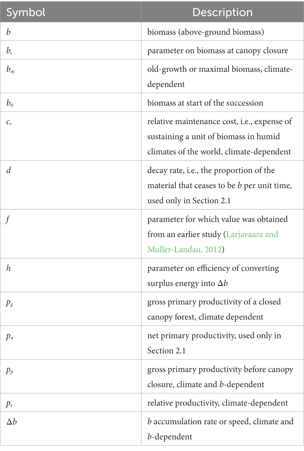
Table 1. List of variables and parameters.
How do benefits of forests to humans depend on b in a successional forest? Climate change mitigation is the simplest case, as approximately half of tree biomass is carbon (Martin and Thomas, 2011) that, if not locked in wood and other tree tissues, can be assumed to be fully or proportionally in the atmosphere as carbon dioxide. Therefore, doubling b doubles the climate benefit when complications, such as carbon in the roots or wood products, their substitution impacts (Hurmekoski et al., 2021), or non-carbon-related climate impacts of forests, such as those related to methane (Pangala et al., 2017) or albedo (Kuusinen et al., 2012), are not considered. Another perspective is needed when focusing on another important forest benefit, timber yield, as there is no value without harvesting. The value of harvested timber in a clear-cut depends strongly on b, as it correlates well to trunk volume per unit area (Penman et al., 2003). However, the cost of harvesting per unit of timber decreases with b (Adebayo et al., 2007), and the proportion of trunks of b (Wang, 2006) and the proportion of high-quality wood in trunks both increase with increasing b (Kolis et al., 2014). Therefore, the net value of timber per unit forest area increases much faster than proportionally to b (Kolis et al., 2014). Non-timber forest products are highly diverse and include examples of both positive and negative correlations with b. For example, a certain berry-yielding Vaccinium sp. increases with forest age and b in Finland (Miina et al., 2009), while another decreases (Turtiainen et al., 2016). Another way in which forests can benefit humans is by reducing erosion and the risk of landslides and floods. Canopy cover or leaf area per unit area matter hydrologically and for controlling erosion, and relatively young forests with small b but already closed canopy, may be as effective as older ones (Sidle et al., 2006; Ellison et al., 2017). However, a deep coarse root system developing slowly with increasing b may be significant in preventing landslides (Sidle et al., 2006). Forest value for recreation often increases with increasing b (Pukkala, 2016). Finally, biodiversity is linked to high b, but the naturalness of ecosystems seems to be more important (Larjavaara et al., 2019).
Impressive papers have been published based on large data sets on b accumulation rate or speed, Δb. Natural succession in neotropical secondary forests led to a Δb of 6.1 Mg ha−1 yr.−1 for the first 20 years, but the rate slowed down subsequently (Poorter et al., 2016). Greater precipitation had a positive impact on this accumulation rate, while increasing soil fertility did not. In an older global study, also based on secondary forests, Δb of over 8 Mg ha−1 yr.−1 in the tropics, and Δb decreased to ca. 2 Mg ha−1 yr.−1 by 60° North (Anderson et al., 2006), suggesting that temperature has an important impact. Based on a more recent global data set, Δb in the tropics for the first 30 years ranges from approximately 4 Mg ha−1 yr.−1 in dry forests to more than double than in rainforests, while elsewhere the range was from 2 to 4 Mg ha−1 yr.−1 (Cook-Patton et al., 2020), similarly indicating that increasing temperatures lead to a higher Δb. These global studies have helped to build understanding on the role of temperature in the variation of Δb. Unfortunately, without understanding the mechanisms behind these patterns, extrapolating, e.g., to future climates currently not found on Earth is dangerous and can lead to severely biased predictions. A more physiological approach would more safely allow predicting patterns of interest in currently non-existing circumstances if the lower-level mechanisms in those conditions are known.
Kira and Shidei (1967) hypothesized that gross primary production in a successional forest is relatively stable after canopy closure but ecosystem respiration increases with increasing b. Therefore, the energy available for Δb decreases with increasing b. This thinking was first praised (Odum, 1969) but later criticized. For example, gross primary productivity was argued to not be stable with increasing b but to decrease, e.g., due to xylem water transport problems (Ryan and Yoder, 1997) or that the increase in ecosystem respiration is not due to increasing b but to an increasing allocation of some other factor such as reproduction or fine root turnover (Ryan et al., 2004). These and potentially other complicating mechanisms are likely to be significant in certain situations, but the basic framework of the simplistic original model from the 1960s “still holds” as Anderson-Teixeira et al. concluded in 2021 (Anderson-Teixeira et al., 2021). Interestingly, knowing the influence of climate on gross primary production and both climate and b on ecosystem respiration would allow applying this simple approach to determine Δb and maximal b in all climates and successional stages. Our objective was to describe a model based on the energetic principles outlined in the 1960s (Kira and Shidei, 1967) and parameterize it with a global data set on Δb.
2 Materials and methods
Our methods consisted of seven steps presented below in seven sections. We first (2.1) present the traditional material-based approach founded on turnover of matter resulting from net primary productivity but then argue that it has many issues to consider. In 2.2 we discuss the benefits of an energy-based approach that includes autotrophic respiration and how it has been applied to explain global biomass variation. In the following step (2.3) we apply this energy-based approach to model successional forests after canopy closure when leaf area and gross primary productivity can be assumed to be constant and surplus energy used for biomass accumulation. In 2.4 we expand further and present the assumptions on gross primary productivity to model biomass accumulation before canopy closure. We then (2.5) define relative productivity and relative maintenance cost that can be used understand biomass accumulation globally. In 2.6 we present the data and in 2.7 the technique for parameterization the models.
2.1 Material-based approach to estimating maximal biomass
Even the so-called “undisturbed” forests are not in a perfect equilibrium and b can vary due to global change impacts (Malhi, 2010), and possible natural fluctuations or long-term decline due to retrogressive processes (Peltzer et al., 2010). However, the potential deviation from an absolute equilibrium is typically small, and assuming a steady-state equilibrium is often acceptable. At equilibrium, the quantity of new biomass equals the biomass quantity lost due to individual mortality or to the shedding of plant parts such as the leaves or branches. This material turnover can be assumed to depend on the quantity, i.e., of biomass, b. When the focus is on bm, i.e., old-growth or maximal biomass, it can be solved from:
where pn is net primary productivity and d is decay rate, i.e., the proportion of the material that ceases to be b per unit time.
This approach and its variations, based on the equivalence of material production and material loss due to decay, have been successfully used in many applications, but many observed patterns still remain poorly understood (Muller-Landau et al., 2021). The first challenge is that pn is laborious to measure even when the focus is solely on the above-ground parts of the ecosystem (Malhi et al., 2011). The other term, d, that needs to be known to solve bm, is even more challenging and, in practice, is solved based on pn and bm. This has been used in developing models, e.g., on the temperature dependency of d (Carvalhais et al., 2014), and these together with pn can be used to, e.g., estimate bm for locations where it has not been measured. However, another challenge is that d is dependent on bm and not just on, e.g., climate or soils. When bm is large, trees are also large in size, with lots of tissue, such as trunk wood, with slow turnover rates. Therefore, modeling, e.g., the impact of a pn boost on bm should not be done without assuming changing d as well. Another challenge with the approach in Eq. 1 is modeling the impact of temperature on pn and d, which is not easily understood or modeled. Finally, even more difficulties wait for those applying Eq. 1 to successional forests, as all terms of the equation change with forest stand development and are potentially further complicated by time lags of several years.
2.2 Energy-based approach to estimating maximal biomass
The dependence of d on bm in the above-described material-based approach may be avoided by adding complexity to Eq. 1. However, most of the above-listed challenges can be bypassed more constructively by changing the basis of the modeling altogether and focusing instead of material in energy that can be used either to construct material or maintain it, as described by Kira and Shidei (1967) and explained above in the Introduction. Then, instead of pn, the focus is on pg, i.e., the gross primary productivity of a closed canopy forest, which is easier to estimate directly thanks to the abundance of studies based on the eddy flux method (Aubinet et al., 2012).
With the energetic approach and by adding an exponent f, which is parameterized empirically to deal with the changing proportion of tissue types with variable maintenance energy requirements with increasing bm, Eq. 1 changes to:
where cr is the relative maintenance cost that, in addition to the material cycle of Eq. 1, includes the energy used by plants, i.e., autotrophic respiration. These two are not normally described with the same variable, but even in a full energetic or carbon balance approach turnover of material and autotrophic respiration are modelled separately (Mäkelä and Valentine, 2020). Positive values smaller than one of parameter f reflect the decreasing maintenance per unit mass of bm with increasing bm, e.g., due to an increasing proportion of metabolically inactive heartwood.
This simple approach has already been used to model the global variation of bm in humid regions (Larjavaara and Muller-Landau, 2012, 2013; Larjavaara et al., 2021b). These patterns are mainly driven by parameterized models on how temperature impacts pg and cr, but in addition sun elevation is having a minor role. The models are described mathematically by Larjavaara and Muller-Landau in Eqs. 1 and 2 (Larjavaara and Muller-Landau, 2012), but note that some terms and notations differ from those used here. Here we show the parameterized (Larjavaara and Muller-Landau, 2013) temperature-dependencies only graphically (Figure 1). In addition, difference in the mean monthly temperature from the previous month was assumed to harm plants as acclimation needs time, by both decreasing pg and increasing cr (Larjavaara and Muller-Landau, 2012).
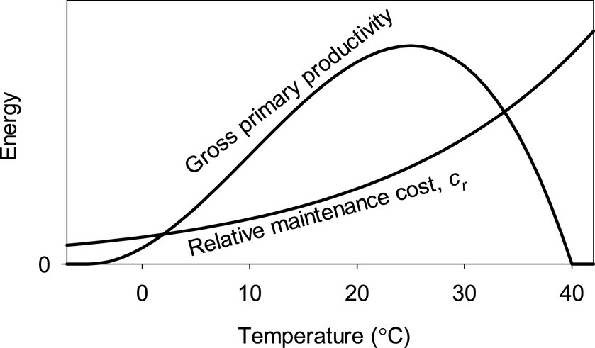
Figure 1. Temperature dependency of pg, i.e., the gross primary productivity of a closed canopy forest or more generally gross primary productivity, and cr, i.e., relative maintenance cost, assuming no diurnal or seasonal temperature variation. The scale on the y-axis is not the same for both curves except at the bottom with zero-value. The models were parameterized in an earlier study (Larjavaara and Muller-Landau, 2012, 2013).
2.3 Biomass accumulation after canopy closure
The energy-based approach has been applied to undisturbed or old-growth forests, as explained above, but its main benefit lies in the possibility of also applying it to successional forests, which has not been done before. The term pn in Eq. 1 changes along a forest succession, but pg in Eq. 2 can be assumed constant after canopy closure (Kira and Shidei, 1967). By definition, a forest is successional when b is smaller than bm and surplus energy is therefore available for b accumulation or Δb:
where h is an efficiency parameter for converting surplus carbon or energy into Δb and discussed more later. To solve Δb, Eq. 3 converts to:
Note that Δb is smaller than gross growth of trees in many successional forests because tree mortality reduces Δb. Eq. 3 is a satisfactory approximation for modeling Δb in various climates. However, several complicating factors can naturally be included in the modeling. For example, pg may change during succession due to more challenging water transport to the crowns of taller trees or due to the scarcity of critical elements in the soil later during succession due to their accumulation in trees (Ryan et al., 2006).
2.4 Biomass accumulation before canopy closure
Modeling pp, i.e., gross primary productivity before canopy closure, is more challenging because a great range of successional patterns is possible. In general, leaf area increases from the start of succession until canopy closure, but, e.g., the temporal changes in the number of tree individuals per unit land area vary and influence how leaf area and thus pp increase. Ideally, pp should not be modeled simply based on the development of individual trees but the changing density of trees should be taken into account. A plantation can be established by planting seedlings that then grow, with the number of trees remaining the same. However, normally more trees germinate during succession and many die. The number of trees can increase or decrease along succession and influence pp. Furthermore, even if leaf area was known, self-shading increases with increasing leaf area lowering pp per leaf area. Because of this complex variation, we decided to simply assume that primary productivity depends on b in the way same as maintenance cost of biomass. Mathematically, the modelling pp was based on the same exponent f, that is used to model consumption to maintain b in Eq. 3:
where bc is above-ground biomass at canopy closure. Surplus energy is used for Δb similarly as after canopy closure, and substituting pg of Eq. 3 with how pp is expressed with pg in Eq. 5 leads to:
and when solved for Δb:
2.5 Biomass accumulation based on relative productivity and relative maintenance cost
The three sections above from 2.2 to 2.4 describe the fundamental logic in the models. In this section we introduce two concepts that will assist in applying the parameterized models to understanding forests dynamics around the world. We defined pr, relative productivity as:
Combining Eqs. 7 and 8 leads to:
Because the values of parameters h and f are invariable globally, for a given b before canopy closure, Δb is proportional to the difference between pr and cr, both of which depend on temperature and pr also depends to some extent on sun elevation.
The energetics of forests with higher biomass differ from those before canopy closure. For old-growth forests, Eq. 2 can be rewritten when combined with Eq. 8:
As f and bc are invariable globally, a larger ratio of pr to cr implies a larger bm. In other words, while the difference between pr and b is proportional with the Δb of small b forests, the quotient between them describes bm in a non-linear manner. Both the difference and quotient can be computed for all humid locations of the world indicating their potential for fast regrowth or for high maximal above-ground biomass. Figure 2 shows the dependence of the difference and quotient assuming an invariable temperature.
Figure 2. Temperature dependency of the difference and quotient of relative productivity, pr, and relative maintenance cost, cr, assuming no diurnal or seasonal temperature variation, a 12 h day, and sun elevation of 90° at solar noon. Temperatures above 30°C are not shown as humid area with those temperatures are not found on Earth (Wright et al., 2009), and the aim of this figure is to show how the quotient peaks at lower temperature than the difference. Temperatures in which pr is positive but smaller than cr (−5°C–2°C with the assumptions in this figure) canopy cannot close. See Section 2.5 for more on pr and cr.
2.6 Data for parameterization
To compile a data set to parametrize parameters bc and h, we searched for peer-reviewed publications from Web of Science and Google Scholar until April 2021. We followed the PRISMA guidelines on searches and inclusion (Liang et al., 2020). We used the following keywords and terms: (“above-ground biomass”* OR “AGB”* OR “carbon storage”*) AND (“natural forest”* OR “secondary forest*” OR “planted forest*” OR “plantation*”) AND (“stand development*” OR “age*”). We then screened all these publications based on their title, abstract, and keywords. We used the following criteria to include studies: (1) the study focused on forest plantations or successional natural forests including both early and more mature stages; (2) the study provided biomass and stand age; (3) sites that had not undergone major natural disturbance, with site mortality >10% of trees or thinning. In the end, we had 630 records from 66 time series and sites and from 44 publications. We extracted the data from tables or digitized graphs using WebSiteDigitizer-4 software. This data and references are available as Supplementary material 1.
In addition, we searched for published databases on b. We found the Global Forest Carbon Database (ForC) (Anderson-Teixeira et al., 2016, 2018) and the Forest Biomass Database of Eurasia (Schepaschenko et al., 2017). ForC contains measurement records of forest carbon stocks, compiled from original publications and earlier data compilations and databases. Measurement records included location, dominant plant functional type, stand age, and measurement methods. Data of b in ForC are measured directly in the field or estimated by allometric relations. The database does not include more indirectly modeled estimates or estimates based on remote sensing. ForC does not include sites that have undergone significant management or other significant disturbances since the most recent stand initiation event. We selected 843 records from 96 sites from this data set. The Forest Biomass Database of Eurasia was compiled from a combination of field surveys undertaken by the authors and from scientific publications that recorded biomass, location, tree species composition, forest functional type, stand age, number of trees per hectare, and number of trees selected for destructive sampling. Data presented in the Forest Biomass Database of Eurasia were collected using in-situ destructive sampling measurements to quantify tree biomasses. We selected 1,775 records that met our criteria from this data set, from 161 sites.
Our database, compiled from the above-mentioned sources, contains geographic information [longitude, latitude, and elevation obtained from either a global data set (Danielson and Gesch, 2011) or the original sources], forest type, forest age, and b. When the measurements were originally expressed in carbon, we converted the carbon masses to biomasses using the IPCC default assumption that 47% of biomass is carbon (Allen et al., 2019). Our database included data from 209 sites of secondary natural forests and 112 sites of managed forests, with 3,177 records in total (Figure 3). Plot size varied but was typically one hectare.
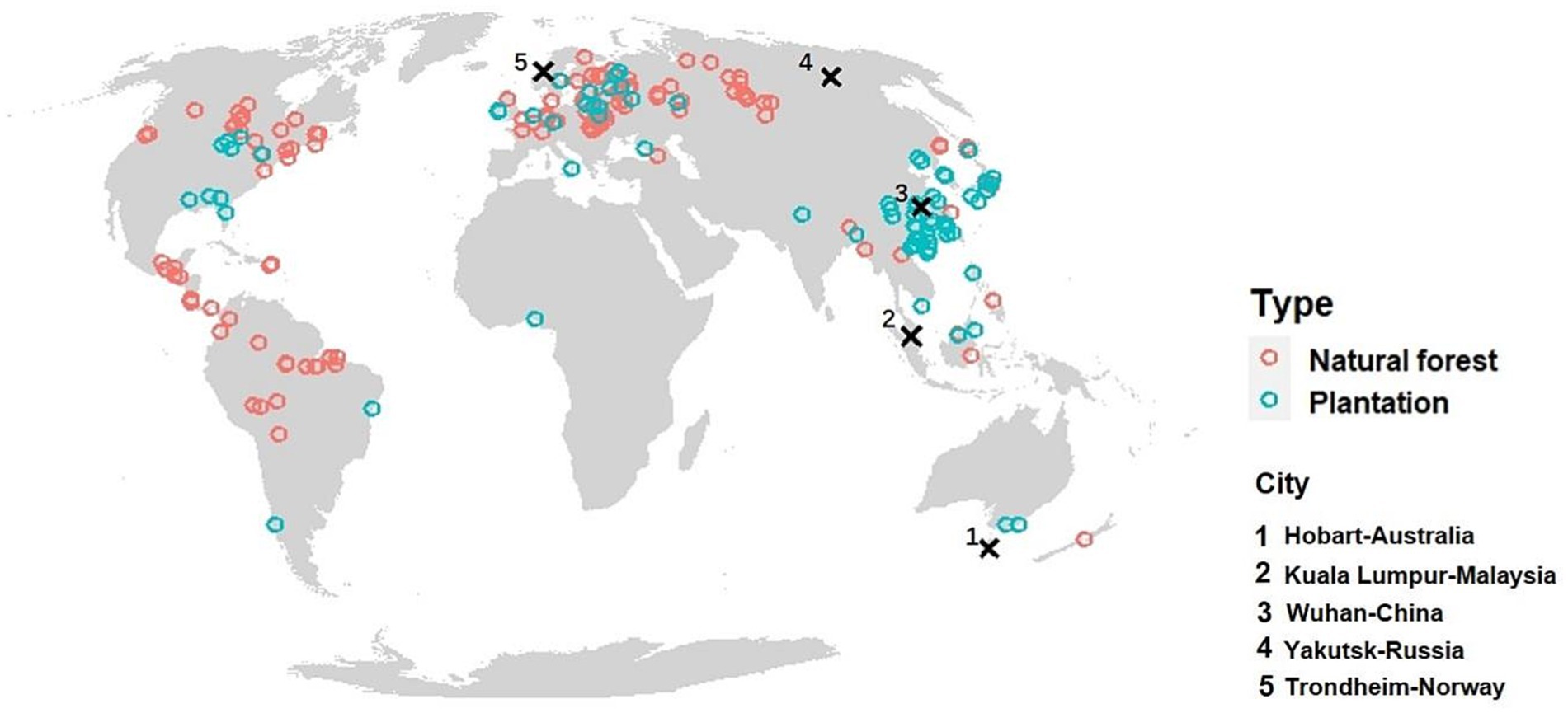
Figure 3. Location of 165 natural forests sites and 83 plantation sites from which data on above-ground biomass, b, was used to parameterize the model. The climate of the five cities shown with large crosses was used to demonstrate how climate influences b in Figures 6, 8.
We extracted the monthly near-surface air temperatures and precipitation for 1970–2000 using the WorldClim database (Fick and Hijmans, 2017). This period corresponded approximately the time when most of the successional forests in the dataset had developed, but is significantly warmer for the early development of the oldest forests and colder for the latest years of most recently measured plots. Even though our main focus was on the patterns of the recent decades, we wanted in addition to understand how rising temperatures impacts these patterns. For this, we extracted 2,081–2,100 monthly average temperatures at a 10 min spatial resolution from WorldClim under the Shared Socio-economic Pathways (SSPs) 245 emission scenario (Fricko et al., 2017), which was simulated from CMIP6 projections.
In the earlier studies on bm on which our study is partly grounded, parameterization was based on humid lowland forests to lower the unexplained variation caused by the impact of water scarcity and direct impact of air pressure (Larjavaara and Muller-Landau, 2012, 2013). In the same way, here we included only lowland areas at elevations below 1,000 m and in which potential evapotranspiration based on a simple method based on mean monthly temperatures and daylight hours (Thornthwaite, 1948) was lower than precipitation. Naturally, water availability could had been included in the modelling by parameterizing, e.g., the impact of the ratio of potential evaporation and precipitation its impact on p. However, this could had been challenging as trees in dry climates can grow well if they obtain water from deep soil layers (Zhang et al., 2017), and secondly, dry climates are susceptible to fires that may hold back forest succession (Sankaran et al., 2005).
2.7 Parameterization technique
We assumed that all parameters related to old-growth forests were the same as in earlier publications (Larjavaara and Muller-Landau, 2012; Larjavaara et al., 2021b). Most of these parameters influence pg and cr. Their impact is reflected in Figure 1 but the original publications (Larjavaara and Muller-Landau, 2012, 2013) should be referred for the detailed picture. In addition to the parameters that determine pg and cr and are not shown above, the parameter f from Eq. 2 influenced parameterization of cr, and therefore we used the same value 0.4 (Larjavaara and Muller-Landau, 2013).
The remaining two parameters, were bc, i.e., biomass at canopy closure and h, i.e., the efficiency of converting surplus energy into biomass accumulation, Δb. In our parameterization, pg was based on carbon assimilated in Mg ha−1 year−1, while Δb was measured in the same unit but include all elements in b rather than just carbon. Therefore, e.g., an efficiency h of 1 would indicate that a Mg of assimilated carbon leads to a Mg of accumulated b. Increasing growth respiration decreases its value.
The sites in our database had time series of b, labeled . The length of a time series was . The recording time steps were . We labeled the biomass bj,i where . For each time series , , and values were and . Note that the observations of and contained uncertainties, and we assumed that
where and denote the observed values and and denote the unobserved true values.
In the dynamical model, we assumed the initial value of biomass to be an unknown parameter . For each , Eqs. 7 and 4 gave us the predicted values of bj,i. We assumed the observed values of biomass to follow:
Based on Eqs. 4, 7, 11–13, we constructed a Bayesian statistical model on biomass growth. As a nonlinear dynamic model, it is more suitable for Bayesian methods. The input data were and bj,i,ob for and . We chose the prior distributions of parameters as , , , , where denotes the exponential distribution with mean and denotes the uniform distribution in the interval . We fitted the posterior distribution of parameters in the model using Stan (Carpenter et al., 2017) with R using package rstan, separately for the whole dataset, for plantations only and for natural forests only.
3 Results
The 3,177 records of b, i.e., biomass at time t since the start of succession, had a range of 0–539.1 Mg ha−1 and an average of 122.8 Mg ha−1. The average time since the start of succession was 41.5 years and the range was from 1 to 400 years. The largest number (1,007) of records were from boreal and continental climates, followed by boreal and maritime climates (852), and tropical (777), temperate and continental (381), and temperate and maritime (160) climates, based on the climate classification described later in the caption of Figure 4.
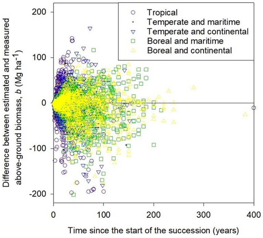
Figure 4. Error in modeled above-ground biomass, b. Tropical climates had mean annual temperatures exceeding 20°C, temperate climates had mean annual temperature under 20°C but at least 10°C, and boreal climates were colder than temperate climates. Temperate and boreal climates were further divided into maritime and continental. In this figure, “maritime” was used to climates in which the difference between warmest and coldest month was less than the difference of thirty and the mean annual temperature as opposite to “continental.”
Biomass accumulation, Δb, was similar in both natural forests exhibiting secondary succession and in managed plantations (Table 2). The best fit value for the parameter bc, biomass at canopy closure, was about 40 Mg ha−1 for both forest types. Parameter h on efficiency of using surplus carbon to Δb, was somewhat larger for plantations than for natural forests but the credible intervals overlapped. The overall value of 0.31 indicates that the photosynthesis of 1 kg of surplus carbon not needed for maintaining b leads to 0.31 kg of Δb, i.e., biomass accumulation, approximately half of which is carbon (Martin et al., 2018).
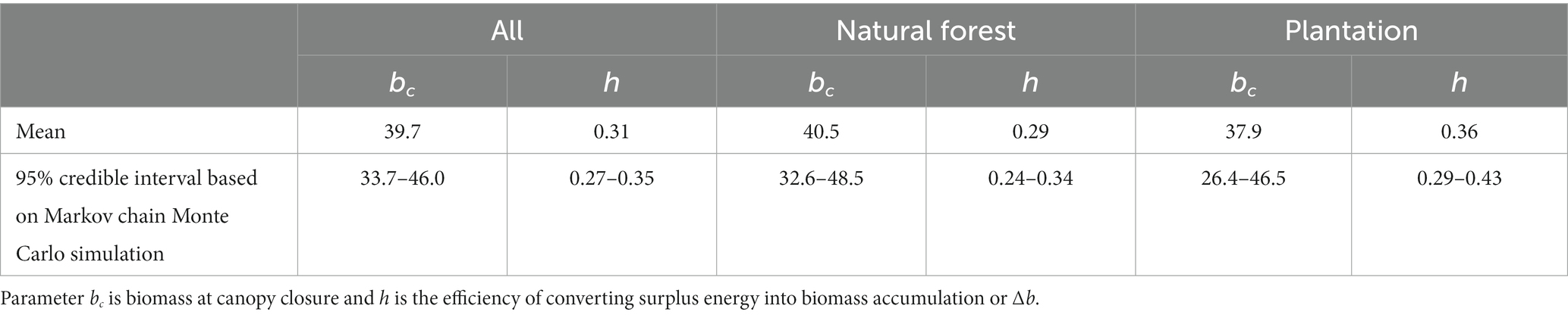
Table 2. Fitted parameter values and associated uncertainty.
Figure 5 illustrates how the different temperature dependencies of relative productivity, pr, and relative maintenance cost, cr, and increasing relative significance of maintenance on energy budgets lead to decreasing optimal temperature for highest Δb with increasing b. The theoretically optimal temperature for Δb before canopy closure assuming a 12 h day and sun elevation of 90° at solar noon was 22.3°C and decreased to 16.4°C just below the globally highest maximal biomass, bm, value of 867 Mg ha−1 reached after a long period without disturbances. In other temperatures, Δb ceases already at lower values of b. However, bm may be higher with temperature variation where temperatures are lower during negative sun elevations because of colder nights but also because of longer nights in winter, as only maintenance cost matters at nighttime.
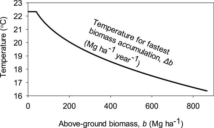
Figure 5. Dependence of a constant air temperature that leads to fastest biomass accumulation, Δb, based on the parameterized model. Here we assumed no diurnal or seasonal temperature variation, a 12 h day, and sun elevation of 90° at solar noon.
We selected five eastern hemisphere cities with strikingly contrasting climates to compare patterns of Δb (Figure 6). The tropical climate represented by Kuala Lumpur had the fastest initial Δb, but the much cooler temperate and ultra-maritime climate of Hobart led to a more prolonged fast Δb later in the succession and a significantly larger bm. The temperate and ultra-continental climate of Wuhan led to a similar pattern as the tropical climate of Kuala Lumpur but with lower values. Despite the gentle start with Δb in the boreal and ultra-maritime climate of Trondheim, significant Δb continued for a long time and resulted in a bm that is not far from the level in much warmer Wuhan. The boreal and ultra-continental climate of Yakutsk led to a slow Δb and low bm.
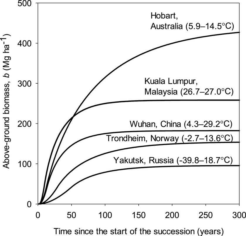
Figure 6. Modeled above-ground biomass, b, accumulation in the climates of five selected cities for 1970–2000 representing extremes of continentality in the boreal and temperate biomes and tropical climate. The temperatures are air temperatures for January and July with the colder value first.
The distribution of errors, i.e., deviance of modelled values from measured ones, was approximately symmetrical for data from all five climatic zones but the estimated values were slightly lower than measured (Figure 4). The mean errors for the five climatic groups were: −2.5 Mg ha−1 for tropical, −1.4 Mg ha−1 for temperate and maritime, −5.6 Mg ha−1 for temperate and continental, −8.8 Mg ha−1 for boreal and maritime and 8.0 Mg ha−1 for boreal and continental. The extreme outliers are at the bottom of the graph, indicating that measured values of b were much higher than modeled values. Similar overestimations are impossible because negative measured values of b are not possible.
Time to canopy closure was shortest in the tropics and subtropics and prolonged at higher latitudes (Figure 7). The difference and quotient of relative productivity, pr, and relative maintenance cost, cr, similarly decreased in general from the equator towards the poles, but pr/cr is also high in temperate regions with a maritime climate (Figure 7). Similar maps for the arid regions of the world are available as Supplementary material 2, but these should be examined very cautiously understanding that the underlying models were parameterized with data from humid regions only.
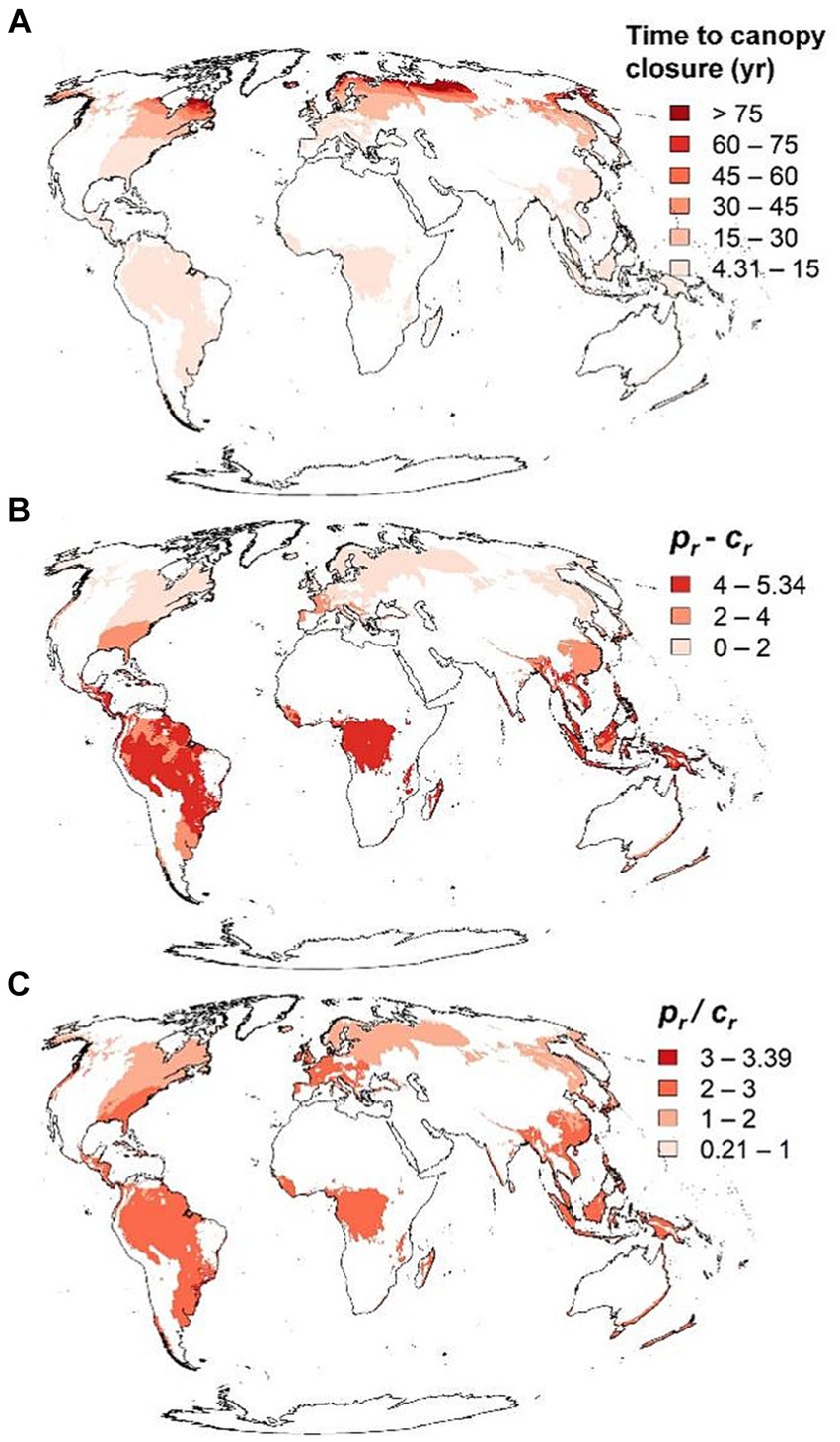
Figure 7. Time to canopy closure, and difference and quotient relative productivity, pr, and relative maintenance cost, cr in humid regions of the word based on temperatures from 1970–2000. See Section 2.5 for more on pr and cr. Maps showing these same variables for arid regions are available in as Supplementary material 2 but note that the models were parameterized based only on humid forests.
The increasing temperatures significantly reduced both pr − cr and pr/cr in the climates of Kuala Lumpur and Wuhan (Figure 8), implying that both the future initial speed of b and bm decreased. The opposite was true for the maritime climates of Hobart and Trondheim. The predicted changes due to increasing temperatures were small for Yakutsk.
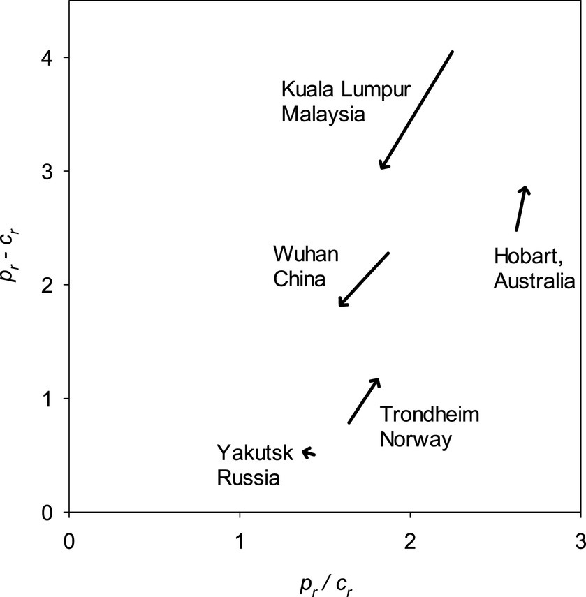
Figure 8. Impact of change in temperatures from 1970–2000 to 2081–2,100 on the difference and quotient of relative productivity, pr, and relative maintenance cost, cr, for temperature regimes of five cities representing differing climates. See Section 2.5 for more on pr and cr. Note that it was assumed that the climates of these locations remain humid in the future.
4 Discussion
We modeled the biomass accumulation speed, Δb, from the same temperature-based physiological perspective that has been used to explain the global variation in biomass of old-growth forests, bm (Larjavaara and Muller-Landau, 2012, 2013). After compiling a large data set of successional forests, we parameterized the two parameters that we assumed to be globally invariable. Based on our results, the temperature for fastest Δb decreases with increasing b. Therefore, warmer climates have the rapid Δb of young forests, while colder climates have larger bm. The mismatch between pn or net primary productivity and bm has been discussed (Keeling and Phillips, 2007), but despite the potentially significant implications, we are not aware of other mechanistic approaches focusing on temperature-driven differences in how ecosystems cycle and store carbon and highlighting these global trends. Instead, much focus has been placed on more local scales. For example, slow growth of large tropical trees during warm years (Clark et al., 2003), extreme productivity of young tree plantations in warmest humid climates (Schroeder, 1992) and occurrence of largest trees on Earth in maritime temperature climates (Larjavaara, 2014), has gained interest. These observations can be explained convincingly based on our modelling approach.
Mean annual temperature variation has played a central role in explaining global patterns in macroecological research (e.g., Wang et al., 2009). Seasonal temperature variation has received less attention, even though it is clear from non-linear temperature sensitivities of photosynthesis and maintenance costs that annual averages may be misleading. Common sense dictates that if an optimal temperature exists for the rapid Δb of young forests or for bm, any seasonal temperature deviation away from this optimum will have negative impacts. This is approximately true based on our modeling, even though the shorter days and lower sun elevations of winters outside the tropics will lower the optimal temperature relative to summers. Interestingly, with suboptimal mean annual temperatures, the seasonal temperature variation can either increase or decrease both the pr − cr, indicating the speed of Δb in young forests and pr/cr that reveals how much b the climate can sustain energetically. In mean annual temperatures that are warmer than the optimal, seasonal temperature variations have a negative impact on both pr − cr and pr/cr, as cr increases exponentially with temperature. However, in cold climates both pr − cr and pr/cr increase with increasing seasonal temperature variation because with constant temperatures the whole year is too cold for pg. Extreme seasonal temperature variation, e.g., the climate of Yakutsk (Figure 6), enables a growing season despite a mean annual temperature well below freezing.
Our methological approach lies closer to the process-based or mechanic models in the continuum from those to purely empirical models in which parameters are obtained statistically without understanding of the underlying processes. Therefore, all the three parameters, f, bc, and h can be discussed from an ecological perspective. We used for parameter f the value 0.4 obtained from an earlier study (Larjavaara and Muller-Landau, 2013), as reparameterizing it for the successional forests would have required reparameterization of cr at the same time. Faster accumulation of non-metabolizing heartwood with increasing b, would lower the value of f. The best fit value of 40 Mg ha−1 for parameter bc (Table 2), was within the expected range and the time required to reach this b varies considerable depending on the climate (Figure 6). The value of 0.31 for parameter h (Table 2) was surprisingly low as indicates that only some 15% of the photosynthesized carbon not needed for maintaining the given b, ends up increasing b. However, this number should not be compared directly to parameter values in more conventional approaches when all growth, even to maintain a given b, is included. Expectedly, plantations had higher h compared with natural forests (Table 2), as species selection, planting density and other management decisions have been taken to aim rapid growth.
Expectedly, our data set on b in successional forests had plenty of unexplained variation (Figure 4). Despite of this, we argue that our simple process-based modelling is especially valuable to stimulate new thinking as it is faster to understand than complex and normally more realistic approaches. Nevertheless, many possibilities exist to increase complexity and possibly the fit. As we applied the temperature-driven energetic modeling approach, we excluded factors like previous land use legacies and variations in small-scale disturbances or other aspects such as the liana load in the tropics (Finlayson et al., 2022) or minor management actions in plantations during succession that may influence Δb. However, these factors are likely to not cause significant biases but more symmetric variation, as seen in Figure 4. More dangerous biases may result from the basic assumption of the modeling approach. For example, the assumption of constant pg after canopy closure may be false if older and larger trees face challenges in transporting water upwards or carbohydrates downwards or if larger b locks more nutrients in the woody tissue and makes these unavailable for leaf and below-ground processes. Unfortunately, the scatter in our data set makes the examination of these successional changes impossible. One potential future research direction would be to reparametrize the models on temperature and sun elevation dependence based on data from successional forests with pg measured. Such data sets are available (West, 2020), and this approach could, e.g., lead to improved estimation of parameter f in successional forests. Other potential directions in which complexity could be added, would be to parameterize the model separately for each taxonomic (e.g., gymnosperms and angiosperms) or functional tree type (e.g., evergreen vs. deciduous), and separately into various climatic regions. However, these factors are likely to have only a small impact on the parameters. Parameter bc is fundamentally dependent on wind regimes and gravity (Larjavaara et al., 2021a). Therefore, as our model is particularly well suited for global analyses.
Our modeling approach offers a relatively simple and novel perspective to understanding global terrestrial carbon cycling and can be applied to understanding the impact of climate change on forests and to mitigating climate change with forests. Our modeling reveals both the ability of young forests to accumulate b rapidly and bm to decline dangerously in the future in tropical, and temperate and continental climates with hot summers (Figure 8). Our temperature-based approach to understanding variation in Δb depending on accumulated b may be used to optimize land use globally for mitigating climate change without sacrificing wood production. For example, when focusing solely on wood production and carbon storage, the rapid early accumulation of b relative to pg in the tropics and temperate and continental climates make these areas more suitable for wood production than for storing carbon relative to more maritime temperate and boreal climates.
Data availability statement
The original contributions presented in the study are included in the article/Supplementary material, further inquiries can be directed to the corresponding authors.
Author contributions
MLa developed the research idea and wrote most of the first version of the manuscript. XC collected the data. MLu and XC parameterized the models. All authors contributed to the article and approved the submitted version.
Funding
We thank National Natural Science Foundation of China, no: 32171539, National key Research and Development Program of China, no: 2023YFE0105100-1 and Peking University.
Acknowledgments
We thank Annikki Mäkelä for discussions, Stella Thompson for linguistic revision.
Conflict of interest
The authors declare that the research was conducted in the absence of any commercial or financial relationships that could be construed as a potential conflict of interest.
Publisher’s note
All claims expressed in this article are solely those of the authors and do not necessarily represent those of their affiliated organizations, or those of the publisher, the editors and the reviewers. Any product that may be evaluated in this article, or claim that may be made by its manufacturer, is not guaranteed or endorsed by the publisher.
Supplementary material
The Supplementary material for this article can be found online at: https://www.frontiersin.org/articles/10.3389/ffgc.2024.1142209/full#supplementary-material
References
Acharya, R. P., Maraseni, T., and Cockfield, G. (2019). Global trend of forest ecosystem services valuation—an analysis of publications. Ecosyst. Serv. 39:100979. doi: 10.1016/j.ecoser.2019.100979
Adebayo, A. B., Han, H.-S., and Johnson, L. (2007). Productivity and cost of cut-to-length and whole-tree harvesting in a mixed-conifer stand. For. Prod. J. 57:59.
Allen, M., Antwi-Agyei, P., Aragon-Durand, F., Babiker, M., Bertoldi, P., Bind, M., et al., (2019). Technical summary: global warming of 1.5 C. An Ipcc special report on the impacts of global warming of 1.5 C above pre-industrial levels and related global greenhouse gas emission pathways, in the context of strengthening the global response to the threat of climate change, sustainable development, And Efforts To Eradicate Poverty
Anderson, K. J., Allen, A. P., Gillooly, J. F., and Brown, J. H. (2006). Temperature-dependence of biomass accumulation rates during secondary succession. Ecol. Lett. 9, 673–682. doi: 10.1111/j.1461-0248.2006.00914.x
Anderson-Teixeira, K. J., Herrmann, V., Morgan, R. B., Bond-Lamberty, B., Cook-Patton, S. C., Ferson, A. E., et al. (2021). Carbon cycling in mature and regrowth forests globally. Environ. Res. Lett. 16:abed01. doi: 10.1088/1748-9326/abed01
Anderson-Teixeira, K. J., Wang, M. M., Mcgarvey, J. C., Herrmann, V., Tepley, A. J., Bond-Lamberty, B., et al. (2018). ForC: a global database of forest carbon stocks and fluxes. ECY 99:1507. doi: 10.1002/ecy.2229
Anderson-Teixeira, K. J., Wang, M. M. H., Mcgarvey, J. C., and Lebauer, D. S. (2016). Carbon dynamics of mature and regrowth tropical forests derived from a pantropical database (Tropforc-Db). Glob. Chang. Biol. 22, 1690–1709. doi: 10.1111/gcb.13226
Aubinet, M., Vesala, T., and Papale, D. (2012). Eddy covariance: a practical guide to measurement and data analysis Springer Science & Business Media.
Carpenter, B., Gelman, A., Hoffman, M. D., Lee, D., Goodrich, B., Betancourt, M., et al. (2017). Stan: a probabilistic programming language. J. Stat. Softw. 76, 1–29. doi: 10.18637/jss.v076.i01
Carvalhais, N., Forkel, M., Khomik, M., Bellarby, J., Jung, M., Migliavacca, M., et al. (2014). Global covariation of carbon turnover times with climate in terrestrial ecosystems. Nature 514:213. doi: 10.1038/nature13731
Clark, D. A., Piper, S. C., Keeling, C. D., and Clark, D. B. (2003). Tropical rain forest tree growth and atmospheric carbon dynamics linked to interannual temperature variation during 1984–2000. Proc. Natl. Acad. Sci. USA 100, 5852–5857. doi: 10.1073/pnas.0935903100
Cook-Patton, S. C., Leavitt, S. M., Gibbs, D., Harris, N. L., Lister, K., Anderson-Teixeira, K. J., et al. (2020). Mapping carbon accumulation potential from global natural Forest regrowth. Nature 585, 545–550. doi: 10.1038/s41586-020-2686-x
Danielson, J. J., and Gesch, D. B., (2011). Global multi-resolution terrain elevation data 2010 (Gmted2010), US Department Of The Interior, US Geological Survey Washington, DC, USA
Ellison, D., Morris, C. E., Locatelli, B., Sheil, D., Cohen, J., Murdiyarso, D., et al. (2017). Trees, forests and water: cool insights for a hot world. Glob. Environ. Chang. 43, 51–61. doi: 10.1016/j.gloenvcha.2017.01.002
Fick, S. E., and Hijmans, R. J. (2017). Worldclim 2: new 1-km spatial resolution climate surfaces for global land areas. Int. J. Climatol. 37, 4302–4315. doi: 10.1002/joc.5086
Finlayson, C., Roopsind, A., Griscom, B. W., Edwards, D. P., and Freckleton, R. P., (2022). Removing climbers more than doubles tree growth and biomass in degraded tropical forests. Ecol. Evol., 12, e8758, doi: 10.1002/ece3.8758
Fricko, O., Havlik, P., Rogelj, J., Klimont, Z., Gusti, M., Johnson, N., et al. (2017). The marker quantification of the shared socioeconomic pathway 2: a middle-of-the-road scenario for the 21st century. Global Environmental Change-Human Policy Dimensions 42, 251–267. doi: 10.1016/j.gloenvcha.2016.06.004
Hurmekoski, E., Smyth, C. E., Stern, T., Verkerk, P. J., and Asada, R. (2021). Substitution impacts of wood use at the market level: a systematic review. Environ. Res. Lett. 16:123004. doi: 10.1088/1748-9326/ac386f
Keeling, H. C., and Phillips, O. L. (2007). The global relationship between forest productivity and biomass. Glob. Ecol. Biogeogr. 16, 618–631. doi: 10.1111/j.1466-8238.2007.00314.x
Kira, T., and Shidei, T. (1967). Primary production and turnover of organic matter in different forest ecosystems of the Western Pacific. Japanese J. Ecol. 17, 70–87. doi: 10.18960/seitai.17.2_70
Kirch, P. (2005). Archaeology and global change: the Holocene record. Annu. Rev. Environ. Resour. 30, 409–440. doi: 10.1146/annurev.energy.29.102403.140700
Kolis, K., Hiironen, J., Ärölä, E., and Vitikainen, A. (2014). Effects of Sale-specific factors on stumpage prices in Finland. Silva Fennica 48:e1054. doi: 10.14214/sf.1054
Kuusinen, N., Kolari, P., Levula, J., Porcar-Castell, A., Stenberg, P., and Berninger, F. (2012). Seasonal variation in boreal pine forest albedo and effects of canopy snow on forest reflectance. Agric. For. Meteorol. 164, 53–60. doi: 10.1016/j.agrformet.2012.05.009
Larjavaara, M. (2014). The World's tallest trees grow in thermally similar climates. New Phytol. 202, 344–349. doi: 10.1111/nph.12656
Larjavaara, M. (2021). What would a tree say about its size? Front. Ecol. Evol. 8:564302. doi: 10.3389/fevo.2020.564302
Larjavaara, M., Auvinen, M., Kantola, A., and Mäkelä, A. (2021a). Wind and gravity in shaping Picea trunks. Trees Structure & Functioning 35, 1587–1599. doi: 10.1007/s00468-021-02138-3
Larjavaara, M., Davenport, T. R. B., Gangga, A., Holm, S., Kanninen, M., and Tien, N. D. (2019). Payments for adding ecosystem carbon are mostly beneficial to biodiversity. Environ. Res. Lett. 14:e1554. doi: 10.1088/1748-9326/ab1554
Larjavaara, M., Lu, X., Chen, X., and Vastaranta, M. (2021b). Impact of rising temperatures on the biomass of humid old-growth forests of the world. Carbon Balance Manag. 16:31. doi: 10.1186/s13021-021-00194-3
Larjavaara, M., and Muller-Landau, H. C. (2012). Temperature explains global variation in biomass among humid old-growth forests. Glob. Ecol. Biogeogr. 21, 998–1006. doi: 10.1111/j.1466-8238.2011.00740.x
Larjavaara, M., and Muller-Landau, H. C. (2013). Corrigendum on: temperature explains global variation in biomass among humid old-growth forests (Vol 21, Pg 998, 2012). Glob. Ecol. Biogeogr. 22:772. doi: 10.1111/geb.12037
Lewis, S. L., Wheeler, C. E., Mitchard, E. T., and Koch, A. (2019). Restoring natural forests is the best way to remove atmospheric carbon. Nature 568, 25–28. doi: 10.1038/d41586-019-01026-8
Liang, X. Y., Zhang, T., Lu, X. K., Ellsworth, D. S., Bassirirad, H., You, C. M., et al. (2020). Global response patterns of plant photosynthesis to nitrogen addition: a meta-analysis. Glob. Chang. Biol. 26, 3585–3600. doi: 10.1111/gcb.15071
Malhi, Y. (2010). The carbon balance of tropical Forest regions, 1990–2005. Curr. Opin. Environ. Sustain. 2, 237–244. doi: 10.1016/j.cosust.2010.08.002
Malhi, Y., Doughty, C., and Galbraith, D. (2011). The allocation of ecosystem net primary productivity in tropical forests. Philos Trans R Soc Lond B 366, 3225–3245. doi: 10.1098/rstb.2011.0062
Martin, A. R., Doraisami, M., and Thomas, S. C. (2018). Global patterns in wood carbon concentration across the World's trees and forests. Nat. Geosci. 11, 915–920. doi: 10.1038/s41561-018-0246-x
Martin, A. R., and Thomas, S. C. (2011). A reassessment of carbon content in tropical trees. PLoS One 6:e23533. doi: 10.1371/journal.pone.0023533
Miina, J., Hotanen, J.-P., and Salo, K., (2009). Modelling the abundance and temporal variation in the production of bilberry (Vaccinium Myrtillus L.) In Finnish Mineral Soil Forests
Muller-Landau, H. C., Cushman, K. C., Arroyo, E. E., Cano, I. M., Anderson-Teixeira, K. J., and Backiel, B. (2021). Patterns and mechanisms of spatial variation in tropical Forest productivity, Woody residence time, and biomass. New Phytol. 229, 3065–3087. doi: 10.1111/nph.17084
Pangala, S. R., Enrich-Prast, A., Basso, L. S., Peixoto, R. B., Bastviken, D., Hornibrook, E. R., et al. (2017). Large emissions from floodplain trees close the Amazon methane budget. Nature 552, 230–234. doi: 10.1038/nature24639
Peltzer, D. A., Wardle, D. A., Allison, V. J., Baisden, W. T., Bardgett, R. D., Chadwick, O. A., et al. (2010). Understanding ecosystem retrogression. Ecol. Monogr. 80, 509–529. doi: 10.1890/09-1552.1
Penman, J., Gytarsky, M., Hiraishi, T., Krug, T., Kruger, D., Pipatti, R., et al., (2003). Good practice guidance for land use, land-use change and forestry. good practice guidance for land use, land-use change and forestry
Poorter, L., Bongers, F., Aide, T. M., Almeyda Zambrano, A. M., Balvanera, P., Becknell, J. M., et al. (2016). Biomass resilience of neotropical secondary forests. Nature 530, 211–214. doi: 10.1038/nature16512
Pukkala, T. (2016). Which type of forest management provides most ecosystem services? Forest Ecosyst. 3, 1–16.
Ramankutty, N., and Foley, J. A. J. G. (1999). Estimating historical changes in global land cover: croplands from 1700 to 1992. J. Geogr. Inf. Syst. 13, 997–1027. doi: 10.1029/1999GB900046
Ryan, M. G., Binkley, D., Fownes, J. H., Giardina, C. P., and Senock, R. S. (2004). An experimental test of the causes of forest growth decline with stand age. Ecol. Monogr. 74, 393–414. doi: 10.1890/03-4037
Ryan, M. G., Phillips, N., and Bond, B. J. (2006). The hydraulic limitation hypothesis revisited. Plant Cell Environ 29, 367–381. doi: 10.1111/j.1365-3040.2005.01478.x
Ryan, M. G., and Yoder, B. J. (1997). Hydraulic limits to tree height and tree growth. Bioscience 47, 235–242. doi: 10.2307/1313077
Sankaran, M., Hanan, N. P., Scholes, R. J., Ratnam, J., Augustine, D. J., Cade, B. S., et al. (2005). Determinants of Woody cover in African savannas. Nature 438, 846–849. doi: 10.1038/nature04070
Schepaschenko, D., Shvidenko, A., Usoltsev, V., Lakyda, P., Luo, Y. J., Vasylyshyn, R., et al. (2017). A dataset of Forest biomass structure for Eurasia. Sci Data, 4:170070. doi: 10.1038/sdata.2017.70
Schroeder, P. (1992). Carbon storage potential of short rotation tropical tree plantations. For. Ecol. Manag. 50, 31–41. doi: 10.1016/0378-1127(92)90312-W
Sidle, R. C., Ziegler, A. D., Negishi, J. N., Nik, A. R., Siew, R., and Turkelboom, F. (2006). Erosion processes in steep terrain—truths, myths, and uncertainties related to Forest management in Southeast Asia. Forest Ecol. Manag. 224, 199–225. doi: 10.1016/j.foreco.2005.12.019
Thornthwaite, C. (1948). An approach toward a rational classification of climate. Geogr. Rev. 38, 55–94. doi: 10.2307/210739
Turtiainen, M., Miina, J., Salo, K., and Hotanen, J.-P. (2016). Modelling the coverage and annual variation in bilberry yield in Finland. Silva Fennica. 50:1573. doi: 10.14214/sf.1573
Wang, C. (2006). Biomass allometric equations for 10 co-occurring tree species in Chinese temperate forests. For. Ecol. Manag. 222, 9–16. doi: 10.1016/j.foreco.2005.10.074
Wang, Z., Brown, J. H., Tang, Z., and Fang, J. (2009). Temperature dependence, spatial scale, and tree species diversity in eastern Asia and North America. Proc. Natl. Acad. Sci. 106, 13388–13392. doi: 10.1073/pnas.0905030106
West, P. (2020). Do increasing respiratory costs explain the decline with age of Forest growth rate? J. For. Res. 31, 693–712. doi: 10.1007/s11676-019-01020-w
Wright, S. J., Muller-Landau, H. C., and Schipper, J. (2009). The future of tropical species on a warmer planet. Conserv. Biol. 23, 1418–1426. doi: 10.1111/j.1523-1739.2009.01337.x
Keywords: biomass, carbon, climate, energy, forest, growth, model, temperature
Citation: Larjavaara M, Chen X and Luo M (2024) A temperature-based model of biomass accumulation in humid forests of the world. Front. For. Glob. Change. 7:1142209. doi: 10.3389/ffgc.2024.1142209
Edited by:
Ulises Diéguez-Aranda, University of Santiago de Compostela, SpainReviewed by:
Miguel Gonzalez, Guangzhou Institute of Geography, ChinaBrian Russell Sturtevant, Forest Service (USDA), United States
Copyright © 2024 Larjavaara, Chen and Luo. This is an open-access article distributed under the terms of the Creative Commons Attribution License (CC BY). The use, distribution or reproduction in other forums is permitted, provided the original author(s) and the copyright owner(s) are credited and that the original publication in this journal is cited, in accordance with accepted academic practice. No use, distribution or reproduction is permitted which does not comply with these terms.
*Correspondence: Markku Larjavaara, bWFya2t1LmxhcmphdmFhcmFAaGVsc2lua2kuZmk=; Xia Chen, Y2hlbnhpYUB6YWZ1LmVkdS5jbg==
†These authors have contributed equally to this work