Response of spring vegetation phenology to soil freeze–thaw state in the Northern Hemisphere from 2016 to 2022

Introduction: The research on spring vegetation phenology is crucial to the investigation of terrestrial ecosystems and climate change. Changes in the soil freeze–thaw (F/T) lead to variations in soil moisture, directly impacting vegetation activity. The start of the season (SOS) is the initial and important phenophase for vegetation activity, and thus, this highlights the need to understand the response of spring vegetation phenology to soil F/T state.

Methods: This study first comprehensively investigates the consistency of the SOS and three soil F/T state indexes, i.e., the start day of the F/T state (SFT), the end day of the F/T state (EFT), and the length of days of the F/T state (LFT) via satellite data source.

Results: Results reveal that: (1) All 3 F/T state indexes impact SOS values, and the EFT outperforms others. The correlation coefficients between EFT and SOS gain around 3.07%. (2) A temporal overlap between SOS and EFT occurs in May, suggesting that parts of the plants begin active growth before average temperatures reach above 0°. (3) Small differences of SOS and EFT exist between savannas, and croplands, with an average difference of less than 10 days; in contrast, the largest differences occur in broadleaf evergreen forests. The results can fill the knowledge gap on the response of spring vegetation phenology to soil F/T state, and help to investigate the reasons for the nonlinear dynamics of SOS under global warming.

1 Introduction

Spring vegetation phenology is a combination of biological rhythms and environmental conditions, reflecting the prevailing weather conditions and the cumulative effects of meteorological conditions (Schwartz, 1998). It is commonly used in the study of terrestrial ecosystems and global change. Satellite data thus has become a key measure in recent global ecological studies since the 1980s (Myneni et al., 1997; Piao et al., 2015). Accordingly, phenological extraction methods based on satellite products have developed during the past decades (White et al., 2009; Cong et al., 2012; Chen et al., 2022). Among these grided vegetation products, the Normalized Differential vegetation index (NDVI) is the preferred index for biological studies (Zhou et al., 2001) because of the long-term expansion and multiple sources (Myneni et al., 1997; Zhang et al., 2003). The calculation method highlights vegetation information due to the high reflectance of chlorophyll in the near-infrared (NIR) band and strong absorption in the infrared (IR) band (Haboudane et al., 2002).

The start of the season (SOS) has advanced significantly during the past several decades with the continuous warming in most areas of the Northern Hemisphere (Jeong et al., 2011; Li et al., 2022). However, the SOS dynamic does not show a fixed advancing magnitude, and the changing trend is proven by different periods, areas, and vegetation cover (Yu et al., 2010; Piao et al., 2017). Early season temperature is proven to be the main driving factor for SOS in previous studies. At the same time, precipitation interactively regulates SOS variation in arid and semi-arid regions (Shen et al., 2015). To our knowledge, the precipitation effect is mentioned mainly by the part transferring soil moisture underground. Besides precipitation and groundwater, soil moisture comes primarily from the thawing of frozen water in the spring. The soil freeze–thaw (F/T) state responds accordingly to global climate change (Yang et al., 2019). Changes in the soil F/T lead to variations in soil moisture conditions and physical properties, which can directly affect plant activities, such as spring phenology. The start/end time of the soil F/T state also affects the start of the vegetation growing season and thus net primary productivity. Therefore, investigating the response of spring vegetation phenology to soil F/T state is urgently needed for environmental activities. However, to the best of our knowledge, the impact of F/T on SOS has rarely been evaluated due to the lack of datasets.

The soil F/T state is affected by climate change, topography, and vegetation cover, which mainly occurs in high-altitude or high-latitude cryospheres (Jiang et al., 2020). In recent years, the distribution of soil permafrost has changed significantly under the influence of climate warming, and the detection of soil F/T state has gradually become a research hotspot (Kim et al., 2010; Rowlandson et al., 2018; Kim et al., 2019). Methods for determining soil F/T state can be divided into three main categories: in-situ measurement, numerical modeling, and remote sensing methods (Pardo Lara et al., 2020; Wang et al., 2020; Xie et al., 2021). In-situ measurement can accurately obtain the near-surface soil F/T state; however, the spatial continuity of in-situ measurement is limited, and the distribution of observation stations is relatively sparse. It cannot reflect the characteristics of large-scale continuous soil F/T changes. The numerical method can simulate the soil temperature through the land surface process model to judge the soil F/T state. Nevertheless, uncertainty exists in the parameters input for numerical simulations, which may lead to errors for soil F/T state simulations. Microwave remote sensing has a long wavelength, and can penetrate the topsoil surface. Microwave remote sensing is sensitive to the dielectric changes in the soil F/T state when the near-surface soil undergoes the F/T cycle. Active microwave remote sensing, such as Synthetic Aperture Radar (SAR) images, can be an effective tool for soil F/T state detection (Chen et al., 2019). However, active microwave remote sensing is limited by its ability to retrieve high temporal soil F/T state with its long revisit time. Since the successful launch of the passive microwave satellites, e.g., Soil Moisture and Ocean Salinity (SMOS) mission and the NASA Soil Moisture Active Passive (SMAP) mission, an increasing number of studies have been devoted to the development of F/T monitoring algorithms using L-band signals emitted, which is considered to be the optimal band for soil conditions monitoring due to its sensitivity with soil permittivity (Chen et al., 2019; Kim et al., 2019).

This study is motivated to demonstrate the response of spring vegetation phenology to soil F/T state. Here, three indexes, i.e., the start day of the F/T state (SFT), the end day of the F/T state (EFT), and the length days of the F/T state (LFT), are derived from the SMAP F/T product, and their consistencies with the SOS is clarified. In addition, the distribution of SFT, EFT, LFT, and SOS with land cover types is analyzed, and the differences between the SOS and EFT are also investigated. Finally, the factors affecting these relationships are also addressed. The results can deepen the understanding of the influence of soil F/T status on vegetation phenology.

2 Data

2.1 SMAP freeze/thaw data

The SMAP mission, launched by NASA in 2015, operates in the L band. It has a revisit time of 2 ~ 3 days. The 9 km L3 Radiometer Global and Northern Hemisphere Daily F/T data from 2016 to 2022 are used here. The data are selected for the months of March through June of each year. The F/T product is derived from the brightness temperatures. Two observations of the ascent (6:00 PM) and descent (6:00 AM) are provided per day, with “0” indicating thawed conditions, and “1” indicating frozen. Soil F/T state is determined by a baseline method, whereby the time response of the normalized polarization ratio of the brightness temperature is determined. The method is sensitive to changes in the soil permittivity, and apparent changes in soil permittivity as water transitions between freezing and non-freezing conditions (Chew et al., 2017). Data from 2016 to 2022 are collected. The data is then resampled to 10 km using the nearest neighbor interpolation method to match with the NDVI data.

2.2 NDVI data

GIMMS 3 g + NDVI product is used to estimate the SOS. The dataset is produced by Global Inventory Modeling and Mapping Studies (GIMMS) (Tucker et al., 2005). The latest generation GIMMS3g + updates the data to 2022 with biweekly temporal resolution and 1/12° spatial resolution, and we thus get the annual series with 24 components (Cong et al., 2013). We employ data from 2016 to 2022, to be consistent with the period of the F/T data.

2.3 Land cover data

The land cover data employed here is the International Geosphere-Biosphere Programme (IGBP) land classification data. The IGBP is supplied by the MODIS MCD12Q3 product, with a spatial resolution of 1 km. In order to cooperate with the NDVI data, the resolution is then resampled to 10 km.

2.4 Ancillary data

Soil moisture and soil surface temperature for March through June from 2016 through 2022, selected from the ERA5-Land monthly average data, are used for comparison. The resolution of the ERA5-Land monthly data is 0.1°. The soil moisture and surface temperature data are then averaged annually to final values (Supplementary Figure S1).

3 Method

3.1 Extraction method for the start of F/T state (SFT) and end of F/T state (EFT)

A conceptual and simple method is used to identify the state of the soil F/T state (SFT). When a pixel has an F/T state for over four consecutive days, i.e., four consecutive days with am data of 1 and pm data of 0, this day of the year (DOY) is considered the SFT value. Conversely, sorting the data in reverse order by DOY, when a pixel has an F/T state for over four consecutive days, the DOY is considered an EFT value. Besides, the length of the F/T state (LFT) is a necessary index of climate change, which may affect the SOS. Here, the value of the LFT is obtained as the subtraction value of the SFT and EFT.

3.2 Extraction method for the start of the season (SOS)

The polyfit-maximum method is used to estimate SOS in this study. The invalid value is removed from the NDVI time series. The invalid value is defined as the value that is lower than the two neighboring points from March to November. Then, the missing value is mended via simple linear interpolation. A six-degree polynomial model is used here to fit the annual NDVI curves.

y(x) = a₀ + a₁x + a₂x² + a₃x³ + a₄x⁴ + a₅x⁵ + a₆x⁶

where y(x) indicates the NDVI value at the x period; a(_{0, 1, 2, 3, 4, 5, 6}) indicates the fitting coefficients of the least squares in the formula.

The maximum changing ratio is considered to be the active growing season starting dates. The most rapid increase interval of NDVI from March to September is judged to be the start of green-up, and the date of year (DOY) gained based on the annual mean NDVI value of the fastest increasing period. The detailed method can be found in Cong et al. (2012) and Piao et al. (2006).

4 Results

4.1 Spatial distribution of the annual averaged SFT, EFT, LFT, and SOS

Figure 1 shows the spatial distribution of the annual averaged SFT, EFT, LFT, and SOS over the Northern Hemisphere from 2016–2022. The slight changes happen in SFT, with most values concentrated earlier than 80 in Julian day. North of Canada and the Tibetan Plateau regions display relatively high SFT values, both of which have exceeded 100 in Julian day (Figure 1A). These two regions consistently indicate low spring temperature (Supplementary Figure S1A), and the frozen soil thus thaws late. EFT varies more significantly compared to SFT. The larger values in North America and the Tibetan Plateau regions indicate that the F/T state ends later. In addition to these two regions, some parts of southern North America also have larger EFT values, while most of the data in the other regions are earlier than 120 in Julian day (Figure 1B). Regarding the LFT, the LFTs in different areas vary significantly, showing a gradual increase southward. The Tibetan Plateau region and southern North America have relatively larger LFT values, with values longer than 40 in Julian day (Figure 1C). Interestingly, in mid-low latitude areas, we can see that longer LFT corresponds to less soil moisture. This phenomenon is apparent in South Asia and Southwest America. This is probably due to the relatively smaller specific heat capacity of drier soil. For instance, the Tibetan Plateau has very strong radiation in the daytime, and the surface temperature increases quickly in early spring. Meanwhile, the temperature falls below 0 centigrade without sunlight during nighttime. Therefore, the LFT lasts longer for the frequent changes below and above 0°during the whole day.

FIGURE 1

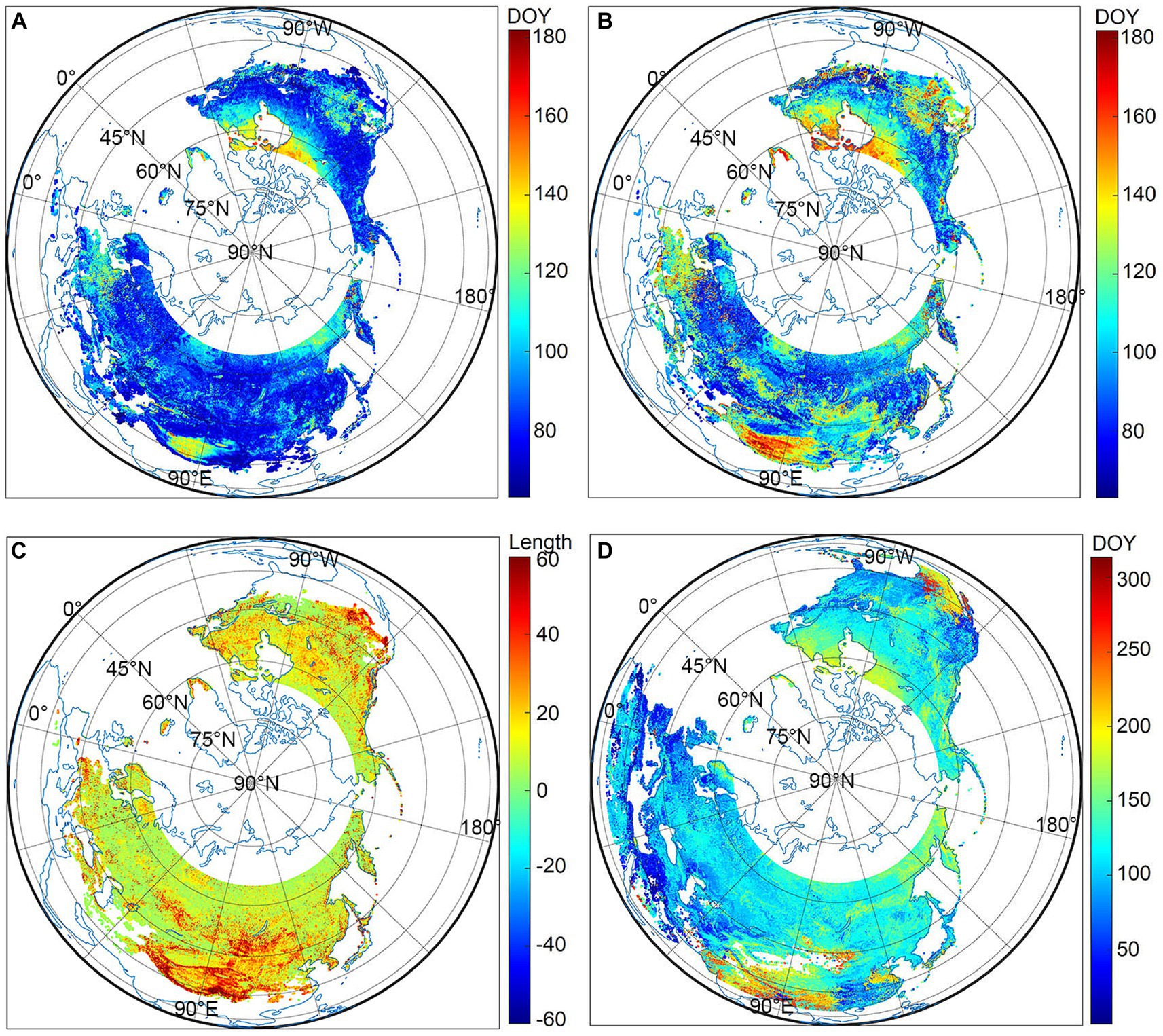
Figure 1. The spatial distribution of averaged SFT, EFT, LEF, and SOS.

Generally, the spatial distribution of SOS is similar to EFT. Variations along latitude also show significant similarities. The averaged SOS pattern in Figure 1D suggests variation along altitude. SOS increases from low latitude to high latitude between March to early June. SOS in North America varies gradually along altitude except for the southern semi-arid region. The grasslands and shrublands with sparse vegetation cover in this region may lead to the relatively late SOS. Furthermore, in Eurasia, vegetation in Europe starts active growth early in the southern area, and the SOS increases northward and eastward. SOS starts late in the Tibetan Plateau in South Asia mainly due to low temperatures resulting from high altitude, while low temperatures result in late green-up of alpine vegetation. In the mid-latitude region of Eurasia, vegetation in Asia starts growing slightly later than in Europe. The high-latitude region shows a similar SOS pattern to the mid-latitude area. Similar to the LFT, the SOS variations also show an inverse tendency with the soil moisture. It can be concluded that soil moisture is a crucial factor in the SOS besides spring temperature.

Global temperatures have risen slowly over the past several years, potentially advancing the spring phenology. The probability density functions (PDF) of SFT, EFT, LFT, and SOS for each year are presented in Figure 2, in order to explore the possible effects of soil F/T on spring phenology. As shown in Figure 2A, the onset of soil F/T state is concentrated in earlier periods, mainly in March and April. The largest proportion occurs in March, with a slight difference among the 7 years.

FIGURE 2

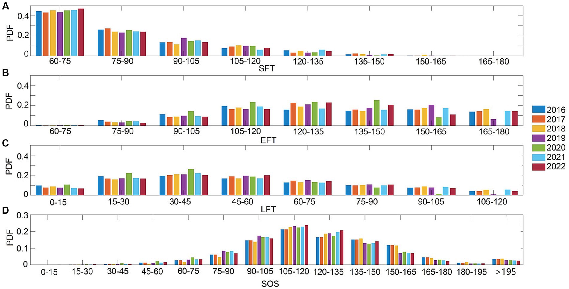
Figure 2. The PDFs of SFT, EFT, LEF, and SOS from 2016 to 2022.

The end of the soil F/T state is mainly concentrated in April to June. The largest fraction occurs in May, while there are some differences among the 7 years, but insignificant (Figure 2B). On an annual basis, the value of LFT continues to fluctuate between 15 and 80 days (Figure 2C). The inter-annual variation in LFT appeared to be smaller than that of EFT (Figure 2B).

The PDF of SOS is distributed normally, mainly concentrating on April and early June. Before mid-May, the PDFs of SOS show an annual increase; conversely, after mid-May, the PDFs decrease slightly. Therefore, SOS indicates an advance tendency from 2016 to 2022 (Figure 2D). Theoretically, SOS should occur after EFT, but the results indicate a temporal overlap between SOS and EFT in May. This suggests that plants begin active growth before average temperatures reach above 0°. The demand for vegetation to start green-up thus varies with the vegetation category and the environmental conditions.

4.2 The distribution of SFT, EFT, LFT, and SOS with land types

As shown in Figure 3, thirteen IGBP classes, representing different vegetation distributions, are selected to show the different distributions of SFT, EFT, LFT, and SOS with land classification. Figure 3A illustrates that low SFT values mainly occur in the forest category, i.e., evergreen needleleaf forests, evergreen Broadleaf forests, deciduous broadleaf forests, and mixed forests. These areas represent high vegetation cover, which means higher soil moisture (Supplementary Figure S1B). It leads to higher soil surface temperatures, which can advance the SFT. In contrast, open shrublands, and savannas have high SFT values. These areas, except permanent wetlands, have low to moderate vegetation cover, and the sparse vegetative cover weakens the insulating effect on the surface soil, leading to the delaying of SFT. Nevertheless, the permanent wetlands show the latest SFT, probably attributed to the high specific heat capacity of water. Temperatures here need to continue to rise to some critical point before permafrost thaw occurs. As for the EFT values (Figure 3B), almost all land types have high EFT values except for the croplands. Since human activities highly influence cropland land, soil F/T state in unnatural state are not further discussed. The result in Figure 3B shows that the forest category has high EFT values and relatively low soil moisture variability, which can promote the length of the soil’s F/T state. The values of the EFT for each land type in 2020 are lower than those in other years, probably due to the extreme warming of the weather during that year. Figure 3C shows that the forest category and closed shrublands have the highest LFT values. This is mainly due to the early SFT (Figure 3A). Relatively low moisture variability, can also prolong the state of soil freeze and thaw.

FIGURE 3

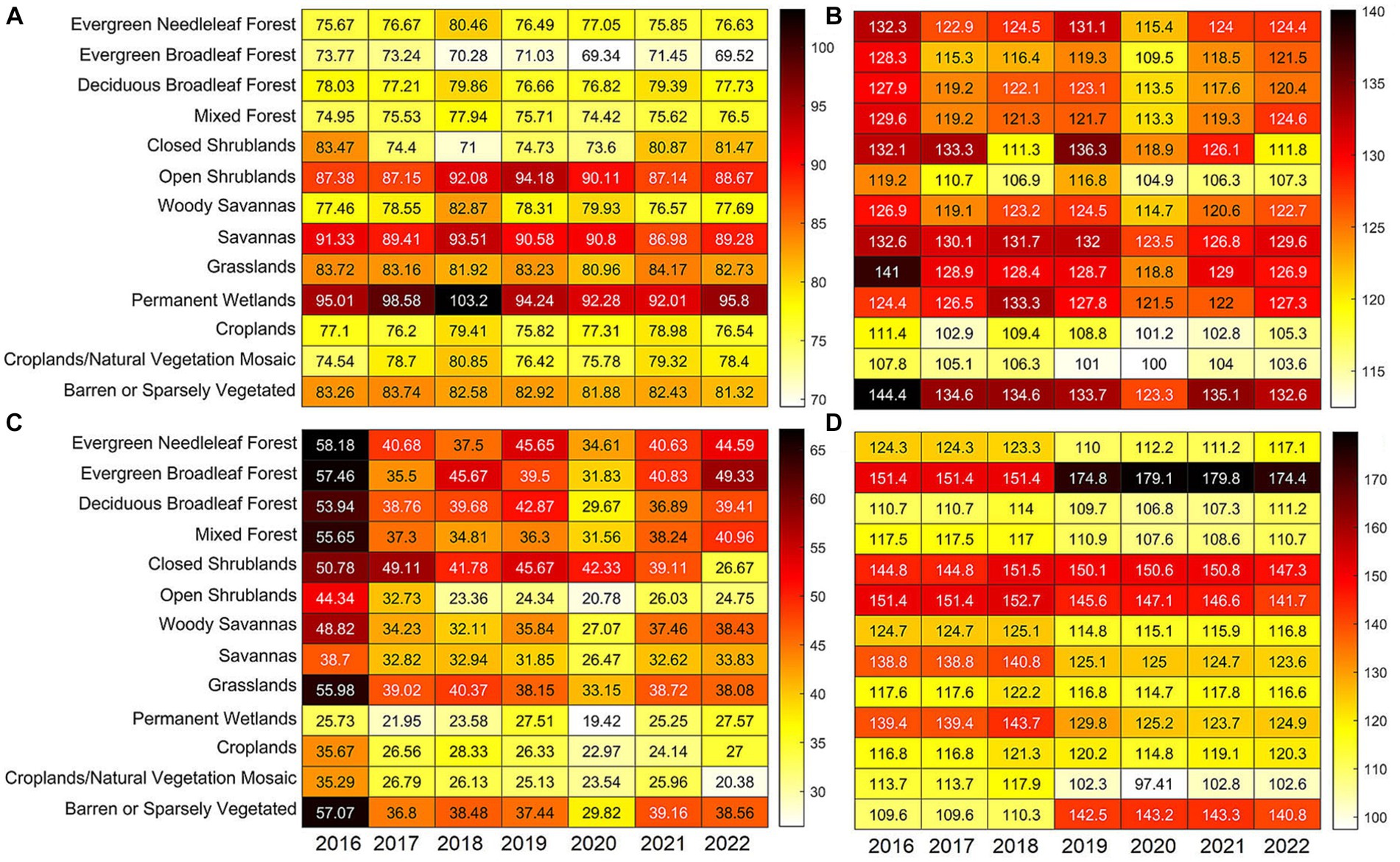
Figure 3. The heatmaps of SFT, EFT, LEF, and SOS from 2016 to 2022.

Regarding the SOS, the evergreen broadleleaf forests start the latest, followed by the shrublands. To be noticed, the woody savannas, and permanent wetlands show advance in SOS during these 7 years. There are small differences between savannas, and croplands, with an average difference of less than 10 days. Savannas are drought-tolerant plants. When the temperature reaches the conditions for savannas green-up, soil moisture is not a limiting factor anymore. Soil moisture accumulated by the process of soil F/T is getting enough to support the savannas’ growth (Xu et al., 2004). The SOS here is thus close to EFT. Regarding cropland, when the temperature reaches the conditions for vegetation emergence, an increase in soil moisture is achieved by human irrigation (Jones, 2009). Therefore, when EFT finishes, the soil moisture of this land type may advance the SOS. In contrast, there are considerable differences between EFT and SOS in broadleaf evergreen forests. This phenomenon in forests is possible because of the high demand for soil moisture.

4.3 The correlations between the SFT, EFT, LEF, and SOS in space

Correlation coefficient analysis is conducted at each grid using the seven pairs of data to test the linearity between the SFT, EFT, LEF, and SOS. Figure 4A summarizes the R-values between SFT and SOS. Consistency varies over different regions, with values ranging from −0.95 to 1. Approximately 22.6% of grids within the domain have a strong positive correlation (R ≥ 0.5); 32.3% of grids have moderate to strong negative correlation (R < -0.5), while a large majority of grids domains show a relatively weak relationship between the two records. In most of Asia, R-values remain negative. In North America, the R-values mostly show a positive correlation and are mainly concentrated in this continent’s central and southern regions. In spatial patterns, EFT and SFT differ significantly (Figure 4B). Positive correlations are distributed in eastern North America, while negative correlations are found in central North America. As for Eurasia, significant positive correlations are found only at high latitudes, while the correlations are weaker (R < 0.2) at low and middle latitudes in Eurasia. The correlation between LEF and SOS shown in Figure 4C shows a similar spatial pattern to EFT. Positive correlations occur mainly in eastern North America, and negative correlations occur at high latitudes in North America. Positive correlations occur only at high latitudes in Eurasia.

FIGURE 4

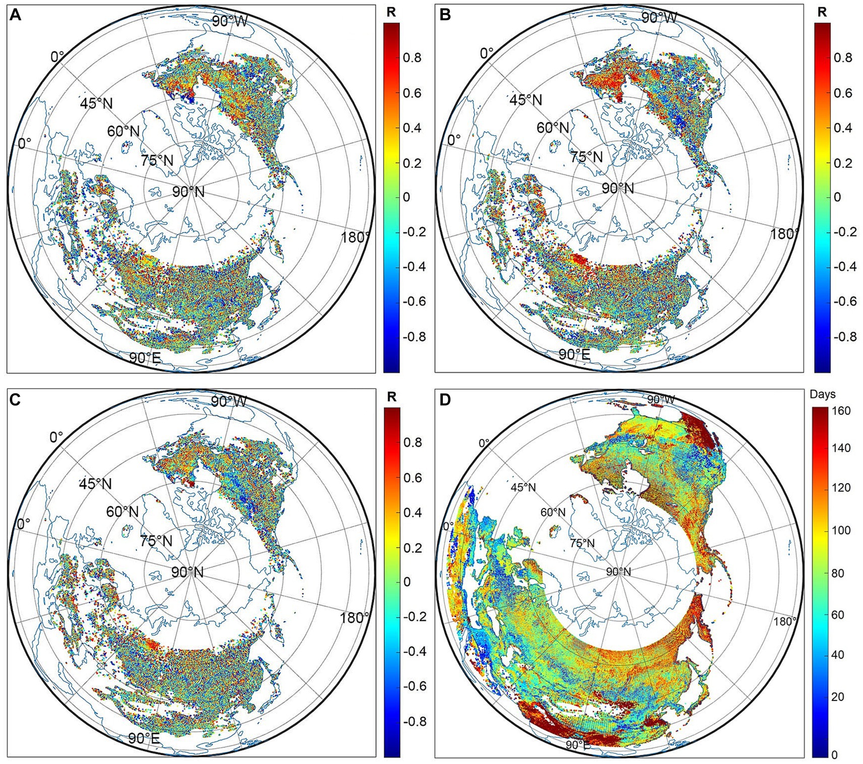
Figure 4. Comparison of R values between soil F/T state and SOS. (A) R between SFT and SOS, (B) R between EFT and SOS, and (C) R between LFT and SOS, (D) the spatial distribution of the difference between the SOS and EFT.

The difference between the SOS and EFT is obtained to further understand the drivers of uncertainty about the SOS delays (Figure 4D). Among the grids in the study area, 5.5% show a difference of less than 1 month. This suggests that environmental conditions in these areas meet the vegetation green-up soon after the soil EFT. The pixels are mainly distributed at the low-mid latitude of Europe. Approximately, SOS happens one to 2 months after the end of the soil EFT, accounting for 16.2% of grids. Around 34.9% of the whole pixels start spring onset between 2 and 4 months after soil EFT. At last, over 40% of the grids suggest even later green-up onsets after EFT by more than 120 days. As for the spatial pattern, the gaps between SOS and EFT are extremely large in two areas, i.e., the southern region of Asia, and the southwest of North America. To our knowledge, the Tibetan Plateau is located in South Asia with a relatively high altitude, i.e., > 3,000 m, resulting in cold weather (Zhao et al., 2013). As mentioned above, the strong radiation in the daytime heats the soil surface fast and leads to a long period of soil F/T. Therefore, it takes a longer time for SOS to reach the appropriate temperature after EFT. This can lead to a low temperature; thus, this area needs a long time for vegetation to green up after EFT. In the case of the northern Americas, this is a predominantly semi-arid area with grasses and shrubs. The lack of soil moisture leads to the late green-up of vegetation.

Quartile statistics (i.e., the min, maximum, median, 1st quartile, and 3rd quartile) and correlations between the SFT, EFT, LEF, and SOS are calculated for the 13 land types, as shown in the boxplot in Figure 5. Overall, the R-values of all land types range from −1 to 1. For Figure 5A, the highest median R-values for all land types ranged from −1 to 1. As depicted in Figure 5A, the highest median R-values occurred in open shrublands, closed shrublands, and permanent wetlands. The R-values for the 13 land types in Figure 5B are similar to those in Figure 5A, but slightly increased. The forest category in Figure 5C has a relatively high R-value.

FIGURE 5

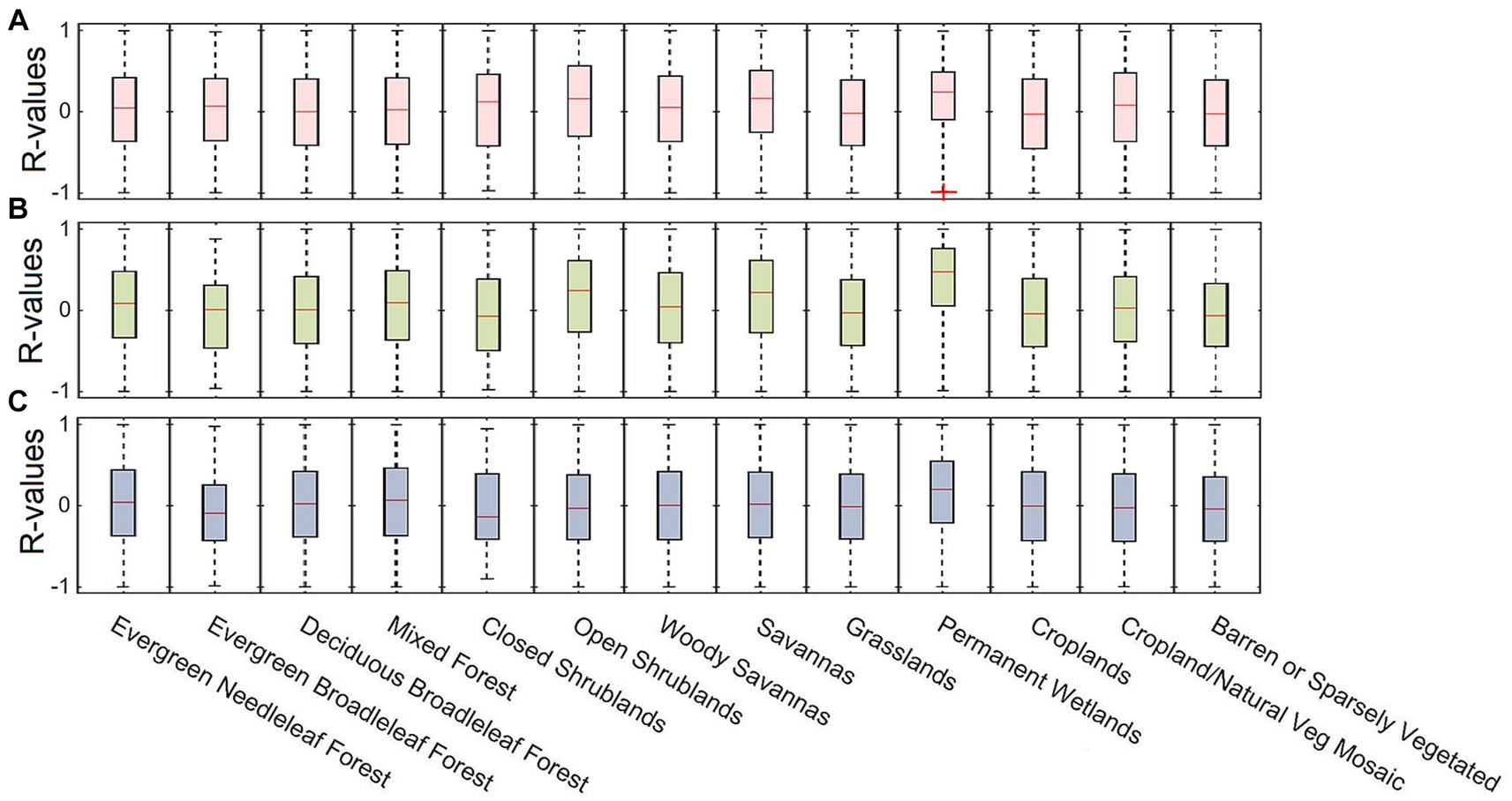
Figure 5. Boxplot of the R values for the 13 land types. (A) Boxplot between SFT and SOS, (B) boxplot between EFT and SOS, and (C) boxplot between LFT and SOS.

Figure 6 shows the average R² values of the three indexes vary with the length of LFT. Overall, these results confirm that the SFT, EFT, and LET are consistent well with the SOS, with the absolute value of R² larger than 0.2 over the entire time period. The result of EFT outperforms the other two indexes, with an increase of about 3.14% in R². As illustrated in Figure 6A, the R² values of SFT against SOS are relevant to the declining trend except for the period between 90 and 100 days. Similar to SFT, the R² values for EFT and LEF values also show a decreasing trend until the 80th period. However, the sample numbers of the length of days 80 ~ 120 are very few, which may lead to a relatively large statistical error.

FIGURE 6

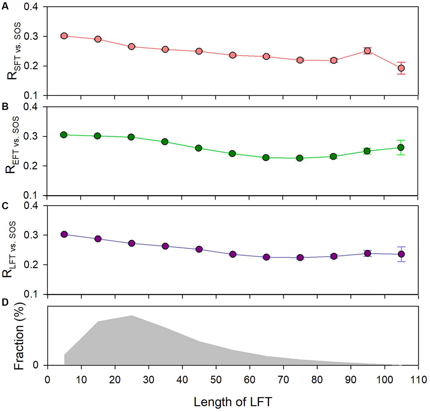
Figure 6. The average R² values of the three indexes vary with the length of LFT. (A) is the R² value of SFT vs. SOS, (B) is the R² value of EFT vs. SOS, (C) is the R² value of LET vs. SOS, and (D) is the length of LFT.

5 Discussion

As aforementioned, the soil F/T state affects the beginning of the vegetation growth period, which in turn affects net primary productivity. These biological processes would directly or indirectly influence terrestrial ecosystem carbon cycles. This research extracts three phenophases of F/T, i.e., SFT, EFT, and LFT, from winter to spring and analyzes the impact on SOS in detail. Specifically, the 3 F/T state indexes all impact SOS values, and the EFT outperforms others. It provides an interesting view of the driving mechanisms of SOS under the ongoing global warming. The results can fill the knowledge gap on the response of spring vegetation phenology to soil F/T state.

In theory, SOS should follow closely to EFT. The results confirmed this hypothesis. The process of F/T can enrich soil moisture during the period, which is beneficial for plants starting green-up onset. In particular, vegetation spring green-up onset occurs only when the temperature reaches the growing threshold and soil moisture is adequate (Wang et al., 2022). However, the above results show an overlay between the SOS and EFT. Substantially, under the dramatic global warming, soil moisture is a critical driving variable for vegetation phenology besides temperature.

Nevertheless, this study has some limitations: (1) Due to the launch of the SMAP mission being in 2015, the dataset only covers 7 years from 2016 to 2022. It is hard for us to assess the long-term variation of soil F/T state during the past several decades. (2) Here, we only take a look at the linkage between the SOS and spring soil F/T state. The vegetation activities in autumn, e.g., vegetation dormancy and the end of the growing season, can also be affected by soil F/T state. The linkage between the soil F/T state and the yearly vegetation activities will be considered in the future. (3) This study focused on exploring the impact of soil F/T state on spring vegetation phenology; other factors, e.g., soil moisture, precipitation, shortwave radiation, plant self-rhythm, and interaction, are not considered. Future work will consider more satellite data from other sources to effectively improve the accuracy of the results.

6 Conclusion

This study first comprehensively investigates the consistency of the SOS and three soil F/T state indexes, i.e., the start day of the F/T state (SFT), the end day of the F/T state (EFT), and the length of days of the F/T state (LFT) via SMAP data. Results indicate that the soil F/T state can affect the spring vegetation phenology, and the EFT outperforms the other two indexes. The main conclusion includes:

1. All 3 F/T state indexes impact SOS values, and the EFT outperforms others. The R² values between EFT and SOS gain around 3.07%.

2. The results indicate a temporal overlap between SOS and EFT. This suggests that plants begin active growth before the average temperatures reach above 0°. In addition, the spatial heterogeneity exists in the differences between SOS and EFT. The largest difference occurs in South Asia’s Tibetan Plateau and South North America’s semi-arid regions. Different driving mechanisms (e.g., altitude and soil moisture saturation) may lead to this phenomenon.

3. Moreover, for different land types, there are insignificant differences of SOS and EFT between savannas, and croplands, with an average difference of less than 10 days. In contrast, the largest differences occur in broadleaf evergreen forests.

Foeseeably, the results deepen the understanding of the implications of soil F/T state on vegetation phenology. In addition, it provides information to investigate the reasons for the nonlinear dynamics of SOS under ongoing warming.

Data availability statement

Publicly available datasets were analyzed in this study. This data can be found here: https://nsidc.org/data.

Author contributions

TY: Data curation, Funding acquisition, Methodology, Validation, Writing – original draft. NC: Writing – review & editing.

Funding

The author(s) declare financial support was received for the research, authorship, and/or publication of this article. This study was supported by the National Key Research & Development Program (2018YFA0606101), and the National Natural Science Foundation of China projects (Grant No. 42101376, 42071133).

Acknowledgments

We thank Dr. Jundong Wang for his contribution to the data processing of this paper.

Conflict of interest

The authors declare that the research was conducted in the absence of any commercial or financial relationships that could be construed as a potential conflict of interest.

Publisher’s note

All claims expressed in this article are solely those of the authors and do not necessarily represent those of their affiliated organizations, or those of the publisher, the editors and the reviewers. Any product that may be evaluated in this article, or claim that may be made by its manufacturer, is not guaranteed or endorsed by the publisher.

Supplementary material

The Supplementary material for this article can be found online at: https://www.frontiersin.org/articles/10.3389/ffgc.2023.1332734/full#supplementary-material

References

Chen, A., Meng, F., Mao, J., Ricciuto, D., and Knapp, A. K. (2022). Photosynthesis phenology, as defined by solar-induced chlorophyll fluorescence, is overestimated by vegetation indices in the extratropical northern hemisphere. Agric. For. Meteorol. 323:109027. doi: 10.1016/j.agrformet.2022.109027

CrossRef Full Text | Google Scholar

Chen, X., Liu, L., and Bartsch, A. (2019). Detecting soil freeze/thaw onsets in Alaska using SMAP and ASCAT data. Remote Sens. Environ. 220, 59–70. doi: 10.1016/j.rse.2018.10.010

CrossRef Full Text | Google Scholar

Chew, C., Lowe, S., Parazoo, N., Esterhuizen, S., Oveisgharan, S., Podest, E., et al. (2017). SMAP radar receiver measures land surface freeze/thaw state through capture of forward-scattered L-band signals. Remote Sens. Environ. 198, 333–344. doi: 10.1016/j.rse.2017.06.020

CrossRef Full Text | Google Scholar

Cong, N., Piao, S., Chen, A., Wang, X., Lin, X., Chen, S., et al. (2012). Spring vegetation green-up date in China inferred from SPOT NDVI data: a multiple model analysis. Agric. For. Meteorol. 165, 104–113. doi: 10.1016/j.agrformet.2012.06.009

CrossRef Full Text | Google Scholar

Cong, N., Wang, T., Nan, H., Ma, Y., Wang, X., Myneni, R. B., et al. (2013). Changes in satellite-derived spring vegetation green-up date and its linkage to climate in China from 1982 to 2010: a multimethod analysis. Glob. Chang. Biol. 19, 881–891. doi: 10.1111/gcb.12077

CrossRef Full Text | Google Scholar

Haboudane, D., Miller, J. R., Tremblay, N., Zarco-Tejada, P. J., and Dextraze, L. (2002). Integrated narrow-band vegetation indices for prediction of crop chlorophyll content for application to precision agriculture. Remote Sens. Environ. 81, 416–426. doi: 10.1016/S0034-4257(02)00018-4

CrossRef Full Text | Google Scholar

Jeong, S. J., Ho, C. H., Gim, H. J., and Brown, M. E. (2011). Phenology shifts at start vs. end of growing season in temperate vegetation over the northern hemisphere for the period 1982–2008. Glob. Chang. Biol. 17, 2385–2399. doi: 10.1111/j.1365-2486.2011.02397.x

CrossRef Full Text | Google Scholar

Jiang, H., Yi, Y., Zhang, W., Yang, K., and Chen, D. (2020). Sensitivity of soil freeze/thaw dynamics to environmental conditions at different spatial scales in the central Tibetan plateau. Sci. Total Environ. 734:139261. doi: 10.1016/j.scitotenv.2020.139261

PubMed Abstract | CrossRef Full Text | Google Scholar

Jones, R. A. (2009). Plant virus emergence and evolution: origins, new encounter scenarios, factors driving emergence, effects of changing world conditions, and prospects for control. Virus Res. 141, 113–130. doi: 10.1016/j.virusres.2008.07.028

CrossRef Full Text | Google Scholar

Kim, Y., Kimball, J. S., McDonald, K. C., and Glassy, J. (2010). Developing a global data record of daily landscape freeze/thaw status using satellite passive microwave remote sensing. IEEE Trans. Geosci. Remote Sens. 49, 949–960. doi: 10.1109/TGRS.2010.2070515

CrossRef Full Text | Google Scholar

Kim, Y., Kimball, J. S., Xu, X., Dunbar, R. S., Colliander, A., and Derksen, C. (2019). Global assessment of the SMAP freeze/thaw data record and regional applications for detecting spring onset and frost events. Remote Sens. 11:1317. doi: 10.3390/rs11111317

CrossRef Full Text | Google Scholar

Li, G., Zhang, M., Pei, W., Melnikov, A., Khristoforov, I., Li, R., et al. (2022). Changes in permafrost extent and active layer thickness in the northern hemisphere from 1969 to 2018. Sci. Total Environ. 804:150182. doi: 10.1016/j.scitotenv.2021.150182

PubMed Abstract | CrossRef Full Text | Google Scholar

Myneni, R. B., Keeling, C. D., Tucker, C. J., Asrar, G., and Nemani, R. R. (1997). Increased plant growth in the northern high latitudes from 1981 to 1991. Nature 386, 698–702. doi: 10.1038/386698a0

CrossRef Full Text | Google Scholar

Pardo Lara, R., Berg, A. A., Warland, J., and Tetlock, E. (2020). In situ estimates of freezing/melting point depression in agricultural soils using permittivity and temperature measurements. Water Resour. Res. 56:e2019WR026020. doi: 10.1029/2019WR026020

CrossRef Full Text | Google Scholar

Piao, S., Fang, J., Zhou, L., Ciais, P., and Zhu, B. (2006). Variations in satellite-derived phenology in China’s temperate vegetation. Glob. Chang. Biol. 12, 672–685. doi: 10.1111/j.1365-2486.2006.01123.x

CrossRef Full Text | Google Scholar

Piao, S., Liu, Z., Wang, T., Peng, S., Ciais, P., Huang, M., et al. (2017). Weakening temperature control on the interannual variations of spring carbon uptake across northern lands. Nat. Clim. Chang. 7, 359–363. doi: 10.1038/nclimate3277

CrossRef Full Text | Google Scholar

Piao, S., Tan, J., Chen, A., Fu, Y. H., Ciais, P., Liu, Q., et al. (2015). Leaf onset in the northern hemisphere triggered by daytime temperature. Nat. Commun. 6:6911. doi: 10.1038/ncomms7911

PubMed Abstract | CrossRef Full Text | Google Scholar

Rowlandson, T. L., Berg, A. A., Roy, A., Kim, E., Lara, R. P., Powers, J., et al. (2018). Capturing agricultural soil freeze/thaw state through remote sensing and ground observations: a soil freeze/thaw validation campaign. Remote Sens. Environ. 211, 59–70. doi: 10.1016/j.rse.2018.04.003

CrossRef Full Text | Google Scholar

Schwartz, M. D. (1998). Green-wave phenology. Nature 394, 839–840. doi: 10.1038/29670

CrossRef Full Text | Google Scholar

Shen, M., Piao, S., Cong, N., Zhang, G., and Jassens, I. A. (2015). Precipitation impacts on vegetation spring phenology on the T ibetan P lateau. Glob. Chang. Biol. 21, 3647–3656. doi: 10.1111/gcb.12961

CrossRef Full Text | Google Scholar

Tucker, C. J., Pinzon, J. E., Brown, M. E., Slayback, D. A., Pak, E. W., Mahoney, R., et al. (2005). An extended AVHRR 8-km NDVI dataset compatible with MODIS and SPOT vegetation NDVI data. Int. J. Remote Sens. 26, 4485–4498. doi: 10.1080/01431160500168686

CrossRef Full Text | Google Scholar

Wang, C., Yang, K., and Zhang, F. (2020). Impacts of soil freeze–thaw process and snow melting over Tibetan plateau on Asian summer monsoon system: a review and perspective. Front. Earth Sci. 8:133. doi: 10.3389/feart.2020.00133

CrossRef Full Text | Google Scholar

Wang, J., and Liu, D. (2022). Vegetation green-up date is more sensitive to permafrost degradation than climate change in spring across the northern permafrost region. Glob. Chang. Biol. 28, 1569–1582. doi: 10.1111/gcb.16011

PubMed Abstract | CrossRef Full Text | Google Scholar

White, M. A., de Beurs, K. M., Didan, K., Inouye, D. W., Richardson, A. D., Jensen, O. P., et al. (2009). Intercomparison, interpretation, and assessment of spring phenology in North America estimated from remote sensing for 1982–2006. Glob. Chang. Biol. 15, 2335–2359. doi: 10.1111/j.1365-2486.2009.01910.x

CrossRef Full Text | Google Scholar

Xie, H. Y., Jiang, X. W., Tan, S. C., Wan, L., Wang, X. S., Liang, S. H., et al. (2021). Interaction of soil water and groundwater during the freezing–thawing cycle: field observations and numerical modeling. Hydrol. Earth Syst. Sci. 25, 4243–4257. doi: 10.5194/hess-25-4243-2021

CrossRef Full Text | Google Scholar

Xu, L., Baldocchi, D. D., and Tang, J. (2004). How soil moisture, rain pulses, and growth alter the response of ecosystem respiration to temperature. Glob. Biogeochem. Cycles 18:GB4002. doi: 10.1029/2004GB002281

CrossRef Full Text | Google Scholar

Yang, K., and Wang, C. (2019). Water storage effect of soil freeze-thaw process and its impacts on soil hydro-thermal regime variations. Agric. For. Meteorol. 265, 280–294. doi: 10.1016/j.agrformet.2018.11.011

CrossRef Full Text | Google Scholar

Yu, H., Luedeling, E., and Xu, J. (2010). Winter and spring warming result in delayed spring phenology on the Tibetan plateau. Proc. Natl. Acad. Sci. 107, 22151–22156. doi: 10.1073/pnas.1012490107

PubMed Abstract | CrossRef Full Text | Google Scholar

Zhang, X., Friedl, M. A., Schaaf, C. B., Strahler, A. H., Hodges, J. C., Gao, F., et al. (2003). Monitoring vegetation phenology using MODIS. Remote Sens. Environ. 84, 471–475. doi: 10.1016/S0034-4257(02)00135-9

CrossRef Full Text | Google Scholar

Zhao, Z., Cao, J., Shen, Z., Xu, B., Zhu, C., Chen, L. W. A., et al. (2013). Aerosol particles at a high-altitude site on the southeast Tibetan plateau, China: implications for pollution transport from South Asia. J. Geophys. Res. Atmos. 118, 11–360. doi: 10.1002/jgrd.50599

CrossRef Full Text | Google Scholar

Zhou, L., Tucker, C. J., Kaufmann, R. K., Slayback, D., Shabanov, N. V., and Myneni, R. B. (2001). Variations in northern vegetation activity inferred from satellite data of vegetation index during 1981 to 1999[J]. J. Geophys. Res. Atmos. 106, 20069–20083. doi: 10.1029/2000JD000115

CrossRef Full Text | Google Scholar