 Xiaoning Li1,2
 Yuheng Zhu
- 1College of Computer Science and Technology, Jilin University, Changchun, China
- 2College of Computer Science and Technology, Changchun Normal University, Changchun, China
Soil temperature (ST) is a crucial parameter in Earth system science. Accurate ST predictions provide invaluable insights; however, the “black box” nature of many deep learning approaches limits their interpretability. In this study, we present the Encoder-Decoder Model with Interpretable Spatio-Temporal Component (ISDNM) to enhance both ST prediction accuracy and its spatio-temporal interpretability. The ISDNM combines a CNN-encoder-decoder and an LSTM-encoder-decoder to improve spatio-temporal feature representation. It further uses linear regression and Uniform Manifold Approximation and Projection (UMAP) techniques for clearer spatio-temporal visualization of ST. The results show that the ISDNM model had the highest R2 ranging from 0.886 to 0.963 and the lowest RMSE ranging from 6.086 m3/m3 to 12.533 m3/m3 for different climate regions, and demonstrated superior performance than all the other DL models like CNN, LSTM, ConvLSTM models. The predictable component highlighted the remarkable similarity between Medium fine and Very fine soils in China. Additional, May and November emerged as crucial months, acting as inflection points in the annual ST cycle, shaping ISDNM model’s prediction capabilities.
1 Introduction
Soil temperature (ST) has been recognized as a vital element of the Essential Climate Variables by the Global Observing System for Climate (GCOS, 2016). It is integral to a plethora of ecosystem processes and functions (Yan et al., 2018). Moreover, ST exerts substantial influence across diverse disciplines, including meteorology (Sanikhani et al., 2018; Feng et al., 2019), agriculture (Cornu et al., 2016; Kim et al., 2016; Zhang et al., 2021), environmental studies (Yang et al., 2019; Xu et al., 2021; Wei et al., 2023), and climate change research (Li et al., 2022a; Ran et al., 2023). Accurate predictions of ST can aid in mitigating soil erosion, optimizing water utilization during irrigation, and enhancing grain yields (Karandish and Shahnazari, 2016; Bodić et al., 2018). Historically, the primary approach to understanding ST has been through process-based models, which operate on control equation feedback tied to intricate land-atmosphere mechanisms (Kalakuntla et al., 2013), such as the land-surface data assimilation method (Henderson-Sellers et al., 1993). However, these models’ computational demands, coupled with uncertainties in physical drivers and potential oversights in key processes, contribute to prediction ambiguities (Reichstein et al., 2019).
In more recent times, data-driven models have garnered traction in Earth science applications (Reichstein et al., 2019), with estimations spanning a range of meteorological variables, including atmospheric and dew point temperatures, precipitation, solar radiation, and soil moisture (Kisi et al., 2013; Cobaner et al., 2014; Kisi and Sanikhani, 2015; Mohammadi et al., 2016; Li Q. et al., 2020; Li et al., 2021, 2022a,b).
Conventional machine learning (ML) models, such as Multi-Layer Perceptron (MLP), Back Propagation Neural Networks (BPNN), Extreme Learning Machine (ELM), Generalized Regression Neural Networks (GRNN), and Radial Basis Neural Networks (RBNN), have risen in prominence for ST prediction. They adeptly map the intricate, nonlinear dynamics between ST and selected influencing factors. For instance, Tabari et al. (2011, 2015) leveraged the MLP model for daily ST prediction in Iran, noting the significance of ST memory for enhancing extended ST predictions. Yin et al. (2023) predicted changes in lake boundaries based on U-net and spatial transformation network. Similarly, studies by Kisi et al. (2013), Sanikhani et al. (2018), and Feng et al. (2019) showcased the merits of RBNN, ELM, and BPNN, respectively, in ST estimations across different contexts. The fusion of ML models with other techniques has been spotlighted as a promising avenue, delivering enhanced accuracy in both short-term and long-term ST predictions (Mehdizadeh et al., 2020). Nevertheless, there remains a window of opportunity for refinement and innovation in this domain, as alluded to by Yan et al. (2020).
ST prediction has been notably augmented by the implementation of deep learning (DL) methods (Li L. et al., 2020; Li Q. et al., 2020; Li et al., 2021, 2022a,b). One classical DL method is the Long Short-term Memory (LSTM) network (Hochreiter and Schmidhuber, 1997), adept at utilizing sequential data. With its unique capability to use prior outputs as inputs and preserve this information through memory gates, LSTMs have gained prominence in ST prediction. For instance, Li Q. et al. (2020) employed multi-channel LSTM with lagged ST data, revealing its proficiency in capturing both long-term and short-term ST behaviors.
Convolutional Neural Networks (CNN) (LeCun et al., 1989), another DL archetype, excel in memory efficiency through their convolutional structure. With components like local perception fields, weight sharing, and pooling layers, CNNs mitigate model overfitting. Their application in ST prediction, such as by Hao et al. (2020), has validated their effectiveness, especially when utilizing historical ST data.
Although deep learning models are widely used in ST prediction, Yet, capturing the nuanced spatio-temporal variations of ST remains challenging. Factors influencing ST vary temporally and spatially, and these variations often interplay (Zhao et al., 2013; Li et al., 2022a). Furthermore, another lingering concern with DL methods, however, is their “black box” nature, often eliciting skepticism due to over-parameterization and unclear mechanisms (Li et al., 2022a). Advancing DL model interpretability is, thus, also a prime challenge (Reichstein et al., 2019).
Addressing these, the model first incorporated an encoder-decoder structure, known to boost deep learning efficacy (Cho et al., 2014; Shang and Luo, 2021). Furthermore, our Interpretable Spatio-Temporal Deep Network Model (ISDNM) synergized the strengths of both CNN and LSTM by melding the CNN-encoder-decoder with the LSTM-encoder-decoder. While the LSTM captures temporal nuances, the CNN is more attuned to spatial variations.
Second, our model incorporated spatio-temporal interpretable components and grounded the learning process in physical knowledge, analyzing the interactions between influencing factors and ST variations.
In essence, ISDNM was designed to not only enhance ST prediction but also to clarify its learning mechanisms. Comprising a prediction component and an interpretable component, it marries the accuracy of capturing spatio-temporal ST variations with heightened model interpretability. Our key contributions include:
1. A cutting-edge fusion model elevating predictive performance.
2. An innovative interpretable component offering spatio-temporal insights.
3. Benchmarking of ISDNM against CNN, LSTM, and ConvLSTM, underscoring its superior predictive prowess.
2 Materials and methods
The ISDNM model was introduced to enhance the accuracy of ST prediction and to provide a clear interpretation of the model’s operation. The selection of algorithms was based on their suitability for handling the complex spatio-temporal patterns in our dataset. The CNN and LSTM architectures were chosen for their proven capabilities in capturing spatial and temporal dependencies, respectively, which have been demonstrated in previous studies related to soil temperature prediction (Li L. et al., 2020; Li Q. et al., 2020; Li et al., 2021, 2022b). The integration of these models in our Interpretable Spatio-Temporal Deep Network Model (ISDNM) allowed us to exploit the synergies between these techniques, enhancing the model’s ability to extract nuanced spatio-temporal features. As illustrated in Figure 1, the model is bifurcated into: (i) the predictive component and (ii) the interpretable component. The former is dedicated to extracting both spatio-temporal and time-variant features of ST, thereby boosting predictive accuracy. In contrast, the interpretable component, which comprises a linear regression model paired with Uniform Manifold Approximation and Projection (UMAP), seeks to furnish spatio-temporal interpretive results for ST.
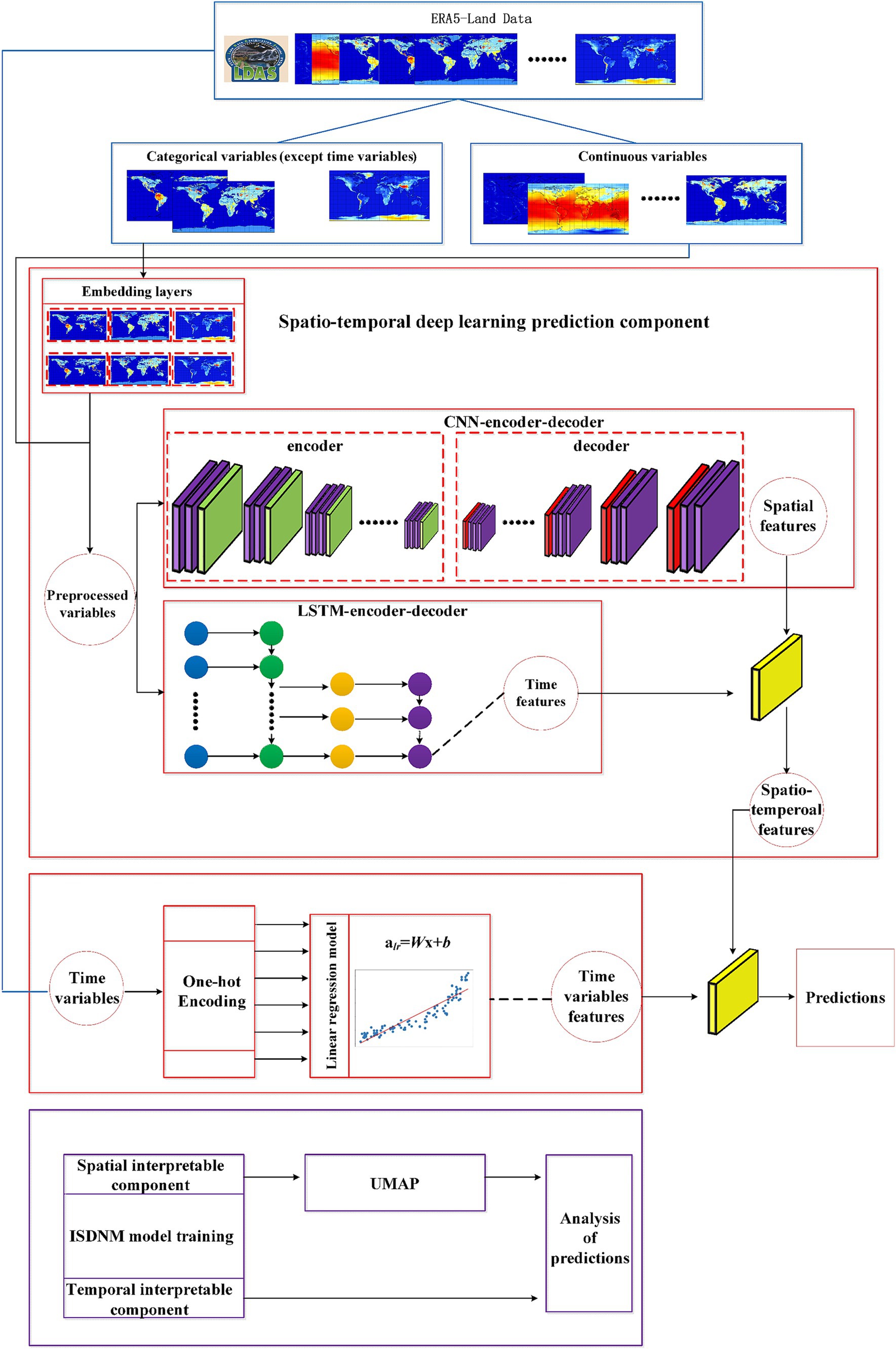
Figure 1. Technology roadmap based on interpretable spatio-temporal deep learning model.
2.1 Data
For testing DL models in ST prediction, the model adopted the ERA-5 data product. Utilizing 36KM spatial resolution data as our input, the new structure not only expedited the model’s validation but also earmarked future exploration at finer spatial resolutions. Key meteorological variables incorporated include soil moisture (SM), total precipitation (TP), 2 m-height wind speed (Wind), 2 m-height air temperature (AT), short-wave radiation (SW), long-wave radiation (LW), and surface pressure (SP). These factors were highlighted for their significance in ST prediction by Li et al. (2022a). The dataset was divided into training, testing, and validation sets, typically using a 4:1:1 split ratio. The exact percentages were chosen to strike a balance between having a sufficiently large training dataset for model learning and ensuring rigorous evaluation on unseen data through testing and cross-validation. These percentages were selected based on prior literature and experimental validation to ensure the robustness and reliability of our results (Li L. et al., 2020; Li Q. et al., 2020; Li et al., 2021, 2022b). Specifically, the data, spanning from 2015 to 2020, carries a temporal resolution of a day. The span between 2015 and 2018 was earmarked for training, 2019 for validation, and 2020 for testing. The geographical scope encompassed China, with longitudes ranging from 73°33′E to 135°05′E and latitudes from 3°51’N to 53°33’N, offering a comprehensive national-scale testbed for ST prediction. The selection of the entire China as the case study was driven by several considerations. Firstly, China offers a vast and diverse geographical landscape with varied climate patterns (Beck et al., 2018), providing an ideal context to explore intricate spatio-temporal variations. Additionally, the nationwide scale of the study allowed for meaningful insights applicable to a wide array of environmental and agricultural planning scenarios. By opting for a nationwide scope, the research aims to contribute valuable knowledge that can inform policymakers and stakeholders at a national level, providing insights with broad applicability and relevance. It is worth to note that the variables are bifurcated into continuous and categorical types, the normalization was exclusive to continuous variables, with categorical ones remaining unchanged, as elaborated in Section 2.3.
2.2 Data preprocessing
Data was subjected to three preprocessing techniques: (i) Min-Max normalization, (ii) one-hot encoding, and (iii) entity embedding. These methodologies are oriented toward expediting model training. Primarily, Min-Max normalization is a tool to rescale data such that each element across the data spectrum is represented as a value between 0 and 1. The formula for Min-Max normalization is as follows:
The normalized value, denoted by Xnorm is defined based on Xmax and Xmin, which, respectively, represent the data’s maximum and minimum values. Further, our model employs one-hot encoding, a method that represents categorical month variables (January through December) with a binary string. In this representation, one bit is set to 1 while the remaining bits are 0. Entity embedding, on the other hand, is leveraged to streamline data, specifically by turning categorical features into continuous ones using word embedding techniques.
2.3 Predictable component
To begin with, time variables are constructed using one-hot encoding, with months serving as the foundational time unit. For instance, if the current time variable corresponds to March, the third bit in the 12-bit encoded feature is set to 1, while all other bits are 0. The CNN-encoder-decoder model and LSTM-encoder-decoder model are tasked with extracting spatial and temporal features, respectively. Following their extraction, these features are amalgamated via a fully connected layer, yielding a comprehensive spatio-temporal feature. Post-training, the model adeptly extracts both time variable features and the combined spatio-temporal feature, leading to enhanced predictive accuracy.
The predictive component comprises the CNN-encoder-decoder model and the LSTM-encoder-decoder model. The primary role of the CNN-encoder-decoder model is to delineate spatial characteristics of ST. Initial steps involve segmenting the accumulated data into continuous and categorical variables. The spatial interpretability component primarily processes continuous variables like SM, TP, Wind, AT, SW, LW, and SP, alongside categorical non-temporal variables such as soil type and vegetation type. These variables undergo preprocessing using the entity embedding method and Z-score normalization, respectively. Subsequent to this preprocessing, the normalized continuous features and the categorical features are forwarded to the spatio-temporal deep learning model. This model, in turn, concurrently interprets both the temporal and spatial nuances of ST.
The time variable chiefly undergoes processing in the linear regression prediction model, facilitated by one-hot encoding (similar to the encoding described above for months). These encoded features are then channeled into a linear regression model, yielding characteristics specific to the time variable. Both temporal and spatial features, along with time variable characteristics, are integrated using a weighted sum approach within a fully connected layer. The combined features are then co-trained. The calculations are structured as follows:
Where Y is the predicted value, is the output weight of deep learning prediction component, is the output weight of linear regression prediction component, and b is the bias term. The predicted value Y of ST and the actual value Y’ of ST will be transferred to the loss function training prediction model.
2.3.1 LSTM-encoder-decoder
LSTM-encoder-decoder mainly extracts the temporal dimensional feature of ST, and the core part also includes an encoding network and a corresponding decoding network. The model encoder the previous states of ST, and decoder the current ST for ST temporal. The ST at the previous time and the current time state of the decoder to obtain the ST temporal feature at this time.
The model uses the semantic coding vector C at each time, the ST at the previous time and the current time state of the decoder to obtain the ST time characteristic feature at this time through the full connection layer function g, and the calculation is as follows:
The semantic coding vector at each time is obtained by weighting the hidden vector at each time of the encoder, indicating that the influencing factors of ST may be different at each time. is calculated as follows:
In equation 4, represents the hidden vector at time I in the encoder, refers to the weight of the hidden vector at each time in the encoder, and are calculated as follows:
In equation 5, is calculated from the state of the decoder at the previous time and the hidden vector hi of the encoder at the current time, as follows:
In equation 6, U, V and W represent the parameters of the model, and tanh refers to the hyperbolic tangent activation function; the current time state of the decoder is calculated as follows:
In equation 7, refers to the actual value of ST at time j-1, and f represents the decoder network model.
2.3.2 The CNN-encoder-decoder
The CNN-encoder-decoder is specifically designed to extract the spatial features of ST. This model boasts six convolution kernels. Its architecture is bifurcated into an encoding network and a complementary decoding network.
The encoding segment comprises a convolutional layer, a batch normalization layer, a rectified linear unit (ReLU) for activation, and a pooling layer. The initial three convolution kernels play a pivotal role in reducing resolution. Conversely, the decoding section is outfitted with an upsampling layer, a convolutional layer, a batch normalization layer and a ReLU. It’s worth highlighting that the last three convolution kernels within the decoder serve to extrapolate the spatial feature of ST. This is achieved by restoring the low-resolution encoded feature map of ST to its original input resolution.
2.4 Iinterpretable component
The primary objective of the spatial component is to elucidate the spatial correlations inherent in ST. At its heart, this component is equipped with an embedding layer and UMAP. When grappling with categorical variables, the model have opted for the entity embedding approach as proposed by Guo and Berkhahn (2016). Their research underscored the efficacy of this method over traditional one-hot encoding. The advantage being, it sidesteps the pitfalls of data sparsity post-encoding, which can detrimentally impact prediction model accuracy.
UMAP, standing on the foundational principles outlined by McInnes et al. (2018), leverages local manifold approximations. These approximations are meticulously stitched together, utilizing their local fuzzy simplicial set representations. This methodical process constructs a topological representation of high-dimensional data. Furthermore, a parallel process can craft an equivalent topological representation, culminating in the minimization of the cross-entropy between the two representations. In practice, UMAP is adept at condensing the embedded vectors into a three-dimensional space, enabling a vivid visualization of ST’s spatial correlations.
In its operational phase, UMAP shrinks the embedded vector to a three-dimensional realm. This aids in calculating the cosine distance between disparate variables, serving as a benchmark to discern inter-variable correlations. The pertinent calculations are articulated as follows:
Let Xi and Yi denote eigenvectors of length N. A smaller value indicates a heightened correlation between the two eigenvectors. For instance, when analyzing the spatial influence of ST on terrain, one can examine it within a three-dimensional space. If two specific terrain eigenvectors are proximate within this space, it suggests that the ST of the two terrains significantly influences each other.
Furthermore, by extracting the weights from the linear regression model, the model can directly gauge the contribution of each individual value within a variable. To illustrate, if the ‘month’was considered as the temporal variable, it can shed light on the monthly impact on ST. A higher absolute weight value signifies that a particular month exerts a considerable influence on the ST.
3 Results
The model experimented with various DL architectures to forecast ST. For evaluation, metrics like R2, RMSE and MAE were reported (Willmott and Matsuura, 2005; Hyndman and Koehler, 2006). The formula for calculating RMSE, MAE and R2 is as follows:
where yi is the observed variables of the i-th time steps, ŷi is the predicted variables of the i-th time steps obtained by predictive models, and −yi is the average value of the observed variables.
As shown in Table 1, the ISDNM outperforms standard DL methods in terms of RMSE, MAE and R2.
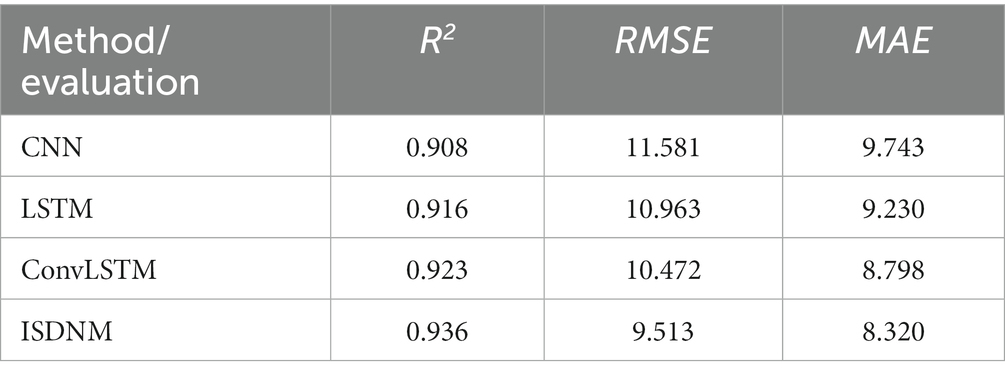
Table 1. Comparison of the performance of different models (including CNN, LSTM, ConvLSTM, and ISDNM).
3.1 Non-linear relationship between ST and meteorological factors
Prior research underscores the significance of meteorological variables in predicting ST (Cornu et al., 2016; Kim et al., 2016; Sanikhani et al., 2018; Feng et al., 2019). Our exploration first delves into the nonlinear associations between ST and several meteorological factors. The left and middle columns of Figure 2 present the spatial distribution and histograms of selected meteorological variables, such as precipitation, wind speed, and soil type, among others. The right column of the figure depicts relationships between ST and these variables, as modeled by the Generalized Additive Model (GAM).
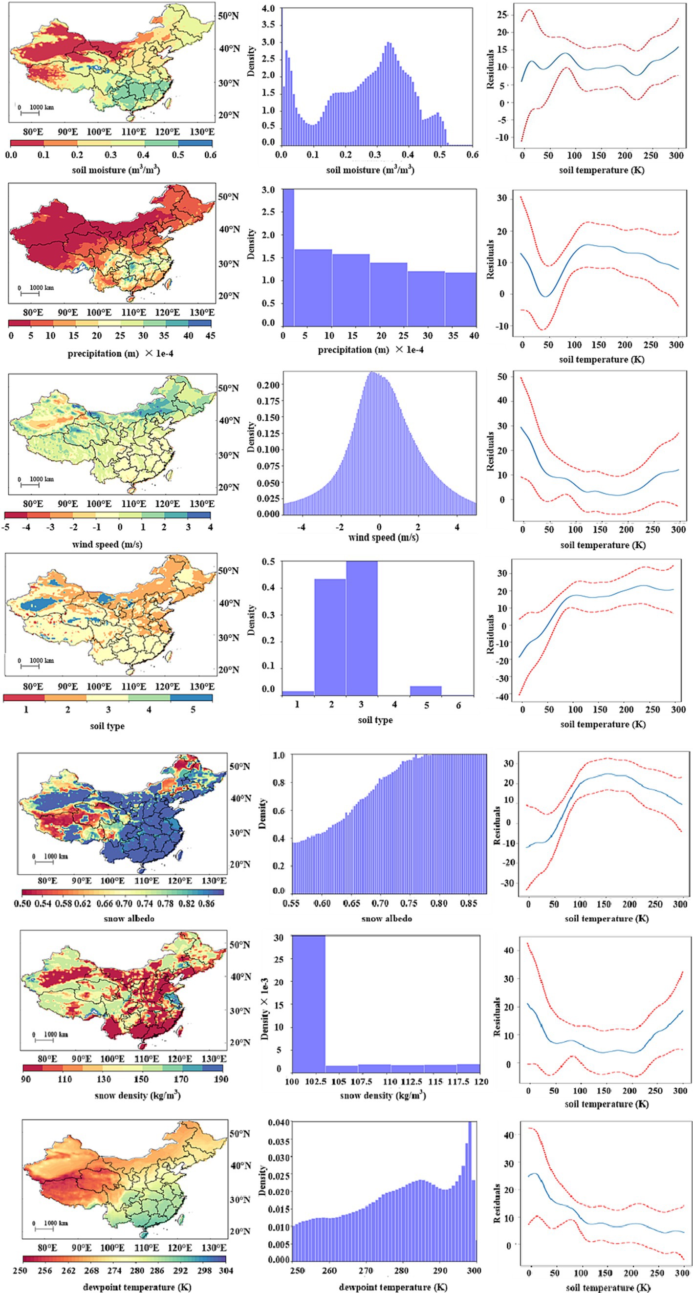
Figure 2. RMSE, R2 and DELTA comparison between the ISDNM model and other models.
From Table 1 and Figure 3, it can observe that northern China experiences lower precipitation levels. Regions with substantial rainfall are predominantly located in the middle and lower reaches of the Yangtze River plain, with the precipitation values of north China mainly ranging from 0 m to 0.0005 m. Wind speed is notably higher in northern areas, especially central Inner Mongolia, while other regions record speeds mainly between 0 m/s and 1 m/s.
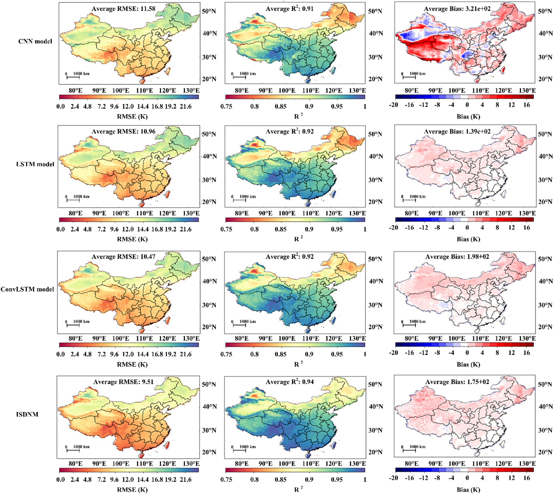
Figure 3. Spatial distribution of variables (left column), descriptive statistics (middle column) GAM plot (right column). Shaded areas in the GAM plot indicate 95% confidence intervals. The value of p is 1.11e-16***. The area enclosed by two red lines in the GAM plot indicates the 95% confidence interval, and the Y-axis indicates the effective degrees of freedom for covariates and smoothing. The *** after each value of p indicates the 99% confidence interval of the fit (soil type 1: coarse; 2: medium; 3: medium-fine; 4: fine; 5: very fine; 6: organic; 7: tropical organic).
The Southern part of China mainly comprises medium to fine soils, while northern regions predominantly have coarse soils. Deserted regions in northwest China and certain parts of Inner Mongolia exhibit very fine soil types.
In warmer areas, such as south and central China and Xinjiang province, snow albedo primarily lies between 0.8 and 0.9. Colder regions like Heilongjiang province, Jilin province, and Tibet province see values around 0.5. Snow density distribution mirrors snow albedo, with warmer areas having lower values and cold regions, especially the northeast and Inner Mongolia, registering higher figures.
Soil moisture measurements in areas like Xinjiang, northern Tibet, and western Inner Mongolia hover around 0.1. In contrast, regions around the Yangtze River Plain show a value close to 0.5. Central and northeastern China typically record values between 0.3 and 0.4.
Lastly, dew point temperature exhibits distinctive characteristics: high-altitude areas such as Tibet report temperatures between 250 K and 260 K. In regions without significant altitude variations, the dew point temperature relates directly to ambient temperatures: colder environments have lower dew point temperatures and vice versa.
3.2 Overall performance of CNN, LSTM, CONVLSTM and ISDNM
In the ISDNM model, an LSTM cell with a hidden size of 512 was implemented. The training was configured for 100 epochs with a learning rate of 0.001. A maximum timestep of 7 was set, and a batch size of 128 was determined. The mean squared error served as the loss function, and the Adam optimization technique was employed. The LSTM, CNN, and ConvLSTM models shared identical parameters with ISDNM. Through rigorous testing, these parameter choices consistently outperformed alternatives. Able 1 provides a comparative performance analysis. ISDNM stood out with the highest ST predictive accuracy, achieving R2 = 0.936, RMSE of 9.513, and MAE of 8.320. Amongst all deep learning models tested, only ConvLSTM came close to the ISDNM’s performance, while CNN was the least effective.
Figure 2 visualizes the performance metrics of CNN, LSTM, ConvLSTM, and ISDNM models over the testing period. While most of China recorded an RMSE below 12, the northeastern and northwestern regions showcased patches with higher RMSE and lower R2 values. This could be attributed to these regions experiencing significant ST variations.
To dissect these anomalies, seasonal performances using the ISDNM model were analyzed. Figure 4 elucidates the season-wise performance. The metrics considered included RMSE, R2, lag R, and standard deviation (SD). It became evident that both summer and winter seasons were challenging periods, displaying increased RMSE and diminished R2 values. Higher lag R and elevated SD values likely misled the model, causing dips in predictive accuracy. Both northeastern and northwestern regions manifested these heightened values throughout the year, particularly during summer and winter, explaining their reduced model performance.
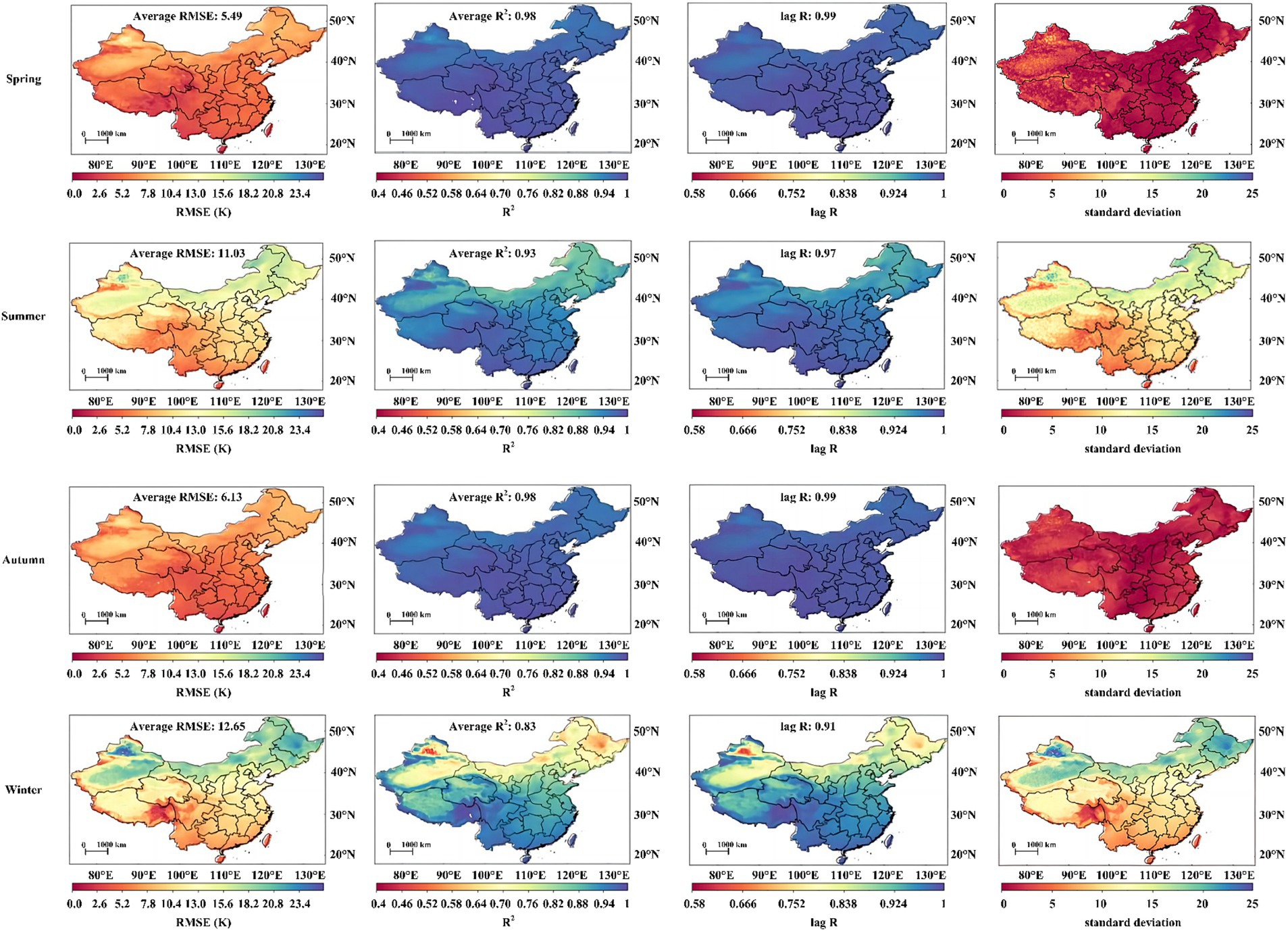
Figure 4. The RMSE, R2, lag R and SD of ISDNM for different season.
3.3 Sensitive analysis for different input data
SM influences the soil’s water balance and subsequently affects ST, a relationship echoed in the findings of Zheng et al. (1993). External factors like precipitation, wind speed, and air temperature (AT) play pivotal roles in modulating ST. For instance, wind speed impacts evapotranspiration rates which, in turn, influence ST (Valipour, 2015). Furthermore, SW and LW absorbed by soil also affect ST, as described by Ronda and Bosveld (2009). Considering these interdependencies, SM, TP, Wind, AT, SW, LW, SP, SOILT, and THV were selected as foundational input variables. Table 2 presents the performances of CONVLSTM and ISDNM models across ten different input combinations, mirroring the methodology of prior research like (Li et al., 2022a).
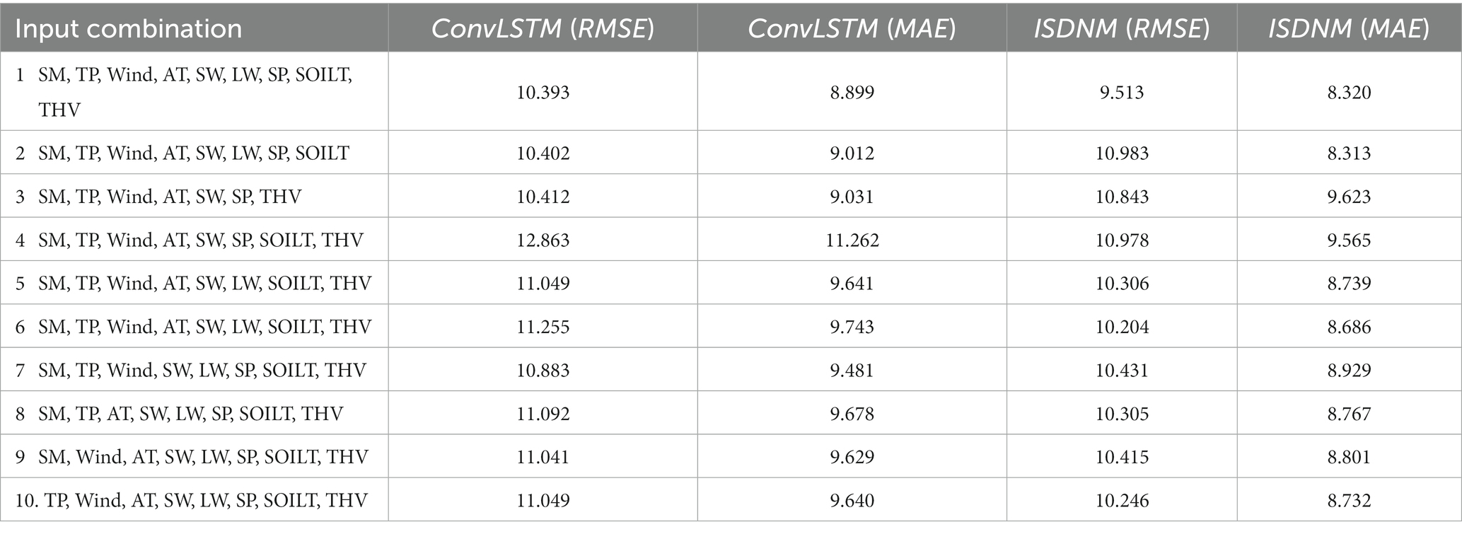
Table 2. Comparison of the performance of different input combination.
While combination 1 utilized all basic input variables, combinations 2 through 10 adopted various permutations by omitting individual inputs. Notably, optimal results emerged when using all basic inputs. As per Table 2, the ISDNM model consistently surpassed the CONVLSTM in accuracy across all input combinations. While the omission of any foundational variable typically impacted model performance, certain combinations, such as 1, 2, and 3, still displayed comparable results.
3.4 Impact across different climate zones
Evaluating ST based on climate zones can offer nuanced insights into climate change dynamics (Li et al., 2021). Referencing the Köppen-Geiger classification (Beck et al., 2018), the ST prediction performance across China’s diverse climate zones were assessed. Figure 5 categorizes China into eight distinct climate zones, and Table 3 presents their respective metric averages. The arid desert climate zone, primarily in Xinjiang, exhibited top-tier performance, likely due to its pronounced ST memory as reflected by a high lag R value (0.983). Conversely, the tropical monsoon/savannah climate zone struggled, potentially due to its limited sample size (0.2%) and a lower lag R (0.934). A similar trend was observed in the cold-no-dry season climate zone. The cold-dry-winter zone, encompassing 25.8% of the sample and centered in North-East and Central China, yielded commendable results, perhaps due to the region’s high lag R correlation with ST. Overall, a strong correlation between ST’s lag R and model prediction performance was unmistakable.
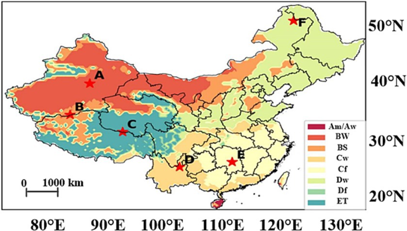
Figure 5. The Köppen-Geiger climate region map of China.
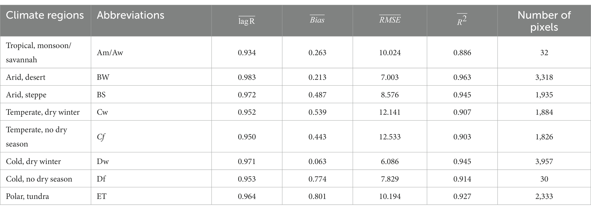
Table 3. Mean value of different metric of different climate regions, the lagged correlation of ST (lagged R), the Bias (K), root-mean-square error (RMSE, K) and R-square of the ISDNM, and number of pixels.
3.5 Improvements in model performance
Figure 6 illustrates the R2, RMSE, and bias values for the CNN, LSTM, ConvLSTM, and ISDNM models. Evidently, the ISDNM model emerges as the premier deep learning model for ST prediction. This is discernible from its near-zero bias, its superior average R2 value which oscillates between 0.886 and 0.963, and its unrivaled minimal mean RMSE, which ranges from 6.086 to 12.533. The ISDNM’s superior performance is consistent across all eight climate zones in China. However, its distinct advantage is somewhat less pronounced in the tropical monsoon/savannah and cold, non-dry season zones, possibly due to limited sample sizes within these regions.
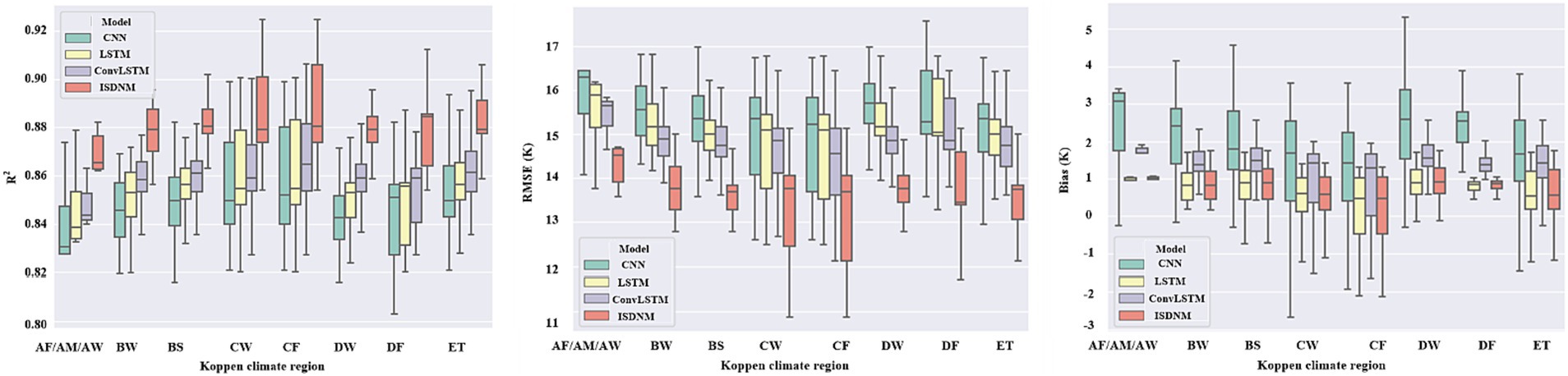
Figure 6. The box plots of the R square, RMSE and bias.
3.6 Spatio-temporal feature extraction using ISDNM
Figure 7 showcases the cosine distances of ST values across various soil types. An interesting observation is the proximity in cosine distance values between soil types 4 (Medium fine) and 5 (Very fine) in China. The minimized distance suggests that these two soil types share analogous features when analyzed by the model. This resemblance is likely because Medium fine and Very fine soils exhibit similar energy and water exchange characteristics compared to other soil types (Hulugalle et al., 2001; Yuan et al., 2023). The observation that identical soil types tend to have harmonized soil moisture exchanges validates our choice of using soil moisture as an essential covariate to characterize ST.
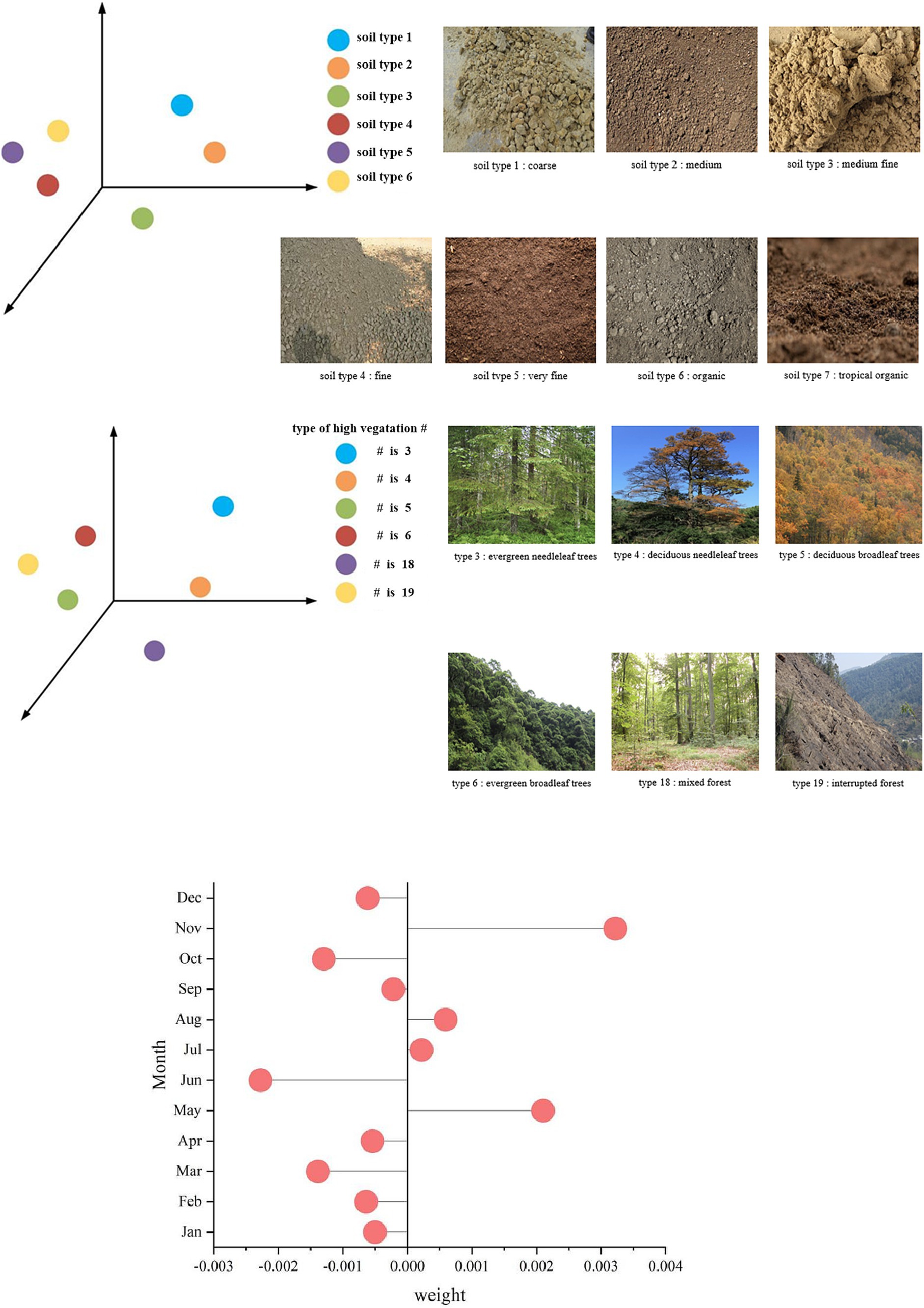
Figure 7. The spatial and temporal analysis of ISDNM retrievals. ST features for different soil types and type of high vegetation in China, mapped to 3D coordinates using UMAP. Monthly ISDNM determined weights indicating the contributions of ST in each month.
High vegetation type is another crucial factor in determining ST in any region (Owen et al., 1998). Figure 7 illustrates that the cosine distances for high vegetation types 5 (deciduous broadleaf trees) and 6 (evergreen broadleaf trees) are notably closer than those of other vegetation types. This is attributed to both these tree types being broadleaf varieties with overlapping distributions in China (Zheng-Yu et al., 2003). Furthermore, soils with denser vegetation covers retain moisture better than their sparser counterparts. This higher vegetation cover contributes to a slower decline in ST, as water possesses a greater heat capacity than soil. Higher soil moisture levels also equate to reduced fluctuations in ST. This is evident from Figures 2, 4, which indicate superior model results in southern China. One potential reason for this is the relatively stable atmospheric temperature in the south, as denoted by its reduced standard deviation, leading to more predictable changes in ST. This observation aligns with the findings of Cheng et al. (2008).
Lastly, from a temporal perspective, as observed in Figure 7, ST weights in May and November are notably higher than in other months. This suggests that these months play a pivotal role in our model’s ST prediction capabilities. An intriguing aspect is that May and November serve as inflection points in annual cycles (Huizhi et al., 2009; Tian et al., 2019). The trend in May’s ST has a cascading effect on June’s ST, resulting in May receiving greater weight and June less. A similar pattern is evident in November, given the more pronounced drop in ST observed in the preceding month of October (Huizhi et al., 2009; Tian et al., 2019).
4 Discussion
Several machine learning models, including MLP (Tabari et al., 2011, 2015), BPNN (Karandish and Shahnazari, 2016; Mehdizadeh et al., 2020), ELM (Sanikhani et al., 2018; Feng et al., 2019), GRNN (Feng et al., 2019), and RBNN (Kisi and Sanikhani, 2015; Feng et al., 2019), have been deployed for ST prediction, emphasizing their versatility and robustness. Nevertheless, deep learning methods are frequently labeled as “black box optimizers” due to their limited interpretative abilities.
In this context, the ISDNM model was introduced, which not only predicts ST but also incorporates spatio-temporal interpretative features, shedding light on the learning process using domain-specific knowledge. Specifically, ISDNM employs cosine distance to probe relationships between ST across varied categorical variables. Additionally, ISDNM is capable of determining linear regression coefficients, offering insights into the monthly contributions to the annual ST.
Addressing this perceived limitation, the ISDNM model emerged as a beacon, achieving great results both in predictive accuracy and model transparency. Beyond merely predicting ST, ISDNM seamlessly integrates spatio-temporal interpretative aspects, offering a more nuanced understanding of the underlying processes. Through its innovative use of cosine distance, the model provides an analytical lens to examine the relationships of ST across different categorical parameters. Moreover, its ability to determine linear regression coefficients paints a clear picture of monthly contributions to annual ST dynamics.
While our findings clearly demonstrated the superiority of the ISDNM over traditional models like CNN, LSTM, and ConvLSTM, it’s imperative to set these results against the backdrop of previous studies for a holistic perspective. Previous research primarily focused on achieving optimal prediction results, often sidelining the importance of interpretability. In contrast, the ISDNM not only showcases enhanced predictive capabilities but also champions the cause of interpretability, a feature often sought but rarely achieved in deep learning models. This dual capacity of the ISDNM model positions it favorably against its predecessors and contemporaries.
However, as with any scientific endeavor, it’s crucial to evaluate the practicality of this work. A region-specific assessment of the ISDNM’s efficacy highlighted areas in northeastern and northwestern China that require further attention, as evidenced by the pronounced RMSE values and diminished R2 scores depicted in Figure 2. Such regional disparities necessitate a deeper dive, and seasonal analyses provided further context. Figure 4’s depiction of ISDNM’s season-centric performance underscores the challenges faced during summer and winter, characterized by elevated RMSE and reduced R2 metrics.
The juxtaposition of the ISDNM model against previous studies underscores its unique position in the landscape of ST prediction. While it resonates with the accuracy that deep learning models are renowned for, it also paves the way for a new era where model transparency is not sacrificed. The debates around the practicality of such models will undoubtedly continue, but the ISDNM model has set a benchmark, indicating the direction future research might take in this domain.
5 Conclusion
ST stands as a critical element within the Essential Climate Variables as identified by GCOS, playing an instrumental role in numerous ecosystem processes and dynamics. Although deep learning methodologies have demonstrated significant potential in ST prediction, there remain reservations about their “black box” characteristics and limited physical interpretability. Moreover, accurately capturing the intricate spatio-temporal nuances of ST continues to pose challenges. To address these challenges above, the ISDNM model was introduced for ST prediction, utilizing ERA5 data. Trained on ERA5 data from 2015–2018 in China, with 2019 as the validation set and 2020 as the test set, ISDNM is structured in two distinct segments: the predictive and the interpretable components. While the predictive component is primarily engineered for feature extraction, the interpretable component elucidates both spatial and temporal correlations of ST.
Comprehensive assessments of ERA5-based ST via the ISDNM model highlight its remarkable advantage over conventional deep learning techniques. By integrating the CNN-encoder-decoder with the LSTM-encoder-decoder architectures, ISDNM attained the best performance. The standout attribute of ISDNM lies in its ability to provide insights, facilitating the extraction of spatio-temporal characteristics of ST. This design effectively delineates the associations between diverse categorical variables in connection with ST and discerns the temporal shifts in ST.
However, like all models, the ISDNM has its limitations. While it exhibits robust predictive and interpretative capabilities, it primarily relies on ERA5 data, which may introduce biases or errors inherent to this specific dataset. The model’s performance in regions outside China, or under different climatic conditions, remains to be ascertained. Additionally, its dependence on CNN-encoder-decoder and LSTM-encoder-decoder architectures might limit its adaptability to newer or alternative deep learning techniques.
Looking to the future, there is potential to refine the ISDNM model by incorporating more diverse datasets to enhance its generalizability. Furthermore, exploring the integration of newer deep learning techniques or alternative architectures could elevate its predictive and interpretative capacities. The pronounced impact of months like May and November on yearly ST predictions also suggests avenues for targeted, seasonal investigations. Future studies will delve deeper into these aspects, further exploring the complex dynamics governing the ISDNM model in the realm of ST.
Simultaneously, the quality of the dataset will be enhanced by incorporating station data and diverse satellite information, aiming to achieve even more competitive outcomes.
Author contributions
XL: Conceptualization, Writing – original draft. YZ: Software, Writing – review & editing. QL: Resources, Writing – original draft. HZ: Validation, Writing – review & editing. JZ: Resources, Writing – original draft. CZ: Software, Writing – review & editing.
Funding
The author(s) declare financial support was received for the research, authorship, and/or publication of this article. This study was partially supported by the National Natural Science Foundation of China, grant numbers 42105144, 4227515, 41975122, 42205149, and U1811464, the Jilin Provincial Science and Technology Development Plan Project under grant 20220203184SF and the Jilin Provincial Department of Education Science and Technology Research Project under grants JJKH20220840KJ and JJKH20230919KJ.
Conflict of interest
The authors declare that the research was conducted in the absence of any commercial or financial relationships that could be construed as a potential conflict of interest.
Publisher’s note
All claims expressed in this article are solely those of the authors and do not necessarily represent those of their affiliated organizations, or those of the publisher, the editors and the reviewers. Any product that may be evaluated in this article, or claim that may be made by its manufacturer, is not guaranteed or endorsed by the publisher.
References
Beck, H. E., Zimmermann, N. E., Mcvicar, T. R., Vergopolan, N., Berg, A., and Wood, E. F. (2018). Present and future Kppen-Geiger climate classification maps at 1-km resolution. Sci. Data 5:180214. doi: 10.1038/sdata.2018.214
Bodić, M, Vuković, P, Rajs, V, Vasiljević-Toskić, Marko, and Bajić, Jovan (2018). Station for soil humidity, temperature and air humidity measurement with SMS forwarding of measured data. Proceedings of the 2018 41st international spring seminar on electronics technology (ISSE). Zlatibor, Serbia: IEEE.
Cheng, H., Wang, G., Hu, H., and Wang, Y. (2008). The variation of soil temperature and water content of seasonal frozen soil with different vegetation coverage in the headwater region of the Yellow River, China. Environ. Geol. 54, 1755–1762. doi: 10.1007/s00254-007-0953-x
Cho, K., Van Merriënboer, B., Bahdanau, D., and Bengio, Y. (2014). On the properties of neural machine translation: encoder-decoder approaches. ar Xiv [Preprint arXiv]. doi: 10.48550/arXiv.1409.1259
Cobaner, M., Citakoglu, H., Kisi, O., and Haktanir, T. (2014). Estimation of mean monthly air temperatures in Turkey. Comput. Electron. Agric. 109, 71–79. doi: 10.1016/j.compag.2014.09.007
Cornu, J. Y., Denaix, L., Lacoste, J., Sappin-Didier, V., Nguyen, C., and Schneider, A. (2016). Impact of temperature on the dynamics of organic matter and on the soil-to-plant transfer of Cd, Zn and Pb in a contaminated agricultural soil. Environ. Sci. Pollut. Res. 23, 2997–3007. doi: 10.1007/s11356-015-5432-4
Feng, Y., Cui, N., Hao, W., Gao, L., and Gong, D. (2019). Estimation of soil temperature from meteorological data using different machine learning models. Geoderma 338, 67–77. doi: 10.1016/j.geoderma.2018.11.044
GCOS (2016). The global observing system for climate: implementation needs. Global Climate Observation System.
Guo, C., and Berkhahn, F. (2016). Entity embeddings of categorical variables. arXiv [Preprint arXiv]. doi: 10.48550/arXiv.1604.06737
Hao, H., Yu, F., and Li, Q. (2020). Soil temperature prediction using convolutional neural network based on ensemble empirical mode decomposition. IEEE Access 9, 4084–4096. doi: 10.1109/ACCESS.2020.3048028
Henderson-Sellers, A., Yang, Z. L., and Dickinson, R. E. (1993). The project for intercomparison of land-surface parameterization schemes. Bull. Am. Meteorol. Soc. 74, 1335–1349. doi: 10.1175/1520-0477(1993)074<1335:TPFIOL>2.0.CO;2
Hochreiter, S., and Schmidhuber, J. (1997). Long short-term memory. Neural Comput. 9, 1735–1780. doi: 10.1162/neco.1997.9.8.1735
Huizhi, Z., Shi Xuezheng, Y., Dongsheng, W. H., Yongcun, Z., Weixia, S., and Baorong, H. (2009). Seasonal and regional variations of soil temperature in China. Acta Pedol. Sin. 46, 227–234. doi: 10.11766/200709280206
Hulugalle, N. R., Entwistle, P. C., Scott, F., and Kahl, J. (2001). Rotation crops for irrigated cotton in a medium-fine, self-mulching, grey Vertosol. Soil Res. 39:317. doi: 10.1071/SR00035
Hyndman, R. J., and Koehler, A. B. (2006). Another look at measures of forecast accuracy. Int. J. Forecast. 22, 679–688. doi: 10.1016/j.ijforecast.2006.03.001
Kalakuntla, R., Wille, T., Provost, R. L., Letort, S., Reite, G., Müller, S., et al. (2013). Analysis of the linearised observation operator in a land surface data assimilation scheme for numerical weather prediction. Toxicol. Lett. 216, 200–205. doi: 10.1016/j.toxlet.2012.11.020
Karandish, F., and Shahnazari, A. (2016). Soil temperature and maize nitrogen uptake improvement under partial root-zone drying irrigation. Pedosphere 26, 872–886. doi: 10.1016/S1002-0160(15)60092-3
Kim, Y., Still, C. J., Hanson, C. V., Kwon, H., Greer, B. T., and Law, B. E. (2016). Canopy skin temperature variations in relation to climate, soil temperature, and carbon flux at a ponderosa pine forest in Central Oregon. Agric. For. Meteorol. 226-227, 161–173. doi: 10.1016/j.agrformet.2016.06.001
Kisi, O., Kim, S., and Shiri, J. (2013). Estimation of dew point temperature using neuro-fuzzy and neural network techniques. Theor. Appl. Climatol. 114, 365–373. doi: 10.1007/s00704-013-0845-9
Kisi, O., and Sanikhani, H. (2015). Modelling long-term monthly temperatures by several data-driven methods using geographical inputs. Int. J. Climatol. 35, 3834–3846. doi: 10.1002/joc.4249
LeCun, Y., Boser, B., Denker, J. S., Henderson, D., Howard, R. E., Hubbard, W., et al. (1989). Backpropagation applied to handwritten zip code recognition. Neural Comput. 1, 541–551. doi: 10.1162/neco.1989.1.4.541
Li, Q., Hao, H., Zhao, Y., Geng, Q., Liu, G., Zhang, Y., et al. (2020). GANs-LSTM model for soil temperature estimation from meteorological: a new approach. IEEE Access. 8, 59427–59443. doi: 10.1109/ACCESS.2020.2982996
Li, Q., Li, Z., Shangguan, W., Wang, X., Li, L., and Yu, F. (2022b). Improving soil moisture prediction using a novel encoder-decoder model with residual learning. Comput. Electron. Agric. 195:106816. doi: 10.1016/j.compag.2022.106816
Li, L., Shangguan, W., Deng, Y., Mao, J., and Dai, Y. (2020). A causal-inference model based on random forest to identify the effect of soil moisture on precipitation. J. Hydrometeorol. 21, 1115–1131. doi: 10.1175/JHM-D-19-0209.1
Li, Q., Wang, Z., Shangguan, W., Li, L., Yao, Y., and Yu, F. (2021). Improved daily SMAP satellite soil moisture prediction over China using deep learning model with transfer learning. J. Hydrol. 600:126698. doi: 10.1016/j.jhydrol.2021.126698
Li, Q., Zhu, Y., Shangguan, W., Wang, X., Li, L., and Yu, F. (2022a). An attention-aware LSTM model for soil moisture and soil temperature prediction. Geoderma 409:115651. doi: 10.1016/j.geoderma.2021.115651
McInnes, L., Healy, J., and Melville, J. (2018). UMAP: uniform manifold approximation and projection for dimension reduction. arXiv [Preprint arXiv]. doi: 10.48550/arXiv.1802.03426
Mehdizadeh, S., Fathian, F., Safari, M. J. S., and Khosravi, A. (2020). Developing novel hybrid models for estimation of daily soil temperature at various depths. Soil Tillage Res. 197:104513. doi: 10.1016/j.still.2019.104513
Mohammadi, K., Shamshirband, S., Kamsin, A., Lai, P. C., and Mansor, Z. (2016). Identifying the most significant input parameters for predicting global solar radiation using an ANFIS selection procedure. Renew. Sust. Energ. Rev. 63, 423–434. doi: 10.1016/j.rser.2016.05.065
Owen, T. W., Carlson, T. N., and Gillies, R. R. (1998). An assessment of satellite remotely-sensed land cover parameters in quantitatively describing the climatic effect of urbanization. Int. J. Remote Sens. 19, 1663–1681. doi: 10.1080/014311698215171
Ran, C., Bai, X., Tan, Q., Luo, G., Cao, Y., Wu, L., et al. (2023). Threat of soil formation rate to health of karst ecosystem. Sci. Total Environ. 887:163911. doi: 10.1016/j.scitotenv.2023.163911
Reichstein, M., Camps-Valls, G., Stevens, B., Jung, M., Denzler, J., Carvalhais, N., et al. (2019). Deep learning and process understanding for data-driven earth system science. Nature 566, 195–204. doi: 10.1038/s41586-019-0912-1
Ronda, R. J., and Bosveld, F. C. (2009). Deriving the surface soil heat flux from observed soil temperature and soil heat flux profiles using a variational data assimilation approach. J. Appl. Meteorol. Climatol. 48, 644–656. doi: 10.1175/2008JAMC1930.1
Sanikhani, H., Deo, R. C., Yaseen, Z. M., Eray, O., and Kisi, O. (2018). Non-tuned data intelligent model for soil temperature estimation: a new approach. Geoderma 330, 52–64. doi: 10.1016/j.geoderma.2018.05.030
Shang, M., and Luo, J. (2021). The tapio decoupling principle and key strategies for changing factors of Chinese urban carbon footprint based on cloud computing. Int. J. Environ. Res. Public Health 18:2101. doi: 10.3390/ijerph18042101
Tabari, H., Hosseinzadeh Talaee, P., and Willems, P. (2015). Short-term forecasting of soil temperature using artificial neural network. Meteorol. Appl. 22, 576–585. doi: 10.1002/met.1489
Tabari, H., Sabziparvar, A. A., and Ahmadi, M. (2011). Comparison of artificial neural network and multivariate linear regression methods for estimation of daily soil temperature in an arid region. Meteorog. Atmos. Phys. 110, 135–142. doi: 10.1007/s00703-010-0110-z
Tian, H., Huang, N., Niu, Z., Qin, Y., Pei, J., and Wang, J. (2019). Mapping winter crops in China with multi-source satellite imagery and phenology-based algorithm. Remote Sens. 11:820. doi: 10.3390/rs11070820
Valipour, M. (2015). Importance of solar radiation, temperature, relative humidity, and wind speed for calculation of reference evapotranspiration. Arch. Agron. Soil Sci. 61:239. doi: 10.1080/03650340.2014.925107
Wei, X., Bai, X., Wen, X., Liu, L., Xiong, J., and Yang, C. (2023). A large and overlooked cd source in karst areas: the migration and origin of Cd during soil formation and erosion. Sci. Total Environ. 895:165126. doi: 10.1016/j.scitotenv.2023.165126
Willmott, C. J., and Matsuura, K. (2005). Advantages of the mean absolute error (MAE) over the root mean square error (RMSE) in assessing average model performance. Clim. Res. 30, 79–82. doi: 10.3354/cr030079
Xu, J., Lan, W., Ren, C., Zhou, X., Wang, S., and Yuan, J. (2021). Modeling of coupled transfer of water, heat and solute in saline loess considering sodium sulfate crystallization. Cold Reg. Sci. Technol. 189:103335. doi: 10.1016/j.coldregions.2021.103335
Yan, X., Liang, C., Jiang, Y., Luo, N., Zang, Z., and Li, Z. (2020). A deep learning approach to improve the retrieval of temperature and humidity profiles from a ground-based microwave radiometer. IEEE Trans. Geosci. Remote Sens. 58, 8427–8437. doi: 10.1109/TGRS.2020.2987896
Yan, Y., Yan, R., Chen, J., Xin, X., Eldridge, D. J., Shao, C., et al. (2018). Grazing modulates soil temperature and moisture in a Eurasian steppe. Agric. For. Meteorol. 262, 157–165. doi: 10.1016/j.agrformet.2018.07.011
Yang, J., Busen, H., Scherb, H., Hürkamp, K., Guo, Q., and Tschiersch, J. (2019). Modeling of radon exhalation from soil influenced by environmental parameters. Sci. Total Environ. 656, 1304–1311. doi: 10.1016/j.scitotenv.2018.11.464
Yin, L., Wang, L., Li, T., Lu, S., Yin, Z., Liu, X., et al. (2023). U-Net-STN: a novel end-to-end lake boundary prediction model. Land 12:1602. doi: 10.3390/land12081602
Yuan, J., Li, Y., Shan, Y., Tong, H., and Zhao, J. (2023). Effect of magnesium ions on the mechanical properties of soil reinforced by microbially induced carbonate precipitation. J. Mater. Civ. Eng. 35:04023413. doi: 10.1061/JMCEE7.MTENG-15080
Zhang, G., Zhao, Z., Yin, X. A., and Zhu, Y. (2021). Impacts of biochars on bacterial community shifts and biodegradation of antibiotics in an agricultural soil during short-term incubation. Sci. Total Environ. 771:144751. doi: 10.1016/j.scitotenv.2020.144751
Zhao, L., Yang, K., Qin, J., Chen, Y., Tang, W., Montzka, C., et al. (2013). Spatiotemporal analysis of soil moisture observations within a Tibetan mesoscale area and its implication to regional soil moisture measurements. J. Hydrol. 482, 92–104. doi: 10.1016/j.jhydrol.2012.12.033
Zheng, D., Hunt, E. R., and Running, S. W. (1993). A daily soil temperature model based on air temperature and precipitation for continental applications. J. Appl. Entomol. 123, 183–191. doi: 10.3354/cr002183
Keywords: soil temperature, deep learning, interpretable model, machine learning (ML), LSTM (long short term memory networks)
Citation: Li X, Zhu Y, Li Q, Zhao H, Zhu J and Zhang C (2023) Interpretable spatio-temporal modeling for soil temperature prediction. Front. For. Glob. Change. 6:1295731. doi: 10.3389/ffgc.2023.1295731
Edited by:
Gabriele Broll, Osnabrück University, GermanyReviewed by:
Ahmed Elbeltagi, Mansoura University, EgyptAnurag Malik, Punjab Agricultural University, India
Copyright © 2023 Li, Zhu, Li, Zhao, Zhu and Zhang. This is an open-access article distributed under the terms of the Creative Commons Attribution License (CC BY). The use, distribution or reproduction in other forums is permitted, provided the original author(s) and the copyright owner(s) are credited and that the original publication in this journal is cited, in accordance with accepted academic practice. No use, distribution or reproduction is permitted which does not comply with these terms.
*Correspondence: Qingliang Li, bGlxaW5nbGlhbmdAY2NzZnUuZWR1LmNu