 Jan Schick1,2*†
 Matthias Albert
 Matthias Schmidt
95% of researchers rate our articles as excellent or good
Learn more about the work of our research integrity team to safeguard the quality of each article we publish.
Find out more
ORIGINAL RESEARCH article
Front. For. Glob. Change , 24 August 2023
Sec. Forest Growth
Volume 6 - 2023 | https://doi.org/10.3389/ffgc.2023.1201636
This article is part of the Research Topic Approaches for Modelling the Effects of Climate Change on the Productivity and Growth in Managed Forest Resources for Timber Production View all 4 articles
Introduction: We developed a new approach for site index curve models that combines longitudinal height development patterns derived from state-space data with the broad environmental conditions covered by space-for-time data.
Methods: For this, we gathered dendrometry from both inventories and research plots. Concerning environmental variables, we included soil mapping data as well as atmospheric data, i.e., precipitation, temperature, and nitrogen deposition. The atmospheric data was included as a weighted mean over the stand life of the sums for the dynamically determined vegetation period or as yearly sums in the case of nitrogen deposition, respectively. As a weight, the values of a height increment function were used. Then, we derived the basic shape of a height development curve from research plot data and transferred said shape to a site index curve model.
Results: The model represents a substantial advancement of a previous version and was fitted as a generalized additive model (GAM). All effects were of relevant size and showed biologically feasible patterns.
Discussion: Though the model is biased for young ages, we could predict site index curves that, under constant environmental conditions, closely follow yield table curves and thus accurately depict stand height development. Moreover, the model does not require initial dendrometry, which broadens its applicability. Thus, the model represents a useful tool for forest management and planning under climate change.
Nowadays, forest ecosystems and forest enterprises are substantially affected by rapidly changing environmental conditions (Lindner et al., 2014). In many parts of the world and especially in large areas in Central Europe, gradual processes have transformed site quality negatively through exploitation, or positively through, for example, site-enhancing species by reforestation in the last centuries (Koch and Skovsgaard, 1999). However, massive nitrogen and sulfur depositions beginning in the 1950s (Schöpp et al., 2003) and the rapidly changing climate affect the primary growing conditions of forests well below a classical rotation period (Boisvenue and Running, 2006; Aertsen et al., 2014; Kohnle et al., 2014; Pretzsch et al., 2014). Concerning the prediction of prospective forest growth and yield, the long-time assumed paradigm in forest management to assume constant site conditions has to be revised at least for a stand's lifespan (Pretzsch, 1992; Skovsgaard and Vanclay, 2008; Smith et al., 2015). Consequently, the previously applied static biological laws of growth and yield need to be adapted to account for aggravating transitions in site conditions. This calls for new forest management tools to brace for the challenges of climate change. The development of site-productivity models sensitive to changing environmental conditions is a prerequisite for such new forest management tools.
In the recent past, new approaches in statistical forest growth modeling account for dynamic site conditions either as space-for-time substitutions (SFTS, see Pickett, 1989) or applying the state-space approach (SSA, see García, 1994; Auger-Méthé et al., 2021). Typically, growth models based on SFTS principle use spatially wide spread data from National Forest Inventories or other inventory sources in order to acquire a broad range of environmental conditions along gradients (e.g., Monserud et al., 2006; Albert and Schmidt, 2010; Nothdurft et al., 2012; Antón-Fernández et al., 2016). Thus, inventory data shows a large between-plot variance, which allows to cover the amplitude of the relevant environmental factors to model forest growth (Álvarez González et al., 2014). However, ecological data collected at one point in time or repeatedly over a short period of time is not suited to reveal the effects of changing environmental conditions on forest growth. SSA, on the other hand, relies on longitudinal growth data, i.e., long-term time series, to capture the growth response to changing conditions over time (e.g., Zhang and Borders, 2001; Nord-Larsen and Johannsen, 2007; Yue et al., 2016). Thus, SSA is suited to account for stand-by-environment interaction (Yue et al., 2023). However, long time-series are mostly available for experimental growth and yield trials only, which are limited in number and thus do not cover all combinations of the relevant environmental factors (Nagel et al., 2012).
In the context of climate change impact studies, SFTS is currently under debate. Damgaard (2019) argues that as ecosystems are influenced by a multitude of different processes simultaneously which operate on different time-scales a simple substitution of growth processes observed over an environmental gradient for growth predictions in time could be erroneous. Klesse et al. (2020) also refute SFTS as they observe radial growth response to temperature variation of Douglas-fir being opposite in sign regarding spatial and temporal variation. Thus, spatial variation in productivity cannot unrestrictedly be used to project changes in productivity caused by temporal factors as, for example, climate change. Yue et al. (2023) advocate SSA over SFTS as their study on Norway spruce stands shows significant effects of stand-by-environment interaction on site index response. Also, the concern about potential confounding in the SFTS should be considered, since gradient studies often lack a randomization and interspersion of treatments in the meaning of manipulated experiments (Hurlbert, 1984).
On the other hand, in the context of area-wide applicability of a growth model, SSA often lacks data for generalization (Adler et al., 2012; Nagel et al., 2012; Damgaard, 2019; Pretzsch et al., 2019). While long-term forest experiment sites provide an ideal database for causal analysis, for example the effect of species mixture on growth, tools for practical forest management need to be applicable at any site, i.e., over a wide area. Thus, unambiguous recommendations to unrestrictedly replace SFTS approaches with SSA based on long-term longitudinal data cannot be given yet (e.g., Albrecht et al., 2017; Waldy et al., 2021).
In our analysis, we therefore followed the advice by Damgaard (2019) and combined SFTS with SSA data, i.e., long time-series data from a relatively small number of research plots and inventory data with only a few repeated measurements but covering a wide spatial gradient. The importance of the scale level concerning the validity of empirical site index models was already emphasized by Aertsen et al. (2012). Moreover, the long time-series of the research plots not only contain longitudinal characteristics, but also measurements under past environmental conditions, most importantly with lower nitrogen deposition, such that the corresponding causal relationships can be identified more clearly. Hence, we could derive longitudinal patterns of stand height development as well as causal relationships of environmental influences in hierarchical, statistical models, whose results are applicable to a broad range of site conditions (cp. Nagel et al., 2012; Damgaard, 2019).
It is our goal in the presented research to introduce a practical model to project stand height development under a changing climate for forest management and planning. We derived a new modeling approach for predicting the development of stand height over age, i.e., a site index curve model (SICM), taking European beech (Fagus sylvatica L.) as an example. As central features for such a useful tool we determine (1) sensitivity regarding essential environmental influences, with relevant and plausible effects, such that (2) estimations with spatially and longitudinally sound patterns can be achieved and differences between sites are correctly depicted. This generalization of the results implies, that we require (3) data, which is available on a broad environmental scale as well as long time series data to derive the longitudinal characterstics.
As a starting point in model development, we refer to the previous climate and site sensitive site index curve model by Schmidt (2020) (SICMprev), which used SFTS data to predict stand height development under varying environmental conditions. In the following, we focus on European beech as an example. The original data is described in Section 2.1, Section 2.2 deals with further processing of said data.
The data used for model development can be separated into dendrometric data (height, diameter, age and species) and environmental data (temperature, precipitation, nitrogen deposition, soil categories and, as a proxy, coordinates).
The majority of the data was obtained from forest inventories. Firstly, the national forest inventories of Germany (NFI) from 1987, 2002, and 2012, respectively (Federal Ministry of Food and Agriculture, 2016). Here, data was gathered from a systematic cluster sample for all of Germany. A systematic grid was placed over Germany, with grid length being either 4 km × 4 km, 2.83 km × 2.83 km, or 2 km × 2 km, depending on the federal state. At each knot of the grid, four plots were placed at the corners of a 150 m × 150 m square. Plots outside of the forest were excluded. At each plot, angle-count sampling was performed, only including trees with a diameter at breast height (DBH), i.e., the diameter at 1.3 m, >7 cm (10 cm for the first NFI). All DBHs of the respective trees were measured. During the first NFI, all corresponding heights were measured as well. Note, that due to the separation of Germany until 1990, the “first” NFI was either 1987 or 2002, depending on the federal state. The following NFIs only took height measurements representative for species and layer (Federal Ministry of Food and Agriculture, 2016).
Furthermore, we included data from an inventory in 2017, which was used to assess carbon storage in German forests (CFI). The design is equal to the NFI, except that the base grid was expanded to 8 km × 8 km. All measurements were performed on NFI plots. We used the CFI data of the states Hessia, Lower Saxony, Schleswig-Holstein and Saxony-Anhalt.
We also included enterprise inventories (EFI) of the state owned forests of the four aforementioned states. Here, measurements were taken on fixed concentric sample plots with two radii, 6 m for trees with 7 cm ≤ DBH < 30 cm and 13 m for trees with DBH ≥ 30 cm. All DBHs were recorded as well as heights representative for species and layer. The plots are placed on fixed grids, whose width varies between states and forest districts.
Apart from the inventory data, we included data from long term research plots from the Northwest German Forest Research Institute (NW-FVA). The plots are located mainly in the northwest of Germany, i.e., the jurisdiction of the NW-FVA, and are of varying size and research aim. Measurements were available from the year 1890 to 2021, depending on the plot, and were taken on average every five years. For each measurement occasion, all DBHs were measured as well as a high number of representative heights.
Lastly, we conduct a special measurement campaign within the jurisdiction of the NW-FVA, to acquire data on forests, whose soil and climatic properties were underrepresented in our dataset. At each location, a sample was selected via angle-count and the corresponding DBHs and heights have been measured. As of now, measurements have been taken in the inner German dry zone in Saxony-Anhalt.
Generally speaking, the inventory data is characterized by great spatial variation combined with few repeated measurements. That is, we have 58,022 individual plots with an average of 1.5 measurement occasions taken, on average, every 6.0 years per plot. The inverse holds true for the research plots, where the average number of measurement occasions per plot is 6.8, taken on 258 individual plots every 4.7 years. For a distribution of the data across Germany (see Figure 1).
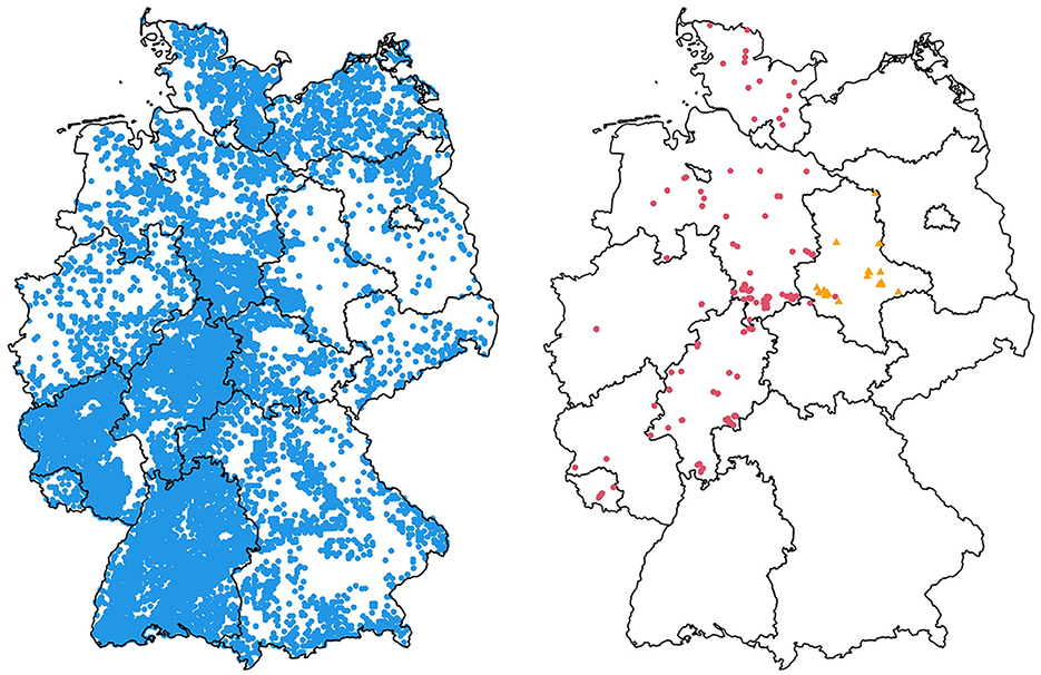
Figure 1. Locations of measurement plots in Germany, separated by source. Inventory data is shown on the left (blue), research plot data is on the right (red circles), as are the specially selected forests with rare site conditions from the inner German dry zone in Saxony-Anhalt (orange triangles).
For the final dataset, a number of filtering criteria were applied. We only considered plots with beech as leading species in the upper story. The trees measured in the inventories already had been classified into upper and lower story based on expert assessment in the field. However, for the research plot data no consistent classification was available. Hence, we used an algorithm to separate the stratums. The methodology can be found in ch. 2.2.1. Furthermore, the age span of the plots was not allowed to be >10% of the mean age. As we model a height-age relationship on the stand level, a wide range of ages within a stand would distort the results. Trees with an age larger than 250 years were also excluded to avoid an unbalanced design at the extremes of the age distribution, since stands usually only get to such a high age on poor sites. Outlier selection was performed both considering the height-age as well as the height-diameter relationships within the plots. For this, we used quantiles and visual checks to determine and exclude values deemed to be unrealistic.
After applying all filtering criteria, the number of plot measurement occasions was 30,198 for the NFIs, 1,090 for the CFI, 57,914 for the EFIs, 1,763 for the research plots and, as of now, 26 for the measurement campaign. Hence, the final dataset contains 90,991 plot measurement occasions.
Climatic conditions for tree growth were depicted by annual temperature and precipitation sums for the respective vegetation period. For this, raw climate data were retrieved as daily mean temperature and daily precipitation sums for the years 1900 to 2019 from the official weather stations of the German Meteorological Service (DWD). These values were then summed for the vegetation period, which was determined dynamically, with start and end date calculated according to Menzel (1997) and Nuske (2017). This dynamic approach allowed, that annual differences in the vegetation period could be accounted for. The point data, i.e., the sums, for the locations of the respecitve weather stations were then regionalized to a 50 m × 50 m grid covering Germany. For this, we utilized a generalized additive model (GAM) with two effects: A spatial smoother to interpolate between the weather stations, and another spline to account for the effect of elevation.
The deposition fluxes of nitrogen were modeled from the mapped atmospheric deposition data for Germany that were provided by the Federal Environment Agency (UBA) (Schaap et al., 2018). For each grid cell (1 km × 1 km), land cover type specific deposition rates are available, including coniferous forest, deciduous forest, and mixed forest. Thus, deposition rates at the forest growth monitoring sites were extracted from the modeled results based on site coordinates and tree species. These data only cover the period from 2000 to 2015. To obtain the nitrogen deposition time series from 1800 to 2022 for each forest growth monitoring site, temporal reconstruction methods were adapted. Following the approach described by Ahrends et al. (2022) for sulfur, a standard scaling function was created. This function was based on the trend of nitrogen deposition for Europe described by Engardt et al. (2017) (from 1900 to 2050) and by Alveteg et al. (1998) (from 1800 to 1900). Due to the high uncertainties in the quantification of nitrogen inputs (Ahrends et al., 2020), the trends from two different chemical transport models (MATCH and the EMEP MSC-W model, cp. Engardt et al., 2017) were averaged.
We also used data from forest soil mapping to include categories characterizing capacity of available water as well as possible influences of groundwater and waterlogging (water budget category, WBC) as well as nutrient availibility of the soil (nutrient budget category, NBC). WBC and NBC are coded in three different schemes: Lower Saxony (NFP, 2007, 2009), Hessia (HessenForst, 2017) and a synopsis developed during a project assessing forest growth and carbon storage under climate change (WP-KS-KW, see Benning et al., 2020). The latter being intended as a unifying synopsis for Germany. However, using only said synopsis would lead to information loss (see ch. 4.1). Each scheme contains NBC ranging from poor to rich soils and WBC for different water conditions, with special categories for hydromorphic and groundwater influenced soils. The scheme of Lower Saxony also differentiates between uplands and lowlands. We also categorized data from the unifying synopsis into uplands and lowlands, according to the large scale forestry landscapes (Thünen-Institut, 2011). Based on the same reference, Hessia only consists of uplands. In total, a complete set of WBC and NBC was available for 89% of the measurements. The remaining measurements have been set to an unknown category, separated into uplands and lowlands. This was done to still include the remaining covariates, e.g., temperature and precipitation, into the model. Otherwise said information could not have been accounted for in the model effects.
Before building the model, the data had to be processed further, i.e., computing the mean quadratic diameter tree (Dq) and the corresponding height (Hq) for the upper story of each plot. Moreover, the atmospheric data is further modified, i.e., a height increment function is used to compute a weighted mean and the temperature is corrected for aspect and slope.
All modeling was done with R version 4.1.1 (R Core Team, 2021). We used the packages gamm4 version 0.2-6 (Wood and Scheipl, 2020) for generalized mixed model approaches (see ch. 2.2.2), and mgcv version 1.8-41 (Wood, 2017) for fitting GAMs (see ch. 2.2.1, 2.2.3, 2.2.4).
Since we model the height development of the main stand, we only considered trees of the upper story. In the inventory data, the trees of the upper story were already labeled. For the research plots, the stratums of the canopy layer were not fully classified. Staupendahl (2022) developed an automated stratum separator, which classifies a stand into upper story and, if feasible, lower story. This is done by examining height and diameter of each measurement occasion. If groups of trees with different height-diameter characteristics, i.e., upper and lower story, can be identified, a bimodal and bivariate Gaussian distribution is fitted. Depending on the densitiy of the distribution, each tree is classified as upper or lower story. If no groups can be identified, the whole stand is classified as upper story (Staupendahl, 2022). We then applied further adaptions to the stratum separator, to ensure, that the classification is consistent over time. This was done by modeling the mean value of the DBH, at which the stratums were separated, over stand age, and using the resulting value to classify the trees into upper and lower story based on their DBH. However, this was only used after the first occurence of a lower story within a stand, according to the aforementioned algorithm. Further rule-based corrections were applied to ensure plausibility of the results. That is, tree height measurements, where present, were used, such that the tallest trees were always classified as upper story and the smallest ones as lower story.
As a measure of stand growth and site index, we chose the Hq. It is defined as the height corresponding Dq, which, for stand k at time t, is calculated as
with n being the number of trees measured on this measurement occasion and dbhkti being the dbh of the ith tree of stand k at time t. To obtain a height, we then fitted a modified Korf function, originally developed by Lappi (1997) and based on Korf (1939), to each plot. Said function will be described in more detail in ch. 2.2.4. We used a generalized linear mixed model (GLMM) with a Gamma distribution and log-link, as well as random intercept on the level of the measurement occasion as in Equation 2a for the inventories. For the research plots, a higher number of measurement occasions with a higher number of individual tree measurements, respectively, were available. Thus, we could nest the random effect for measurement occasion within the plot effect and, moreover, include a random slope (Equation 2b).
or:
with:
and:
with α0 and α1 being the fixed effects, τ0kt being the random intercept for each measurement occasion used for the inventory data. For the research plot data, ρ0 and ρ1 are the fixed effects, ψ0k and ψ1k the random effects on the plot level, and ν0kt and ν1kt the random effects for measurement occasions. dbhkti represents the dbh of tree i in stand k at time t. The parameters ω, φ0, φ1, π0, and π1 are the standard deviations of the corresponding random effects. λdbh and cdbh are parameters and were set to the values determined by Schmidt (2010), i.e., 20 and to 2.2, respectively.
The measurement-occasion-specific height-diameter curves generated by said model were then used, to predict the height corresponding to the Dq of each measurement occasion, i.e., the Hq.
To include the atmospheric variables (temperature, precipitation, nitrogen deposition) into the model, they first had to be aggregated to a single value for each Hq.
In the SICMprev, Schmidt (2020) calculated an unweighted mean over stand life for all atmospheric variables. We replaced this by a mean weighted with a species specific height increment function to better account for stand growth dynamics. For this, the function developed by Sloboda (1971) was parameterized with the data from the NW-FVA research sites, depending on the age and the site index of a stand. For the final function, a Hq of 30.8 m at age 100 was chosen as site index, representing the mean site index of the research plots. The respective function can be seen in Figure 2. Finally, the weighted mean is given as
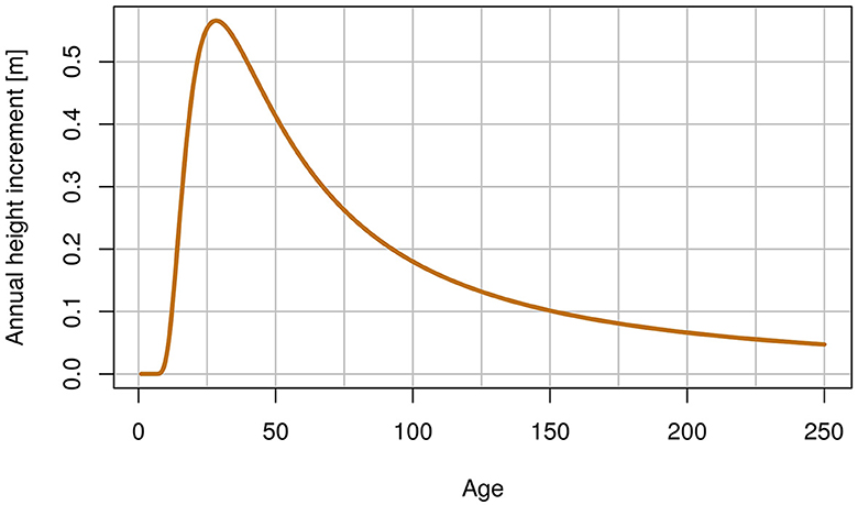
Figure 2. Height increment curves based on the formula of Sloboda (1971) for European beech with a Hq of 30.8 m at age 100 as a site index.
with agekt being the age of stand k at time t, ϕk(i) being the value of the respective atmospheric variable for stand k at age i and w(i) being the value of the growth function (see Figure 2) at age i.
To further account for the influences of topography, we additionally corrected the temperature for aspect and slope according to the water balance simulation model WaSiM (Schulla, 2021). The latter is originally used to correct daily temperatures based on physical laws. To apply the correction to our data, we acquired corrected, daily temperatures for the respective vegetation period. We then used a GAM as specified in Equation 4 to extract the correction mechanism. The final temperature correction induced by the model, depending on aspect and slope, can be seen in Figure 3.
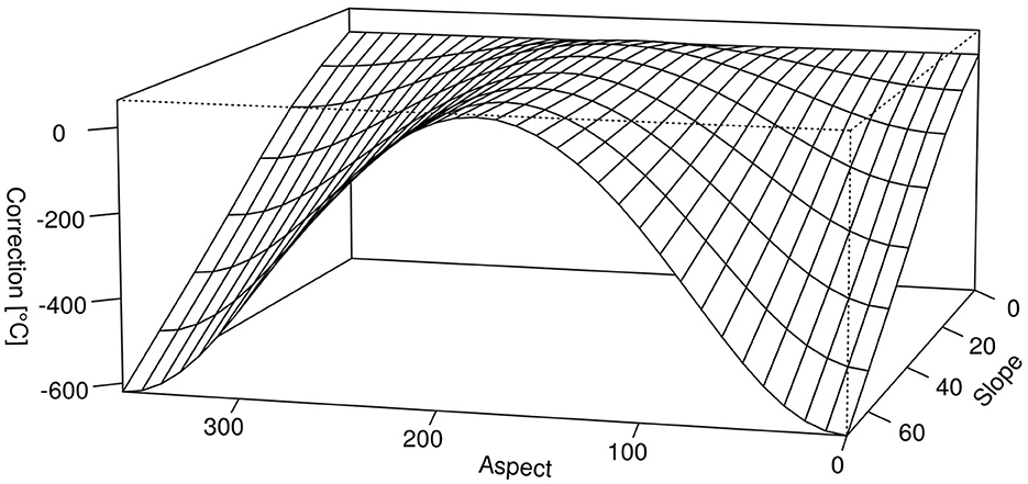
Figure 3. Correction for temperature sums during the vegetation period as a function of aspect and slope. Aspect is given in degrees with 0 being North, 180 being South. Slope is given in degrees with 0 being flat ground.
with:
Hereafter, the fully processed temperature, precipitation and nitrogen deposition will be called tempsum_veg, precsum_veg and Ndep, respectively. That is, a weighted mean over stand life of the corresponding covariate sum, i.e., the sum over the vegetation period for tempsum_veg and precsum_veg, and the yearly sum for Ndep. Moreover, tempsum_veg has been corrected for aspect and slope. Finally, we computed an aridity index by dividing precsum_veg by tempsum_veg, denoted aridity_veg.
This finalized the dataset, characteristics of which are displayed in Table 1. The data is shown separated by source to indicate the comparability of the different data sources. Moreover, the correlation between the variables within the final data is shown in Figure 4.
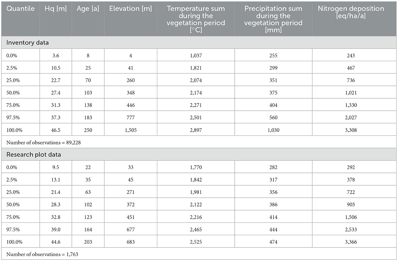
Table 1. Quantiles of covariates on plot measurement scale used for the development of site sensitive site index curves for beech.
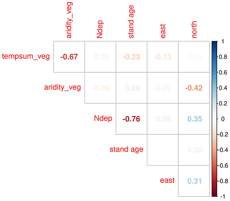
Figure 4. Upper triangle of the correlation matrix of the site data used for fitting the model.
The goal of the modeling process was to develop a climate- and site-sensitive SICM, which can predict the Hq of a beech stand at a given age for all of Germany. This required several steps, that is, (1) choosing a suitable height development function as a basis. Here, we chose a modification of the Korf function (Korf, 1939), originally derived by Lappi (1997) and further modified by Schmidt (2020). (2) Define the basic shape of the modified Korf function. (3) Model the effects of the chosen site variables and, if necessary, modify the resulting effects to obtain feasible patterns.
The basis of the modeling process is the modified Korf function, which was already used for calculating the Hq (see Equation 2a). The function was originally developed by Lappi (1997) for longitudinal height-diameter relationships. However, Schmidt (2020) adapted it for developing Hq-age models by modifying the transformation of the dbh, see Equation 2c, to work with age, see Equations 7 and 7b. The resulting transformation of the age is denoted xkt (see Equation 7b), with the two parameters λ and c influencing the underlying shape of the resulting curve. With this xkt transformation, the remaining parameters, Akt and Bkt, have a clear biological interpretation: Akt represents the expected logarithmic Hq of a 100 year old stand, whereas Bkt expresses the expected logarithmic difference in Hq between the ages 50 and 100 (cp. Equations 7, 7b and Schmidt, 2020).
When fitting the model it became clear, that estimating the parameters of the curve on the whole dataset would lead to implausible longitudinal properties (see ch. 4.2). We therefore derived a method to combine the longitudinal characteristics of the research plots with the greater spatial and environmental scale of the inventory data. Thus combining SSA and SFTS approaches. The general idea was, to let the research plots define the basic shape of the curve, i.e., c, λ and Bkt. The inventory data was then used, to estimate effects acting upon the intercept, Akt.
Optimizing λ and c had to be done iteratively, as the modified Korf function only becomes linear after λ and c have been determined. Thus, a grid of possible λ and c combinations was generated, centered around the original values of Schmidt (2020) (λ = 59 and c = 2.7). For a first estimate, λ was increased by 3 and c by 0.3. The individual values will be denoted λl and cm. Then, for each combination, we used the respective λl and cm for the xkt transformation (Equation 7b). Those xkt values were then used in a GLMM, with a random intercept on the plot-level, to fit a modified Korf function, non-sensitive with respect to climate and soil (see Equation 5). Here, we only used the long term research plots as a database, whose longitudinal characteristics were accounted for by using a mixed model.
with:
and:
Then, for each mixed model, a GAM as in Equation 7c, i.e., a SICM, was fitted to the full dataset, i.e., research plots and inventory data. Here, the same λl and cm as in the GLMM were used for the xkt transformation. Moreover, the estimated fixed effect of the GLMM, β1 (Equation 5), was used for Bkt in the SICM (Equation 7c). Thus transferring the basic shape estimated by the GLMM, i.e., the longitudinal properties of the research plots, to the SICM. Hence, we estimated one GLMM, based on research plot data, and one SICM, based on the full dataset, for each combination of λ and c. For a schematic chart of the process (see Figure 5).
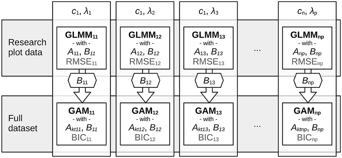
Figure 5. The process of selecting c and λ. First, a range of possible c and λ values was selected. Then, for each combination, a generalized linear mixed model (GLMM) as in Equation 5 was used to fit a mean population, non-sensitive modified Korf curve (cp. Equation 7) to the research plot data to obtain the longitudinal charactersitics of the Hq-age development. Then, the slope Bkt (cp. Equation 7) of each GLMM was set as a fixed coefficient in a generalized additive model (GAM), where the remaining effects, acting upon the intercept Akt, were estimated (see Equation 7b). For each GLMM, the root mean squared error (RMSE) was calculated, for each GAM, the Bayesian Information Criterion (BIC).
We used the root mean squared error (RMSE, Equation 6) as a selection criterion, thus the RMSE was calculated for each GLMM in the grid.
with k and t being indexes for plot and measurement occasion, respectively. n being the number of plots and nk being the number of measurement occasions within plot k. We also considered using the combination leading to the lowest BIC (Schwarz, 1978) as a model selection criterion in the SICM, yet this lead to implausible results concerning the shape of the resulting curve (see ch. 3). Thus this option was discarded and λ and c selection was based solely on the RMSE, albeit advantages of the BIC approach. This will be discussed later on (see ch. 3 and 4).
Once the combination of λ and c, which lead to the minimum RMSE, was found, the step width was decreased to integers for λ and first digit for c, to obtain a more accurate estimate of the ideal parameter combination. The combination of λ and c, which finally resulted in the GLMM with the lowest RMSE, was chosen for further modeling. We also used the corresponding β1 (see Equation 5), which was estimated by the GLMM. From now on, λ and c will refer to said optimal combination.
We then used λ, c and the corresponding β1 to fit a SICM, which estimated the effects acting upon Akt. Once λ and c have been determined, the modified Korf function becomes linear (cp. Equation 7). Thus allowing the use of linear frameworks, such as a GAM. The GAM in turn utilizes regression splines, which enable the flexible modeling of unknown, possibly non-linear effects of the variables on the linear predictor, e.g., optimum curves.
In our case, we used a GAM with a Gaussian family, which further allows for a simultaneous estimation of the mean and the variance of a normal distribution (GAULSS, Wood et al., 2016). Concerning the effects, we used a combination of p-splines for the univariate effects of continous site parameters (Eilers and Marx, 1996), a two dimensional thin plate regression spline (Wood, 2003) as well as effects for categorical site parameters.
with:
such that:
with distribution:
where:
with:
To assess model quality, we calculated the bias:
The SICM was then subject to further adaptions. The spline effects were checked for plausible behavior. If necessary, the corresponding basis dimension was reduced. If the behavior of a spline toward the ends of the data range was influenced by outliers and was not deemed to be biologically sound, the respective outliers were trimmed, such that reasonable effect patterns were achieved. The soil categories, WBC and NBC, also required modifications. Firstly, categories from the Lower Saxony/Schleswig-Holstein scheme are on a rather fine scale, which, in some cases, lead to only few observations per category. Thus they were grouped a priori, by similaritiy regarding the described soil properties, to increase the number of samples per category. For the other mapping schemes, this was not deemed necessary a priori. During the model fit, the effects of WBC and NBC were checked for plausibility and, if necessary, grouped until biologically sound patterns were achieved. However, categories were only grouped if they originated from the same scheme and topology (uplands, lowlands). Moreover, they had to represent comparable soil properties, e.g., waterlogged soils were not mixed with terrestrial ones. This was done to ensure interpretability of the effects as well as differentiated results between the different schemes, topologies and soil properties.
To ensure the stability of the effects, we randomly selected 80% of our data as training data and the remaining 20% as test data. Then, a SICM as in Equation 7c was fitted using the training data and predictions were obtained for the test data. For the latter, we then calculated the RMSE (Equation 6) and the bias (Equation 8) over age. This procedure was repeated 100 times.
First of all, the optimal combination of λ and c was determined by an extensive grid search (cp. 2.2.4), where a GLMM was used to fit a modified Korf curve (see Equation 5) to the research plot data. The aim of the grid search was to minimize the RMSE of said GLMM (see ch. 2.2.4). The optimum values for λ and c, including the corresponding β1, were as follows:
A site index curve using the fixed effects of the corresponding GLMM for β0 and β1 is shown in Figure 6. Since β0, the intercept, is fixed, the resulting shape implicitly resembles a curve under constant environmental conditions, as in our framework the environmental covariates only act upon the intercept (see Equation 7d). Said curve is also compared to yield table curves of Hq over age (Albert et al., 2021), which are seen as a baseline for growth under constant conditions. It is further compared to a site index curve, generated with the combination of λ and c, which lead to a minimal BIC of the corresponding GAM (cp. Figure 5). The latter curve corresponds to constant conditions, as well.
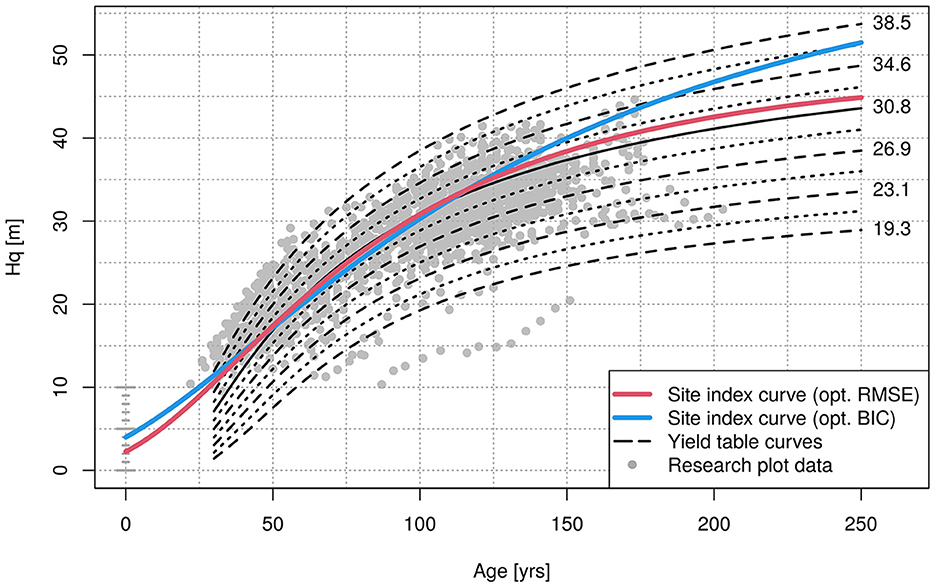
Figure 6. Site index curves for beech under constant conditions. That is, with the fixed effects of the finally selected GLMMs described in 2.2.4 in relation to site index curves (Albert et al., 2021). The red curve corresponds to the GLMM with the lowest RMSE, the blue curve to the GLMM, whose parameters lead to the GAM with the lowest BIC. The numbers on the right indicate the Hq at age 100, 30.8 m has been drawn as a solid line as a reference point.
It can be seen in Figure 6, that the curve leading to the smallest RMSE, which was finally selected, does not start with a height of zero. The modified Korf function is not fixed in the origin, the actual value depends on β0, here it was 3.4, resulting in a Hq of 2.3 m at age zero. While being above the yield table values for younger ages, the curve approaches the pathway of the yield table curves with increasing age. After age 50, the shapes of the curve and the yield table curves show obvious similarity. In contrast, the curve corresponding to the minimum BIC did not follow the pattern of the yield table curves.
Using the aforementioned values of c, λ and β1, i.e., the ones leading to the smallest RMSE, we fitted a SICM as described in 2.2.4. The model itself had a root mean squared error of 3.7 m and an overall bias of 0.10 m. The mean relative deviation of the fitted values from the measured ones was 11.92%. A shortened summary containing the R call can be found in the Supplementary material.
The residuals of the model are shown in Figure 7, plotted over fitted values as well as over age. Note, that fitted values and age are correlated, thus both graphs convey a similar message. Concerning the fitted values (Figure 7A), we found a systematic underestimation for the smallest fitted Hq values of slightly over 2 m. The underestimation decreases continuously until it drops below 1 m at fitted values of 19 m, such that 13% of the fitted values show a bias larger than 1 m. The bias approaches zero at 25 m. For Hq estimates between 25 m and 33 m, i.e., 63% of the fitted values, the bias is negligible. In Figure 7B, it can be clearly seen, that the height development of younger stands is underestimated by the SICM, with a bias of up to 2 m, as well. With increasing age, the bias decreases until it becomes zero at age 70, followed by an overestimation, smaller than 1 m. After age 130, the estimation can be seen as unbiased.
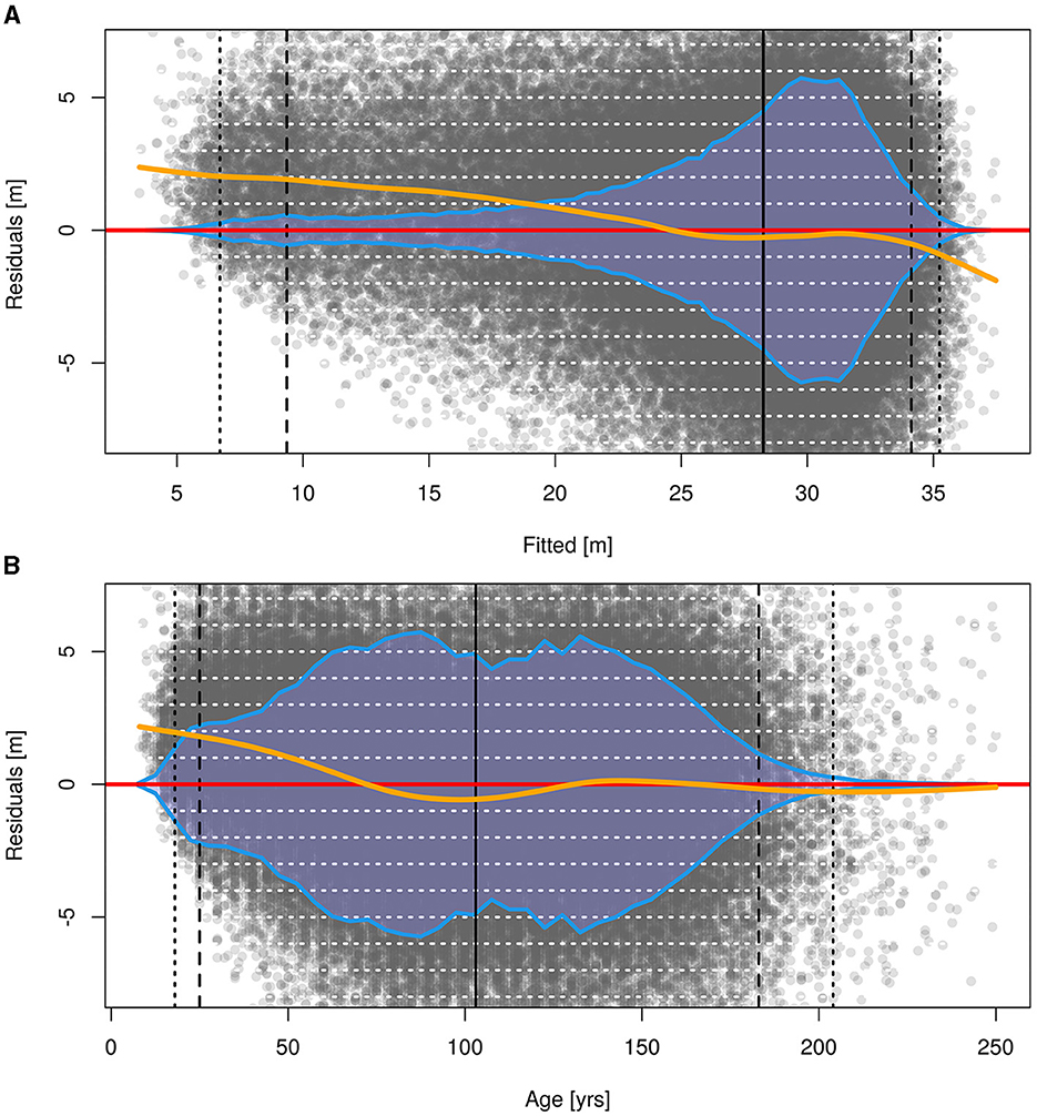
Figure 7. Residuals of the final SICM over fitted values (A) and age (B). The orange line represents a spline to highlight over-/underestimation, the blue area corresponds to the data distribution over the x-axis. The vertical, black lines represent quantiles, i.e., 0.5 and 99.5% (dotted), 2.5 and 97.5% (dashed) as well as the median (solid). Horizontal white lines are placed at each meter. The y-axis ranges from the 0.5% quantile of the residuals to the 99.5% quantile.
The estimated effects for the atmospheric variables with the default spline basis dimension showed generally plausible patterns over large data ranges (cp. Figure 8). However, the basis dimension had to be decreased to reduce the wiggliness and to avoid implausible behavior toward the extremes of the data, which is assumed to be caused by confounding effects. This did not change the general patterns of the effects. As can be seen for the effect for temperature, which initially increased rapidly toward the maximum temperature (Figure 8A). After decreasing the basis dimension, it finally showed an optimum at 2,600°C with moderate decreases to both sides. Below 1,700°C, the decrease got steeper. The pattern of the effect for aridity_veg was generally plausible for most of the data range (Figure 8B). However, due to some extreme outliers >0.35 mm/°C (high precipitation and low temperature, i.e., measurement occasions in the alps), the respective data had to be trimmed to 0.35 mm/°C to avoid unstable behavior of the spline. The final effect size was not as pronounced as the one for tempsum_veg, which is in accordance with the findings of Schmidt (2020) for the effect of precipitation. Moreover, there was no clear optimum, but a plateau between 0.15 and 0.25 mm/°C, with a comparably strong drop toward the left, i.e., drier climates, and a moderate decrease toward the right, i.e., more humid climates. The basis dimension of the spline for Ndep had to be decreased as well to reduce wiggliness, especially toward higher values (Figure 8C). The final effect size was strong compared to the other effects and showed the greatest difference between minimum and maximum effect.
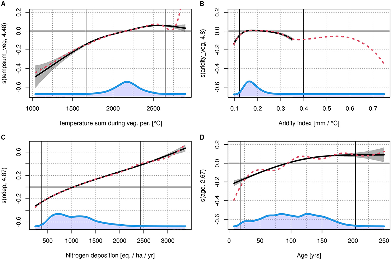
Figure 8. Effects for tempsum_veg (A), aridity_veg (B) and Ndep (C). The last plot (D) shows the effect of age on the standard deviation. All splines are shown with gray confidence bands, the blue area corresponds to the data distribution. Vertical, solid black lines show the 0.5 and 99.5% quantiles of the data. The red, dashed line shows the original spline with default basis dimension.
The behavior of the effect for age, for modeling the standard deviation, originally showed considerable wiggliness (Figure 8D), thus a dimension reduction was applied, as well. Finally, the effect increased in a linear manner from age 0 to age 100, and then approached a steady value. The spatial effect is displayed in the Supplementary material. The two dimensional spline used here is, generally speaking, intended to be rather coarse, as it should only explain large scale spatial influences, e.g., wind pruning (cp. Skovsgaard and Vanclay, 2013). The effect size was only marginal for most of Germany, but became increasingly negative toward the northwest, near the coast of the North Sea.
The effects for the grouped soil categories (cp. ch. 2.2.4) are shown in the Supplementary material. Due to the large variety of possible values for WBC and NBC used within the different states of Germany, it was not possible to unify them across the mapping schemes without distinct loss of sensitivity. Within the mapping schemes, the effects were grouped as described in ch. 2.2.4. If this was not possible, only one effect was estimated for the whole soil type, such as for soils with waterlogging mapped according to the unifying synopsis in the lowlands. Compared to NBC, WBC was more differentiated regarding the soil conditions. It accounts e.g., for groundwater influence or topology, depending on the mapping scheme. Thus the final grouping, across all mapping schemes, consisted of 46 WBC groups, whereas the less complex NBC was grouped into 15 groups.
Generally speaking, the availability of soil water had a positive influence on the site index curve, with stronger effects in the uplands than in the lowlands, where applicable. However, a high level of groundwater or a strong influence of waterlogging showed a negative effect. Effect sizes ranged from 0.07 for terrestric soils with high water capacity in the lowlands, mapped after the unifying synopsis, to −0.26 for dry soils mapped after the scheme of Hessia. The amount of availible nutrients also had a positive effect, with effect sizes ranging from 0.11 for very rich soils, mapped after the Lower-Saxony/Schleswig-Holstein scheme, to −0.04 for very poor soils, mapped after the scheme of Hessia.
We performed model validation as described in ch. 2.2.5, visualized results are shown in the Supplementary material. The model effects estimated on the training data closely resembled the ones from the final SICM, larger deviations were only detected toward the ends of the effects, where less data is available. For all estimated effects, the median of the deviation from the original effect was at most 0.001.
The prediction RMSE ranged from 3.67 to 3.77 m with a median of 3.72 m, whereas the RMSE of the SICM was 3.71 m. When looking at the bias over age, the basic shape of the bias of the SICM is also closely resembled.
To assess the sensitivity of the model, it is necessary to look not only at the effect sizes (see Figure 8), but also at predicted Hq-age-curves. Due to the multiplicative nature of the effects induced by the log-link, the interpretation of the effects is relative and not absolute (Fahrmeir et al., 2013). Thus, sensitivity analysis is performed for the newly developed SICM. Moreover, we compare the results to site index curves predicted with SICMprev, which used a similar model formulation. However, it was solely based on SFTS data, whereas our approach combines SFTS and SSA data.
To compare the resulting curves, we set all numerical variables to their median. The soil categories were set to resemble the mean conditions, i.e., mesotrophic with good water availability. Then, we separately increased tempsum_veg, aridity_veg as well as the nitrogen deposition, respectively, while all other variables were kept constant. Since aridity_veg was not used in SICMprev, we had to use precsum_veg here instead. For each covariate, we generated an equidistant sequence of eight values from the respective 0.5 quantile to the 99.5% quantile. That is, 1,676°C–2,648°C with a median of 2,177°C for tempsum_veg, 0.12 mm/°C–0.4 mm/°C with a median of 0.17 mm/°C for aridity_veg and 282 mm–765 mm with a median of 374 mm for the precipitation sum during the vegetation period. Finally, 379 Equation/ha/a to 2,476 Equation/ha/a with a median of 1,039 Equation/ha/a for Ndep. Coordinates were set to the forest of Göttingen in the center of Germany, where the spatial effect is close to zero. We then used the data to predict Hq development from age 25 to age 200, both with the SICMprev and our newly developed SICM. The predictions of both model versions are then compared, with the yield table curves as a reference (Albert et al., 2021). The results are shown in Figure 9.
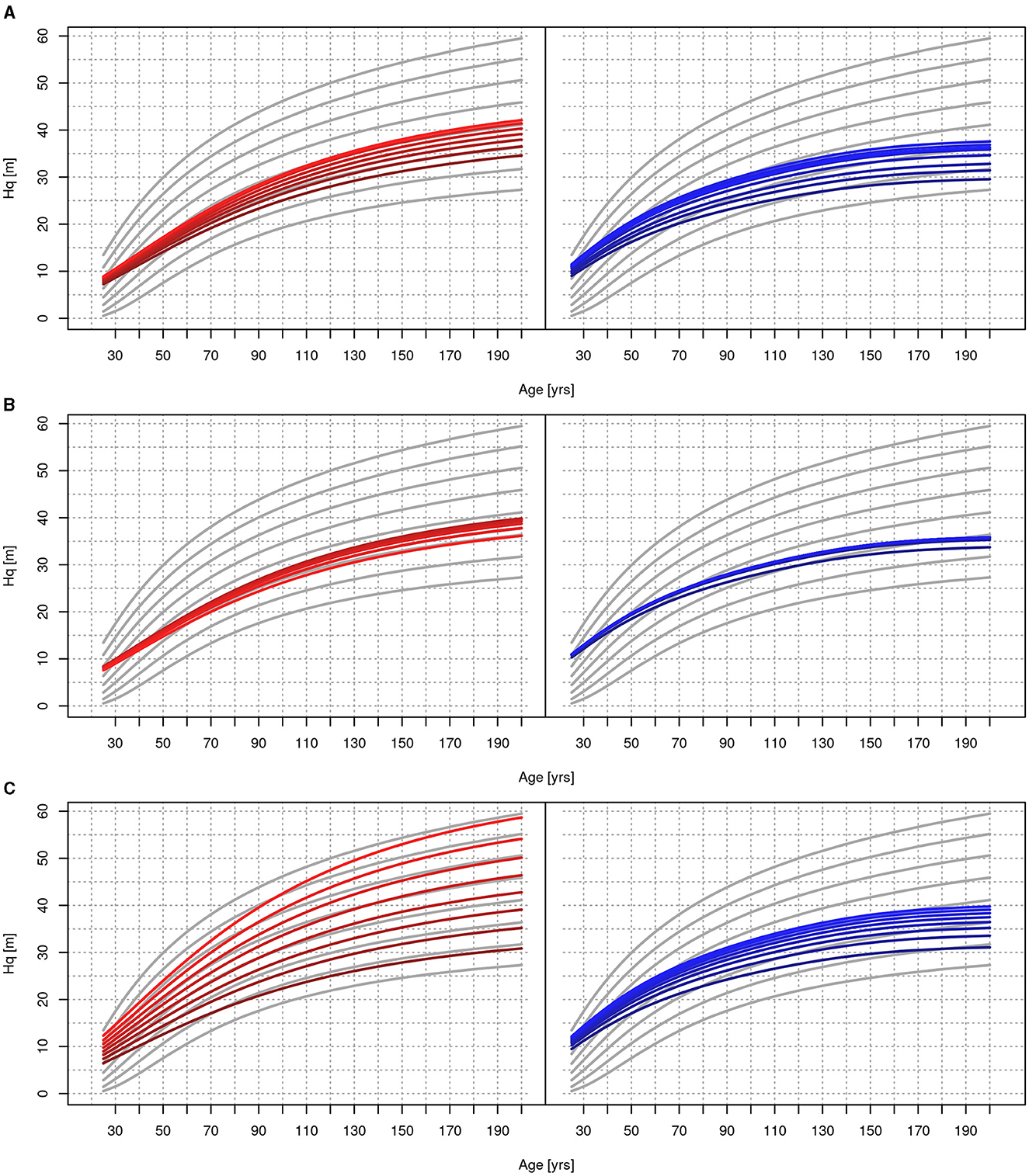
Figure 9. Sensitivity analysis comparing SICM (left, red) with SICMprev (blue, right) by changing temperature sum (A), precipitation sum (B) and nitrogen deposition (C). For each graph, a sequence of eight equidistant values was created for the respective variable, from its 5% quantile (darkest line) to its 95% quantile (brightest line). All other variables were set to the median or modus, for categorical variables. The gray solid and dashed curves are taken from yield tables (Nuske et al., 2022).
Concerning tempsum_veg, we found a difference of 5.5 m at age 100 between the lowest and optimal temperature, for the SICMprev it was 6.6 m. For the SICM we found a difference of 2.7 m for aridity_veg, whereas the SICMprev showed 1.7 m for the precipitation sum during the vegetation period. Note, that the results cannot be compared directly due to the differences in the used variables. Ndep showed the largest effect, as expected, with 20.2 m difference at age 100 in the SICM and 7.1 m in the SICMprev.
Apart from the model comparison, Figure 9 also shows the Hq development over age from the yield tables as a comparison. It should be stressed, that the sensitivity analysis did not calculate the atmospheric variables dynamically, but used one constant value for each Hq-age-curve. Thus assuming site consistency for each curve. It is clearly visible, that the SICM followed the pattern of the yield tables more closely than the SICMprev, especially after age 50. For older stands, the Hq-age pattern predicted by the SICMprev was too flat. The curves estimated by the SICM were steeper, with lower starting values and higher values at age 200.
In this research, we applied substantial advancements to SICMprev (Schmidt, 2020) and the data used for its parameterization. Our goal was to develop a model which can accurately depict forest height development under changing site conditions. The intended use of the model is less as an analytical instrument but mostly as a practical tool for predictions of stand growth under climate change, which is a crucial factor in management (Yue et al., 2016, see also Antón-Fernández et al., 2016; Brandl et al., 2018).
To accurately depict height development under changing site conditions, a number of environmental factors has to be accounted for in the analysis, e.g., atmospheric and geographic variables as well as soil parameters (cp. Seynave et al., 2005; Bontemps and Bouriaud, 2014; Yue et al., 2016; Antón-Fernández et al., 2023).
Concerning the atmospheric data, we deemed air temperature, precipitation and nitrogen deposition as the most influential factors (cp. Yue et al., 2016). Moreover, the direct use of atmospheric data, instead of topographical indicators, such as elevation, enables the use of the model for predictions (cp. Bontemps and Bouriaud, 2014). Compared to other studies, our data has a finer spatial and temporal scale. Concerning the spatial scale, the fine resolution of the used 50 m × 50 m grid allows for nuanced values in changing terrain, e.g., in uplands. This would not be possible with the coarse resolution of the raw data (cp. Skovsgaard and Vanclay, 2013; Bontemps and Bouriaud, 2014), e.g., the data of WorldClim with a resolution of 1 km (Brandl et al., 2018). Moreover, the fine spatial resolution of our data allowed us, to correct the temperature for aspect and slope, i.e., decreasing the temperature on northern slopes and increasing it on a southern one. Thus accounting for the topology induced differences in radiation influencing air temperature. Other studies used a similar temperature correction, e.g., Sterba et al. (1995) used aspect and slope as coefficients in a forest productivity model, and Running et al. (1987) corrected temperature for aspect and slope when simulating forest evapotranspiration and photosynthesis. However, to our knowledge, said correction was not implemented in the context of modeling stand height development. The fine temporal resolution of the atmospheric data enabled further advancements. First of all, the annually determined vegetation period, used for temperature and precipitation, allows for distinct values for each year, depending on the conditions. Nitrogen was summed up annually. We then calculated a weighted mean of those sums over stand life, utilizing growth increment functions as a weight. This had two advantages: First, this dynamic approach is more realistic than a rather static approach used in other studies, where a fixed vegetation period (cp. Yue et al., 2016) or seasonal values (cp. Dănescu et al., 2017; Brandl et al., 2018; Antón-Fernández et al., 2023) have been used. Second, the weights allow the same environmental conditions to exert different influences on stand height, depending on the age and the corresponding growing phase they occurred in. Both the weighted mean and the temperature correction were not implemented in SICMprev. Moreover, the weighted mean has not been utilized in other previous approaches for modeling site index. Those novelties will lead to more detailed and feasible predictions, better representation of the physical and biological processes influencing stand growth and lastly increase prediction precision.
After applying the transformations to the variables, the correlation between the covariates was weak (see Figure 4), with the exception of Ndep and stand age as well as, to a lower extent, tempsum_veg and aridity_veg. However, we found, that the correlation of Ndep is rather with the germination year. The causality of this correlation is the short time span during which the inventories, which make up the largest part of the data, were taken. They were only conducted between 1987 and 2021, i.e., a period of 34 years, whereas stand age ranged up to 250 years in our data. This lead to a high correlation of age and germination year (−0.98). The correlation between the latter and Ndep is, in turn, a logical consequence of rising nitrogen depositions over the last century (Schöpp et al., 2003). Apart from Ndep and stand age, the only relevant correlation was between tempsum_veg and aridity_veg, which is a logical consequence of the former being used to calculate the latter. Yet we argue, that aridity_veg is a useful addition to the model, since it better accounts for arid climates than precipitation alone.
We also extended our data concerning the soil categories, WBC and NBC, such that both variables are now present for 89% of the measurement occasions. Thus contrasting used datasets of other studies, where soil variables were not available and could not be included (cp. e.g., Brandl et al., 2018; González-Rodríguez and Di'eguez-Aranda, 2021b). Soil properties are characterized by a high spatial variability (Skovsgaard and Vanclay, 2013) and showed a comparably large influence on stand height growth development in our analysis, thus highlighting their importance for both prediction accuracy and sensitivity, and avoiding confouding effects on time-varying climate and deposition parameters. We used three different soil mapping schemes, i.e., Lower Saxony/Schleswig-Holstein, Hessia and the unifying synopsis for Germany. The latter was only used, when no other data were present. The use of the state specific schemes, where possible, avoided the translation of the values into the unifying synopsis. Such a procedure would be accompanied by a loss of information, since the categories do not convey the same meanings and cannot be translated directly. Moreover, the Lower Saxony/Schleswig-Holstein scheme is substantially more differentiated. Within our dataset, we recorded 106 different values for WBC and 13 for NBC for said scheme, whereas the unifying synopsis only offers 19 possible values for WBC and 6 for NBC. By keeping the schemes, we therefore achieved more distinct estimates for the different soil types, which will lead to more precise predictions in the application. Moreover, it enables the direct interpretation of the results by the respective state forest enterprises, which are used to their respective soil mapping schemes. Finally, we used an unknown category (separated into up- and lowlands) for all plots, where no soil mapping was present at all. We therefore could still include the remaining data (tempsum_veg, Ndep, etc.) for the estimation of the corresponding effects. Furthermore, this enables the application of the model on stands without soil mapping data.
Concerning dendrometry, we generated a unique dataset containing measurements from both inventory data, representing SFTS, and research plot data, representing SSA. To our knowledge, we are the first to combine these two approaches for site-index modeling on a large scale. Other research used either SSA (Yue et al., 2016; Dănescu et al., 2017; González-Rodríguez and Diéguez-Aranda, 2021a) or SFTS data (Seynave et al., 2005; Antón-Fernández et al., 2016; Brandl et al., 2018), a substantial combination of the two has not been realized yet.
The inventory data consists of NFI, EFI, and CI data. Since these inventories are a representative sample of the respective area, with the NFI covering all of Germany, this part of the data represents a broad range of environmental conditions, under which beech trees grow in Germany (cp. Figure 1), with the exception of very rare conditions. However, there were on average only 1.5 measurements occasions per plot, thus the longitudinal characteristics of stand growth development cannot be assessed with this data. To obtain a model with a sound longitudinal trend, it was crucial to include data with a broader temporal scale (cp. Aertsen et al., 2012; Damgaard, 2019). We used research plot data, which is characterized by a high number of repeated measurements on a large number of trees, thus the resulting Hq values accurately depict stand growth development over time. Hence we argue, that the research plots closely depict the true growth potential of the stand over time. This data was not used in SICMprev, its inclusion presents a substantial improvement which allows for a realistic estimate of the basic shape of the curve and therefore estimation of site sensitive Hq curves with a feasible development over age.
One disadvantage of using the Hq, is its sensitivity to thinning. Using a top stand height, e.g., the mean height of the 20% strongest trees, would have circumvented that problem, at least for most thinning types. However, the top height of a stand does not equal the one calculated from a sample, since the aforementioned upper quantile depends on the distribution of the respective data and thus depends on the variance of the reference unit (stand vs. sample) (Schmidt, 2020).
We based our model on a modified version of the Korf curve, which was originally developed by Lappi (1997) as a longitudinal height-diameter curve and has been modified to depict Hq-age relationships. The same basis was also used by SICMprev and has several advantages: Despite its simplicity, it inhibits a high flexibility and can mimic the shape of other growth curves. Another advantage over other growth curves is its partial linearity. After c and λ have been set, the parameters Akt and Bkt can be estimated within a linear framework. This ensures, that the solution found is indeed optimal and avoids computational issues or iterative solutions (cp. Yue et al., 2016). Moreover, the clear biological interpretation of Akt and Bkt (cp. Lappi, 1997) allows for a direct evaluation and comparison of parameter estimates. The only disadvantages are, that it does not necessarily start in the origin, which lead to non-zero heights at age zero. It also does not have an asymptome, which, however, did not pose a problem in our research. Actually it is advantageous if an effect of Ndep should be estimated from data where high Ndep-values occur only in young stands (as is the case in our data). Tests with different growth curves, which included an asymptote, resulted in a negative effect of Ndep on the asymptote, caused by the unbalanced data. Moreover, the pattern of the yield table curves can be replicated even until age 250 (see Figure 6), indicating that height growth is indeed not completed.
The modeling framework we chose for the final model is a GAM, which utilizes the GAULSS family (Wood et al., 2016; Wood, 2017). A GAM offers several advantages: Firstly, the use of splines allows a highly flexible modeling of effect shapes, including optimum curves, which is essential for the intended use. Moreover, due to the used modified Korf function, effects can be interpreted directly. This distinguishes our approach e.g., from machine learning methods, such as boosted regression trees (González-Rodríguez and Di'eguez-Aranda, 2021b; Antón-Fernández et al., 2023), where a direct interpretation of the parameters is not feasible. The effects can also be estimated directly. This contrasts e.g., multi-level models (Nothdurft et al., 2012), where separate estimates from different models are needed. Thus making effect interpretation possibly non-trivial, as a hierarchy of effects has to be interpreted simultaneously.
One problem with SICMprev was the longitudinal pattern of its predicted site index curves. That is, when setting all environmental conditions constant over stand life, one would assume the model prediction to correspond to the shape defined by yield tables, which follow empirical data and are assumed to depict tree growth under such conditions. However, the resulting curve predicted by SICMprev was too flat (see Figure 9). Moreover, we observed the same behavior when comparing SICMprev to the long time series data of our research plots. We argue, that this is mostly due to the fact, that the longitudinal charactersitics of the inventory data were not accounted for in SICMprev. To account for this longitudinal structure, as well as the environmental influences, we tried fitting a mixed GAM to our dataset. This approach was tested in multiple attempts, however, the model did not converge. Moreover, the number of measurement occasions within the inventory data is low, with 57% of the plots only having one measurement. Combined with the comparably short time span, in which the measurements were taken, it is questionable whether this approach would lead to a biologically sound curve. Another issue might be the absence of SSA data, SICMprev only used SFTS data, i.e., inventories. Using our dataset, we could determine, that the inventories resulted, on average, indeed in a flatter site index curve than the research plots (a figure comparing the two can be found in the Supplementary material). We argue, that this could be due to the differences in management on inventory plots vs. research plots. Especially target diameter harvesting, usually being performed in standard forest management, i.e., inventory plots, will lead to stagnating Hq values. However, this hypotheses cannot be tested due to the low number of successive measurement occasions per plot in the inventories. Another reason for the flatter curve might be in the selection of sites, since research plots are usually placed on homogenous terrain and will therefore not be found, e.g., on steep hills. We also considered a difference in environmental conditions between research plots and inventory data as a factor. However, when looking at Table 1, it is clear, that the data mainly differs in its extremes. For example, the minimum temperature sum was 1,037 °C for the inventory data and 1,770 °C for the research plots, yet the 2.5% quantiles only differ by 21 °C. The remaining quantiles, except for the maximum, are also reasonably close in value. Similar patterns can be observed for the precipitation as well, only nitrogen deposition was noticably higher for the research plot data. To further investigate, we computed separate modified Korf curves for inventory plots, which are no more than 25 km away from the next research plot. The results did not change substantially. Thus environmental factors could be excluded as an explanation, as well. Having examined the different possibilities, we argue, that the driving factor behind the predicted Hq-age patterns of SICMprev, is most likely the aforementioned problem assessing the longitudinal properties of the inventories.
As a solution, we derived a hierarchical set of models. We based the estimation of λ, c and Bkt on the research plots, which we assume to closely depict the true growth potential and pattern, and the estimation of Akt on the full dataset. Thus, the research plots defined the basic shape of the curve while the effects acting upon the level of the curve, Akt, could still be estimated with the full dataset. We therefore combined a SSA with a SFTS approach in a hierarchical model (cp. Damgaard, 2019). That is, we combined the longitudinal properties of the research plots with the broad environmental conditions covered by the inventories. To our knowledge, this approach presents a novelty in site index modeling.
When deciding, which combination of the coefficients λ, c and Bkt to use for the final model, we investigated two possible criteria: (1) The RMSE of the GLMM, which estimated the coefficients from research plot data, or (2) the BIC of the GAM, which used the coefficients from the GLMM to estimate a SICM for the full dataset (cp. Figure 5). As it can be seen in Figure 6, there are substantial differences in the curves, depending on the used criterium. It should be stressed, that the driving factor behind said differences is the used combination of λ and c, which defines the underlying shape of the curve. Both curves were fitted using research plot data only.
When fitting the SICM with the coefficients λ, c and Bkt, which lead to the minimal BIC, an unbiased prediction for the full dataset was achieved. However, the shape of the resulting curve (see Figure 6) was deemed too straight and not realistic. Moreover, when setting the environmental conditions constant, this model did not follow the pattern of the yield tables, which are assumed to depict stand growth under such conditions. We therefore chose the RMSE as a selection criterium, due to the sound pattern of the corresponding site index curve.
However, the resulting estimations of the SICM were no longer unbiased. Especially for stands younger than 50 years, or fitted values below 19 m, respectively, there was a noticable, systematic underestimation of more than 1 m (cp. Figure 7). However, < 13% of the measurements were taken before age 50, hence 87% of the data can be estimated with a bias of < 1 m. Moreover, there is no substantial bias for ages >120. Though the bias is not extremely severe, it should be taken into account during the application, especially since model validation indicated, that the bias will not change substantially for predictions. Further research is needed to fully grasp the causality behind said bias and thereafter investigate possible solutions. For example, trying different functions for Hq-age development, adding covariates or modifying their processing.
The effects estimated by the model also showed plausible patterns. Their general shape did not change relevantly during model validation, albeit being fitted on only 80% of the data. Thus indicating the robustness of the results.
We can see an optimum for tempsum_veg and aridity_veg, with clear negative tendencies toward the extremes. The effect for the aridity was comparably weak, however, this is in accordance with the findings of Schmidt (2020) for precipitation. Brandl et al. (2018) also found a weaker effect of precipitation compared to temperature, though generally larger in magnitude. The aridity index itself, which is also used in different formulations in other modeling approaches, e.g., by Yue et al. (2016), is another advancement over SICMprev: Precipitation is summed over the vegetation period, which will, in turn, extend with rising temperatures. Thus, a decrease in daily precipitation will not necessarily lead to a decreasing precipitation sum during the vegetation period. This has to be considered when predicting stand growth under climate change. The aridity index tackles this issue by directly relating precipitation and temperature, and thus leading to more reliable predictions. Another considerable difference from SICMprev is the direct modeling of the nitrogen effect. Schmidt (2020) found considerable correlation between the nitrogen deposition and the stand age, thus a model was used here to normalize the nitrogen deposition with the expected value over age and to reduce correlation. Our data holds the same property (see Figure 4). However, we found that the correlation is rather with the germination year than the age, as explained above. Yet including an effect for the germination year was not feasible. When applying the model for projections, one would need to extrapolate said effect without having any logically sound way to asses, or verify, the future development of an effect for germination year. Thus regularization approaches, such as boosting (cp. Antón-Fernández et al., 2023), were also not feasible. It was therefore not possible to separate the influences of the germination year and/or the age and the nitrogen deposition. This problem is well known in epidemiology as the age-period-cohort problem, where setting two of the three defines the third, such that separating the effects is hardly possible (cp. Keyes and Li, 2011). However, including nitrogen deposition was still necessary, as the resulting effect captures one of the main drivers of change in site quality (cp. Skovsgaard and Vanclay, 2013).
Finally, the GAULSS family used in the GAM allows a simultaneous estimation of the standard deviation (Wood et al., 2016), which we modeled as a function of age. The resulting spline increases until age 100 and flattens out afterwards. This behavior was expected, since the absolute value of the standard deviation is correlated with Hq. The estimated standard deviation can be used in application to calculate confidence intervals alongside the mean, thus supplying a measure of uncertainty. This is of great value, e.g., in economical calculations or management planning. Finally, the chosen framework allows a direct modeling of stand height at a given age, instead of modeling the site index at a specific age (cp. e.g., Antón-Fernández et al., 2016; Yue et al., 2016). Hence, we can predict Hq development for the whole stand life without additional methods or functions.
We finally argue, that predicting the correct development of stand height over age is more valuable than a fully unbiased prediction. By combining the longitudinal properties of the research plots with the broad range of environmental conditions covered by the inventory data, we were able to create a SICM which estimates height growth curves with realistic longitudinal properties derived from SSA data, while still incorporating the information of the broad SFTS data. Moreover, the model does not require initial dendrometry data. This separates our approach e.g., from Yue et al. (2016), where an initial site index is needed for the model. Antón-Fernández et al. (2023) also recommend to use their model rather for predicting site index changes, which are added to a recent site index measurement. However, climate change will also require a change in tree species on several sites (Albert et al., 2017). Thus predicting height growth development of not yet established tree species is essential for future forest management questions (Bontemps and Bouriaud, 2014).
We introduced a site index curve model for beech, which portrays the prototype for a new generation of models. As of now, we were able to include several, substantial advancements over SICMprev which lead to higher differentiated and longitudinally more sound predictions. However, there are still some issues which require further research. Considering the weighted mean of the atmospheric data, we will investigate the effect of different height increment functions, i.e., different weights, on prediction quality and bias. Furthermore, we will examine the influence of sulfur depositions on height development, with sulfur being a counterweight to increasing nitrogen depositions. Sulfur depositions in Germany have halved between 2000 and 2015 (Schaap et al., 2018), this decrease might be an important factor, especially for younger stands. That is, where the bias was most critical. However, the respective data is not available to us yet. We will also investigate the possible inclusion of further covariates, such as topographical or environmental indicators. Moreover, we consider fitting models for the development of top height over age. Thus overcoming the stronger influence of forest management on the Hq.
Finally, we will apply the methodology described here, with possible further advancements, to also develop models for additional species. These models will provide climate sensitive predictions for height development with a feasible pattern over age for different tree species, which thrive in a variety of environmental conditions. Moreover, we will fit a mixed model, which can then be utilized to estimate random effects for the site index curves with measured stand heights (cp. Mehtätalo, 2004; Schmidt, 2020). In combination with the SICM, this will enable robust, climate and site sensitive predictions of stand height development, calibrated with dendrometry of the respective stand. Thus greatly increasing prediction accuracy (Schmidt, 2020).
Concerning the application of the SICM, the results can be used in forest planning to assess wood production, carbon storage or, as an auxiliary parameter, for predictions of biotic and abiotic risks, such as windfall. As our approach does not require initial site index measurements, simulations can be carried out independently of structure and species composition of the current stand. This also enables the use in forest simulators, such that climate sensitive simulations for potential stands can be achieved. As noted e.g., by Fuchs et al. (2022), this would overcome the often used assumption of constant site conditions and allow the simulation of multiple stands. Moreover, Hq estimations of our model combined with site parameters will be used in a forest productivity model. As Bontemps and Bouriaud (2014) pointed out, the link between stand height development and productivity is doubtful. By using a separate model, productivity does not have to be infered from yield tables, which no longer correctly depict the relationship between height and productivity, e.g., due to increased nitrogen deposition, but can be estimated directly. Thus overcoming aforementioned criticism.
The datasets presented in this article are not readily available because (1) the contents of the used inventory data are confidential, especially the location of the plots, and (2) the data for modeling nitrogen deposition was supplied by the Federal Environment Agency (UBA), which did not grant permission for distribution. Requests to access the datasets should be directed at: JS, amFuLnNjaGlja0Budy1mdmEuZGU=.
JS and MS contributed to conception and design of the study. JS organized the database and developed the model. JS, MA, and MS jointly discussed the stages of the modeling process. JS and MA wrote the first draft of the manuscript. All authors contributed to manuscript revision, read, and approved the submitted version.
This research was carried out within the Research Training Group 2300 EnriCo, funded by the DFG (Funding grant 316045089). We acknowledge support by the Open Access Publication Funds of the Göttingen University.
We thank Holger Sennhenn-Reulen for extensive help with model development and statistical questions, Kai Staupendahl for functionalizing the growth curves and developing the basis of the stratum separator, Thorsten Zeppenfeld for modeling climatic data, Bernd Ahrends for modeling N-deposition and helping with the description of said modeling and Hans Hamkens for processing soil data. We further thank the state forest enterprises of Hessia, Lower-Saxony, Saxony-Anhalt and Schleswig-Holstein for supplying dendrometrical and soil mapping data. We also thank two reviewers for their useful comments and suggestions.
The authors declare that the research was conducted in the absence of any commercial or financial relationships that could be construed as a potential conflict of interest.
All claims expressed in this article are solely those of the authors and do not necessarily represent those of their affiliated organizations, or those of the publisher, the editors and the reviewers. Any product that may be evaluated in this article, or claim that may be made by its manufacturer, is not guaranteed or endorsed by the publisher.
The Supplementary Material for this article can be found online at: https://www.frontiersin.org/articles/10.3389/ffgc.2023.1201636/full#supplementary-material
Adler, P. B., Dalgleish, H. J., and Ellner, S. P. (2012). Forecasting plant community impacts of climate variability and change: when do competitive interactions matter? J. Ecol. 100, 478–487. doi: 10.1111/j.1365-2745.2011.01930.x
Aertsen, W., Janssen, E., Kint, V., Bontemps, J.-D., Van Orshoven, J., Muys, B., et al. (2014). Long-term growth changes of common beech (Fagus sylvatica L.) are less pronounced on highly productive sites. For. Ecol. Manage. 312, 252–259. doi: 10.1016/j.foreco.2013.09.034
Aertsen, W., Kint, V., Muys, B., and Orshoven, J. V. (2012). Effects of scale and scaling in predictive modelling of forest site productivity. Environ. Model. Softw. 31, 19–27. doi: 10.1016/j.envsoft.2011.11.012
Ahrends, B., Fortmann, H., and Meesenburg, H. (2022). The influence of tree species on the recovery of forest soils from acidification in lower Saxony, Germany. Soil Syst. 6, 40. doi: 10.3390/soilsystems6020040
Ahrends, B., Schmitz, A., Prescher, A.-K., Wehberg, J., Geupel, M., Andreae, H., et al. (2020). Comparison of methods for the estimation of total inorganic nitrogen deposition to forests in Germany. Front. For. Global Change 3, 103. doi: 10.3389/ffgc.2020.00103
Albert, M., Nagel, J., Schmidt, M., Nagel, R.-V., and Spellmann, H. (2021). Data from: Eine neue Generation von Ertragstafeln für Eiche, Buche, Fichte, Douglasie und Kiefer. Zenodo. doi: 10.5281/zenodo.6343906
Albert, M., Nagel, R.-V., Nuske, R. S., Sutmöller, J., and Spellmann, H. (2017). Tree species selection in the face of drought risk—uncertainty in forest planning. Forests 8, 363. doi: 10.3390/f8100363
Albert, M., and Schmidt, M. (2010). Climate-sensitive modelling of site-productivity relationships for Norway spruce (Picea abies (L.) Karst.) and common beech (Fagus sylvatica L.). For. Ecol. Manage. 259, 739–749. doi: 10.1016/j.foreco.2009.04.039
Albrecht, A., Duran-Rangel, C., Kändler, G., Schmidt, M., Yue, C., and Kohnle, U. (2017). “Evaluierung verschiedener klimasensitiver Bonitätsmodelle für Fichte,” in Jahrestagung der Sektion Ertragskunde, DVFFA, eds U. Kohnle and J. Klädtke (Freiburg: Selbstverlag FVA Baden-Württemberg), 59–69.
Álvarez González, J. G., Cañellas, I., Alberdi, I., Gadow, K. V., and Ruiz-González, A. D. (2014). National Forest Inventory and forest observational studies in Spain: applications to forest modeling. For. Ecol. Manage. 316, 54–64. doi: 10.1016/j.foreco.2013.09.007
Alveteg, M., Walse, C., and Warfvinge, P. (1998). Reconstructing historic atmospheric deposition and nutrient uptake from present day values using MAKEDEP. Water Air Soil Pollut. 104, 269–283. doi: 10.1023/A:1004958027188
Antón-Fernández, C., Hauglin, M., Breidenbach, J., and Astrup, R. (2023). Building a high-resolution site index map using boosted regression trees: the Norwegian case. Can. J. For. Res. 53, 416–429. doi: 10.1139/cjfr-2022-0198
Antón-Fernández, C., Mola-Yudego, B., Dalsgaard, L., and Astrup, R. (2016). Climate sensitive site index models for Norway. Can. J. For. Res. 99, 1–33. doi: 10.1139/cjfr-2015-0155
Auger-Méthé, M., Newman, K., Cole, D., Empacher, F., Gryba, R., King, A. A., et al. (2021). A guide to state–space modeling of ecological time series. Ecol. Monogr. 91, 1–38. doi: 10.1002/ecm.1470
Benning, R., Ahrends, B., Amberger, H., Danigel, J., Gauer, J., Hafner, S., et al. (2020). The Soil Profile Database for the National Forest Inventory Plots in Germany Derived from Site Survey Systems. Göttingen.
Boisvenue, C., and Running, S. W. (2006). Impacts of climate change on natural forest productivity - evidence since the middle of the 20th century. Glob. Chang. Biol. 12, 862–882. doi: 10.1111/j.1365-2486.2006.01134.x
Bontemps, J.-D., and Bouriaud, O. (2014). Predictive approaches to forest site productivity: recent trends, challenges and future perspectives. Forestry 87, 109–128. doi: 10.1093/forestry/cpt034
Brandl, S., Mette, T., Falk, W., Vallet, P., Rötzer, T., and Pretzsch, H. (2018). Static site indices from different national forest inventories: harmonization and prediction from site conditions. Ann. For. Sci. 75, 1–17. doi: 10.1007/s13595-018-0737-3
Damgaard, C. (2019). A critique of the space-for-time substitution practice in community ecology. Trends Ecol. Evol. 34, 416–421. doi: 10.1016/j.tree.2019.01.013
Dănescu, A., Albrecht, A. T., Bauhus, J., and Kohnle, U. (2017). Geocentric alternatives to site index for modeling tree increment in uneven-aged mixed stands. For. Ecol. Manage. 392, 1–12. doi: 10.1016/j.foreco.2017.02.045
Eilers, P. H. C., and Marx, B. D. (1996). Flexible smoothing with B-splines and penalties. Stat. Sci. 11, 89–102. doi: 10.1214/ss/1038425655
Engardt, M., Simpson, D., Schwikowski, M., and Granat, L. (2017). Deposition of sulphur and nitrogen in Europe 1900–2050. Model calculations and comparison to historical observations. Tellus B Chem. Phys. Meteorol. 69, 1328945. doi: 10.1080/16000889.2017.1328945
Fahrmeir, L., Kneib, T., Lang, S., and Marx, B. (2013). Regression. Berlin: Springer. doi: 10.1007/978-3-642-34333-9
Federal Ministry of Food Agriculture (2016). Ergebnisse der Bundeswaldinventur 2012. Available online at: https://www.bundeswaldinventur.de (accessed March 29, 2023).
Fuchs, J. M., Hittenbeck, A., Brandl, S., Schmidt, M., and Paul, C. (2022). Adaptation strategies for spruce forests—economic potential of bark beetle management and Douglas fir cultivation in future tree species portfolios. Forestry 95, 229–246. doi: 10.1093/forestry/cpab040
García, O. (1994). The state-space approach in growth modelling. Can. J. For. Res. 24, 1894–1903. doi: 10.1139/x94-244
González-Rodríguez, M. Á., and Diéguez-Aranda, U. (2021a). Delimiting the spatio-temporal uncertainty of climate-sensitive forest productivity projections using support vector regression. Ecol. Indic. 128, 107820. doi: 10.1016/j.ecolind.2021.107820
González-Rodríguez, M. Á., and Diéguez-Aranda, U. (2021b). Rule-based vs parametric approaches for developing climate-sensitive site index models: a case study for Scots pine stands in northwestern Spain. Ann. For. Sci. 78, 1–14. doi: 10.1007/s13595-021-01047-2
HessenForst (2017). Hessische Waldbaufibel: Grundsätze und Leitlinien zur Naturnahen Wirtschaftsweise im Hessischen Staatswald. Kassel: Druckerei Boxan.
Hurlbert, S. H. (1984). Pseudoreplication and the design of ecological field experiments. Ecol. Monogr. 54, 187–211. doi: 10.2307/1942661
Keyes, K. M., and Li, G. (2011). “Age–period–cohort modeling,” in Injury Research, eds G. Li, and S. Baker (Boston, MA: Springer), 409–426. doi: 10.1007/978-1-4614-1599-2_22
Klesse, S., DeRose, R. J., Babst, F., Black, B. A., Anderegg, L. D. L., Axelson, J., et al. (2020). Continental-scale tree-ring-based projection of Douglas-fir growth: testing the limits of space-for-time substitution. Glob. Chang. Biol. 26, 5146–5163. doi: 10.1111/gcb.15170
Koch, N. E., and Skovsgaard, J. P. (1999). Sustainable management of planted forests: some comparisons between Central Europe and the United States. New For. 17, 11–22. doi: 10.1023/A:1006520809425
Kohnle, U., Albrecht, A., Lenk, E., Ohnemus, K., and Yue, C. (2014). Growth trends driven by environmental factors extracted from long term experimental data in southwest Germany. Allg. Forst Jagdztg. 185, 97–117.
Korf, V. (1939). Príspevek k matematické definici vzrustového zákona hmot lesních porostu. Lesnicka Prace 18, 339–356.
Lindner, M., Fitzgerald, J. B., Zimmermann, N. E., Reyer, C., Delzon, S., van der Maaten, E., et al. (2014). Climate change and European forests: what do we know, what are the uncertainties, and what are the implications for forest management? J. Environ. Manage. 146, 69–83. doi: 10.1016/j.jenvman.2014.07.030
Mehtätalo, L. (2004). A longitudinal height–diameter model for Norway spruce in Finland. Can. J. For. Res. 34, 131–140. doi: 10.1139/x03-207
Menzel, A. (1997). Phänologie von Waldbäumen unter sich ändernden Klimabedingungen - Auswertung der Beobachtungen in den Internationalen Phänologischen Gärten und Möglichkeiten der Modellierung von Phänodaten. München: Forstliche Forschungsberichte München. p. 164.
Monserud, R. A., Huang, S., and Yang, Y. (2006). Predicting lodgepole pine site index from climatic parameters in Alberta. For. Chron. 82, 562–571. doi: 10.5558/tfc82562-4
Nagel, J., Spellmann, H., and Pretzsch, H. (2012). Zum Informationspotenzial langfristiger forstlicher Versuchsflächen und periodischer Waldinventuren für die waldwachstumskundliche Forschung. Allg. Forst Jagdztg. 183, 111–116.
NFP, N. (2007). Forstliche Standortsaufnahme – Geländeökologischer Schätzrahmen. Anwendungsbereich: Mittelgebirge, Bergland und Hügelland. Wolfenbüttel, 12.
NFP, N. (2009). Forstliche Standortsaufnahme – Geländeökologischer Schätzrahmen. Anwendungsbereich: Pleistozänes (Diluviales) Flachland. Wolfenbüttel, 14.
Nord-Larsen, T., and Johannsen, V. K. (2007). A state-space approach to stand growth modelling of European beech. Ann. For. Sci. 64, 365–374. doi: 10.1051/forest:2007013
Nothdurft, A., Wolf, T., Ringeler, A., Böhner, J., and Saborowski, J. (2012). Spatio-temporal prediction of site index based on forest inventories and climate change scenarios. For. Ecol. Manage. 279, 97–111. doi: 10.1016/j.foreco.2012.05.018
Nuske, R. (2017). Data from: vegperiod: Determine Thermal Vegetation Periods. Zenodo. doi: 10.5281/zenodo.1466541
Nuske, R., Staupendahl, K., and Albert, M. (2022). et.nwfva: Forest Yield Tables for Northwest Germany and their Application. R package version 0.1.0.900.
Pickett, S. T. (1989). “Space-for-time substitution as an alternative to long-term studies,” in Long-Term Studies in Ecology, ed G. E. Likens (New York, NY: Springer-Verlag), 110–135. doi: 10.1007/978-1-4615-7358-6_5
Pretzsch, H. (1992). Zunehmende Unstimmigkeiten zwischen erwartetem und wirklichem Wachstum unserer Waldbestände. Forstwissensch. Centralbl. 111, 366–382. doi: 10.1007/BF02741687
Pretzsch, H., Biber, P., Schütze, G., Uhl, E., and Rötzer, T. (2014). Forest stand growth dynamics in Central Europe have accelerated since 1870. Nat. Commun. 5, 1–10. doi: 10.1038/ncomms5967
Pretzsch, H., del Río, M., Biber, P., Arcangeli, C., Bielak, K., Brang, P., et al. (2019). Maintenance of long-term experiments for unique insights into forest growth dynamics and trends: review and perspectives. Eur. J. For. Res. 138, 165–185. doi: 10.1007/s10342-018-1151-y
R Core Team (2021). R: A Language and Environment for Statistical Computing. Vienna: R Foundation for Statistical Computing.
Running, S. W., Nemani, R. R., and Hungerford, R. D. (1987). Extrapolation of synoptic meteorological data in mountainous terrain and its use for simulating forest evapotranspiration and photosynthesis. Can. J. For. Res. 17, 472–483. doi: 10.1139/x87-081
Schaap, M., Hendriks, C., Kranenburg, R., Kuenen, J., Schlutow, A., Nagel, H.-D., et al. (2018). PINETI-3: Modellierung atmosphärischer Stoffeinträge von 2000 bis 2015 zur Bewertung der "okosystem-spezifischen Gefährdung von Biodiversität durch Luftschadstoffe in Deutschland. Technical report, Dessau-Roßlau: Umweltbundesamt (UBA).
Schmidt, M. (2010). “Ein standortsensitives, longitudinales Höhen-Durchmesser-Modell als eine Lösung für das Standort-Leistungs-Problem in Deutschland,” in Jahrestagung der Sektion Ertragskunde, DVFFA, ed J. Nagel (Göttingen), 131–152.
Schmidt, M. (2020). Standortsensitive und kalibrierbare bonitätsfächer: wachstumspotenziale wichtiger baumarten unter klimawandel. Allg. Forst Jagdztg. 190, 136–160.
Schöpp, W., Posch, M., Mylona, S., and Johansson, M. (2003). Long-term development of acid deposition (1880–2030) in sensitive freshwater regions in Europe. Hydrol. Earth Syst. Sci. 7, 436–446. doi: 10.5194/hess-7-436-2003
Schwarz, G. (1978). Estimating the dimension of a model. Ann. Stat. 6, 461–464. doi: 10.1214/aos/1176344136
Seynave, I., Gégout, J.-C., Hervé, J.-C., Dhôte, J.-F., Drapier, J., Bruno, é., et al. (2005). Picea abies site index prediction by environmental factors and understorey vegetation: a two-scale approach based on survey databases. Can. J. For. Res. 35, 1669–1678. doi: 10.1139/x05-088
Skovsgaard, J. P., and Vanclay, J. K. (2008). Forest site productivity: a review of the evolution of dendrometric concepts for even-aged stands. Forestry 81, 13–31. doi: 10.1093/forestry/cpm041
Skovsgaard, J. P., and Vanclay, J. K. (2013). Forest site productivity: a review of spatial and temporal variability in natural site conditions. Forestry 86, 305–315. doi: 10.1093/forestry/cpt010
Sloboda, B. (1971). Zur Darstellung von Wachstumsprozessen mit Hilfe von Differentialgleichungen erster Ordnung. Freiburg i. Br., Mitt. Bad. Württemb. Forstl. Vers. Forsch. Anst. p. 32.
Smith, S. J., Edmonds, J., Hartin, C. A., Mundra, A., and Calvin, K. (2015). Near-term acceleration in the rate of temperature change. Nat. Clim. Chang. 5, 333–336. doi: 10.1038/nclimate2552
Sterba, H., Moser, M., and Monserud, R. (1995). Prognaus - Ein Waldwachstumssimulator für Rein- und Mischbestände. Vienna: Österreichische Forstzeitung.
Thünen-Institut (2011). Forstliche Großlandschaften. Available online at: https://atlas.thuenen.de/layers/geonode:wgwb_forstl_gl_2011 (accessed October 27, 2022).
Waldy, J., Kershaw, J. A., Weiskittel, A., and Ducey, M. J. (2021). Comparison of time-based versus state-space stand growth models for tropical hybrid eucalyptus clonal plantations in sumatera, indonesia. Can. J. For. Res. 51, 1178–1187. doi: 10.1139/cjfr-2020-0499
Wood, S. (2017). Generalized Additive Models: An Introduction with R, 2nd ed. Boca Raton, FL: Chapman and Hall/CRC. doi: 10.1201/9781315370279
Wood, S., and Scheipl, F. (2020). gamm4: Generalized Additive Mixed Models using ‘mgcv' and ‘lme4'. R package version 0.2-6. Available online at: https://cran.r-project.org/web/packages/gamm4/gamm4.pdf
Wood, S. N. (2003). Thin plate regression splines. J. R. Stat. Soc. B Stat. Methodol. 65, 95–114. doi: 10.1111/1467-9868.00374
Wood, S. N., Pya, N., and Säfken, B. (2016). Smoothing parameter and model selection for general smooth models. J. Am. Stat. Assoc. 111, 1548–1563. doi: 10.1080/01621459.2016.1180986
Yue, C., Kahle, H.-P., Klädtke, J., and Kohnle, U. (2023). Forest stand-by-environment interaction invalidates the use of space-for-time substitution for site index modeling under climate change. For. Ecol. Manage. 527, 120621. doi: 10.1016/j.foreco.2022.120621
Yue, C., Kahle, H.-P., von Wilpert, K., and Kohnle, U. (2016). A dynamic environment-sensitive site index model for the prediction of site productivity potential under climate change. Ecol. Modell. 337, 48–62. doi: 10.1016/j.ecolmodel.2016.06.005
Keywords: site-index model, climate change research, forestry, stand height, space-for-time, state-space, forest growth, generalized additive model Frontiers
Citation: Schick J, Albert M and Schmidt M (2023) A new approach for modeling stand height development of German forests under climate change. Front. For. Glob. Change 6:1201636. doi: 10.3389/ffgc.2023.1201636
Received: 06 April 2023; Accepted: 03 August 2023;
Published: 24 August 2023.
Edited by:
Guillermo Trincado, Austral University of Chile, ChileReviewed by:
Paula Soares, University of Lisbon, PortugalCopyright © 2023 Schick, Albert and Schmidt. This is an open-access article distributed under the terms of the Creative Commons Attribution License (CC BY). The use, distribution or reproduction in other forums is permitted, provided the original author(s) and the copyright owner(s) are credited and that the original publication in this journal is cited, in accordance with accepted academic practice. No use, distribution or reproduction is permitted which does not comply with these terms.
*Correspondence: Jan Schick, amFuLnNjaGlja0BzdHVkLnVuaS1nb2V0dGluZ2VuLmRl; amFuLnNjaGlja0Budy1mdmEuZGU=
†ORCID: Jan Schick orcid.org/0000-0002-5125-6175
Matthias Albert orcid.org/0000-0003-0344-4806
Matthias Schmidt orcid.org/0000-0003-3240-3026
Disclaimer: All claims expressed in this article are solely those of the authors and do not necessarily represent those of their affiliated organizations, or those of the publisher, the editors and the reviewers. Any product that may be evaluated in this article or claim that may be made by its manufacturer is not guaranteed or endorsed by the publisher.
Research integrity at Frontiers
Learn more about the work of our research integrity team to safeguard the quality of each article we publish.