Vegetation greenness and photosynthetic phenology in response to climatic determinants

Vegetation phenology is a key indicator of vegetation-climate interactions and carbon sink changes in ecosystems. Therefore, it is very important to understand the temporal and spatial variability of vegetation phenology and the driving climatic determinants [e.g., temperature (Ts) and soil moisture (SM)]. Vegetation greenness and photosynthetic phenology were derived using the double logistic (DL) method to enhance vegetation index (EVI) and solar-induced chlorophyll fluorescence (SIF) spring and autumn phenology, respectively. The growing season length (GSL) of greenness phenology (about 100 days) derived EVI was longer than GSL of photosynthetic phenology (about 80 days) derived SIF. Although their overall spatiotemporal pattern trends were consistent, photosynthetic phenology varied 1.4 to 3.1 times more than greenness phenology over time. In addition, SIF-based photosynthetic phenology and EVI-based greenness phenology showed consistent factors of drivers but differed to some extent in spatial patterns and the most relevant preseason dates. Spring photosynthetic phenology was mainly influenced by pre-season mean cumulative Ts (about 90 days). However, greenness phenology was controlled by both pre-seasons mean cumulative Ts [(about 55 days) and mean cumulative SM (about 40 days)]. Autumn photosynthetic phenology was controlled by both periods’ mean cumulative Ts [(about 20 days) and SM (about 20 days)], but autumn greenness phenology was mainly influenced by pre-season mean cumulative Ts (85 days). The comparison analysis of SIF and EVI phenology helps to understand the difference between photosynthetic phenology and greenness phenology at a regional scale.

1. Introduction

Vegetation phenology changes are mainly characterized by key phenology parameters such as the start of the season (SOS) and end of the season (EOS) (Melaas et al., 2016; Hufkens et al., 2019; Salas, 2020). Vegetation phenology is an important variable in studies on food security (Lobell et al., 2008; dela Torre et al., 2021a), drought (Brown and de Beurs, 2008), forest fire risk (Westerling, 2006), and ecosystem carbon balance and water and energy exchange (Piao et al., 2008; Richardson et al., 2013; Keenan et al., 2014; Jin et al., 2017; Wang et al., 2021). Meanwhile, vegetation phenology can be used to understand the effects of global or regional climate change on vegetation processes and vegetation-environment interactions (Buermann et al., 2018; Richardson et al., 2018). Consequently, the study of vegetation phenology changes in ecosystems is of great importance to gain insight into climate change and the carbon cycle.

Traditionally, vegetation phenology research has been based on field observations, which are costly, discontinuous of spatial scale, and subjective to the observer’s judgment. With the development of remote sensing technology, it is able to quantify vegetation phenology at the pixel scale, i.e., “Land Surface Phenology (LSP)” (Henebry and de Beurs, 2013), making it potential for regional and even global-scale studies of relationship between vegetation phenology and climate change (White et al., 1997). Traditional vegetation indices (e.g., normalized difference vegetation index, NDVI and enhanced vegetation index, EVI) mainly respond to seasonal changes in vegetation greenness without reflecting the actual vegetation photosynthetic (Wang et al., 2019; Zhang et al., 2020). Therefore, the timing and duration of vegetation greenness activity are called greenness phenology. Recently, satellite remote sensing of solar-induced chlorophyll fluorescence (SIF) has become available (Meroni et al., 2009; Frankenberg et al., 2011). Several studies have shown that SIF is correlated with ecosystem gross primary productivity (GPP) (Frankenberg et al., 2011; Zarco-Tejada et al., 2013; Li et al., 2018). SIF monitors the intrinsic photosynthetic processes of vegetation (Tang et al., 2016). Therefore, SIF is available for vegetation photosynthetic phenology studies (Jeong et al., 2017; Chang et al., 2019; Wang et al., 2019; Zhang et al., 2020). The timing and duration of vegetation photosynthetic activity are called photosynthetic phenology. Nowadays, studies have shown differences between greenness and photosynthetic phenology (Zhang et al., 2020; Xie et al., 2022), which overestimates the length of vegetation photosynthetic phenology (Jeong et al., 2017), indicating a systematic bias in seasonality between vegetation structure and function (Yin et al., 2020). Therefore, it is necessary to quantitatively assess the differences between greenness phenology and photosynthetic phenology, to understand the potential of greenness phenology to characterize photosynthetic phenology and the reasons for the differences.

In the context of climate change, it is widely accepted that SOS is advanced, while EOS is delayed so that it extends the length of the growing season (Buermann et al., 2018). Previous studies have suggested that pre-season precipitation may indirectly affect changes in SOS by increasing its water demand (Yang et al., 2017). And it has also been suggested that early SOS is caused by global warming (Shen et al., 2015; Li et al., 2022; Wang et al., 2022). Moreover, studies have shown that pre-season temperature and precipitation play a key role in regulating greenness phenology (Ge et al., 2015; Cao et al., 2018; Ren et al., 2019). In general, the results of the above studies were derived from greenness vegetation indices for phenology. At present, the SIF-based phenology study is in its start-up phase (Meng et al., 2021). In addition, studies have shown that SIF is more sensitive to water and heat stress than greenness vegetation indices (Yoshida et al., 2015; Song et al., 2018; Liu et al., 2021). Vegetation photosynthesis is subject to stress from environmental factors in the light use efficiency (LUE) model (Monteith, 1972; Porcar-Castell et al., 2014; dela Torre et al., 2021b). Wang et al. (2019) showed that SIF-derived phenology was two to four times more sensitive to climate than EVI-derived phenology. However, the pre-season time difference between photosynthetic and greenness phenology in response to pre-season water and heat is unclear.

In summary, while EVI indicates vegetation structural information, SIF is a probe of vegetation photosynthesis. The differences between the photosynthetic and greenness phenology derived from EVI and SIF and its response to pre-season water and heat are unclear. We used the double logistic (DL) method to derive SOS and EOS for SIF and EVI, respectively, and investigated their spatial and temporal variation. The objectives of this study are to explore two issues: (1) to explore the spatial and temporal patterns of photosynthetic and greenness phenology, and (2) to explore the pre-season length of water and heat of photosynthesis and greenness phenology.

2. Materials and method

2.1. Study area

This paper takes Heilongjiang Province, Jilin Province, and the eastern part of the Inner Mongolia Autonomous Region (Hulun Beier, Hinggan League, Tongliao, and Chifeng) as the study area (40.08–53.55°N, 115.52°-135.08°E) (Figure 1). Because vegetation phenology in the northern hemisphere at mid to high latitudes is sensitive to climate change (Schwartz et al., 2006; Jeong et al., 2011). The eastern part belongs to the temperate monsoon climate with annual precipitation ranging from 400 to 700 mm, while the western part belongs to the temperate continental climate with annual precipitation between 90 and 400 mm (Mao et al., 2012). The study area has four distinct seasons, with both hot and rainy seasons and long, cold winters. It is in the middle latitudes, and vegetation is sensitive to changes in the climatic environment. Also, the study area is abundant in vegetation types, such as grasslands, deciduous broadleaf forests, mixed forests, woody savannas, and croplands.

FIGURE 1

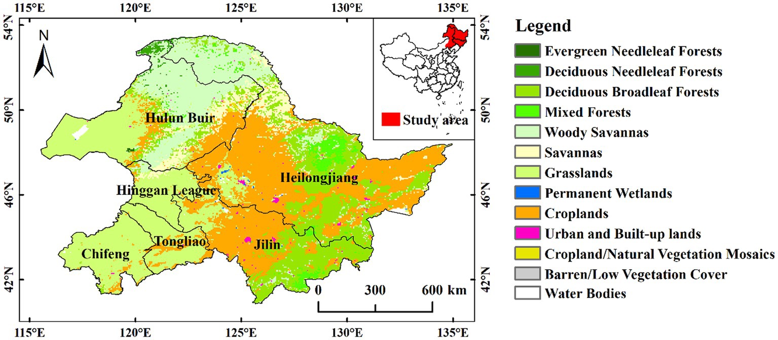
Figure 1. Map of vegetation cover types in the study area.

2.2. Datasets

In this study, various data products were used to explore the differences between vegetation greenness phenology and vegetation photosynthetic phenology. For consistency, the spatial resolution of these datasets was unified by mean method to 0.25° and time span from 2003 to 2018 in the analysis of the time lag between vegetation phenology and climatic factors.

2.2.1. Solar-induced chlorophyll fluorescence (SIF)

Contiguous SIF (CSIF) and global OCO-2 SIF (GOSIF) datasets were used to derive photosynthetic phenology. The CSIF dataset was generated using MODIS surface reflectance and a neural network approach (Zhang et al., 2018a).¹ CSIF dataset captures the seasonal and spatial changes of the original OCO-2 SIF in the far-infrared band (767 nm), which is shown to be closely related to the spatial and temporal variations of GPP (Zhang et al., 2016, 2018a; Sun et al., 2017). In this study, we used CSIF clear-daily from 2003 to 2019 with a temporal resolution of 4 days and spatial resolution of 0.05°. The CSIF clear sky product was chosen because of its strong correlation with the satellite retrieval SIF and also with GPP from the vorticity flux towers (Zhang et al., 2018a,b).

The GOSIF dataset with the continuous high spatial and temporal resolution was developed from discrete OCO-2 SIF, MODIS products, meteorological reanalysis data, and multiple regressions (Li and Xiao, 2019).² In this study, we used GOSIF from 2003 to 2019 with a temporal resolution of 8-day and spatial resolution of 0.05°. GOSIF had strong consistency (R² = 0.73, p < 0.001) with GPP from 91 FLUXNET2015 dataset (Li and Xiao, 2019).

2.2.2. MODIS products

Vegetation cover types were obtained from the MODIS MCD12C1 land cover type product of the International Geosphere-Biosphere Programme (IGBP) classification scheme. MODIS IGBP land cover type data are annual synthetic products with a spatial resolution of 0.05°. In addition, the 8-day synthetic surface spectral reflectance from MODIS MOD09A1 was used to calculate the EVI from 2003 to 2019. They are all available for free download at https://search.earthdata.nasa.gov/.

2.2.3. Climate data

Temperatures (Ts) were downloaded from the China Meteorological Forcing Dataset (CMFD, Yang and He, 2019; He et al., 2020)³ with a temporal resolution of days and a spatial resolution of 0.1°. In addition, soil moisture (SM) data were downloaded from the Global Land Evaporation Amsterdam Model (GLEAM) v3.5a (Miralles et al., 2011; Martens et al., 2017),⁴ with a temporal resolution of days and a spatial resolution of 0.25°.

2.3. Double logistic phenology method

We used a logistic function to fit the SIF and EVI observations (Zhang et al., 2003; Ganguly et al., 2010). To further eliminate the effect of outliers, the data were smoothed using Savitzky–Golay (SG) filtering (Chen et al., 2004). The logistic functional fitting method has advantages for estimating phenology with noisy data (Hird and Mcdermid, 2009). The fitting equation is (Zhang et al., 2003; Ganguly et al., 2010):

$\begin{array}{ll}VI\left(t\right)={\alpha }_1+\frac{{\alpha }_2}{1+\exp \left(-{\beta }_1\times \left(t-{\rho }_1\right)\right)}-\frac{{\alpha }_2}{1+\exp \left(-{\beta }_2\times \left(t-{\rho }_2\right)\right)}& (1)\end{array}$

where VI(t) denotes the SIF (or EVI) value at time t (days); ${\alpha }_1$is the value of the winter dormancy period; ${\alpha }_2$is the peak of the summer growth period; ${\beta }_1$ , ${\beta }_2$ , ${\rho }_1$ , and ${\rho }_2$ are parameters of this function to be estimated. The phenology indicators can be derived following (Gonsamo et al., 2017; Wang et al., 2019):

$\begin{array}{ll}SOS={\rho }_1-\frac{4.562}{2\times {\beta }_1}& (2)\end{array}$

$\begin{array}{ll}EOS={\rho }_2-\frac{4.562}{2\times {\beta }_2}& (3)\end{array}$

$\begin{array}{ll}\mathrm{GSL}=\mathrm{EOS}-\mathrm{SOS}& (4)\end{array}$

For consistency, hereinafter referred to as SOS, EOS, and GSL based on CSIF as SOS_CSIF, EOS_CSIF, and GSL_CSIF, respectively; and SOS, EOS, and GSL based on GOSIF as SOS_GOSIF, EOS_GOSIF, and GSL_GOSIF respectively; and SOS, EOS, and GSL based on EVI as SOS_EVI, EOS_EVI, and GSL_EVI, respectively.

2.4. Analysis

We analyzed the temporal and spatial patterns of phenology parameters for each dataset in the study area. We used multi-year means to represent the spatial patterns of SOS, EOS, and GSL and analyzed the rate of change of SOS, EOS, and GSL over time using the linear trend with the equation.

$\begin{array}{ll}Sl=\frac{n\times {{\displaystyle \sum }}_{y=1}^n\left(y\times Phe\left(i\mathrm{,}j\mathrm{,}y\right)\right)-\left({{\displaystyle \sum }}_{y=1}^{n}j\right)\times \left({{\displaystyle \sum }}_{y=1}^{n}Phe\left(i\mathrm{,}j\mathrm{,}y\right)\right)}{n\times \left({{\displaystyle \sum }}_{y=1}^n{y}^2\right)-{\left({{\displaystyle \sum }}_{y=1}^{n}y\right)}^2}& (5)\end{array}$

where y represents the year and takes values from 1 to n (n = 1,2, 3, …,17); Sl is the slope of the linear fit; Phe (i, j, y) represents the value of the pixel (i, j) in year y. Sl > 0 indicates that the value of the pixel is increasing, Sl < 0 indicates that the value of the pixel shows a decreasing trend. Moreover, the t-test was used to determine if Sl reached the 95% significance test.

Both SOS and EOS were strongly controlled by preseason climatic factors (Fu et al., 2015; Güsewell et al., 2017). To further understand the potential climate drivers of spatial and temporal patterns of phenology, we explored the correlations between phenological parameters and preseason climate factors using correlation and partial correlation analyses, extending forward in 5-day intervals from the SOS and EOS dates to the 200th day.

The date when climatic factors had the maximum absolute value of the correlation coefficient was defined as the preseason date when the phenological parameters were most correlated with climatic factors. The pixels that reached 95% significance were found according to correlation coefficient significance reference table. The partial correlation formula is:

$\begin{array}{ll}{R}_{\left(1\mathrm{,}2\mathrm{,}\mathrm{|}3\right)}=\frac{R_{12}-R_{13}\times R_{23}}{\sqrt{1-R_{13}^2}\times \sqrt{1-R_{23}^2}}& (6)\end{array}$

where $R_{12\left(3\right)}$ is the partial correlation coefficient between variable 1 and variable 2 after controlling for the linear effect of variable 3; $R_{12},$ $R_{13},$and $R_{23}$ are correlation coefficients between variable 1 and variable 2, variable 1 and variable 3, and variable 2 and variable 3, respectively.

3. Results

3.1. Temporal variation of photosynthetic and greenness phenology

From Figure 2, SOS_CSIF and SOS_EVI derived by DL from 2003 to 2019 showed advancement at the rate of-0.469 days/year (p < 0.01) and-0.324 days/year (p < 0.05), respectively, indicating that the rate of change of SOS_CSIF was greater than that of SOS_EVI over time. Then, EOS_CSIF and EOS_EVI derived using DL were delayed at the rates of 0.218 days/year (p < 0.05) and 0.023 days/year (p > 0.05), respectively over time, where the delay rate of EOS_CSIF was clearly higher than that of EOS_EVI. Finally, GSL_CSIF (0.675 days/year, p < 0.01) still lengthened at a greater rate than GSL_EVI (0.216 days/year, p > 0.05) over time. The change rates of SOS_CSIF, EOS_CSIF, and GSL_CSIF were more than the change rates of SOS_EVI, EOS_EVI, and GSL_EVI over time. Moreover, the rate of change of SOS_GOSIF, EOS_GOSIF, and GSL_GOSIF compared with SOS_EVI, EOS_EVI, and GSL_EVI was consistent with the findings of the rate of change of SOS_CSIF, EOS_CSIF, and GSL_CSIF compared with SOS_EVI, EOS_EVI, and GSL_EVI (Supplementary Figure S1). In summary, the rate of change in photosynthetic phenology (SOS, EOS, and GSL) derived from SIF over time was greater than the rate of change in greenness phenology (SOS, EOS, and GSL) derived from EVI over time.

FIGURE 2

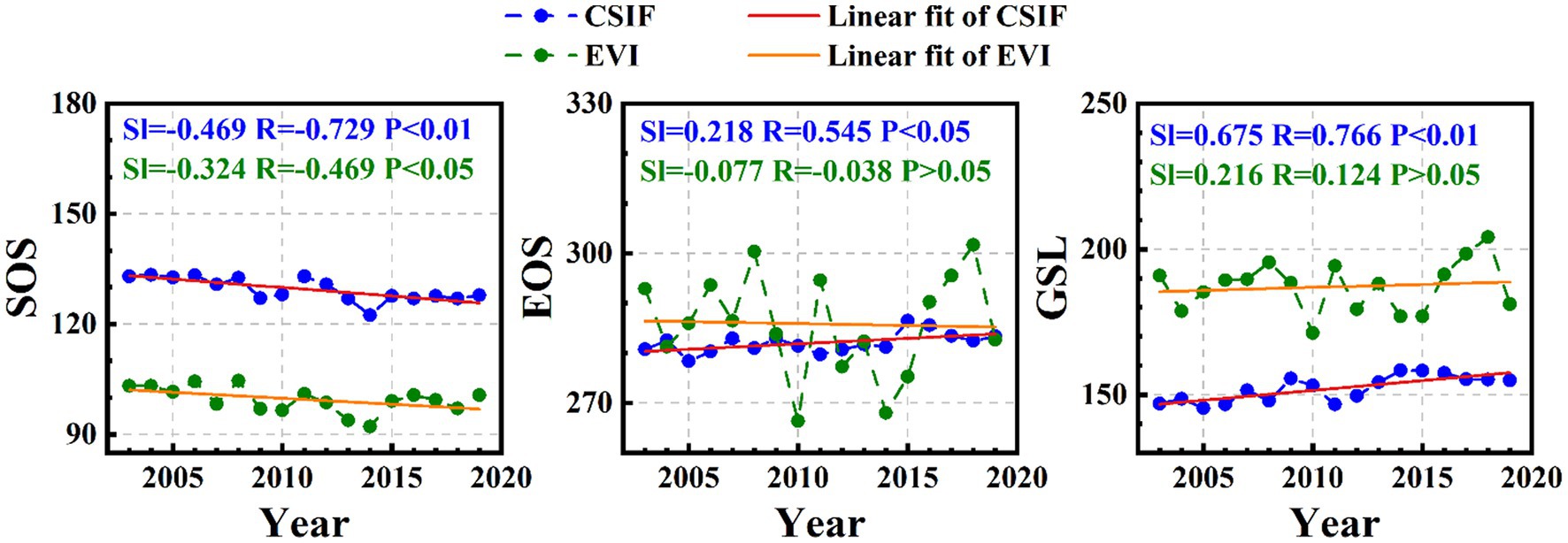
Figure 2. Trend of SOS, EOS, and GSL based on DL extraction of CSIF and EVI datasets.

3.2. Spatial variation of photosynthetic and greenness phenology

SOS_CSIF (or SOS_GOSIF) were dated from mid-April to May (Figure 3A and Supplementary Figure S2A), but SOS_EVI was dated from late March to mid-April (Figure 3D), with a clear spatial pattern in which the croplands were apparently later than the natural vegetation (Figures 1, 3A,D and Supplementary Figure S2A). Meanwhile, From Figure 3G and Supplementary Figure S2J, SOS_EVI was earlier than SOS_CSIF (or SOS_GOSIF), with mean values of 99.69, 122.68, and 130.31 days, respectively. EOS_CSIF (or EOS_GOSIF) and EOS_EVI showed an increasing trend from north to south (Figures 4B,E and Supplementary Figure S2B), but EOS_EVI (mean 283.26 days) was later than EOS_CSIF (mean 281.76 days) and EOS_GOSIF (281.48 days) (Figure 3H and Supplementary Figure S2H). The croplands’ SOS was later than natural vegetation and GSL_CSIF (or GSL_GOSIF) was also markedly shorter than natural vegetation for croplands (Figure 3C and Supplementary Figure S2C), but GSL_EVI did not perform clearly (Figure 3F). In terms of the length of GSL, from longest to shortest growing period were GSL_EVI (185.62 days), GSL_GOSIF (158.81 days), and GSL_CSIF (151.65 days) (Figure 3I and Supplementary Figure S2I). Overall, SOS_EVI spanned about 2 months. EOS_CSIF and EOS_GOSIF were shorter (about 1 month), but EOS_EVI spanned 2.5 months. GSL_CSIF and GSL_GOSIF had an 80-day spanned. GSL_EVI spanned 100 days. The results showed that the length of the greenness phenology growth period represented by EVI was greater than that characterized by SIF for photosynthetic phenology.

FIGURE 3

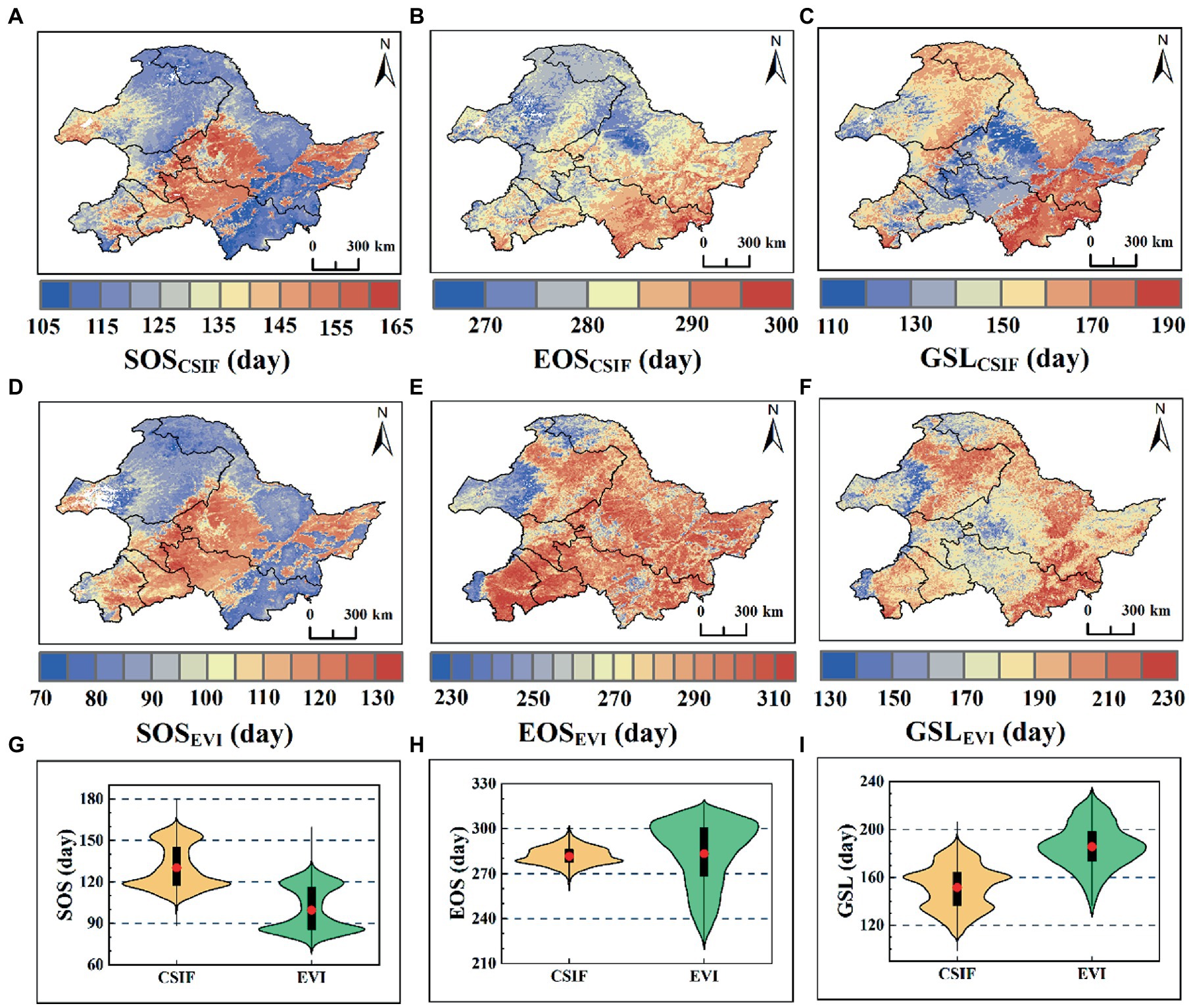
Figure 3. Spatial patterns of SOS, EOS and GSL means based on DL extracted CSIF and EVI datasets. (A–C) Spatial patterns of SOS, EOS, and GSL derived CSIF; (D–F) Spatial patterns of SOS, EOS, and GSL derived EVI; (G–I) Violin plots, where red dots indicate means, black rectangular boxes cover the interquartile range, and thin black lines reach the 5th and 95th percentiles.

FIGURE 4

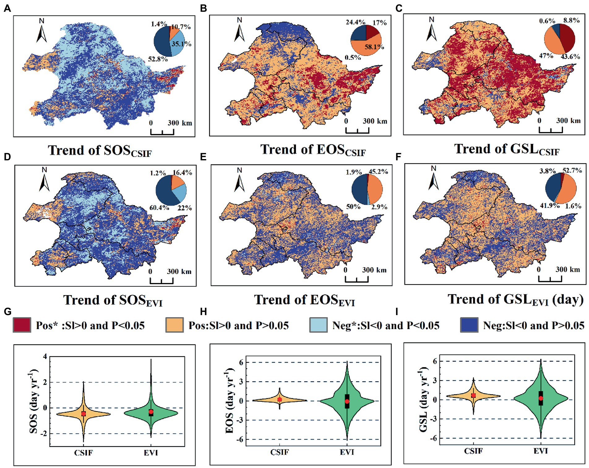
Figure 4. Spatial patterns of correlations between SOS and EOS extracted from CSIF and EVI and pre-season Ts, SM. (A–D) Spatial patterns of correlation coefficients between SOS, EOS derived CSIF and preseason Ts, SM; (E–H) Spatial patterns of correlation coefficients between SOS, EOS derived EVI and preseason Ts, SM; (I–L) Violin plots, where red dots indicate the mean, black rectangular boxes cover the interquartile range, and thin black lines reach the 5th and 95th percentiles. The black dot markers indicate that the 95% significance level was reached.

Next, we further analyzed the trends of SOS, EOS, and GSL pixels level derived from CSIF, GOSIF, and EVI, respectively, from 2003 to 2019. From Figure 5G and Supplementary Figure S3G, most areas of SOS_CSIF, SOS_GOSIF, and SOS_EVI showed an early trend, with 87.9, 89.2, and 82.4% of the areas advanced, respectively, of which 35.1, 44.4, and 22.0% of the pixels reached 95% significant level, respectively (Figures 5A,D and Supplementary Figure S3A). From Figure 5K and Supplementary Figure S3K, the areas of EOS_CSIF, EOS_GOSIF, and EOS_EVI delays varied widely, with 75.1, 67.8, and 47.0% of the pixels showing a delayed trend, respectively, and the percentage of those reaching the 95% significance level was also smaller, 17.0, 13.7, and 1.9%, respectively (Figures 5B,E and Supplementary Figure S3B). Comparison between SOS and EOS revealed that the area of SOS advancement and the percentage of reaching 95% significance were both obviously larger than the area of EOS delay and the percentage of reaching 95% significance. From Figure 5I and Supplementary Figure S3I, GSL_CSIF, GSL_GOSIF, and GSL_EVI showed a lengthened trend, with 90.6, 90.5, and 56.5% of the area showing a lengthened trend, respectively, of which 43.6, 43.7, and 3.8% of the pixels reached the 95% significance level (Figures 5C,F and Supplementary Figure S3C). The spatial variations of CSIF and GOSIF-derived phenological parameters were highly consistent, and the spatial trends between CSIF (or GOSIF) and EVI-extracted SOS were universally consistent. The results showed that the spatial patterns of photosynthetic phenology and greenness phenology differed to some extent, especially EOS and GSL.

FIGURE 5

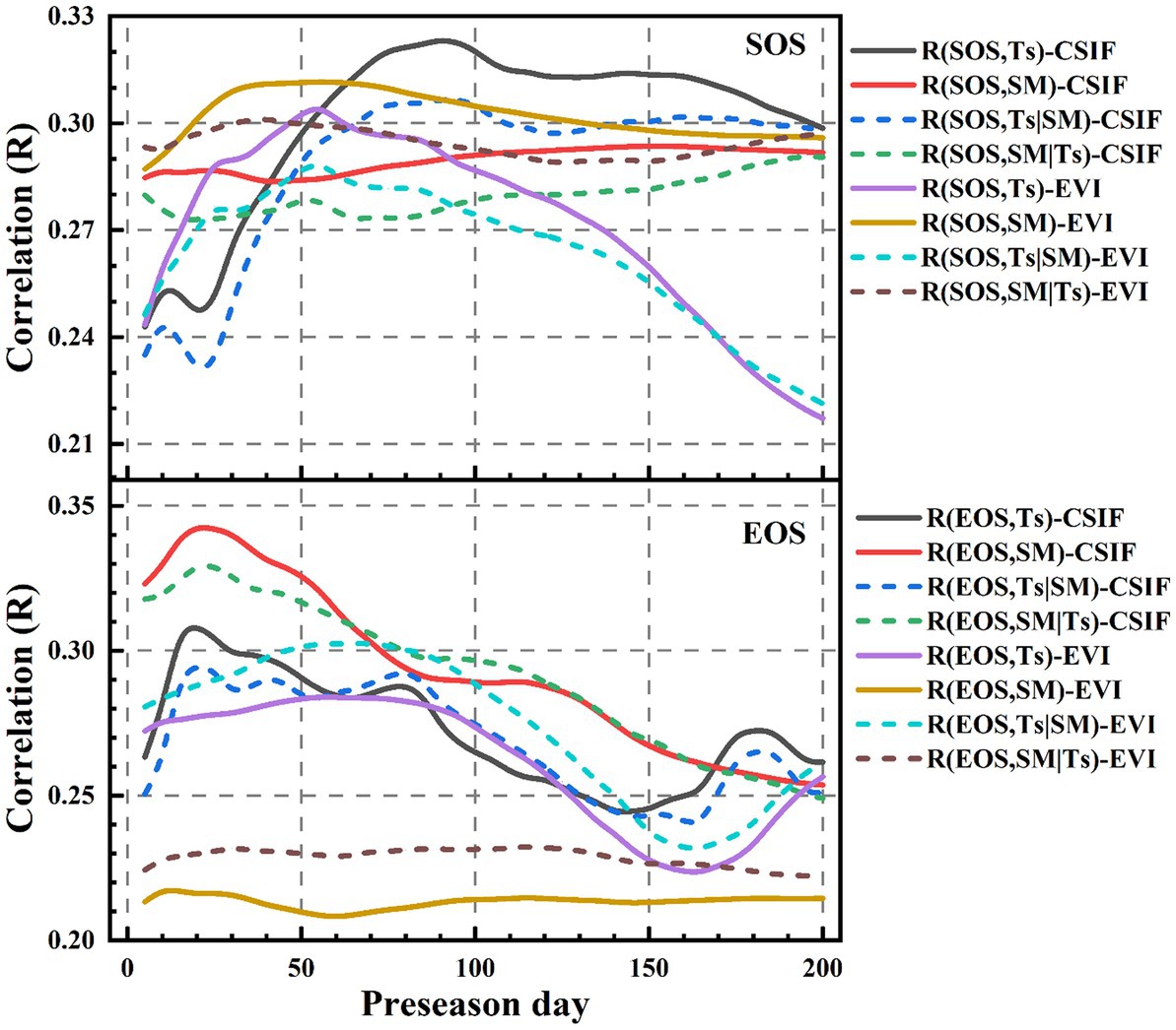
Figure 5. Spatial patterns of SOS, EOS, and GSL change rates and significance based on DL extracted CSIF and EVI datasets. (A–C) Spatial patterns of SOS, EOS, and GSL derived CSIF temporal rates of change and significance; (D–F), Spatial patterns of SOS, EOS, and GSL derived EVI temporal rates of change and significance; (G–I) Violin plots, where red dots indicate means, black rectangular boxes cover the interquartile range, and thin black lines reach the 5th and 95th percentiles.

3.3. Climatic determinants of photosynthetic and greenness phenology

Ts and SM are necessary for vegetation growth. Ts and SM affect vegetation photosynthesis under climate change (Zhang et al., 2010; Chong et al., 2017; Dang et al., 2022; Haerani et al., 2023; Zhao et al., 2023). Thus, the correlation and partial correlation analysis were used to explore the correlation between phenological parameters and preseason Ts and SM. From Figure 6, the correlation coefficients between SOS, EOS derived from CSIF, EVI, respectively, and preseason Ts, SM showed increasing then decreasing trends, respectively. Studies have shown that Ts and precipitation before the occurrence of phenology events play a key role in regulating phenology (Ge et al., 2015; Cao et al., 2018; Ren et al., 2019). This paper showed that the maximum correlation coefficients between SOS_EVI and preseason Ts were reached at the cumulative mean Ts of 2–3 months using correlation and partial correlation coefficients analysis (Figure 6), which was consistent with the existing study (Wu and Liu, 2013). But SOS_CSIF reached the maximum correlation about 1 month earlier than SOS_EVI (Figure 6). Compared to Ts, the correlation coefficients between SOS_CSIF and preseason SM (months 5–6) took longer to reach maximum correlation (Figure 6), which was consistent with previous finding (Piao et al., 2006). However, SOS_EVI was consistent with preseason SM and Ts. The maximum correlation coefficient was reached between EOS and preseason Ts, SM ranging from 20 to 60 days. And the timing of the maximum correlation coefficients between EOS_CSIF, EOS_EVI and preseason Ts, SM was generally consistent (Figure 6). In addition, SOS_GOSIF and EOS_GOSIF were consistent with the responses of SOS_CSIF and EOS_CSIF to preseason Ts and SM (Figure 6 and Supplementary Figure S4).

FIGURE 6

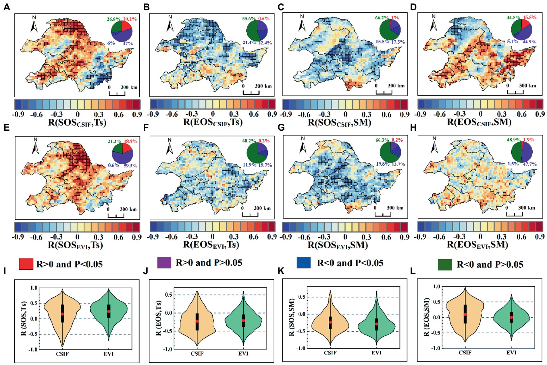
Figure 6. Correlation coefficients and partial correlation coefficients between CSIF, EVI derived SOS, EOS, respectively and pre-season Ts, SM over time.

We further analyzed the spatial distribution of correlation coefficients between SOS, EOS and preseason Ts, SM from the pixel level. From Figure 4I, SOS_CSIF and SOS_EVI were mostly positively correlated with Ts, with mean values of 0.153 and 0.237, respectively. The positive correlation coefficients between SOS_CSIF, SOS_EVI and Ts were 67.2 and 78.1% of the area, respectively, with positive correlation coefficients reaching 95% significance level accounting for 20.2 and 18.8% of the total number of pixels, respectively. The negative correlation coefficients between Ts and SOS_CSIF, SOS_EVI were mainly concentrated in the southeast of the pixels (Figures 4A,E). However, most areas of correlation coefficients between Ts and EOS_CSIF, EOS_EVI were negative with mean values of-0.229 and-0.209, respectively (Figure 4J). The area of negative correlation coefficients between EOS_CSIF, EOS_EVI and Ts were 77 and 80.1%, respectively, where the negative correlation coefficients reached 95% significance levels of 21.4 and 11.9% of the total number of pixels (Figures 4B,F). Compared to Ts, the correlations of SM with SOS and EOS were generally opposite, i.e., while SM was negatively correlated with SOS, SM was positively correlated with EOS (Figures 4K,L). The mean values of the correlation coefficients between SOS_CSIF, SOS_EVI and SM were −0.237 and −0.287, respectively, with the areas of negative correlation accounting for 81.7 and 86.1%, respectively, of which the areas reaching 95% significance level were 15.6 and 19.8%, respectively, and the areas reaching significance were mainly distributed in the middle (Figures 4C,G). The mean values of SM correlation coefficients with EOS_CSIF, and EOS_EVI were 0.1 and 0.0003, respectively (Figure 4L), with positive correlations of 60.4% (15.5% reaching 95% significance level) and 49.6% (1.9% reaching 95% significance level), respectively, concentrated in the southwest, upper center, and southeast. In addition, SOS_GOSIF, EOS_GOSIF and SOS_CSIF, EOS_CSIF responded consistently with pre-season Ts and SM at the pixel scale (Figure 4 and Supplementary Figure S5). The analysis at the pixel scale showed that the SM affected a larger area for SOS, but Ts affect a much larger area of EOS.

Next, we analyzed the spatial distribution between SOS, EOS and preseason Ts, SM using partial correlation (Figure 7). The overall partial correlation coefficients between preseason Ts and SOS_CSIF [59.9% (12.75% reaching 95% significance level)], SOS_EVI [74% (14.3% reaching 95% significance level)] were positive, where the mean values of the partial correlation coefficients were 0.081 and 0.197, respectively. The area of negative partial correlation between preseason Ts and SOS_CSIF, SOS_EVI were 40.1% (6.6% reaching 95% significance level) and 26% (0.6% reaching 95% significance level), respectively, concentrated in the southeast (Figures 7A,E,I). Compared to SOS, the partial correlations between preseason Ts and EOS_CSIF [75.1% (18.5% reaching 95% significance level)] and EOS_EVI [83% (12.3% reaching 95% significance level)] were overall negative, where the mean values of the partial correlation coefficients were −0.212 and −0.235 (Figures 7B,F,J). In addition, the partial correlations between preseason SM and SOS_CSIF, SOS_EVI were mostly negative. The mean values of the partial correlation coefficients between preseason SM and SOS_CSIF, SOS_EVI were −0.228 and −0.252, respectively, with the proportion of negative correlations for the pixels being 81.8% (13.2% reaching 95% significance level) and 82.2% (14.5% reaching 95% significance level), respectively (Figures 7C,G,K). However, the area of preseason SM positively correlated with EOS_CSIF and EOS_EVI were 58.5 and 47.6%, respectively, with 12.8 and 2.1% reaching the 95% significance level. Preseason SM was negatively correlated with EOS_CSIF and EOS_EVI with an area of 41.5% (5.8% reaching 95% significance level) and 52.4% (2% reaching 95% significance level), respectively. The area of positive and negative effects of preseason SM on EOS was approximately equal. The negative effects of preseason SM on EOS_CSIF were mainly concentrated in the north, but the negative effects on EOS_EVI were dispersed over the whole study area. Moreover, the partial correlation coefficients between preseason SM and EOS_CSIF (0.079) and EOS_EVI (−0.007) were around 0 (Figures 7D,H,L). Moreover, the partial correlation between SOS_GOSIF, EOS_GOSIF and SOS_EVI, EOS_EVI with pre-season Ts, SM compared with CSIF of phenology vs. EVI of phenology was highly consistent (Figure 7 and Supplementary Figure S6). Thus, the results indicated that the preseason SM affected SOS over a larger area, but EOS was more influenced by Ts.

FIGURE 7

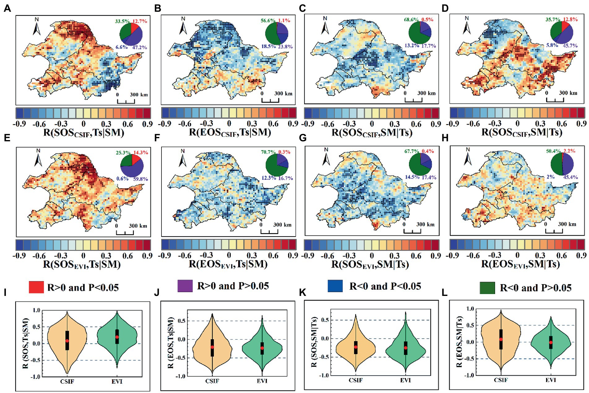
Figure 7. Spatial patterns of partial correlations between SOS and EOS extracted from CSIF and EVI and preseason Ts, SM. (A–D) Spatial patterns of partial correlation coefficients between SOS, EOS derived CSIF and preseason Ts, SM; (E–H) Spatial patterns of partial correlation coefficients between SOS, EOS derived EVI and preseason Ts, SM; (I–L) Violin plots, where red dots indicate the mean, black rectangular boxes cover the interquartile range, and thin black lines reach the 5th and 95th percentiles. The black dot markers indicate that the 95% significance level was reached.

4. Discussion

4.1. Comparison of photosynthesis and greenness phenology

Studies have found that there were systematic differences between photosynthetic and greenness phenology (Figures 2, 3). SOS_EVI was earlier than SOS_CSIF (or SOS_GOSIF), but EOS_EVI was later than EOS_CSIF (or EOS_GOSIF), resulting in greenness phenology growing approximately 20 days longer than photosynthetic phenology (Figure 3 and Supplementary Figure S2), which was consistent with the results of existing studies (Jeong et al., 2017; Meng et al., 2021). Moreover, the rate of change of photosynthetic phenology over time was 1.4–3.1 times greater than that of greenness phenology (Figure 2 and Supplementary Figure S1), which agreed with the results of existing work (Wang et al., 2019). The LUE model is available to explain the different performances in terms of EVI and SIF phenology (Walther et al., 2016; Yang et al., 2022). EVI is a robust proxy for fraction of absorbed photosynthetically active radiation (FAPAR) (Myneni and Williams, 1994) where not all photosynthetically active radiation (PAR) absorbed by the vegetation canopy is used for photosynthesis (Zhang et al., 2018c) but only light absorbed by chlorophyll is used for photosynthesis. The timing of photosynthesis in spring is later than the timing of growing leaves, which varies with leaf structure and longevity (Kikuzawa, 2003). Photosynthesis stops between chlorophyll reduction and leaf abscission due to light limitation (Daumard et al., 2010; Medvigy et al., 2013; Zhang et al., 2020). Also, there are differences in the phenology curves of SIF and EVI; both SIF and EVI are single-peaked curves, with the single peak of the SIF curve being steeper than that of EVI, and EVI decline in autumn slightly later than SIF resulting in a later autumn phenology extraction (Walther et al., 2016; Liu et al., 2018). In addition, SOS_CSIF (or SOS_GOSIF) was highly consistent with SOS_EVI in terms of spatial trends (Figures 3, 5 and Supplementary Figures S2, S3), however, EOS_CSIF (or EOS_GOSIF) was somewhat different from EOS_EVI in terms of spatial trends (Figures 3, 5 and Supplementary Figures S2, S3), which was consistent with the available findings (Meng et al., 2021). The FAPAR by chlorophyll is the dominant factor in spring photosynthetic phenology, while the total amount of photosynthetically active radiation absorbed by chlorophyll is the dominant factor in autumn when radiation determines photosynthetic phenology (Yang et al., 2022). Besides, autumn photosynthetic phenology is controlled by photoperiod, even if the leaves remain green (Bauerle et al., 2012). Therefore, there were some differences between the photosynthetic phenology of SIF and the greenness phenology of EVI using the same method of extraction.

4.2. Comparison of photosynthetic and greenness phenology in response to pre-season climatic determinants

We explored the spatial distribution of preseason Ts or SM with phenological parameters (SOS and EOS) using both correlation analysis and partial correlation analysis, and the results showed that the results of correlation analysis and partial correlation analysis were in high consistency (Figures 4, 7 and Supplementary Figures S5, S6). The spatial patterns of SOS_CSIF (or SOS_GOSIF), SOS_EVI with preseason Ts or SM showed high consistency, but the spatial patterns of EOS_CSIF (or EOS_GOSIF) with preseason Ts or SM were somewhat different from those of EOS_EVI with preseason Ts or SM. It may be related to the fact that SIF curves are more similar to NDVI in spring than in autumn (Jeong et al., 2017). In contrast to the greenness phenology information identified by EVI, SIF is mechanistically related to photosynthesis so it can rapidly respond to almost any factor that regulates photosynthetic activity (Porcar-Castell et al., 2014). This is because the photosynthetic phenology derived from SIF can also be constrained by environmental stress, as indicated by environmental factors in the LUE model (Monteith, 1972).

4.3. Limitations and outlook

This paper only considered the effects of Ts and SM on vegetation phenology. For vegetation phenology, radiation (Cong et al., 2017; Zhang et al., 2020), photoperiod (Basler and Korner, 2014), and accumulated temperature (Fu et al., 2013; Vitasse et al., 2017) may play more important roles. For example, the effect of radiation on photosynthetic phenology and greenness phenology varied considerably, especially at high latitudes in the Northern Hemisphere where photosynthetic phenology was affected by radiation limitation (Zhang et al., 2020). In addition, the study area included a larger crop area and anthropogenic influences on phenology were not considered. It is difficult to know how much each of the multiple influencing factors contributes, especially considering the coupling of solar radiation, human activities, and climatic environmental factors on vegetation phenology is difficult to distinguish their respective contributions. Third, the low spatial resolution of SIF used in this study is subject to scale effects (Liu et al., 2019; Shao et al., 2021), making it necessary to use high-resolution remote sensing data to derive vegetation phenology for the study. Finally, the impact of urban expansion (Zhuang et al., 2022a) and salinization (Zhuang et al., 2021, 2022b), which affect the photosynthesis of vegetation and cause changes in phenology, may also be considered. Therefore, future work will investigate the mechanisms and future predictions of climatic conditions on phenology evolution, the effects of urbanization and land use change on phenology and the combined effects of lag and scale effects on photosynthetic and greenness phenology.

5. Conclusion

In the study, DL was used to derive vegetation greenness and photosynthetic phenology to explore their spatial and temporal patterns and the relationship between pre-season climate determinants. The spatial and temporal variation of photosynthetic phenology extracted based on SIF and greenness phenology extracted by EVI were analyzed, and the results showed that there were systematic differences between photosynthetic and greenness phenology. The greenness phenology averages about 20 days longer than the photosynthetic phenology averages. Moreover, the rate of change of photosynthetic phenology over time was 1.4–3.1 times greater than that of greenness phenology. In addition, the results showed that photosynthetic phenology and greenness phenology were influenced by the same main factors. For spring greenness and photosynthetic phenology were highly consistent with pre-season Ts and SM, but for autumn greenness and photosynthetic phenology varied somewhat to pre-season Ts and SM. This study will help to better understand the differences between changes in vegetation greenness and photosynthetic phenology and their response to climatic factors, as well as to better employ vegetation phenology in the estimation of gross vegetation productivity.

Data availability statement

The original contributions presented in the study are included in the article/Supplementary material, further inquiries can be directed to the corresponding author.

Author contributions

CD conceived the idea and wrote the draft. ZS provided funding acquisition and supervision. XH revised the manuscript. QZ, GC, and JQ analyzed the data and validation. All authors contributed to the article and approved the submitted version.

Funding

This work was supported in part by the National Natural Science Foundation of China (Grant No. 42090012), the Guangxi Science and Technology Program (Grant No. 2021AB30019), 03 Special Research and 5G Project of Jiangxi Province in China (Grant No. 20212ABC03A09), Zhuhai Industry University Research Cooperation Project of China (Grant No. ZH22017001210098PWC), Sichuan Science and Technology Program (Grant Nos. 2022YFN0031, 2023YFS0381, and 2023YFN0022), Hubei Key R&D Plan (Grant No. 2022BAA048), and Zhizhuo Research Fund on Spatial–Temporal Artificial Intelligence (Grant No. ZZJJ202202).

Acknowledgments

The authors thank the reviewers for improving the manuscript with substantive and thoughtful comments and thank editor for feedback and assistance throughout.

Conflict of interest

The authors declare that the research was conducted in the absence of any commercial or financial relationships that could be construed as a potential conflict of interest.

Publisher’s note

All claims expressed in this article are solely those of the authors and do not necessarily represent those of their affiliated organizations, or those of the publisher, the editors and the reviewers. Any product that may be evaluated in this article, or claim that may be made by its manufacturer, is not guaranteed or endorsed by the publisher.

Supplementary material

The Supplementary material for this article can be found online at: https://www.frontiersin.org/articles/10.3389/ffgc.2023.1172220/full#supplementary-material

Footnotes

1. ^https://osf.io/8xqy6/

2. ^http://data.globalecology.unh.edu/data/GOSIF_v2/

3. ^http://data.tpdc.ac.cn/en/data/8028b944-daaa-4511-8769-965612652c49/

4. ^https://www.gleam.eu

References

Basler, D., and Korner, C. (2014). Photoperiod and temperature responses of bud swelling and bud burst in four temperate forest tree species. Tree Physiol. 34, 377–388. doi: 10.1093/treephys/tpu021

PubMed Abstract | CrossRef Full Text | Google Scholar

Bauerle, W. L., Oren, R., Way, D. A., Qian, S. S., Stoy, P. C., Thornton, P. E., et al. (2012). Photoperiodic regulation of the seasonal pattern of photosynthetic capacity and the implications for carbon cycling. Proc. Natl. Acad. Sci. U. S. A. 109, 8612–8617. doi: 10.1073/pnas.1119131109

PubMed Abstract | CrossRef Full Text | Google Scholar

Brown, M. E., and de Beurs, K. M. (2008). Evaluation of multi-sensor semi-arid crop season parameters based on NDVI and rainfall. Remote Sens. Environ. 112, 2261–2271. doi: 10.1016/j.rse.2007.10.008

CrossRef Full Text | Google Scholar

Buermann, W., Forkel, M., O’Sullivan, M., Sitch, S., Friedlingstein, P., Haverd, V., et al. (2018). Widespread seasonal compensation effects of spring warming on northern plant productivity. Nature 562, 110–114. doi: 10.1038/s41586-018-0555-7

CrossRef Full Text | Google Scholar

Cao, R. Y., Shen, M. G., Zhou, J., and Chen, J. (2018). Modeling vegetation green-up dates across the Tibetan plateau by including both seasonal and daily temperature and precipitation. Agric. For. Meteorol. 249, 176–186. doi: 10.1016/j.agrformet.2017.11.032

CrossRef Full Text | Google Scholar

Chang, Q., Xiao, X., Jiao, W., Wu, X., Doughty, R., Wang, J., et al. (2019). Assessing consistency of spring phenology of snow-covered forests as estimated by vegetation indices, gross primary production, and solar-induced chlorophyll fluorescence. Agric. For. Meteorol. 275, 305–316. doi: 10.1016/j.agrformet.2019.06.002

CrossRef Full Text | Google Scholar

Chen, J., Jönsson, P., Tamura, M., Gu, Z. H., Matsushita, B., and Eklundh, L. (2004). A simple method for reconstructing a high-quality NDVI time-series data set based on the Savitzky–Golay filter. Remote Sens. Environ. 91, 332–344. doi: 10.1016/j.rse.2004.03.014

CrossRef Full Text | Google Scholar

Chong, K. L., Kanniah, K. D., Pohl, C., and Tan, K. P. (2017). A review of remote sensing applications for oil palm studies. Geo. Spat. Inf. Sci 20, 184–200. doi: 10.1080/10095020.2017.1337317

CrossRef Full Text | Google Scholar

Cong, N., Shen, M. G., and Piao, S. L. (2017). Spatial variations in responses of vegetation autumn phenology to climate change on the Tibetan plateau. J. Plant Ecol. 10, 744–752. doi: 10.1093/jpe/rtw084

CrossRef Full Text | Google Scholar

Dang, C., Shao, Z., Huang, X., Qian, J., Cheng, G., Ding, Q., et al. (2022). Assessment of the importance of increasing temperature and decreasing soil moisture on global ecosystem productivity using solar-induced chlorophyll fluorescence. Glob. Chang. Biol. 28, 2066–2080. doi: 10.1111/gcb.16043

PubMed Abstract | CrossRef Full Text | Google Scholar

Daumard, F., Champagne, S., Fournier, A., Goulas, Y., Ounis, A., Hanocq, J.-F., et al. (2010). A field platform for continuous measurement of canopy fluorescence. IEEE Trans. Geosci. Remote 48, 3358–3368. doi: 10.1109/tgrs.2010.2046420

CrossRef Full Text | Google Scholar

dela Torre, D. M. G., Gao, J., and Macinnis-Ng, C. (2021b). Remote sensing-based estimation of rice yields using various models: A critical review. Geo. Spat. Inf. Sci 24, 580–603. doi: 10.1080/10095020.2021.1936656

CrossRef Full Text | Google Scholar

dela Torre, D. M. G., Gao, J., Macinnis-Ng, C., and Shi, Y. (2021a). Phenology-based delineation of irrigated and rain-fed paddy fields with Sentinel-2 imagery in Google earth engine. Geo. Spat. Inf. Sci 24, 695–710. doi: 10.1080/10095020.2021.1984183

CrossRef Full Text | Google Scholar

Frankenberg, C., Fisher, J. B., Worden, J., Badgley, G., Saatchi, S. S., Lee, J., et al. (2011). New global observations of the terrestrial carbon cycle from GOSAT: Patterns of plant fluorescence with gross primary productivity. Geophys. Res. Lett. 38:L17706. doi: 10.1029/2011gl048738

CrossRef Full Text | Google Scholar

Fu, Y. H., Campioli, M., Deckmyn, G., and Janssens, I. A. (2013). Sensitivity of leaf unfolding to experimental warming in three temperate tree species. Agric. For. Meteorol. 181, 125–132. doi: 10.1016/j.agrformet.2013.07.016

CrossRef Full Text | Google Scholar

Fu, Y. H., Zhao, H. F., Piao, S. L., Peaucelle, M., Peng, S. S., Zhou, G. Y., et al. (2015). Declining global warming effects on the phenology of spring leaf unfolding. Nature 526, 104–107. doi: 10.1038/nature15402

CrossRef Full Text | Google Scholar

Ganguly, S., Friedl, M. A., Tan, B., Zhang, X. Y., and Verma, M. (2010). Land surface phenology from MODIS: Characterization of the collection 5 global land cover dynamics product. Remote Sens. Environ. 114, 1805–1816. doi: 10.1016/j.rse.2010.04.005

CrossRef Full Text | Google Scholar

Ge, Q. S., Wang, H. J., Rutishauser, T., and Dai, J. H. (2015). Phenological response to climate change in China: A meta-analysis. Glob. Change Biol. 21, 265–274. doi: 10.1111/gcb.12648

CrossRef Full Text | Google Scholar

Gonsamo, A., Chen, J. M., and Ooi, Y. W. (2017). Peak season plant activity shif towards spring is refected by increasing carbon uptake by extratropical ecosystems. Glob. Change Biol. 24, 2117–2128. doi: 10.1111/gcb.14001

CrossRef Full Text | Google Scholar

Güsewell, S., Furrer, R., Gehrig, R., and Pietragalla, B. (2017). Changes in temperature sensitivity of spring phenology with recent climate warming in Switzerland are related to shifts of the preseason. Glob. Change Biol. 23, 5189–5202. doi: 10.1111/gcb.13781

PubMed Abstract | CrossRef Full Text | Google Scholar

Haerani, H., Apan, A., Nguyen-Huy, T., and Basnet, B. (2023). Modelling future spatial distribution of peanut crops in Australia under climate change scenarios. Geo. Spat. Inf. Sci. 1–20. doi: 10.1080/10095020.2022.2155255

CrossRef Full Text | Google Scholar

He, J., Yang, K., Tang, W. J., Lu, H., Qin, J., Chen, Y. Y., et al. (2020). The first high-resolution meteorological forcing dataset for land process studies over China. Sci. Data 7:25. doi: 10.1038/s41597-020-0369-y

PubMed Abstract | CrossRef Full Text | Google Scholar

Henebry, G. M., and de Beurs, K. M. (2013). “Remote sensing of land surface phenology: A prospectus” in Phenology: An Integrative Environmental Science. ed. M. D. Schwartz (Dordrecht: Springer Netherlands), 385–411.

Google Scholar

Hird, J. N., and Mcdermid, G. J. (2009). Noise reduction of ndvi time series: An empirical comparison of selected techniques. Remote Sens. Environ. 113, 248–258. doi: 10.1016/j.rse.2008.09.003

CrossRef Full Text | Google Scholar

Hufkens, K., Melaas, E. K., Mann, M. L., Foster, T., Ceballos, F., Robles, M., et al. (2019). Monitoring crop phenology using a smartphone based near-surface remote sensing approach. Agric. For. Meteorol. 265, 327–337. doi: 10.1016/j.agrformet.2018.11.002

CrossRef Full Text | Google Scholar

Jeong, S. J., Ho, C. H., Gim, H. J., and Brown, M. E. (2011). Phenology shifts at start vs. end of growing season in temperate vegetation over the northern hemisphere for the period 1982–2008. Glob. Change Biol. 17, 2385–2399. doi: 10.1111/j.1365-2486.2011.02397.x

CrossRef Full Text | Google Scholar

Jeong, S.-J., Schimel, D., Frankenberg, C., Drewry, D. T., Fisher, J. B., Verma, M., et al. (2017). Application of satellite solar-induced chlorophyll fluorescence to understanding large-scale variations in vegetation phenology and function over northern high latitude forests. Remote Sens. Environ. 190, 178–187. doi: 10.1016/j.rse.2016.11.021

CrossRef Full Text | Google Scholar

Jin, J. X., Wang, Y., Zhang, Z., Magliulo, V., Jiang, H., and Cheng, M. (2017). Phenology plays an important role in the regulation of terrestrial ecosystem water-use efficiency in the northern hemisphere. Remote Sens. 9:664. doi: 10.3390/rs9070664

CrossRef Full Text | Google Scholar

Keenan, T. F., Gray, J., Friedl, M. A., Toomey, M., Bohrer, G., Hollinger, D. Y., et al. (2014). Net carbon uptake has increased through warming-induced changes in temperate forest phenology. Nat. Clim. Chang. 4, 598–604. doi: 10.1038/nclimate2253

CrossRef Full Text | Google Scholar

Kikuzawa, K. (2003). Phenological and morphological adaptations to the light environment in two woody and two herbaceous plant species. Funct. Ecol. 17, 29–38. doi: 10.1046/j.1365-2435.2003.00707.x

CrossRef Full Text | Google Scholar

Li, M., Wang, X., and Chen, J. (2022). Assessment of grassland ecosystem services and analysis on its driving factors: A case study in Hulunbuir grassland. Front. Ecol. Evol. 10:25. doi: 10.3389/fevo.2022.841943

CrossRef Full Text | Google Scholar

Li, X., and Xiao, J. F. (2019). A global, 0.05-degree product of solar-induced chlorophyll fluorescence derived from OCO-2, MODIS, and reanalysis data. Remote Sens. 11:517. doi: 10.3390/rs11050517

CrossRef Full Text | Google Scholar

Li, X., Xiao, J. F., He, B. B., Arain, M. A., Beringer, J., Desai, A. R., et al. (2018). Solar-induced chlorophyll fluorescence is strongly correlated with terrestrial photosynthesis for a wide variety of biomes: First global analysis based on OCO-2 and flux tower observations. Glob. Change Biol. 24, 3990–4008. doi: 10.1111/gcb.14297

CrossRef Full Text | Google Scholar

Liu, Y., Dang, C., Yue, H., Lyu, C., and Dang, X. (2021). Enhanced drought detection and monitoring using sun-induced chlorophyll fluorescence over Hulun Buir grassland, China. Sci. Total Environ. 770:145271. doi: 10.1016/j.scitotenv.2021.145271

PubMed Abstract | CrossRef Full Text | Google Scholar

Liu, L. C., Shen, M., Chen, J., Wang, J., and Zhang, X. (2019). How does scale effect influence spring vegetation phenology estimated from satellite-derived vegetation indexes? Remote Sens. 11:2137. doi: 10.3390/rs11182137

CrossRef Full Text | Google Scholar

Liu, X. T., Zhou, L., Shi, H., Wang, S. Q., and Chi, Y. G. (2018). Phenological characteristics of temperate coniferous and broad-leaved mixed forests based on multiple remote sensing vegetation indices, chlorophyll fluorescence and CO2 flux data. Acta Ecol. Sin. 38, 3482–3494. doi: 10.5846/stxb20170821150

CrossRef Full Text | Google Scholar

Lobell, D. B., Burke, M. B., Tebaldi, C., Mastrandrea, M. D., Falcon, W. P., and Naylor, R. L. (2008). Prioritizing climate change adaptation needs for food security in 2030. Science 319, 607–610. doi: 10.1126/science.1152339

PubMed Abstract | CrossRef Full Text | Google Scholar

Mao, D. H., Wang, Z. M., Han, J. X., and Ren, C. Y. (2012). Spatio-temporal pattern of net primary productivity and its driven factors in Northeast China in 1982-2010. Sci. Geogr. Sin. 32, 1106–1111. doi: 10.13249/j.cnki.sgs.2012.09.1106

CrossRef Full Text | Google Scholar

Martens, B., Miralles, D. G., Lievens, H., van der Schalie, R., de Jeu, R. A. M., Fernández-Prieto, D., et al. (2017). GLEAM v3: Satellite-based land evaporation and root-zone soil moisture. Geosci. Model Dev. 10, 1903–1925. doi: 10.5194/gmd-10-1903-2017

CrossRef Full Text | Google Scholar

Medvigy, D., Jeong, S.-J., Clark, K. L., Skowronski, N. S., and Schäfer, K. V. R. (2013). Effects of seasonal variation of photosynthetic capacity on the carbon fluxes of a temperate deciduous forest. J. Geophys. Res. 118, 1703–1714. doi: 10.1002/2013jg002421

CrossRef Full Text | Google Scholar

Melaas, E. K., Friedl, M. A., and Richardson, A. D. (2016). Multiscale modeling of spring phenology across deciduous forests in the eastern United States. Glob. Change Biol. 22, 792–805. doi: 10.1111/gcb.13122

PubMed Abstract | CrossRef Full Text | Google Scholar

Meng, F. D., Huang, L., Chen, A. P., Zhang, Y., and Piao, S. L. (2021). Spring and autumn phenology across the Tibetan plateau inferred from normalized difference vegetation index and solar-induced chlorophyll fluorescence. Big Earth Data 5, 182–200. doi: 10.1080/20964471.2021.1920661

CrossRef Full Text | Google Scholar

Meroni, M., Rossini, M., Guanter, L., Alonso, L., Rascher, U., Colombo, R., et al. (2009). Remote sensing of solar-induced chlorophyll fluorescence: Review of methods and applications. Remote Sens. Environ. 113, 2037–2051. doi: 10.1016/j.rse.2009.05.003

CrossRef Full Text | Google Scholar

Miralles, D. G., Holmes, T. R. H., De Jeu, R. A. M., Gash, J. H., Meesters, A. G. C. A., and Dolman, A. J. (2011). Global land-surface evaporation estimated from satellite-based observations. Hydrol. Earth Syst. Sci. 15, 453–469. doi: 10.5194/hess-15-453-2011

CrossRef Full Text | Google Scholar

Monteith, J. L. (1972). Solar radiation and productivity in tropical ecosystems. J. Appl. Ecol. 9:747. doi: 10.2307/2401901

CrossRef Full Text | Google Scholar

Myneni, R. B., and Williams, D. L. (1994). On the relationship between FAPAR and NDVI. Remote Sens. Environ. 49, 200–211. doi: 10.1016/0034-4257(94)90016-7

CrossRef Full Text | Google Scholar

Piao, S. L., Ciais, P., Friedlingstein, P., Peylin, P., Reichstein, M., Luyssaert, S., et al. (2008). Net carbon dioxide losses of northern ecosystems in response to autumn warming. Nature 451, 49–52. doi: 10.1038/nature06444

PubMed Abstract | CrossRef Full Text | Google Scholar

Piao, S. L., Fang, J. Y., Zhou, L. M., Ciais, P., and Zhu, B. (2006). Variations in satellite-derived phenology in China’s temperate vegetation. Glob. Change Biol. 12, 672–685. doi: 10.1111/j.1365-2486.2006.01123.x

CrossRef Full Text | Google Scholar

Porcar-Castell, A., Tyystjärvi, E., Atherton, J., van der Tol, C., Flexas, J., Pfündel, E. E., et al. (2014). Linking chlorophyll a fluorescence to photosynthesis for remote sensing applications: Mechanisms and challenges. J. Exp. Bot. 65, 4065–4095. doi: 10.1093/jxb/eru191

CrossRef Full Text | Google Scholar

Ren, S. L., Qin, Q. M., Ren, H. Z., Sui, J., and Zhang, Y. (2019). New model for simulating autumn phenology of herbaceous plants in the inner Mongolian grassland. Agric. For. Meteorol. 275, 136–145. doi: 10.1016/j.agrformet.2019.05.011

CrossRef Full Text | Google Scholar

Richardson, A. D., Hufkens, K., Milliman, T., Aubrecht, D. M., Furze, M. E., Seyednasrollah, B., et al. (2018). Ecosystem warming extends vegetation activity but heightens vulnerability to cold temperatures. Nature 560, 368–371. doi: 10.1038/s41586-018-0399-1

PubMed Abstract | CrossRef Full Text | Google Scholar

Richardson, A. D., Keenan, T. F., Migliavacca, M., Ryu, Y., Sonnentag, O., and Toomey, M. (2013). Climate change, phenology, and phenological control of vegetation feedbacks to the climate system. Agric. For. Meteorol. 169, 156–173. doi: 10.1016/j.agrformet.2012.09.012

CrossRef Full Text | Google Scholar

Salas, E. A. L. (2020). Waveform LiDAR concepts and applications for potential vegetation phenology monitoring and modeling: A comprehensive review. Geo. Spat. Inf. Sci 24, 179–200. doi: 10.1080/10095020.2020.1761763

CrossRef Full Text | Google Scholar

Schwartz, M. D., Ahas, R., and Aasa, A. (2006). Onset of spring starting earlier across the northern hemisphere. Glob. Change Biol. 12, 343–351. doi: 10.1111/j.1365-2486.2005.01097.x

CrossRef Full Text | Google Scholar

Shao, Z., Wu, W., and Li, D. (2021). Spatio-temporal-spectral observation model for urban remote sensing. Geo. Spat. Inf. Sci. 24, 372–386. doi: 10.1080/10095020.2020.1864232

CrossRef Full Text | Google Scholar

Shen, M., Piao, S., Cong, N., Zhang, G., and Jassens, I. A. (2015). Precipitation impacts on vegetation spring phenology on the Tibetan plateau. Glob. Change Biol. 21, 3647–3656. doi: 10.1111/gcb.12961

PubMed Abstract | CrossRef Full Text | Google Scholar

Song, L., Guanter, L., Guan, K., You, L., Huete, A., Ju, W., et al. (2018). Satellite sun-induced chlorophyll fluorescence detects early response of winter wheat to heat stress in the Indian Indo-Gangetic Plains. Glob. Change Biol. 24, 4023–4037. doi: 10.1111/gcb.14302

PubMed Abstract | CrossRef Full Text | Google Scholar

Sun, Y., Frankenberg, C., Wood, J. D., Schimel, D. S., Jung, M., Guanter, L., et al. (2017). OCO-2 advances photosynthesis observation from space via solar-induced chlorophyll fluorescence. Science 358:5747. doi: 10.1126/science.aam5747

PubMed Abstract | CrossRef Full Text | Google Scholar

Tang, J., Körner, C., Muraoka, H., Piao, S., Shen, M., Thackeray, S. J., et al. (2016). Emerging opportunities and challenges in phenology: A review. Ecosphere 7:e01436. doi: 10.1002/ecs2.1436

CrossRef Full Text | Google Scholar

Vitasse, Y., Signarbieux, C., and Fu, Y. H. (2017). Global warming leads to more uniform spring phenology across elevations. Proc. Natl. Acad. Sci. U. S. A. 115, 1004–1008. doi: 10.1073/pnas.1717342115

PubMed Abstract | CrossRef Full Text | Google Scholar

Walther, S., Voigt, M., Thum, T., Gonsamo, A., Zhang, Y., Köhler, P., et al. (2016). Satellite chlorophyll fluorescence measurements reveal large-scale decoupling of photosynthesis and greenness dynamics in boreal evergreen forests. Glob. Change Biol. 22, 2979–2996. doi: 10.1111/gcb.13200

PubMed Abstract | CrossRef Full Text | Google Scholar

Wang, L., De Boeck, H. J., Chen, L., Song, C., Chen, Z., McNulty, S., et al. (2022). Urban warming increases the temperature sensitivity of spring vegetation phenology at 292 cities across China. Sci. Total Environ. 834:155154. doi: 10.1016/j.scitotenv.2022.155154

PubMed Abstract | CrossRef Full Text | Google Scholar

Wang, S. H., Ju, W. M., Peuelas, J., Cescatti, A., Zhou, Y., Fu, Y. Y., et al. (2019). Urban-rural gradients reveal joint control of elevated CO₂ and temperature on extended photosynthetic seasons. Nat. Ecol. Evol. 3, 1076–1085. doi: 10.1038/s41559-019-0931-1

PubMed Abstract | CrossRef Full Text | Google Scholar

Wang, Y., Xu, W., Yuan, W., Chen, X., Zhang, B., Fan, L., et al. (2021). Higher plant photosynthetic capability in autumn responding to low atmospheric vapor pressure deficit. Innovation 2:100163. doi: 10.1016/j.xinn.2021.100163

PubMed Abstract | CrossRef Full Text | Google Scholar

Westerling, A. L. (2006). Warming and earlier spring increase Western U.S. Forest wildfire activity. Science 313, 940–943. doi: 10.1126/science.1128834

PubMed Abstract | CrossRef Full Text | Google Scholar

White, M. A., Thornton, P. E., and Running, S. W. (1997). A continental phenology model for monitoring vegetation responses to interannual climatic variability. Global Biogeochem. Cy. 11, 217–234. doi: 10.1029/97gb00330

CrossRef Full Text | Google Scholar

Wu, X. C., and Liu, H. Y. (2013). Consistent shifts in spring vegetation green-up date across temperate biomes in China, 1982-2006. Glob. Change Biol. 19, 870–880. doi: 10.1111/gcb.12086

PubMed Abstract | CrossRef Full Text | Google Scholar

Xie, Q., Cleverly, J., Moore, C. E., Ding, Y., Hall, C. C., Ma, X., et al. (2022). Land surface phenology retrievals for arid and semi-arid ecosystems. ISPRS J. Photogramm. 185, 129–145. doi: 10.1016/j.isprsjprs.2022.01.017

CrossRef Full Text | Google Scholar

Yang, Y., Chen, R., Yin, G., Wang, C., Liu, G., Verger, A., et al. (2022). Divergent performances of vegetation indices in extracting photosynthetic phenology for northern deciduous broadleaf forests. IEEE Geosci. Remote Sens. Lett. 19, 1–5. doi: 10.1109/LGRS.2022.3182405

CrossRef Full Text | Google Scholar

Yang, K., and He, J. (2019). China meteorological forcing dataset (1979-2018). Beijing: National Tibetan Plateau Data Center.

Google Scholar

Yang, J., Zhang, X. C., Luo, Z. H., and Yu, X. J. (2017). Nonlinear variations of net primary productivity and its relationship with climate and vegetation phenology, China. Forests 8:361. doi: 10.3390/f8100361

CrossRef Full Text | Google Scholar

Yin, G., Verger, A., Filella, I., Descals, A., and Peñuelas, J. (2020). Divergent estimates of Forest photosynthetic phenology using structural and physiological vegetation indices. Geophys. Res. Lett. 47:e2020GL089167. doi: 10.1029/2020gl089167

CrossRef Full Text | Google Scholar

Yoshida, Y., Joiner, J., Tucker, C., Berry, J., Lee, J.-E., Walker, G., et al. (2015). The 2010 Russian drought impact on satellite measurements of solar-induced chlorophyll fluorescence: Insights from modeling and comparisons with parameters derived from satellite reflectances. Remote Sens. Environ. 166, 163–177. doi: 10.1016/j.rse.2015.06.008

CrossRef Full Text | Google Scholar

Zarco-Tejada, P. J., Morales, A., Testi, L., and Villalobos, F. J. (2013). Spatio-temporal patterns of chlorophyll fluorescence and physiological and structural indices acquired from hyperspectral imagery as compared with carbon fluxes measured with eddy covariance. Remote Sens. Environ. 133, 102–115. doi: 10.1016/j.rse.2013.02.003

CrossRef Full Text | Google Scholar

Zhang, L., Chen, X., Cai, X., and Salim, H. (2010). Spatial-temporal changes of NDVI and their relations with precipitation and temperature in Yangtze River basin from 1981 to 2001. Geo. Spat. Inf. Sci. 13, 186–190. doi: 10.1007/s11806-010-0339-1

CrossRef Full Text | Google Scholar

Zhang, Y., Commane, R., Zhou, S., Williams, A. P., and Gentine, P. (2020). Light limitation regulates the response of autumn terrestrial carbon uptake to warming. Nat. Clim. Chang. 10, 739–743. doi: 10.1038/s41558-020-0806-0

CrossRef Full Text | Google Scholar

Zhang, X. Y., Friedl, M. A., Schaaf, C. B., Strahler, A. H., Hodges, J. C. F., Gao, F., et al. (2003). Monitoring vegetation phenology using MODIS. Remote Sens. Environ. 84, 471–475. doi: 10.1016/s0034-4257(02)00135-9

CrossRef Full Text | Google Scholar

Zhang, Y., Joiner, J., Alemohammad, S. H., Zhou, S., and Gentine, P. (2018a). A global spatially contiguous solar-induced fluorescence (CSIF) dataset using neural networks. Biogeosciences 15, 5779–5800. doi: 10.5194/bg-15-5779-2018

CrossRef Full Text | Google Scholar

Zhang, Y., Xiao, X. M., Jin, C., Dong, J. W., Zhou, S., Wagle, P., et al. (2016). Consistency between sun-induced chlorophyll fluorescence and gross primary production of vegetation in North America. Remote Sens. Environ. 183, 154–169. doi: 10.1016/j.rse.2016.05.015

CrossRef Full Text | Google Scholar

Zhang, Y., Xiao, X., Wolf, S., Wu, J., Wu, X., Gioli, B., et al. (2018c). Spatio-temporal convergence of maximum daily light-use efficiency based on radiation absorption by canopy chlorophyll. Geophys. Res. Lett. 45, 3508–3519. doi: 10.1029/2017gl076354

CrossRef Full Text | Google Scholar

Zhang, Y., Xiao, X. M., Zhang, Y. G., Wolf, S., Zhou, S., Joiner, J., et al. (2018b). On the relationship between sub-daily instantaneous and daily total gross primary production: Implications for interpreting satellite-based SIF retrievals. Remote Sens. Environ. 205, 276–289. doi: 10.1016/j.rse.2017.12.009

CrossRef Full Text | Google Scholar

Zhao, F., Peng, Z., Qian, J., Chu, C., Zhao, Z., Chao, J., et al. (2023). Detection of geothermal potential based on land surface temperature derived from remotely sensed and in-situ data. Geo. Spat. Inf. Sci. 1–17. doi: 10.1080/10095020.2023.2178335

CrossRef Full Text | Google Scholar

Zhuang, Q., Shao, Z., Huang, X., Zhang, Y., Wu, W., Feng, X., et al. (2021). Evolution of soil salinization under the background of landscape patterns in the irrigated northern slopes of Tianshan Mountains, Xinjiang, China. Catena 206:105561. doi: 10.1016/j.catena.2021.105561

CrossRef Full Text | Google Scholar

Zhuang, Q., Shao, Z., Li, D., Huang, X., Altan, O., Wu, S., et al. (2022a). Isolating the direct and indirect impacts of urbanization on vegetation carbon sequestration capacity in a large oasis city: Evidence from Urumqi, China. Geo. Spat. Inf. Sci., 1–13. doi: 10.1080/10095020.2022.2118624

CrossRef Full Text | Google Scholar

Zhuang, Q., Shao, Z., Li, D., Huang, X., Cai, B., Altan, O., et al. (2022b). Unequal weakening of urbanization and soil salinization on vegetation production capacity. Geoderma 411:115712. doi: 10.1016/j.geoderma.2022.115712

CrossRef Full Text | Google Scholar