 Munkhnasan Lamchin
 Thomas Mumuni Bilintoh
 Woo-Kyun Lee
 Altansukh Ochir2
 Chul-Hee Lim
94% of researchers rate our articles as excellent or good
Learn more about the work of our research integrity team to safeguard the quality of each article we publish.
Find out more
ORIGINAL RESEARCH article
Front. For. Glob. Change, 11 October 2022
Sec. Forest Disturbance
Volume 5 - 2022 | https://doi.org/10.3389/ffgc.2022.994713
This article is part of the Research TopicGlobal Change in Forests and Their Communities: Analyzing Spatio-Temporal Changes in Forest Complex Socio-Ecological SystemsView all 4 articles
The rates of land degradation and urbanization has increased worldwide during the past century. Herein, we evaluate the spatio-temporal changes in global land cover via categorical intensity analysis of the European Space Agency’s climate change initiative (ESA-CCI) data for the period 1992 to 2018. Specifically, we evaluated intensity analysis at the category level for five time intervals, namely 1992–1997, 1997–2002, 2002–2007 and 2007–2012, 2012–2018. We also, evaluate the decrease and increase in the land cover at continental and climate zone. The study evaluates the following land cover categories: Cropland, Forest, SGO (Shrubland, Grassland, and Other), Urban, Bare areas, and WIS (Water, ice, and snow). After accuracy assessment, the global land-cover map for 2009 from the GlobCover data is selected, and a reclassified version of this map is used as a verification tool for comparison with the reclassified study data. The analysis of changes over the last 26 years shows that the loss for Cropland are dormant during the first and second time intervals, but active during the third, fourth, and fifth time intervals. By contrast, Forest experienced loss during all time intervals, and SGO experienced active loss only during the second time interval. Urban is the only category that experienced active gain during all time intervals. The present study also indicates that urbanization has and converted land in temperate regions during the past 26 years. Additionally, in South America and the tropical regions, the expansion of Cropland is the largest contributor to the decline in Forests and SGO.
Change in land cover can involve losses in the natural ecosystem, and can be triggered by human intervention through the use of various land cover types for different purposes (Mendoza-Ponce et al., 2018). Among the many drivers of change in land cover, anthropogenic and natural hazards are key factors. Land cover changes contribute to global environmental change (Shrestha et al., 2018). Hence, scientists and decision-makers are increasingly using change analysis to study the changes in the global environment (Foley et al., 2005). In this respect, land-use and land-cover change (LULCC) is an essential variable of change globally, and is mostly affected by regional changes, which, in turn, mainly concern environmental changes (Mendoza-Ponce et al., 2018; Lamchin et al., 2020). Although this is usually a phase of several decades in length, it is greatly accelerated by human forces such as urbanization and industrial agriculture, and natural phenomena such as flooding or rising sea levels (Foley et al., 2005; Ghimire et al., 2014; Shrestha et al., 2018). The LULCC is essentially equivalent to the perturbation of natural ecosystems by man (Klein Goldewijk, 2016), and is a major cause of climate change and global and regional environmental change (Foley et al., 2005; Bonan, 2008; Brovkin et al., 2013; Alkama and Cescatti, 2016).
Pontius et al. (2013) developed a thorough understanding of land cover and land use analysis concerning change intensity, where the intensity assesses the land use changes by evaluating stability (Sang et al., 2019). To quantify intensity, researchers have proposed sophisticated methods such as intensity analysis (Fang et al., 2018; Quan et al., 2019; Sang et al., 2019; Shafizadeh-Moghadam et al., 2019; Feng et al., 2020), and advanced statistical methods have been developed to evaluate the modeling results and explain the potential motives for land-use change (Aldwaik and Pontius, 2012; Pontius et al., 2013). During the last decade, advancements in quantity analysis, spatial mapping, and satellite-based monitoring have been employed to assess land-use change (Olmedo et al., 2015; Pickard et al., 2017; van Vliet, 2019; Liu et al., 2020). These studies help identify the factors that might affect land-cover changes, and how humans affect land-cover changes and the environment (Wang et al., 2012; Cloern et al., 2016; Fang et al., 2018). Thus, several studies have used historical land-cover change analysis to reveal how humans have impacted the natural environment (Klein Goldewijk et al., 2011), while others have used GIS modeling tools to investigate the global effect of land-cover transition (Veldkamp and Verburg, 2004; Liu and Tian, 2010; Jepsen et al., 2015). For example, the LULC model has been used to analyze land-cover change and generate predictions for the identification of trends in the LUCC (Václavík and Rogan, 2009), urban growth, deforestation in the tropics (Khoi and Murayama, 2010), modeling of habitat (Gontier et al., 2010), Muzaffarpur in India (Mishra et al., 2014), and erosion concerning conservation (Gaspari et al., 2009). In addition, remote-sensing, GIS, and LULC modeling have been used to study land use in Kashmir, India (Amin and Fazal, 2012), while a Land Transition Agent-Based Model (LTABM) has been applied to a case study on the land transition in the Missisquoi, Canada watershed (Amin and Fazal, 2012; Tsai et al., 2013; Pandolfi, 2016).
In the present study, we employ remotely sensed data and geospatial techniques to analyze spatio-temporal changes in global land cover during 6-year time intervals. Categorical intensity analysis of global temporal differences in the European Space Agency’s climate change initiative (ESA-CCI) dataset indicates significant change during the past 26 years. This has resulted in the identification of distinct land cover dynamics within and between the Earth’s continents and climate zones. In detail, we compute the total area gained and lost by each land cover type and map the evolution of the magnitude of the transition between land cover types. The specific goals of the study were as follows:
1. To evaluate the categorical intensity analysis and determine the extent to which each deviation from the starting value of each category differs from a uniform intensity around the world.
2. To assess the change in gain intensity of each category, expressed as a percentage of the end size derived from global adjustments over an interval. Quan et al. (2019) defines a category’s gain intensity as the percentage of the category’s end size that derives from the gain during the time interval, whiles a category’s loss intensity is percentage of the start size of category that loses during the time interval. As a result, we make reference to these definitions whenever we use the phrases “gain intensity” and “loss intensity.”
3. To evaluate how the land cover has changed over the long-term at the global level and within climatic zones on a continental scale.
The newly released annual ESA-CCI land-cover (LC) maps provide continuous information about land-cover changes at 300 m resolution for the period from 1992 to 2018. The full data archive of the medium resolution imaging spectrometer (MERIS) satellite from 2003 to 2012 provides 15 spectral bands at 300 m resolution. A baseline was established for this dataset by combining the outputs of machine learning and unsupervised algorithms (ESA, 2017). Recordings of time series at 1 × 1 km spatial resolution were conducted between 1992 and 1999 by the Advanced Very High Resolution Radiometer (AVHRR) satellite, between 1999 and 2013 by the Satellite SPOT-VGT, and between 2014 and 2015 by the Project for On-Board Autonomy – Vegetation (PROBA-V) satellite. Data collected from these recordings were used to detect and confirm changes in land cover. After 2004, when possible, these changes were delineated at a 300-m spatial resolution. The 10-year delineating process produced 24 annual land change (LC) maps spanning the period from 1992 to 2015. A vital component of the classification process required that each change persisted for a time period greater than 2 consecutive years. Further details can be found in the ESA-CCI-LC Product User Guide (ESA, 2017). The classification process yielded a collection of annual LC maps from 1992 to 2018, with a spatial resolution of 300 m. The classification algorithm used pixel-based uncertainty to report the level of confidence for each pixel’s LC classification, and evaluated the LC products using an accepted international standard. This evaluation procedure derived accuracy from a confusion matrix. In addition, a panel of international experts built an object-based validation database comprised of 2,600 primary sampling units in order to assess the accuracy of the LC classes and changes (ESA, 2017).1 Further validation was performed by the present authors by using GlobCover data 2009.2
In the ESA-CCI data, the surface of the Earth is divided into 37 initial LC classes using the United Nations Land-Cover Classification System -UN-LCCS (Di Gregorio, 2005). Hence, each pixel in the land-cover image is assigned a class between 1 and 37. In the present study, the results for 1992, 1997, 2002, 2007, 2012, 2015, and 2018 were re-classified into six classes based on the IPCC land categories used by ESA (2017), as shown in Table 1. To reclassify the land-cover image in GRASS3, a new mapset was built, and each class was allocated and integrated based on an understanding and interpretation of the LC class definitions. The reclassified land-cover maps are presented in Figure 1, along with the breakdown by percentage of each category as a pie chart.
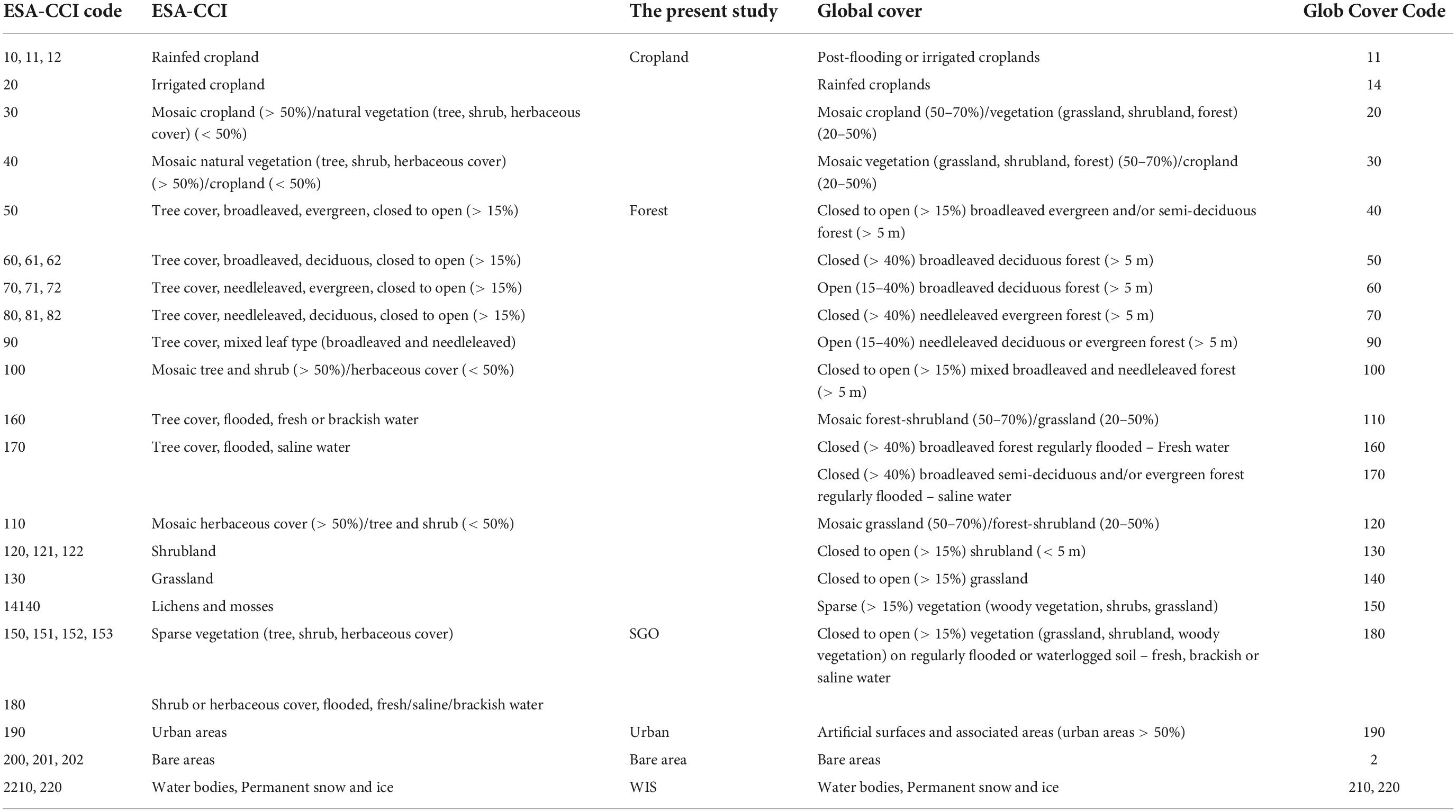
Table 1. The land-cover (LC) classes of the ESA, GlobCover, and the present study.
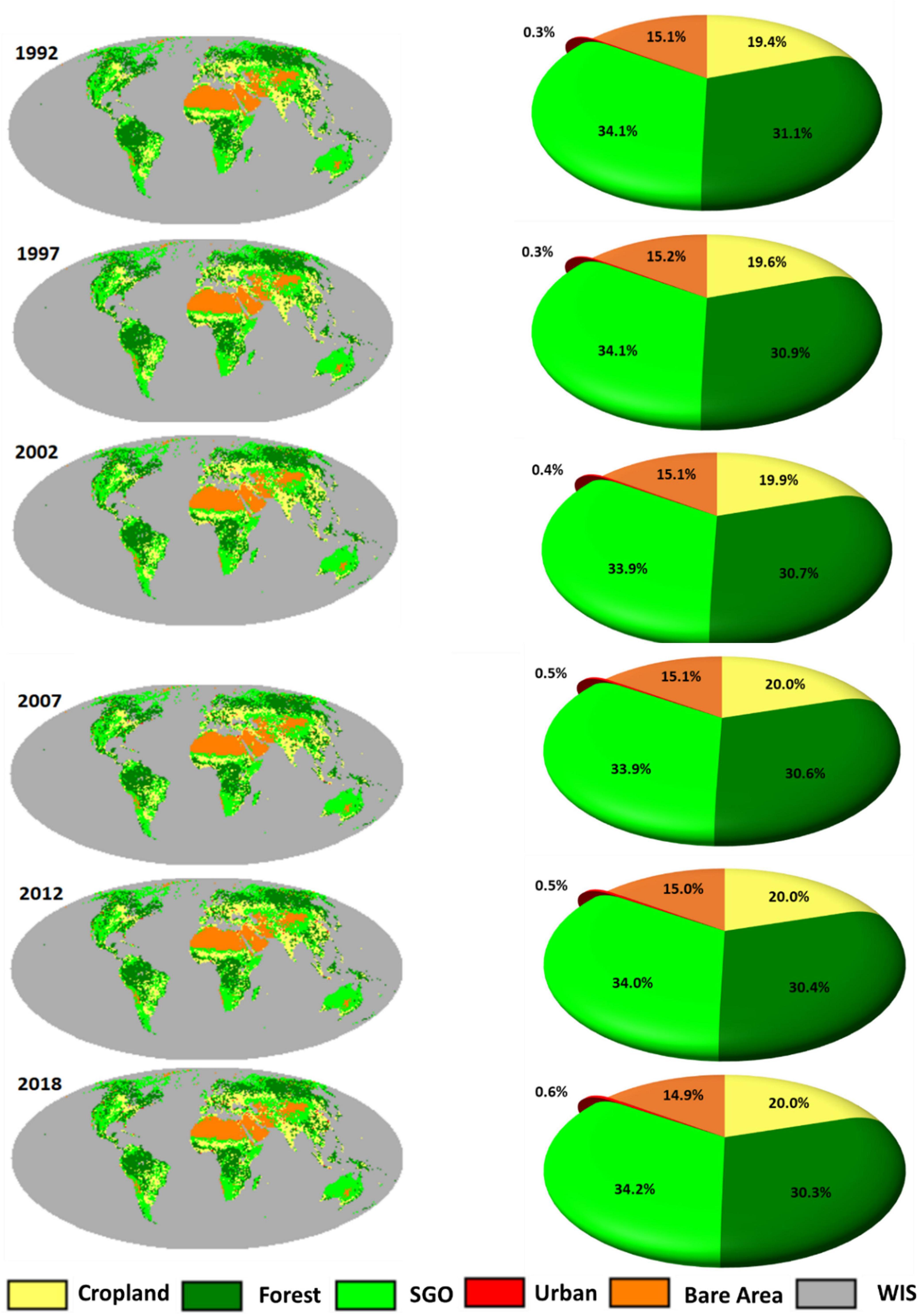
Figure 1. Spatial distribution of land-cover classes on maps for 1992, 1997, 2002, 2007, 2012, and 2018 (left) and the corresponding pie charts showing the breakdown percentage of each category (right).
Although there are variants of each class in the Olivier et al. (2010) map that are comparable to the LULC classes in the ESA-CCI, these variants are not identical. Hence, the same procedure was used to reclassify the 22 classes that make up the 2009 GlobCover map into six classes for the present study. The input data for the ESA-CCI is a multi-facet of sensors such as SAR and Landsat. Obviously, these sensors have different radiometric sensitivities, which users must note. ESA-CCI addresses this problem by applying a spatially and temporally weighted regression (STWR) model to the images derived from the sensors (ESA, 2020). As a result, ESA-CCI normalizes the effect of the difference in the radiometric properties of the sensors. ESA-CCI applies a similar method to account for the geometric variations in the images derived from the different sensors.4
For verification of the sampling accuracy on a global scale, the Google earth engine used an equal sample of points for all classes using the GlobCover map as the reference data. For this procedure, the resolution of the GlobCover map was reduced, and each pixel was converted into an individual point. In total, 148,793 points were extracted and used as sampling points for the verification process. The values of the reclassified GlobCover and ESA-CCI map data corresponding to the 148,793 sample points were then extracted, and the accuracy of the ESA-CCI map was verified by using a confusion matrix containing the class values of each map corresponding to the verification sample point. This was followed by calculation of the producer accuracy, user accuracy, and overall accuracy. Patel and Kaushal (2010) provides definitions and details of the three types of accuracies.
We examined intensity analysis at the category level for a total of five different time intervals, namely 1992–1997, 1997–2002, 2002–2007, 2007–2012, and 2012–2018. Intensity analysis is a quantitative tool used to study land use at a categorical, interval, and transitional level (Aldwaik and Pontius, 2012; Teixeira et al., 2016). The interval intensities measure the variations in both the size and the annual rate of change during each specific time interval. A time interval is the amount of time that passes between two different time points. As a result, the intensity of the intervals provides information about which sites experience a slow or rapid annual rate of change (Table 2). The magnitudes of each category’s gross gains and losses are measured by the categorical level intensity metric, which sheds light on which categories are inactive or active during a specified period of time. Consequently, categorical level intensity analysis indicates which patterns of change are consistent across the specified time intervals. Meanwhile, the transitional level intensity metric indicates which category’s transitions are being intensified or little affected during the specified time period. This present study focuses on categorical level intensity analysis.
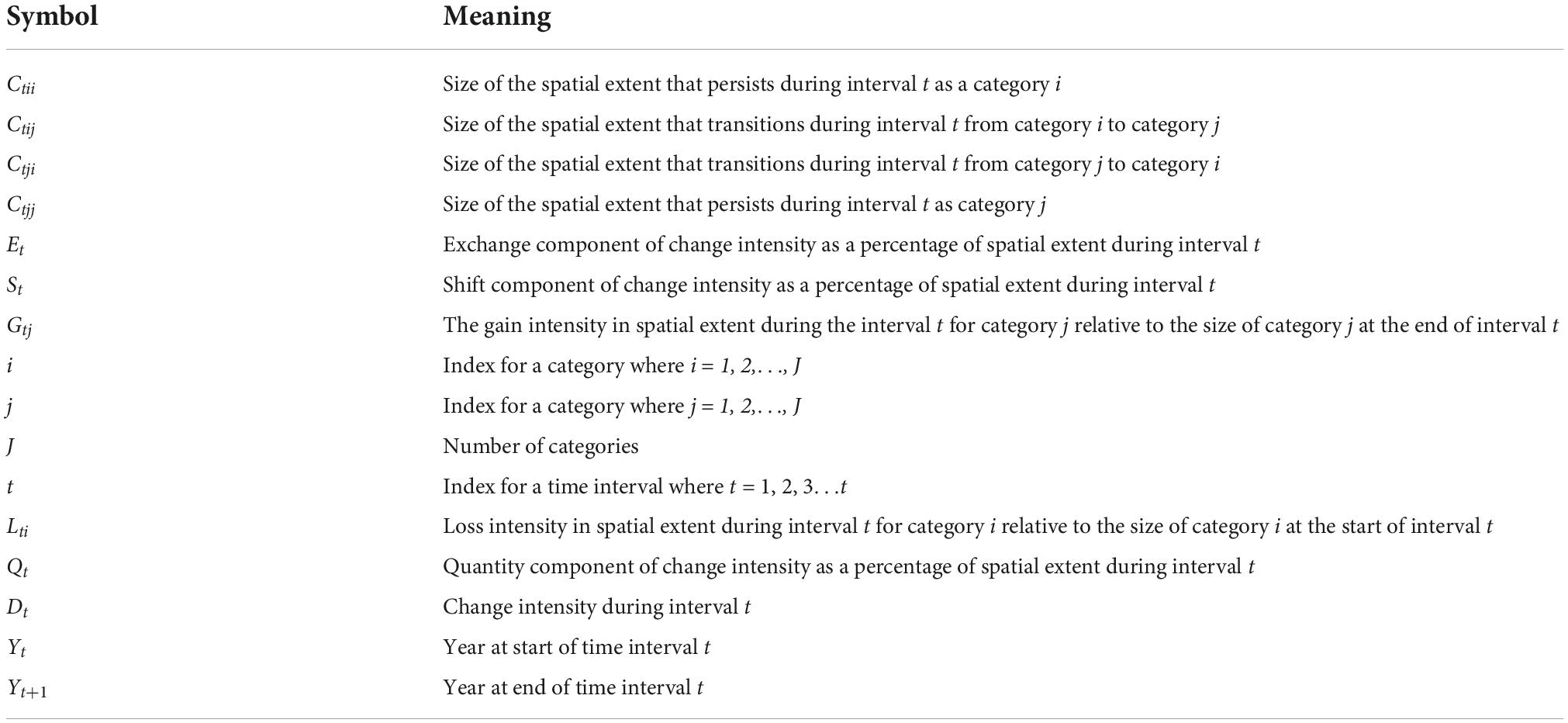
Table 2. Mathematical notations of the categorical intensity analysis.
First, we compute the three components of change: Quantity, Exchange, and Shift using Eqs. 1–4. Equation 2 is divided by 2 because each change involves a loss and gain category (Chen and Gilmore Pontius, 2011). Next, we use Eqs. 5–8 to compute the intensities of Gross Change, Quantity, Exchange, and Shift. This approach allows us to show the intensities of the components of change in Figures 2B,D,F,H,J. Finally, Eqs. 9, 10 compute each category’s loss and gain intensity, which we compare to the uniform intensity Dt, which is the bar called “Extent” in Figure 2.
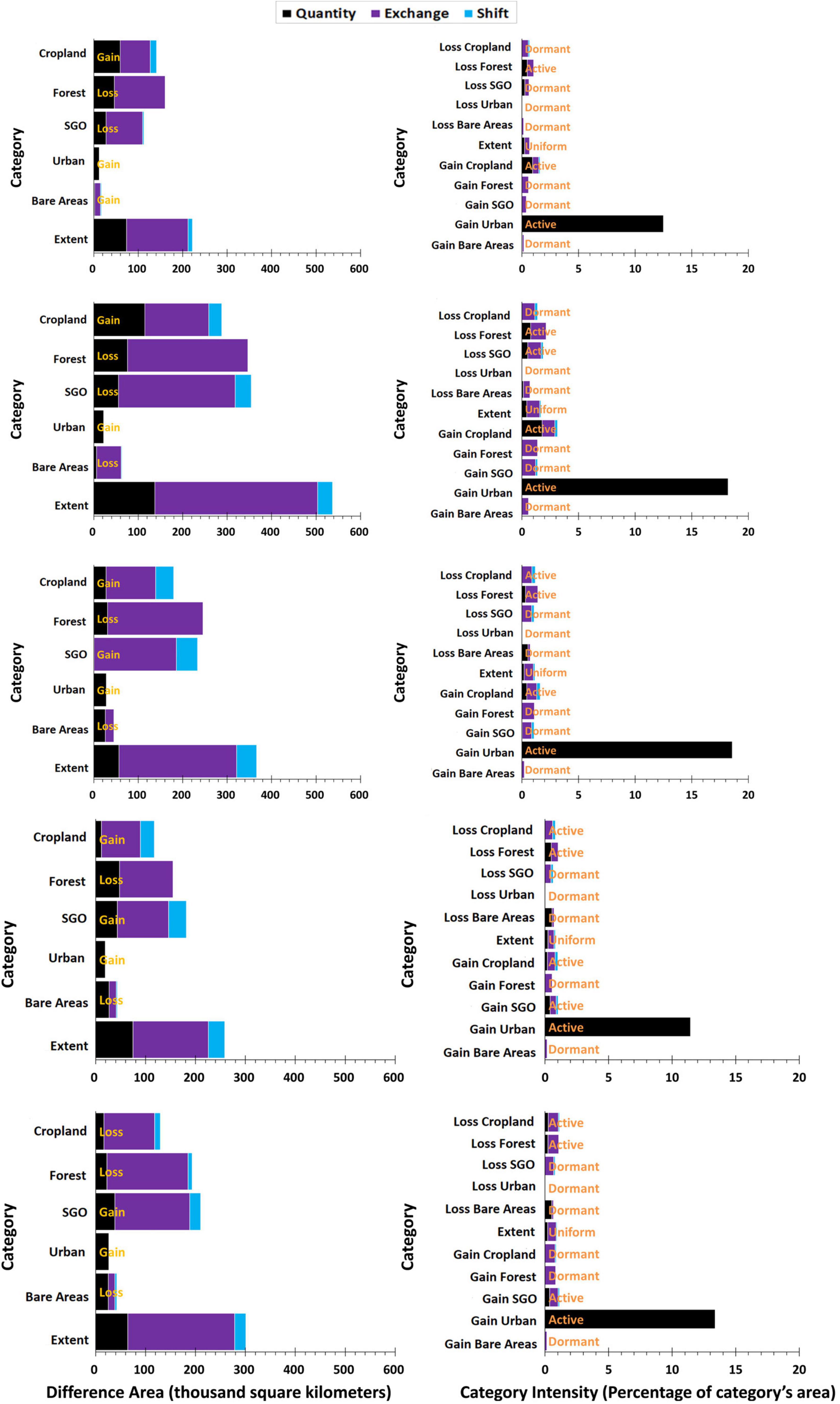
Figure 2. The categorical level losses and gains in terms of the difference areas (left-hand side) and intensities (right-hand side) during the time intervals 1992–1997, 1997–2002, 2002–2007 and 2007–2012, 2012–2018. The intensities for each category are divided into the three components of change: Quantity (black), Exchange (purple), and Shift (blue).
Lti computes the size of the loss intensity of a category (i) as the percentage of the category’s start size that is lost during the time interval Yt + 1−Yt Similarly, Gtj computes the size of a category’s (j) gain intensity as the percentage of the end size of the category that is gained during time interval Yt + 1−Yt. Thus, comparing Dt to Lti and Gtj reveals which category’s losses and gains are active or dormant. Specifically, if Lti < Dtior Gtj < Dti then loss and gain of categories i and j is dormant. If Lti > Dti or Gtj > Dti, then loss and gain of categories i and j is active. Finally, if Lti = Dti or Gtj = Dti then loss and gain of categories i and j is uniform. We modified the equations after Bilintoh (2022).
The user’s and producer’s accuracies for the various land cover types in the ESA-CCI and GlobCover maps are compared in Table 3. Here, the WIS category is assessed with a high accuracy of > 90%, the Bare area and Forest categories are calculated with moderate accuracies of 70–90%, but Cropland, SGO, and urban classes are evaluated with low accuracies of < 65%. Thus, the sample-point based accuracy analysis for the two reclassified maps indicates an overall accuracy of 92%, with a Kappa coefficient of 0.82.
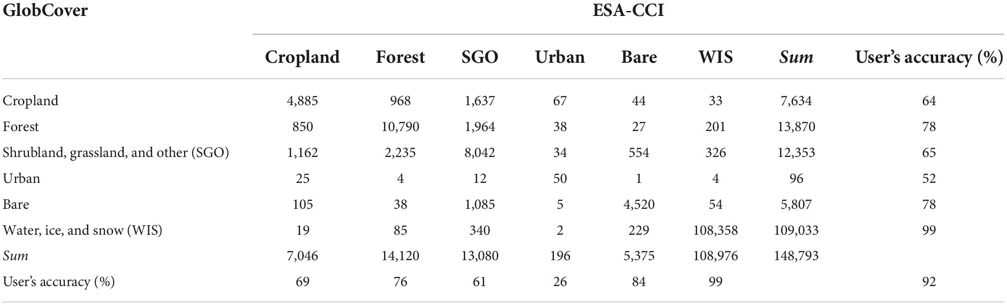
Table 3. The confusion matrix of the ESA-CCI and GlobCover maps for 2009.
The categorical level losses and gains (in thousands of square kilometers and area percentage) are indicated in in terms of both the difference area (left-hand side) and intensity (right-hand side) during the time intervals 1992–1997, 1997–2002, 2002–2007, 2007–2012, and 2012–2018. In the left-hand plots, the individual components of Quantity, Exchange, and Shift for each category are indicated by the black, purple, and blue areas, respectively. The area for each component of change was derived from Eqs. 1–4. Here, Cropland shows net gain only during the first, second, third, and fourth time intervals, Forest shows net loss during all time intervals, SGO shows net loss during the first three time intervals and net gain during the last two time intervals, Urban experiences net gain during all time intervals, and Bare areas show a net gain during the first time interval and net loss during the second, third, fourth, and fifth time intervals. Moreover, the right-hand side of Figure 2 indicates that the changes in Cropland and SGO involve all three components (i.e., Quantity, Exchange, and Shift) during all time intervals, whereas the change in Urban areas consists only of Quantity during all time intervals.
Additionally, the right-hand plots in Figure 2 provide information concerning each category’s gross loss or gain for each time interval. Here, the size of the losses and gains for every category are in units of percentage of area, thus indicating whether a category’s change is positive, negative, or zero. To gain further insights, the present study focuses on those categories with the biggest losses and gains.
In the left-hand plots of Figure 2, the Extent bars indicate whether the intensities of change are uniform, active, or dormant. If a category’s intensity falls short of the extent bar, then the category’s temporal difference is dormant. If a category’s intensity extends beyond the Extent bar, then the category’s temporal difference is active. If a category’s intensity equals the Extent bar, then the category’s temporal difference is uniform. Thus, the loss intensity for Cropland is dormant during the first and second time intervals, but active during the third, fourth, and last time intervals. Forest experiences active loss intensities during all time intervals. SGO experiences active loss only during the second time interval, with dormant loss intensities during all other time intervals. Urban is the only category that experiences active gain intensities during all time intervals.
The previous section used categorical level intensity analysis to examine the size and proportions of each category’s change. The present section examines the global land cover changes and exchanges during the temporal extent. Here, the global land cover area during 1992–2018 is seen to be variable, changing by a total of 6981654.3 km2 representing 5.18% of the global area. The largest non-persistent change in Forest is 2,619,453 km2, representing 6.5% of the global forest area during the entire temporal extent. Most of this occurred through losses in the Amazon, Savanna, South-east Asia, North America, Russia (Siberia), western Europe, and northeast Asia. The largest change in Cropland is 1,253,213 km2 about 5% of the total cropland of the world over the entire temporal extent. Again, this was mainly in the Amazon, with some areas in northern America, Africa, central Asia, the Korean Peninsula, northeastern China, and southeastern China. Major changes are observed in the SGO cover, which changed by 5.4% in Alaska, the western part of North America, the Amazon, Savanna areas, the eastern and western parts of Australia, and southeastern Asia over the 26-year period. Meanwhile, Urban areas increased by 0.09% overall in India, the eastern part of North America, the western part of Europe, and eastern China. Conversely, the Bare area decreased by 0.06% in the eastern part of Canada, central Asia and western Europe, central Russia, and central Australia. The effects of the various losses, gains, and exchanges upon global land cover over the entire study period are further illustrated in Figures 3, 4. Globally, as shown in Figure 5. the most gained land-cover types were SGO (0.33% increase) and Cropland (0.32% increase), while Forest experienced the largest loss (0.40% decrease), followed by SGO (0.33% decrease), Cropland (0.19% decrease), and Bare area (0.06% decrease).
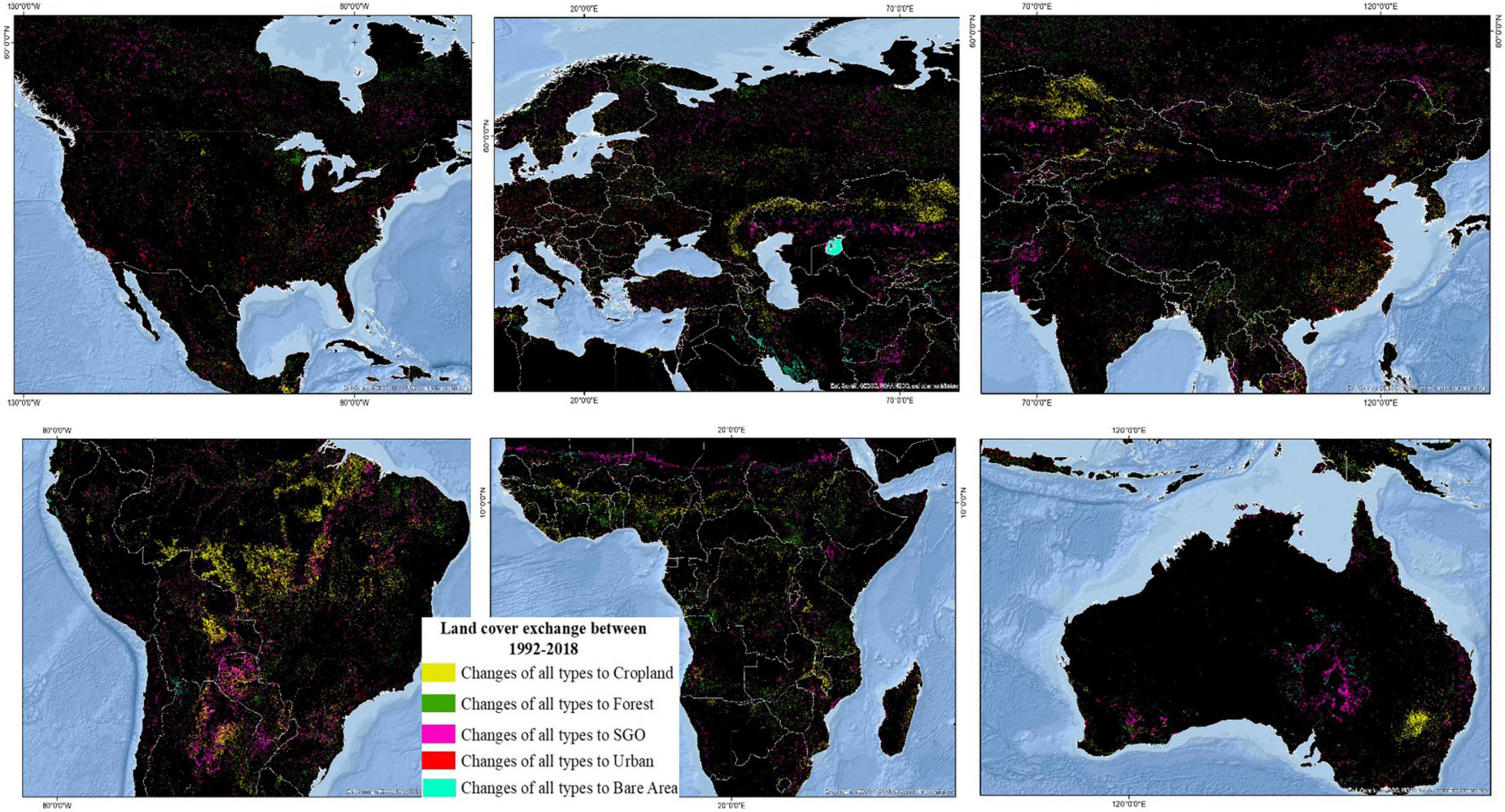
Figure 3. Maps of land-cover Exchanges (changes from the initial type to any other type) during the full period of 1992–2018.
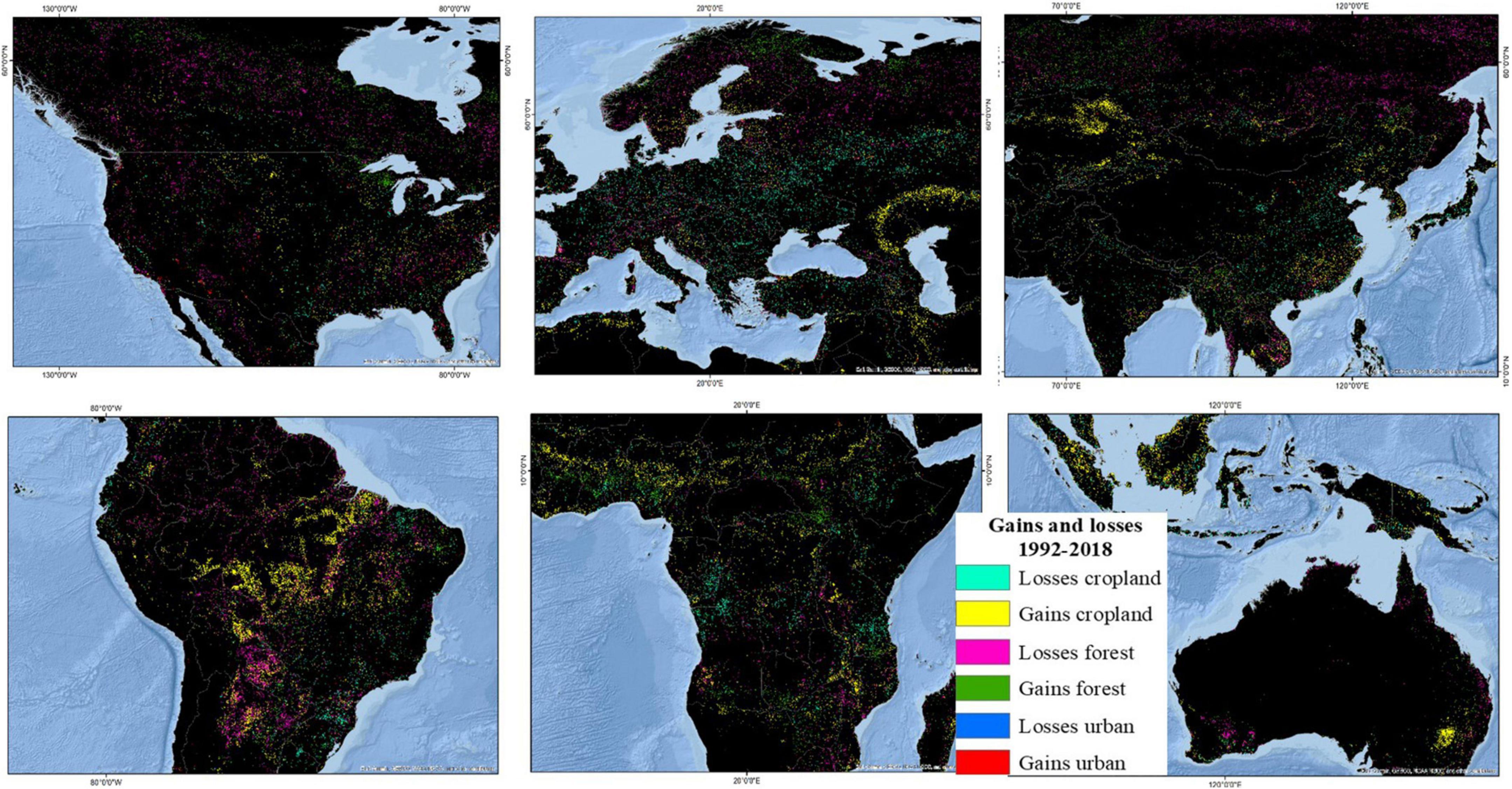
Figure 4. Maps of the main land-cover type gains and losses between 1992 and 2018.
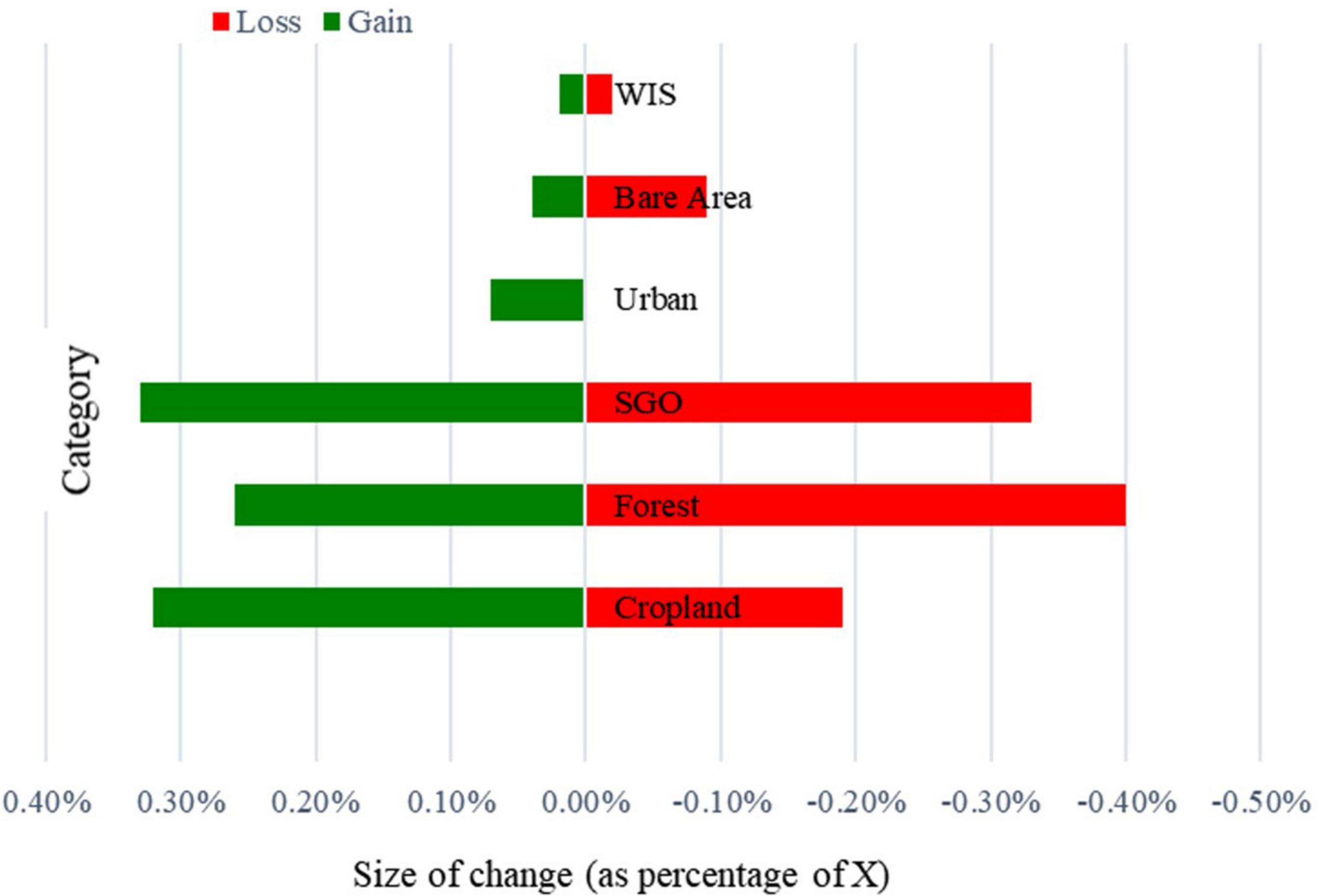
Figure 5. The losses and gains for each land-cover type during the entire study period.
The transitions that occurred between the six main land-cover types, where the diameters of the filled circles in Figure 1 represent the area of land that has undergone each transition, are expressed in square kilometers relative to the total area of land globally that changed land cover type over the study period. Globally, the largest transition is 1194912.4 km2 (17%) for the conversion of Forest cover to Cropland, followed by 651492.5 km2 (9.3%) for the conversion of Cropland to Forest cover, and 286650.4 km2 (4.1%) for the conversion of Cropland to Urban.
The estimated land-cover changes at the continental level during the individual time periods are expressed in Figure 6. Thus, summing the results for each land-type category in Asia over the entire time period of 1992–2018 indicates that Cropland and Urban expanded by 0.55% (243,704 km2) and 0.43% (191,776 km2), respectively, while Forest and Bare areas have declined by 0.68% (299,124 km2) and 0.36% (161,196 km2), respectively. Meanwhile, the continent of Africa experienced decreases of 0.31% (115,844 km2) in Bare area, and increases of 0.68% (205,576 km2) and 0.21% (65,348 km2) in Cropland and Forest, respectively. In Europe Urban has increased by 0.42% (97,704 km2), while Forest and Cropland have decreased by 0.77% (176,528 km2) and 0.32% (74,756 km2), respectively. In North America, Forest decreased by 0.30% (72,460 km2) while Urban and Cropland increased by 0.33% (79,952 km2) and 0.11% (27,968 km2), respectively. In South America, Cropland and Urban increased by 2.07% (368,384 km2) and 0.27% (23,280 km2), respectively, while Forest decreased by 3.2% (579,108 km2). Also, in Australia and Oceania, Cropland increased by 0.40% (34,120 km2), while Bare Area and Forest declined by 0.42% (34,780 km2) and 0.24% (20,484 km2), respectively.
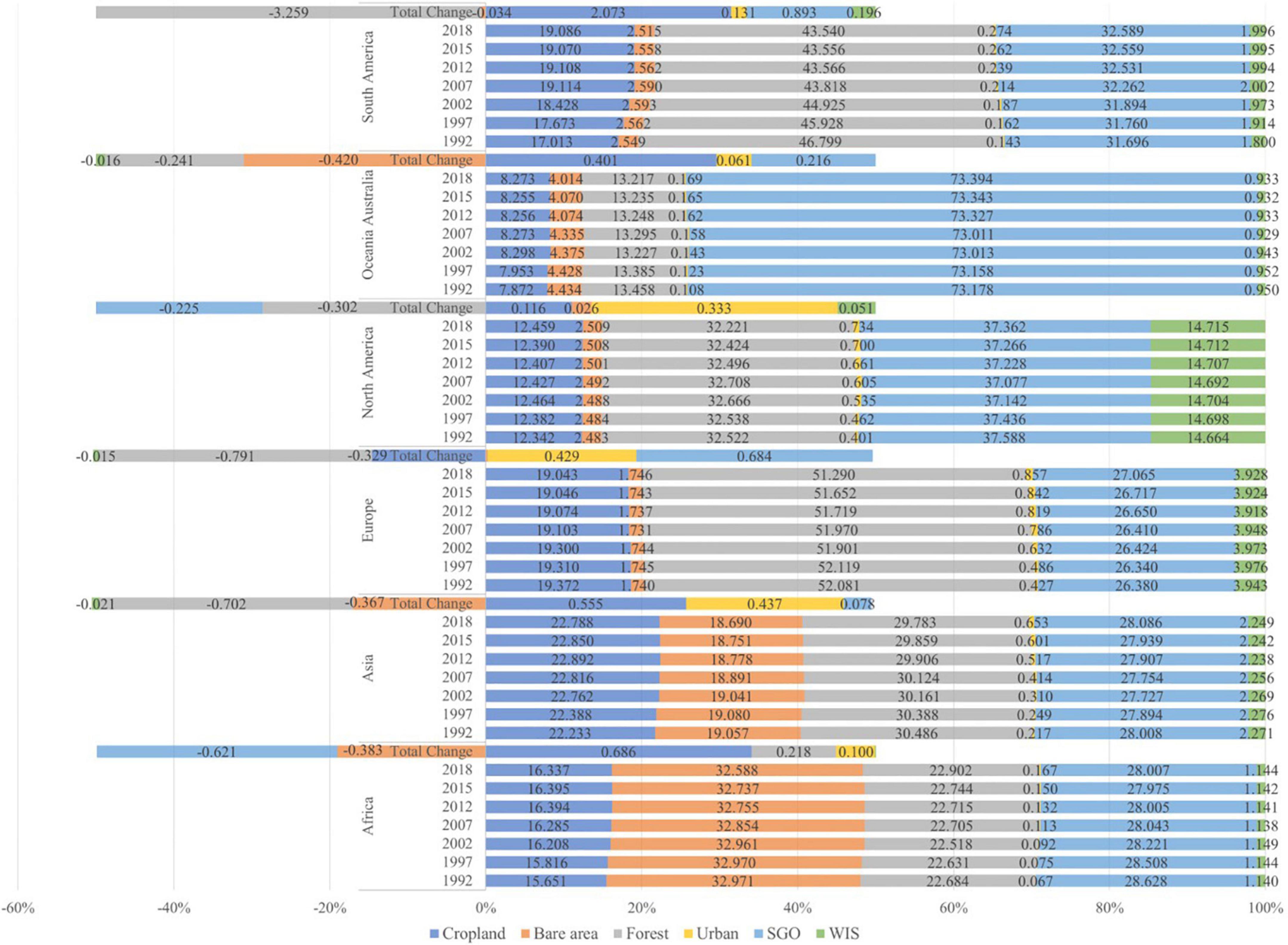
Figure 6. The percentage land-cover changes for each year by continent.
As global warming caused by human activity has led to changes in the distribution of climatic zones (especially an expansion of arid climates and a contraction of polar climates), the primary objective of this section is to examine how the various land cover types have changed in each climatic zone. It is anticipated that ongoing global warming will lead to the development of new, hot climates in tropical regions, along with a poleward movement of the climatic zones from middle to high latitudes, and increase in altitude for climatic zones at higher elevations. It is possible for ecosystems in these regions to undergo structural, compositional, and functional changes as a result of increased exposure to temperature and rainfall extremes that go beyond their accustomed climatic regimes. In addition, it is anticipated that warming at high latitudes may hasten the process of permafrost thawing, and raise the level of disturbance in boreal forests caused by both abiotic (such as drought and fire) and biotic (such as pests and disease) agents (Jia et al., 2019). Although Wang et al. (2019) have studied the land surface temperature throughout the period of increase, the spatial distribution of this increase has been influenced by the transformation in land cover, and needs to be considered. Hence, the present study compares the results from image classifications to estimate the changes that have occurred in the arid, cold, polar, and temperate tropical climate zones. In addition, a sixth category termed WIS is analyzed at the climatic level because this category includes water and snow, which are greatly affected by weather or climatic conditions. As shown in Figure 7, the tropical zones have experienced unprecedented rates of disturbance and conversion throughout their range. Between 1992 and 2018, tropical zones witnessed a 1.87% increase in Cropland and a 0.18% increase in Urban, while Forest decreased by 1.91%. Meanwhile, arid zones experienced increases of 0.38%, and 0.15% in Cropland and Urban, respectively, along with a 0.64% decrease in Bare area and a 0.02% decrease in Forest. In the temperate zones, Forest has declined by 0.99%, while Urban and Cropland increased by 0.85 and 0.08%, respectively. The cold regions experienced an increase of 0.35% in Urban cover, and an increase of 0.21% in Cropland, whereas Forest decreased by 0.52%. In the polar regions, Forest decreased by 0.01%.
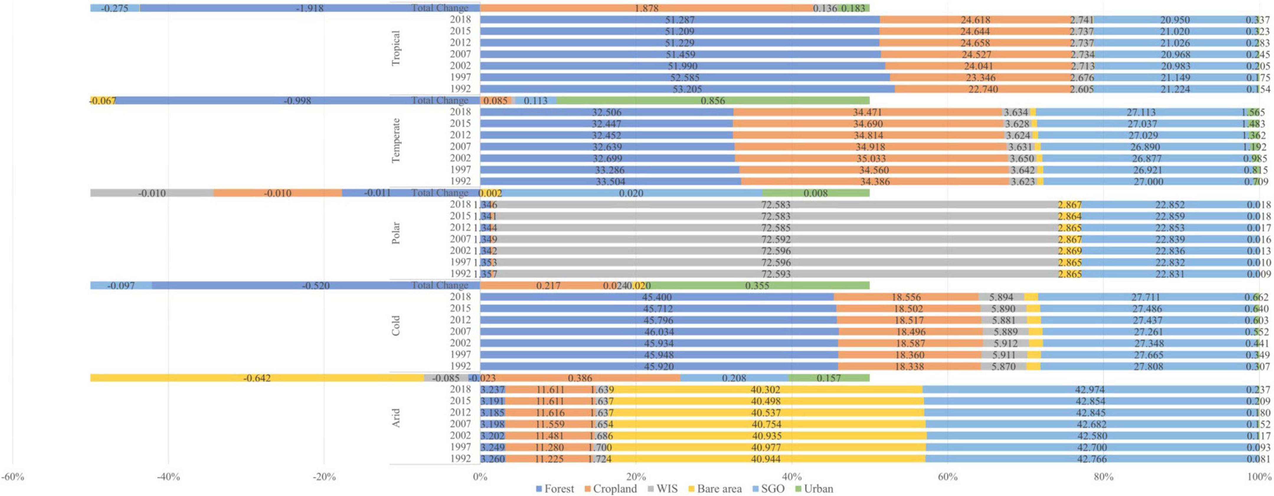
Figure 7. The percentage land-cover changes for each year by climatic zone.
Categorical level intensity provides information concerning the magnitudes of a category’s gross gains and losses, which is critical for explaining how a category’s change compares to its size at the beginning of a time interval. The present study shows that Cropland was an active gainer during the third, fourth, and fifth study time intervals, which is consistent with the findings of Cao et al. (2019), Liu et al. (2021), and Potapov et al. (2022). Meanwhile, Forest has been an active loser during all time intervals, which is consistent with the results of d’Annunzio et al. (2015), and can be ascribed to the logging of trees and clearing of forest areas in regions such as South America (Bilintoh, 2022). The Forest and SGO categories experienced both active gains and losses during various time intervals within the study period, with the positive changes resulting from ongoing projects aimed at restoring damaged forests in previously cleared areas across the globe. Urban was an active gainer during all the time intervals, we hypothesize that this mainly due to increased land requirements for infrastructural development in response to an increase in population growth rates. Expanded urban land use is needed in order to meet the basic living requirements of residents, including education and infrastructure. Hence, the United Nations has proposed sustainable development goals that include education, infrastructure, health, climate, and food security (United Nations, 2015).
As indicated by the pie charts in Figure 1, the net losses and gains in Bare area was dormant during all time intervals, even though changes may be expected to arise due to the various natural or artificial processes. For instance, change in sea levels may cause a cyclic pattern of gains and losses in sand and rock, which often characterize the landscapes around water bodies. Furthermore, natural disasters such as fire outbreaks in vegetated areas followed by regrowth of vegetation can contribute to loss and gains of Bare areas. The observed dormancy during all time intervals suggests that the various processes have an overall balancing influence.
According to previous studies, the LCC indicates a decrease in the mean and extreme global precipitation, particularly above regions of intense deforestation (Sy and Quesada, 2020; Hoang and Kanemoto, 2021). In addition, researchers have observed the more formal response of extreme weather conditions to the LCC (Findell et al., 2017; Lejeune et al., 2018). In those studies, the area of Cropland exhibited an increase between 1992 and 2012, but decreased between 2012 and 2018 (FAO, 2016). Similar observations have been made by Folberth et al. (2020). Some researchers have suggested that Cropland expansion must stop (e.g., Cunningham et al., 2013), but this would negatively affect the ability to secure nutritious food for people in the poorest parts of the globe McGuire (2015). Additionally, researchers have found that the global Cropland area increased by 110% between 1850 and 2015, while the area of the world’s forests decreased by 17% (Houghton and Nassikas, 2017). Similarly, the present study has revealed a continuous increase in the Urban area over the entire study time interval, which is in agreement with previous findings (Pesaresi et al., 2015; Liu et al., 2018, 2020; Gao and O’Neill, 2020; Lim et al., 2020). Moreover, these findings have been echoed more recently by van Vliet (2019), who found that 38.0 Mha of new cities were created between 1992 and 2015 worldwide, which represents an 115% increase during the last 23 years.
On a continental scale, the smallest decrease in Forest (0.77%) occurred in Europe majority of Russia, while South America experienced the largest decrease (3.2%) in Forest. Indeed, Africa was the only continent to have experienced an increase in Forest (0.21%). Similar results have been reported by Fearnside (2005), Nepstad et al. (2014), and Qin et al. (2019) as the rate of land-use change, anthropogenic activities, and climatic change in the Amazon have led to significant deforestation in the region over the years. As the biggest tropical forest worldwide, and the most complex terrestrial ecosystem, the Amazon is an important land for world conservation, and, as a result, should be closely monitored for anthropogenic impacts (Jenkins et al., 2013; Cavalcante et al., 2022). Meanwhile, Urban areas increased in all continents during 1992–2018, which is attributable to the impact of global urbanization. This has been especially prominent in Asia, Africa, and Europe.
In terms of climatic zones, the present study has revealed a substantial increase in Cropland within the tropical zone relative to the other zones during 1992–2018. This trend is related to the favorable conditions for farming, and the decrease in forests. Researchers have identified tropical deforestation as an increasingly common anthropogenic greenhouse gas source (van der Werf et al., 2009; Smith et al., 2014; Page et al., 2022), and other researchers have identified international trade as the most important driver of carbon emissions from tropical deforestation, over and above that caused by fossil fuels (Pendrill et al., 2019). In the present study, the temperate zone exhibited the most growth in Urban area and the greatest decrease in Forest between 1992 and 2018. This is an interesting finding, and it can be hypothesized that the decreased Forest resulted in increased Urban and Cropland during 2012–2018. Meanwhile, the arid zone experienced a major decrease in Bare areas, but the largest increase in Cropland. Our results also confirm other studies that suggested that Bare area decreased by 0.06% overall globally, but decreased differently between continents. Similar observations were previously reported by Song et al. (2018), who found that Bare area was reduced by 1.16 million km2 (3.1%) worldwide, but most significantly in the agrarian regions of Asia. Meanwhile, Forest cover in Asia has continuously decreased, while Urban cover has increased, during the last 26 years.
The present investigation was performed without any major problems; nevertheless, there were some restrictions. The technical significance of the research design and the methods of data analysis were discussed, and recommendations were made for future research at the global scale, particularly big data. For a global intensity and net change analysis, high-quality data should be selected, divided into sections, and then combined. When calculating the intensity and net change for global analysis, it is important to proceed very carefully, as errors can be introduced at each step, and accumulate.
This paper aimed to monitor land cover change on a global scale, by making use of the unique data on global land cover change. We first reclassified data globally, then evaluated their intensity analysis categorical level for six time intervals 1992–1997, 1997–2002, 2002–2007, 2007–2012, and 2012–2018. Afterward, we assessed changes in land use in 1992, 1997, 2002, 2007, 2012, 2015, and 2018 by continent and climate zone. Additionally, the global land-cover changes in the six land cover type were analyzed according to specific continental and climatic zones. Instead of focusing only on one specific land cover transition or specific regions, as was the case in most previous studies, our research involved all possible transitions at a global scale. Also, this is the first time change intensity analysis was conducted globally.
A thorough spatio-temporal approach was developed for analyzing and acquiring an improved understanding of the global land-cover change in terms of the intensities of three components (Quantity, Exchange, and Shift) for six different land-cover categories between 1992 and 2018. The results revealed that the Exchange component accounted for most of the change in all categories except for Urban, which experienced predominantly Quantity change. Notably, Bare area experienced a gross loss after the first time interval (1992–1997), while Cropland experienced gross gains during all time intervals except for 2012–2018. Urban areas experienced gross gains during every time interval, and this is directly associated with continuous gross losses in Forest and Bare area. Furthermore, the intensity of Urban change was active during all the time intervals, which can be attributed to an increase in the human population and, hence, the need for expansion in infrastructural developments such as housing. The intensity analysis assessed the processes of land-use change by defining the concept of stability. Although the creation of stable land use might not automatically lead to sustainable development, it can provide a strong basis for the development of sustainability.
Cropland increased in Asia, Africa, and Europe during the period 1992–2012, and then decreased from 2012 to 2018, while Shrubland decreased during 1992–2012, but increased during 2012–2018. Another positive finding from this study is that North America and Europe have experienced decreases in the area of Bare land since 2000, while hotspots of Bare area continuously increased throughout the study period in other regions.
Over the past 3 years, the total area of Forest has increased in tropical, temperate, and arid climatic zones, but decreased in the cold climatic zone. Concurrently, the tropical and temperate climatic zones each exhibited a lower decrease in Cropland, while the arid and cold zones experienced increases in Cropland.
The results presented provide critical supporting information on the active change that is needed for climate change adaptation. Moreover, the findings can provide critical information for promoting progress toward the UN’s Sustainable Development Goals (SDGs), and can assist policymakers in regulating future land use change in a sustainable manner.
The original contributions presented in this study are included in the article/supplementary material, further inquiries can be directed to the corresponding author.
ML and TB: plan methodology and evaluate results, writing, and review. ML: writing original draft preparation. ML and C-HL: editing. All authors have read and agreed to the published version of the manuscript.
This research was funded by the National Research Foundation of Korea (NRF) grant provided by the Ministry of Education (No. 2021R1I1A1A01060652), the Ministry of Science and ICT (No. 2022R1C1C1008489), and Kookmin University grant.
The authors declare that the research was conducted in the absence of any commercial or financial relationships that could be construed as a potential conflict of interest.
All claims expressed in this article are solely those of the authors and do not necessarily represent those of their affiliated organizations, or those of the publisher, the editors and the reviewers. Any product that may be evaluated in this article, or claim that may be made by its manufacturer, is not guaranteed or endorsed by the publisher.
Aldwaik, S. Z., and Pontius, R. G. Jr. (2012). Intensity analysis to unify measurements of size and stationarity of land changes by interval, category, and transition. Landscape Urban Plan. 106, 103–114. doi: 10.1016/j.landurbplan.2012.02.010
Alkama, R., and Cescatti, A. (2016). Biophysical climate impacts of recent changes in global forest cover. Science 351, 600–604. doi: 10.1126/science.aac8083
Amin, A., and Fazal, S. (2012). Land transformation analysis using remote sensing and GIS techniques (a case study). J. Geogr. Inf. Syst. 4, 229–236. doi: 10.4236/jgis.2012.43027
Bilintoh, T. M. (2022). Intensity Analysis to Analyze the Dynamics of Reforestation in the Rio Deco Water Basin. Front. Remote Senses. 3:873341. doi: 10.3389/frsen.2022.873341
Bonan, G. B. (2008). Forests and climate change: Forcings, feedbacks, and the climate benefits of forests. Science 320, 1444–1449. doi: 10.1126/science.1155121
Brovkin, V., Boysen, L., Arora, V. K., Boisier, J. P., Cadule, P., Chini, L., et al. (2013). Effect of anthropogenic land-use and land-cover changes on climate and land carbon storage in CMIP5 projections for the twenty-first century. J. Clim. 26, 6859–6881. doi: 10.1175/JCLI-D-12-00623.1
Cao, M., Zhu, Y., Quan, J., Zhou, S., Lü, G., Chen, M., et al. (2019). Spatial sequential modeling and predication of global land use and land cover changes by integrating a global change assessment model and cellular automata. Earth’s Future 7, 1102–1116. doi: 10.1029/2019EF001228
Cavalcante, R. B. L., Nunes, S., Viademonte, S., Rodrigues, C. M. F., Gomes, W. C., and da Silva Ferreira Jr., et al. (2022). Multicriteria approach to prioritize forest restoration areas for biodiversity conservation in the eastern Amazon. J. Environ. Manage. 318:115590. doi: 10.1016/j.jenvman.2022.115590
Chen, H., and Gilmore Pontius, R. (2011). Sensitivity of a land change model to pixel resolution and precision of the independent variable. Environ. Modeling Assess. 16, 37–52.
Cloern, J. E., Abreu, P. C., Carstensen, J., Chauvaud, L., Elmgren, R., Grall, J., et al. (2016). Human activities and climate variability drive fast-paced change across the world’s estuarine–coastal ecosystems. Global Change Biol. 22, 513–529. doi: 10.1111/gcb.13059
Cunningham, S. A., Attwood, S. J., Bawa, K. S., Benton, T. G., Broadhurst, L. M., Didham, R. K., et al. (2013). To close the yield-gap while saving biodiversity will require multiple locally relevant strategies. Agr. Ecosyst. Environ. 173, 20–27. doi: 10.1016/j.agee.2013.04.007
d’Annunzio, R., Sandker, M., Finegold, Y., and Min, Z. (2015). Projecting global forest area towards 2030. For. Ecol. Manag. 352, 124–133. doi: 10.1016/j.foreco.2015.03.014
Di Gregorio, A. (2005). Land Cover Classification System: Classification Concepts and User Manual: LCCS. Rome: Food and Agriculture Org.
ESA (2017). Land cover, CCI. Product user Guide Version 2.0. Available online at: http://maps.elie.ucl.ac.be/CCI/viewer/download/ESACCI-LC-Ph2-PUGv2_2.0.pdf, last access: 10 November. (2017).
ESA (2020). Climate change initiative extension (CCI+) phase 1 new essential climate variables (NEW ECVS) high resolution land cover ECV (HR_LandCover_cci). Available online at: https://climate.esa.int/media/documents/CCI_HRLC_Ph1-D2.2_ATBD_v2.0.pdf
Fang, J., Yu, G., Liu, L., Hu, S., and Chapin, F. S. III. (2018). Climate change, human impacts, and carbon sequestration in China. Proc. Natl. Acad. Sci. 115, 4015–4020. doi: 10.1073/pnas.1700304115
FAO (2016). Food and Agriculture Organization of the United Nations. Rome: Food Agriculture Organization.
Fearnside, P. M. (2005). Deforestation in Brazilian Amazonia: History, rates, and consequences. Conserv. Biol. 19, 680–688. doi: 10.1111/j.1523-1739.2005.00697.x
Feng, Y., Lei, Z., Tong, X., Gao, C., Chen, S., Wang, J., et al. (2020). Spatially-explicit modeling and intensity analysis of China’s land use change 2000–2050. J. Environ. Manage. 263:110407. doi: 10.1016/j.jenvman.2020.110407
Findell, K. L., Berg, A., Gentine, P., Krasting, J. P., Lintner, B. R., Malyshev, S., et al. (2017). The impact of anthropogenic land use and land cover change on regional climate extremes. Nat. Commun. 8:989. doi: 10.1038/s41467-017-01038-w
Folberth, C., Khabarov, N., Balkovič, J., Skalský, R., Visconti, P., Ciais, P., et al. (2020). The global cropland-sparing potential of high-yield farming. Nat. Sustain. 3, 281–289. doi: 10.1038/s41893-020-0505-x
Foley, J. A., DeFries, R., Asner, G. P., Barford, C., Bonan, G., Carpenter, S. R., et al. (2005). Global Consequences of Land Use. Science 309, 570–574. doi: 10.1126/science.1111772
Gao, J., and O’Neill, B. C. (2020). Mapping global urban land for the 21st century with data-driven simulations and Shared Socioeconomic Pathways. Nat. Commun. 11:2302. doi: 10.1038/s41467-020-15788-7
Gaspari, F. J., Delgado, M. I., and Denegri, G. A. (2009). Spatial, Temporal and Economic Estimation of Soil Loss from Surface Water Erosion. Terra Latinoamericana 27, 43–51.
Ghimire, B., Williams, C. A., Masek, J., Gao, F., Wang, Z., Schaaf, C., et al. (2014). Global albedo change and radiative cooling from anthropogenic land cover change, 1700 to 2005 based on MODIS, land use harmonization, radiative kernels, and reanalysis. Geophys. Res. Lett. 41, 9087–9096. doi: 10.1002/2014GL061671
Gontier, M., Mörtberg, U., and Balfors, B. (2010). Comparing GIS-based habitat models for applications in EIA and SEA. Environ. Impact Assess. Rev. 30, 8–18. doi: 10.1016/j.eiar.2009.05.003
Hoang, N. T., and Kanemoto, K. (2021). Mapping the deforestation footprint of nations reveals growing threat to tropical forests. Nat. Ecol. Evol. 5, 845–853. doi: 10.1038/s41559-021-01417-z
Houghton, R. A., and Nassikas, A. A. (2017). Global and regional fluxes of carbon from land use and land cover change 1850–2015. Global Biogeochem. 31, 456–472. doi: 10.1002/2016GB005546
Jenkins, C. N., Pimm, S. L., and Joppa, L. N. (2013). Global patterns of terrestrial vertebrate diversity and conservation. Proc. Natl. Acad. Sci. 110, E2602–E2610. doi: 10.1073/pnas.1302251110
Jepsen, M. R., Kuemmerle, T., Müller, D., Erb, K., Verburg, P. H., Haberl, H., et al. (2015). Transitions in European land-management regimes between 1800 and 2010. Land Use Policy 49, 53–64. doi: 10.1016/j.landusepol.2015.07.003
Jia, G., Shevliakova, E., Artaxo, P., De Noblet-Ducoudré, N., Houghton, R., House, J., et al. (2019). Land–Climate Interactions: Climate Change and Land An IPCC Special Report on Climate Change, Desertification, Land Degradation, Sustainable Land Management, Food Security, and Greenhouse Gas Fluxes in Terrestrial Ecosystems. Geneva: IPCC.
Khoi, D. D., and Murayama, Y. (2010). Forecasting areas vulnerable to forest conversion in the Tam Dao National Park Region Vietnam. Remote Sens. 2, 1249–1272. doi: 10.3390/rs2051249
Klein Goldewijk, K. (2016). A Historical Land Use Data Set for the Holocene; HYDE 3.2. Utrecht University: EGU General Assembly Conference Abstracts, ESC2016–ESC1574. doi: 10.5194/essd-9-927-2017
Klein Goldewijk, K., Beusen, A., Van Drecht, G., and De Vos, M. (2011). The HYDE 3.1 spatially explicit database of human-induced global land-use change over the past 12,000 years. Global Ecol. Biogeogr. 20, 73–86. doi: 10.1111/j.1466-8238.2010.00587.x
Lamchin, M., Wang, S. W., Lim, C. H., Ochir, A., Pavel, U., Gebru, B. M., et al. (2020). Understanding global spatio-temporal trends and the relationship between vegetation greenness and climate factors by land cover during 1982–2014. Glob. Ecol. Conserv. 24:e01299. doi: 10.1016/j.gecco.2020.e01299
Lejeune, Q., Davin, E. L., Gudmundsson, L., Winckler, J., and Seneviratne, S. I. (2018). Historical deforestation locally increased the intensity of hot days in northern mid-latitudes. Nat. Clim. Change 8, 386–390. doi: 10.1038/s41558-018-0131-z
Lim, C. H., Ryu, J., Choi, Y., Jeon, S. W., and Lee, W. K. (2020). Understanding global PM2. 5 concentrations and their drivers in recent decades (1998–2016). Environ. Int. 144:106011. doi: 10.1016/j.envint.2020.106011
Liu, M., and Tian, H. (2010). China’s land cover and land use change from 1700 to 2005: Estimations from high-resolution satellite data and historical archives. Global Biogeochem. 24:GB3003. doi: 10.1029/2009GB003687
Liu, X., Hu, G., Chen, Y., Li, X., Xu, X., Li, S., et al. (2018). High-resolution multi-temporal mapping of global urban land using Landsat images based on the Google Earth Engine Platform. Remote Sens. Environ. 209, 227–239. doi: 10.1016/j.rse.2018.02.055
Liu, X., Huang, Y., Xu, X., Li, X., Li, X., Ciais, P., et al. (2020). High-spatiotemporal-resolution mapping of global urban change from 1985 to 2015. Nat. Sustain. 3, 564–570. doi: 10.1038/s41893-020-0521-x
Liu, Z., Liu, Y., and Wang, J. (2021). A global analysis of agricultural productivity and water resource consumption changes over cropland expansion regions. Agric. Ecosyst. Environ. 321:107630. doi: 10.1016/j.agee.2021.107630
McGuire, S. (2015). FAO, IFAD, and WFP. The state of food insecurity in the world 2015: Meeting the 2015 international hunger targets: Taking stock of uneven progress. Rome: FAO, 2015. Adv. Nutr. 6, 623–624. doi: 10.3945/an.115.009936
Mendoza-Ponce, A., Corona-Nunez, R., Kraxner, F., Leduc, S., and Patrizio, P. (2018). Identifying effects of land use cover changes and climate change on terrestrial ecosystems and carbon stocks in Mexico. Glob. Environ. Change 53, 12–23. doi: 10.1016/j.gloenvcha.2018.08.004
Mishra, V. N., Rai, P. K., and Mohan, K. (2014). Prediction of land use changes based on land change modeler (LCM) using remote sensing: A case study of Muzaffarpur (Bihar), India. J. Geogr. Inst. Jovan Cvijic SASA 60, 111–127. doi: 10.2298/IJGI1401111M
Nepstad, D., McGrath, D., Stickler, C., Alencar, A., Azevedo, A., Swette, B., et al. (2014). Slowing Amazon deforestation through public policy and interventions in beef and soy supply chains. Science 344, 1118–1123. doi: 10.1126/science.1248525
Olmedo, M. T. C., Pontius, R. G. Jr., Paegelow, M., and Mas, J. F. (2015). Comparison of simulation models in terms of quantity and allocation of land change. Environ. Modell. Softw. 69, 214–221. doi: 10.1016/j.envsoft.2015.03.003
Olivier, A., Jose Ramos, P., Vasileios, K., Pierre, D., and Frederic, A. (2010). “GlobCover 2009,” in Proceedings of ESA living planet symposium, held on 28 June - 2 July 2010, Bergen.
Page, S., Mishra, S., Agus, F., Anshari, G., Dargie, G., Evers, S., et al. (2022). Anthropogenic impacts on lowland tropical peatland biogeochemistry. Nat. Rev. Earth Environ. 3, 426–443. doi: 10.1038/s43017-022-00289-6
Pandolfi, G. S. (2016). Effects of Climate, Land Use and in-Stream Habitat on Appalachian Elktoe (Alasmidonta Raveneliana) in the Nolichucky River Drainage, Ph.D thesis, North Carolina: Appalachian State University
Patel, N., and Kaushal, B. K. (2010). Improvement of user’s accuracy through classification of principal component images and stacked temporal images. Geo Spat. Inf. Sci. 13, 243–248. doi: 10.1007/s11806-010-0380-0
Pendrill, F., Persson, U. M., Godar, J., Kastner, T., Moran, D., Schmidt, S., et al. (2019). Agricultural and forestry trade drives large share of tropical deforestation emissions. Global Environ. Change 56, 1–10. doi: 10.1016/j.gloenvcha.2019.03.002
Pesaresi, M., Ehrilch, D., Florczyk, A. J., Freire, S., Julea, A., Kemper, T., et al. (2015). GHS Built-Up Grid, Derived from Landsat, Multitemporal (1975, 1990, 2000, 2014). Belgium: European Commission.
Pickard, B., Gray, J., and Meentemeyer, R. (2017). Comparing quantity, allocation and configuration accuracy of multiple land change models. Land 6:52. doi: 10.3390/land6030052
Pontius, R. G. Jr., Gao, Y., Giner, N. M., Kohyama, T., Osaki, M., and Hirose, K. (2013). Design and interpretation of intensity analysis illustrated by land change in Central Kalimantan Indonesia. Land 2, 351–369. doi: 10.3390/land2030351
Potapov, P., Turubanova, S., Hansen, M. C., Tyukavina, A., Zalles, V., Khan, A., et al. (2022). Global maps of cropland extent and change show accelerated cropland expansion in the twenty-first century. Nat. Food 3, 19–28. doi: 10.1038/s43016-021-00429-z
Qin, Y., Xiao, X., Dong, J., Zhang, Y., Wu, X., Shimabukuro, Y., et al. (2019). Improved estimates of forest cover and loss in the Brazilian Amazon in 2000–2017. Nat. Sustain. 2, 764–772. doi: 10.1038/s41893-019-0336-9
Quan, B., Pontius, R. G. Jr., and Song, H. (2019). Intensity Analysis to communicate land change during three time intervals in two regions of Quanzhou City, China. GIsci. Remote Sens. 57, 21–36. doi: 10.1080/15481603.2019.1658420
Sang, X., Guo, Q., Wu, X., Fu, Y., Xie, T., He, C., et al. (2019). Intensity and stationarity analysis of land use change based on CART algorithm. Sci. Rep. 9:12279. doi: 10.1038/s41598-019-48586-3
Shafizadeh-Moghadam, H., Minaei, M., Feng, Y., and Pontius, R. G. Jr. (2019). GlobeLand30 maps show four times larger gross than net land change from 2000 to 2010 in Asia. Int. J. Appl. Earth Obs. 78, 240–248. doi: 10.1016/j.jag.2019.01.003
Shrestha, S., Bhatta, B., Shrestha, M., and Shrestha, P. K. (2018). Integrated assessment of the climate and landuse change impact on hydrology and water quality in the Songkhram River Basin Thailand. Sci. Total Environ. 643, 1610–1622. doi: 10.1016/j.scitotenv.2018.06.306
Smith, P., Clark, H., Dong, H., Elsiddig, E. A., Haberl, H., Harper, R., et al. (2014). “Agriculture, forestry and other land use (AFOLU),” in Climate Change 2014: Mitigation of Climate Change Contribution of Working Group III to the Fifth Assessment Report of the Intergovernmental Panel on Climate Change, eds O. Edenhofe, R. Pichs-Madruga, Y. Sokona, E. Farahani, S. Kadner, and K. Seyboth (Cambridge, UK: Cambridge University Press), 811–922. doi: 10.1017/CBO9781107415416.017
Song, X. P., Hansen, M. C., Stehman, S. V., Potapov, P. V., Tyukavina, A., Vermote, E. F., et al. (2018). Global land change from 1982 to 2016. Nature 560, 639–643. doi: 10.1038/s41586-018-0411-9
Sy, S., and Quesada, B. (2020). Anthropogenic land cover change impact on climate extremes during the 21st century. Environ. Res. Lett. 15:034002. doi: 10.1088/1748-9326/ab702c
Teixeira, Z., Marques, J. C., and Pontius, R. G. Jr. (2016). Evidence for deviations from uniform changes in a Portuguese watershed illustrated by CORINE maps: An intensity analysis approach. Ecol. Indic. 66, 382–390. doi: 10.1016/j.ecolind.2016.01.018
Tsai, Y., Zia, A., Koliba, C., Guilbert, J., Bucini, G., and Beckage, B. (2013). “Impacts of land managers’ decisions on landuse transition within Missisquoi Watershed Vermont: An application of agent-based modeling system,” in 2013 IEEE International Systems Conference (SysCon), (New York, NY: IEEE), 824–829. doi: 10.1109/SysCon.2013.6549979
United Nations, (2015). Sustainable Development Goals. Available online at: https://sustainabledevelopment.un.org/sdgs. United Nations (UN). (accessed August 22, 2022).
Václavík, T., and Rogan, J. (2009). Identifying trends in land use/land cover changes in the context of post-socialist transformation in central Europe: A case study of the greater Olomouc region Czech Republic. GISci. Remote Sens. 46, 54–76. doi: 10.2747/1548-1603.46.1.54
van der Werf, G. R., Morton, D. C., DeFries, R. S., Oliver, J. G. J., Kasibhatla, P., Jackson, R. B., et al. (2009). C02 emissions from deforestation. Nat. Geosci. 2, 737–738. doi: 10.1038/ngeo671
van Vliet, J. (2019). Direct and indirect loss of natural area from urban expansion. Nat. Sustain. 2, 755–763. doi: 10.1038/s41893-019-0340-0
Veldkamp, A., and Verburg, P. H. (2004). Modelling land use change and environmental impact. J. Environ. Manage. 72, 1–3. doi: 10.1016/j.jenvman.2004.04.004
Wang, J., Chen, Y., Shao, X., Zhang, Y., and Cao, Y. (2012). Land-use changes and policy dimension driving forces in China: Present, trend and future. Land Use Policy 29, 737–749. doi: 10.1016/j.landusepol.2011.11.010
Keywords: global land cover, intensity analysis, land cover change, loss and gain, categorical analysis
Citation: Lamchin M, Bilintoh TM, Lee W-K, Ochir A and Lim C-H (2022) Exploring spatio-temporal change in global land cover using categorical intensity analysis. Front. For. Glob. Change 5:994713. doi: 10.3389/ffgc.2022.994713
Received: 15 July 2022; Accepted: 26 September 2022;
Published: 11 October 2022.
Edited by:
Barry Alan Gardiner, Institut Européen De La Forêt Cultivée (IEFC), FranceReviewed by:
Gopal Shukla, Uttar Banga Krishi Viswavidyalaya, IndiaCopyright © 2022 Lamchin, Bilintoh, Lee, Ochir and Lim. This is an open-access article distributed under the terms of the Creative Commons Attribution License (CC BY). The use, distribution or reproduction in other forums is permitted, provided the original author(s) and the copyright owner(s) are credited and that the original publication in this journal is cited, in accordance with accepted academic practice. No use, distribution or reproduction is permitted which does not comply with these terms.
*Correspondence: Chul-Hee Lim, Y2xpbUBrb29rbWluLmFjLmty
Disclaimer: All claims expressed in this article are solely those of the authors and do not necessarily represent those of their affiliated organizations, or those of the publisher, the editors and the reviewers. Any product that may be evaluated in this article or claim that may be made by its manufacturer is not guaranteed or endorsed by the publisher.
Research integrity at Frontiers
Learn more about the work of our research integrity team to safeguard the quality of each article we publish.