Understanding the states and dynamics of mangrove forests in land cover transitions of The Gambia using a Fourier transformation of Landsat and MODIS time series in Google Earth Engine

Introduction: Mangroves are resilient forests of transitional zones between land, ocean and freshwater for they are tolerant to salinity. In The Gambia, mangrove forests are found along the coast of Atlantic Ocean and River Gambia where they support the livelihoods of millions through multiple ecosystems services. Despite their importance in The Gambia, consistent country-wide information on their coverage, dynamics and change hotspots are lacking. Thus far, it remains unclear whether the coverage of mangroves has decreased or increased over the last few decades. Often, the existing estimates vary strongly across sources and the methodologies in the available literature are not always reproducible. This study attempts to fill these gaps by providing up-to-date spatial information on mangrove forests in The Gambia.

Methods: To provide a reproducible workflow and a comprehensive assessment, we used continuous time series of freely available data to study the extent and dynamics of mangrove forests in The Gambia. To construct gap-free image time series, we used statistical models to describe land surface phenology based on monthly composites derived from Landsat and MODIS land surface reflectance acquired between 2000 and 2020. We used 1212 Landsat and 407 MODIS tiles spread across multiple spectral indices along with a calibrated set of training and validation data to train and validate a random forest classifier for accurate land cover classifications.

Results and discussion: The overall accuracy and Kappa statistics of the classifications range between 0.96 and 0.98. Our findings suggest a net increase of 4,000 ha in mangrove forests over the last 2 decades, corresponding to an annual rate of 200 ha. The net increase is largely due to strong policy making which results in participative forest resource management through the national forest action plan. The net increase in mangrove forests should not mask the substantial degradation in some places across the country. We estimated a total loss of nearly 5,670 ha, most of which appears to have taken place during the last decade in favor of wetlands. The Gambian mangroves are amongst the most promising green business in Gulf of Guinea, deserving an integrated governance - policy framework that address the key requirements for ecological sustainability.

Introduction

The Gambia has a sizeable area of mangroves that substantially contribute to rural livelihoods. These mangroves, estimated to extend up to 160 km from the coast along the River Gambia and covering an estimated area ranging between 497 and 747 km², are among the most developed mangroves of West Africa (Spalding et al., 1997; Feka and Ajonina, 2011; Ajonina et al., 2013). Among other functions, these mangroves provide food such as fish, oysters, and shrimps and also domestic products such as wood fuel and timber for construction and perform various regulatory functions such as coastal protection and carbon sink (UNEP, 2007b; Satyanarayana et al., 2012; Ceesay et al., 2017). There is a need to manage and monitor these mangroves for sustaining the valuable ecosystem goods and services they provide to the Gambians (Satyanarayana et al., 2012).

Despite the importance of these mangroves, the trend of mangrove vegetation in The Gambia for the past two decades remains unclear. The discrepancy among the available mangrove estimates in The Gambia implies potential problems in the remote sensing approaches that produce these estimates. An approach that addresses these problems would help to reduce these discrepancies and improve the accuracy of mangrove coverage and dynamics in The Gambia. We identified the major uncertainty factors that may have caused the discrepancies. Broadly, these include problems related to data sanity checks, variations in the scale of analysis, the use of non-standard classification systems, and differences in the classification algorithms.

The lack of continuous clear observations due to various remote sensing artifacts (e.g., clouds and cloud shadows) limits remote sensing applications to a few images with the best available number of clear pixels (Zhu and Woodcock, 2014; Zhu et al., 2015). Typically, the landscape, which presents strong intra-annual and inter-annual variabilities, is described using a single image at a given point in time. For analysis spanning more than a tile, it is often difficult to find a pair of clear tiles that are close in time. Such data specifications may not reasonably capture the true surface state variability since tropical LULC can present significant variability between years and between the times of the year. In using a single image approach, different studies may subjectively select different input images. Such a selective image specification will likely lead to different results, exacerbating the range of discrepancies between studies. Similarly, reference data (e.g., training data for image classification) for machine learning models can be easily flawed in the sense that fewer LULC than what is present on the ground is likely to result in an inaccurate classification that does not necessarily reflect the real ground conditions. In addition, the use of non-standard classification systems leads to arbitrary class labels making cross-study comparisons difficult. LULC classification system should be sufficiently detailed to detect the changes between mangroves and other forested covers. Studies aiming to provide accurate change estimates should consider all major LULCs while keeping the reference data consistent with the temporal change in these LULCs. Unless data are normalized to a comparable scale, reference data should be collected over the areas of persistent LULC.

While the spatial resolution seems to have minor importance in explaining the discrepancies in mangrove estimates in The Gambia, the difference in the spatial scale can be concerning when the base data do not sufficiently describe the temporal variability of the area of interest. The interpretations of mangrove dynamics in the region diverge because the scale of many remote sensing analyses does not always capture local accounts of mangrove cover gains and losses (Fent et al., 2019). Spalding et al. (1997) reported a decrease from 600 to < 500 km² between 1982 and 1995. UNEP (2007b) reported a slight decrease (from 747 in 1997 to 580 km² in 2005) in mangrove vegetation and attributed it to drought, increase in soil salinity, illegal exploitation, and land use conversion. Ceesay et al. (2017) estimated this decline in Tanbi Wetlands National Park of The Gambia at 6% between 1973 and 2012 and attributed it to increase salinity which negatively affects mangrove regrowth and rejuvenation. In the Central River Region of The Gambia, Ali Bah (2019) estimated this decline at 5.54% between 1984 and 1994, 7.18% between 1994 and 2007, and 22.02% between 2007 and 2017 and attributed it to an increase in temperature and a decrease in rainfall coupled with increased settlement and grazing land. In contrast, Fent et al. (2019) found an overall increase in mangrove forest areas of 51.21% between 1988 and 2018 across The Gambia and in the Sine Saloum and lower Casamance estuaries in Senegal. In these areas, mangroves have seen a significant recovery between 1988 and 1999 following the increased precipitation and tree species regrowth that experiences diebacks due to salinization caused by drought (Fent et al., 2019). While Sine Saloum experienced a lower precipitation increase between 1988 and 1999 compared to Low Casamance, the former has seen an important increase and the latter a slight decline in mangrove forests (Fent et al., 2019). It is clear from the studies that mangrove dynamics is a complex topic that requires multi-disciplinary approaches where various scale-dependent factors are required. Evidence from recent studies (Fent et al., 2019) has shown that neither climatic, political, and nor anthropogenic factors alone can explain the dynamic of mangrove vegetation near The Gambia and arguably elsewhere.

Besides the issues related to data sanity checks, classification systems, and classification algorithms, the reasons for these discrepancies in estimates can also be explained by the sporadic nature of the available studies which targeted different periods and scales of analysis. To the best of our knowledge, none of these studies succeeded in reconstructing the time series of satellite images due to various remote sensing artifacts in the region and limitations in computing resources for handling big data. With few exceptions (Fent et al., 2019), studies aiming at The Gambian mangroves have not been sufficiently holistic in the sense of explaining the dynamics of the biophysical settings in their specific context. While many studies (Jakubauskas and Legates, 2000; Zhu and Woodcock, 2014; Zhu et al., 2015) have successfully applied harmonic modeling (also known as Fourier analysis) against remote sensing artifacts, to remove noise or to achieve outstanding classification results elsewhere, most of the available estimates of mangrove areas and trends in The Gambia proceed via the comparisons of image classifications derived from single-point images. Many problems can arise. Because mangroves can be easily confused with other ecological systems (e.g., closed forests and riparian vegetation), studies aiming to provide realistic estimates of mangrove dynamics should accurately account for spatial and temporal variabilities of coastal ecosystems (Fent et al., 2019).

The objective of this study was to assess mangrove dynamics in The Gambia. We used a locally continuous time series of remotely sensed images to map all major land use and land covers (LULCs) while putting emphasis on mangrove forest dynamics in The Gambia.

Materials and methods

Study area

The Gambia (Figure 1) is located on the Gulf of Guinea, bordered by the Atlantic Ocean to the west while forming an enclave within Senegal. The country has an area of around 10,689 km² (11,300 km² River Gambia included) extending 320 km along the Gambia River. The country is subdivided into 5 administrative units including the Western Region, North Bank Region, Lower River Region, Central River Region, and the Upper River Region.

FIGURE 1

Figure 1. Overview of The Gambia. The red box indicates the bounding box of the country used as a reference for data collection in a spatial analysis of mangrove forests in The Gambia. Fresh water bodies are represented in darker blue color and salty water in lighter blue color. The probability of MODIS observation given the Landsat is missing is estimated using the Bayes rules of conditional probability; the 2 events being Landsat observation are missing and MODIS observation is available at a given pixel. The estimated probability is based on all remote sensing artifacts, as identified by Fmask and MODLAND QA, in Landsat and MODIS images acquired between 1999 and 2020.

The prevailing climate is of type Sudan Sahelian with an average annual rainfall of around 900 mm, a mean temperature of around 25°C, a long dry season from November to May, and a rainy season between June and October. Gambia River is perhaps the most visible feature of The Gambia with its densely continuous thickets of mangroves presenting valuable shelter for diverse species (Spalding et al., 1997). Most of The Gambian vegetation is composed of savannas, shrubs, and grasslands, with mangroves and forests, found essentially in the coastal regions and around floodplains (FAO, 2010).

Other important water features include Tanbi Wetland Reserve located in Western Region, Baobab Bolon Wetland in North Bank Region, Bintang Bolon toward the border between Western Region and Lower River Region, Mini Minium Bolon in North Bank Region, and Bao Bolong located in North Bank Region. The country has several protected areas among which Niumi National Park located in the North Bank Region toward the Sine-Saloum Delta of Senegal, the Tanji bird reserve along the Atlantic coast, River Gambia National Park located in the Central River Region, and Kiang West National Park in Lower River Region.

As of 2013, the population of The Gambia is estimated at 1.9 million, with a growth rate of 3.3% per annum (The Gambia Bureau of Statistics, 2013). Most of this population is concentrated in the Western Region along the coast of the Atlantic Ocean. Income-generating activities for the coastal population of The Gambia comprise fishing and fishing-related activities including artisanal fishery and industrial fishery. Coastal tourism, such as bird watching, and cruising is another income-generating sector. Important agricultural activities include rice farming, livestock keeping, and shrimp aquaculture. Mangroves play a crucial role in these income-generating activities and represent an important component of rural livelihood in The Gambia.

In The Gambia, mangroves are found along the coast of the Atlantic Ocean and lagoons extend up to 200 km inland along River Gambia. For reference data, we considered the rectangular area enclosing the country to include all mangroves. The Gambian mangroves have been the center of debates—mangrove regrowth vs. mangrove degradation¹ over the last few decades. The Gambia has a reach body of LULC (e.g., water bodies, forests, savannas, shrublands, and croplands), most of which are strongly influenced by the prevailing anthropogenic and ecological processes taking place in the coastal regions (Andrieu, 2018).

While the country has good coverage in regard to Landsat and MODIS data, the amount of missing data in a scene is often substantial. This is an important challenge since many remote sensing software applications will ignore pixels with at least a missing value in one of the image bands. Such issues can be relevant in some geostatistical applications and can dramatically affect the results of spatial estimates. In The Gambia, the probability of getting a MODIS replacement observation for a Landsat image rarely exceeds 0.5, meaning that the chance of getting one of the Landsat or MODIS observations is quite low (Figure 1).

Satellite imageries

To provide accurate estimates of mangroves in The Gambia, this study considered Landsat Tiers 1 and MODIS MOD09A1 V6 collections available from the Google Earth Engine cloud computing platform (Vermote, 2015; Gorelick et al., 2017; Wulder et al., 2019). These correspond to 217 Landsat tiles and 131 MODIS tiles for the reference period 2000 to 2002, 243 Landsat tiles and 138 MODIS tiles for the reference period 2010 to 2012, and 752 Landsat tiles and 138 MODIS tiles for the period 2018 to 2020. Note that Landsat is the primary source of images and MODIS scenes are considered if and only if they happen to have the same acquisition date as Landsat scenes. Both the Landsat and MODIS tiles (used for filling gaps in Landsat data) are land surface reflectance data scaled to a comparable value range. The atmospherically corrected Landsat and MODIS surface reflectance provide reasonable estimates of target reflectance as it would be measured on the ground, making them suitable for LULC analysis. The main artifact that influences the usefulness and usability of these images in the study area is the important cloud coverage during the rainy season. We used the image bands differently owing to their relevance in the study. The thermal and longest wave infrared bands are only to summarize the phenology in terms of data spread and peak. We will describe these metrics in more detail in the next sections. In addition to these metrics, we used the remaining bands to further compute 4 normalized difference spectral indices that estimate water and vegetation from different perspectives. These bands cover the visible (i.e., red, blue, and green), the near-infrared, and the shortest wave infrared channels. The spectral indices include Tucker's (1979) normalized difference vegetation index (NDVI), Gao's (1996) normalized difference water index (Gao NDWI), McFeeters's (1996) normalized difference water index (McFeeters NDWI), and Liu and Huete's (1995) enhanced vegetation index (EVI).

Referential for data and image classification

We conducted an extensive field survey from March to April 2021 to systematically collect reference data for training and validation of LULC classification. These training and validation polygons, collected following the guidelines and class definition of the international geosphere—biosphere program (FRA, 2000) and the FAO land cover classification system (Di Gregorio, 2016), are fairly evenly distributed across the major LULC in the region.

We covered 16 different classes (Table 1) for LULC classification. Considering that LULC changes in the study areas are mostly gradual and hoping to capture the essential intra-annual changes over a relatively short period (3 years), our reference periods are 2000–2002, 2010–2012, and 2018–2020. We will refer to these as 2000, 2010, and 2020 and their respective classifications as 2000-classification, 2010-classification, and 2020-classification. By considering multiple years, hence deriving LULC classification over a period, we minimized the chances of capturing noise, because LULC changes due to noise tend to be ephemeral whereas true land cover changes tend to persist through time (Zhu and Woodcock, 2014).

TABLE 1

Table 1. Categories of land use and land cover used for image classification in The Gambia.

To account for the spatial distribution of LULC in relation to the reflectance values in the image time series, we used unsupervised classification to restrict the training and validation data to areas whose classes have not changed between the reference periods, given the spatial and temporal distribution of the surface reflectance values. The purpose of these unsupervised classification maps is to help identify the class boundaries of the different LULCs from the natural breaks of the data. These are rough classification estimates, but powerful enough to help in generating accurate reference data when combined with the knowledge of the area of interest.

We used k-means clustering to produce unsupervised classifications (16 classes distributed over 1,000 random points) for the 3 reference periods based on which we conducted stratified random sampling across those locations whose LULCs remain unchanged. By constraining the reference data to these stable areas, we can use them to classify any image acquired during the period over which the LULC persists. This required careful visual observation and matching of class configurations across the entire landscapes of the classified images. In a nutshell, we overlaid the classification maps of the 3 reference periods to identify the areas of persistent LULC via visual assessment of the underlying color in the maps. Due to the lack of class labels in the unsupervised classifications maps, we often identify the classes via the temporal profile of the reflectance (e.g., closed forest may have a longer phase and higher amplitude than open shrublands) or the historical google earth images. After identifying these areas whose classes have not changed between the reference periods, we conducted the field survey to ground-truth these areas and collect the training and validation polygons. These polygons served as benchmarks for the stratified sampling of the unsupervised classifications. For example, when we identify (as True or False) the areas corresponding to, say, mangrove in the unsupervised classifications, we mask out all pixels that have changed (at least once) to other LULCs between the reference periods. We then use the resulting binary image along with the reference polygons collected over mangrove LULC to conduct stratified random sampling over the persistent pixels. The polygons serve to constrain the sampling of the reference pixels within the purview of the LULC, whereas the stratified sampling serves to constrain the sampling over persistent pixels, ignoring all pixels that have changed between the reference periods. While this process was tedious and time-consuming, it helped us to identify sufficiently enough stable areas to collect the training and validation data and to produce classifiers that are consistent with the 3 reference periods. For each class (Table 1), we considered 1,000 samples, making a total of 16,000 points, to train and validate a model for LULC classification.

Methods

This study involved a systematic review of the existing literature aimed at mangrove ecosystems in The Gambia and neighboring areas as well as a remote sensing-based analysis of mangrove change using the locally continuous time series. Our approach (Figure 2) for change detection unravels several mysteries surrounding the topic to address several shortcomings regarding LULC analysis in The Gambia and can provide clues for accurate LULC analysis elsewhere. It involved several steps for data scaling and gap filling to minimize the effects of sensors difference (e.g., Landsat ETM+ vs. Landsat OLI) and remote sensing artifacts (e.g., clouds and cloud shadows) along with temporal smoothing to remove random noise.

FIGURE 2

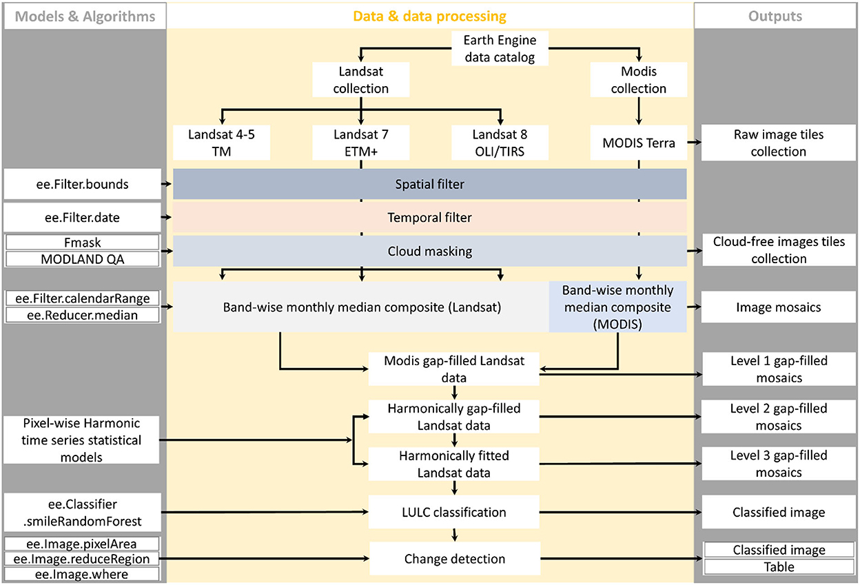
Figure 2. Image processing routine used for a spatial analysis of mangrove vegetation of The Gambia.

Image processing

As mentioned earlier, we used the geometrically and atmospherically corrected Landsat surface reflectance products. These products are provided along with a quality assessment band, which we used to mask all pixels affected by remote sensing artifacts (Figure 2). Although these are currently among the best available Landsat and MODIS products in the public domain, they often need to be further processed prior to analysis involving continuous observations. Since the atmospheric correction may fail to account for these remote sensing artifacts (Zhu and Woodcock, 2014), we discarded all pixels but those acquired under clear conditions (Figure 2). In the few cases where no clear acquisition is available, we created an empty image to keep track of missing data and provide a slot for gap filling, which we conducted in 3 steps. Roy et al. (2016) noted the differences between OLI and other Landsat data and provided coefficients for harmonizing these using linear transformations. We scaled all data from other sensors to OLI, so that the time series can be compared over the reference periods. This is particularly important for studies using water or vegetation indices because the difference is higher in the near-infrared and shortest wave infrared bands whereas atmospheric correction increases this difference in the visible bands (Roy et al., 2016).

The first step for gap filling consists in computing the monthly median composites, considering a lag of 31 days (Figure 2). This reduced the number of images to 12 median images per year, corresponding to 1 image per month. The median has proven to be a robust statistic in the sense that it is tolerant of outliers and noisy observations.

In the second step, we used the median of the corresponding MODIS acquisition of the month to fill data gaps in the Landsat composite where these MODIS data are available. We then computed the normalized difference spectral indices (i.e., NDVI, Gao NDWI, Mcfeeters NDWI, and EVI), which we used for subsequent analysis. The use of these indices can also improve the accuracy of data estimates since values beyond the range [−1, 1] are systematically discarded, even though EVI is not conceptually bounded by this value range. The choice of these 4 spectral indices is motivated by their sensitivity to water and vegetation, which are sufficient to describe the landscape of the study area when times series are available.

The third step relies on vegetation and water seasonality in the study region; hence, the temporal relationships between consecutive observations captured in the time series, to infer missing data using harmonic modeling (Figure 2). Many realistic models for time series analysis assume a component describing a consistent signal and another component representing random noise (Shumway and Stoffer, 2011). This is consistent with the behaviors of most ecological systems, particularly in the study area. We adopted the harmonic modeling approach to minimize the effects of such noise which are a mere representation of ephemeral variability. Under these considerations, we described pixel values as random variables chronologically indexed by time.

$\begin{array}{ll}Let\left\{p_t;t=t_0,t_1,\dots ,t_N\right\}& (1)\end{array}$

p_t is the predicted pixel value at time t

p_t = β₀ + β₁ t + e_t

Where,

β₀ is the intersept of the regression line

β₁ is the slope of the regression line

e_t is the random noise

p_t is the predicted pixel value at time t

Many problems in the frequency domain of time series analysis can be expressed as local, polynomials, and splines regression using linear models (Shumway and Stoffer, 2011). In the situation where the trend is of interest, the time series can be described using a linear regression model that predicts the pixel values based on time Equation (2).

$\begin{array}{c}\begin{array}{c}\hfill p_t = {\beta }_0 + {\beta }_{1}t + A\cos (2\pi \omega t+ \phi )+ e_t(Nonlinear form)\hfill \end{array}\\ \begin{array}{c}\hfill p_t = {\beta }_0 + {\beta }_{1}t + {\beta }_2\cos (2\pi \omega t) + {\beta }_3\sin (2\pi \omega t)+ e_t(Linearized form)\hfill \end{array}\end{array}(2)$

Where,

β₀ is the intersept (Starting point of p)

β₁ is the slope (How fast p changes with time)

t is the time indexed at t₀, t₁, …, t_N (Time since the epoch in radians)

A is the amplitude (The peak)

ω is the frequency of oscillation (ω = 1 for a single cycle)

φ is a phase shift (Time at which p reaches its peak)

β₁t is then, the linear term (Inter-annual variability)

A cos (2πωt+φ) is then, the harmonic term (Main signal as sinusoidal waveform)

e_t is the random noise

p_t is the predicted pixel value at time t

β₂, β₃ are the harmonic coefficients (Intra-annual variability)

With,

β₂ = A cos (φ)

β₃ = −A sin (φ)

$A={({\beta }_2^2+{\beta }_3^2)}^{1/2}$

$\phi =\left(\frac{{\beta }_3}{{\beta }_2}\right)$

$\begin{array}{ll}Acos(2\pi \omega t+\phi )={\beta }_{2}cos(2\pi \omega t)+{\beta }_{3}sin(2\pi \omega t)& (3)\end{array}$

In the situation where the periodic component is of interest, as is the case in our study region, linear regression can still accurately recover the periodic signal using sines and cosines as inputs (Shumway and Stoffer, 2011; Zhu and Woodcock, 2014). To accurately represent the prevailing seasonal variation in water and vegetation in the study region, we adopted a nonlinear model with a sinusoidal waveform [Equation (2); nonlinear form] which we linearized [Equation (2); linearized form] to fit local ordinary least squares regression (OLS) models that predict the values of NDVI, Gao NDWI, Mcfeeters NDWI, EVI, along with the green, the shortest wave infrared, and the thermal bands based on time. As earlier mentioned, the choice of the 4 spectral indices is motivated by their suitability to achieving the objectives of the study. We specifically included the 3 additional raw bands (i.e., the green band, the shortest wave infrared band, and the thermal band) in the harmonic modeling for later use in LULC classification (refer to section 2.4.2). For each pixel, we considered one cycle a year, corresponding to the single rainy season in the study area, to compute the OLS coefficients and fully specify the model which we then used to fill the remaining gaps in the original time series (Figure 3). We adopted the same harmonic modeling approach on the gap-free time series to remove random noise and recover the main signal which we used as input for subsequent analysis.

FIGURE 3

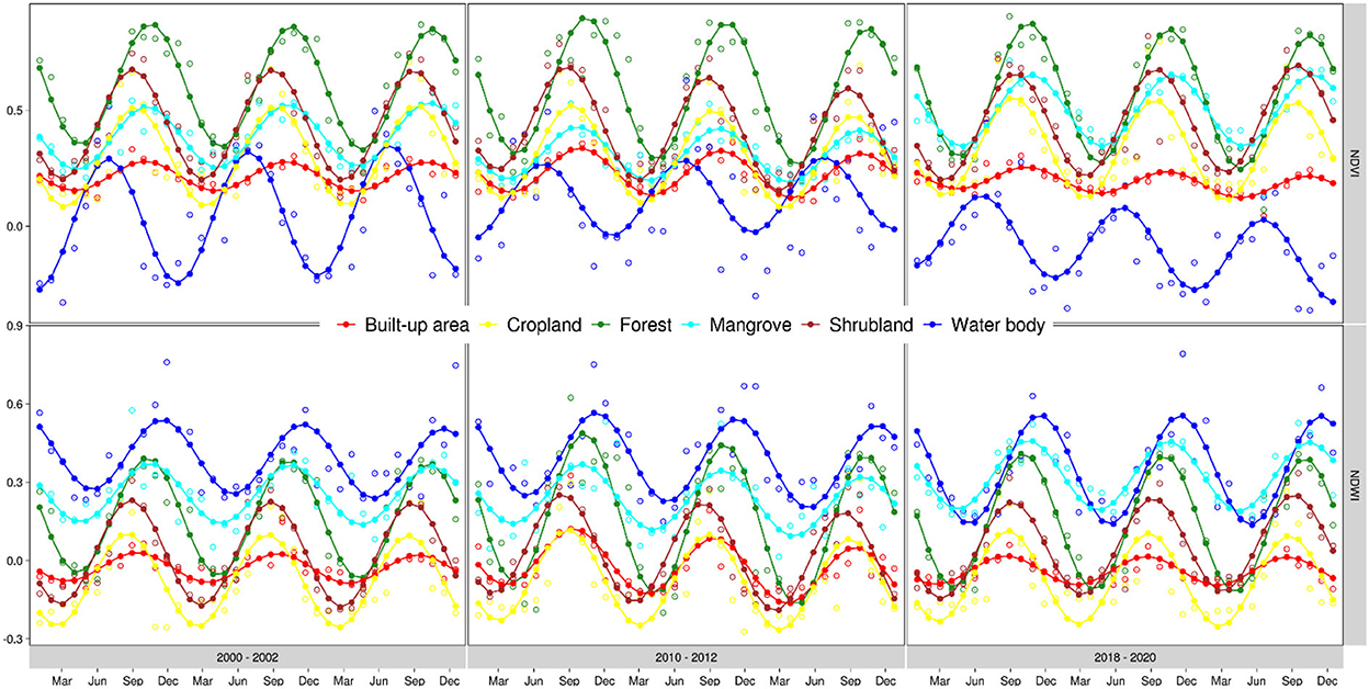
Figure 3. Available monthly median Landsat NDVI and Gao NDWI values after MODIS gap filling, and their corresponding gap-filled and predicted values estimated using harmonic modeling at a different location in The Gambia. This figure illustrates how the model fits different data inputs to capture the variations across multiple pixels. Non-solid circles represent the raw Landsat data after gap-filling using MODIS data. Dots (inside non-solid circles) represent gap-filled data after harmonic modeling. Solid circles are fitted values after harmonic modeling. Non-solid circles without a dot inside are noisy data detected and removed by the harmonic prior to computing the fitted values.

Land use and land cover classification and accuracy assessment

From the output of the model described in Equation (2), several components can be extracted and used in LULC classification. Herein, we used the predicted value, the estimated phase, and the estimated amplitude of the model. For each reference period, the fitted model outputs the 148 fitted bands corresponding to an image every month (30 days). Note that we only used the phase and the amplitude (not the fitted bands) for the green, the shortest wave infrared, and the thermal bands included while fitting the harmonic model (refer to section 2.4.1). With an amplitude and a phase for each of the 7 bands used in fitting the harmonic model (NDVI, Gao NDWI, Mcfeeters NDWI, EVI, green, shortest wave infrared, and thermal bands), the fitted model includes 14 additional bands summarizing the magnitude (peak) and the wavelength (spread) of the phenological cycle. We used the phase and amplitude of the green band because they provided us with a fairly good medium for distinguishing between areas where the 4 spectral indices are similar. In particular, the Gao and Mcfeeters NDWIs can often be very similar as is the case for NDVI and EVI. Therefore, the preprocessed data for image classification consisted of a large image of 162 (148 fitted bands + 7 phases + 7 amplitudes) bands for each reference period. To provide comprehensive accuracy assessments, we split the 16,000 reference data points collected into 70% for training and 30% for validation. For each reference period, we trained and validated a random forest classifier considering a maximum number of 100 trees. The accuracies of the 3 models are almost identical and we did not prefer one over another. Instead of using one of the 3 models in the supervised classifications, we classified the images of the 3 reference periods using their corresponding models. It is important to emphasize that classifications aiming to accurately detect LULC change, as in the case of change detection based on image comparison, should use classifiers that are comparable in regard to their throughputs, or at least a single model to ensure the comparability of the results.

Land use and land cover analysis

To provide a general picture of the landscape stability and disturbance, we examined the changes in all LULCs considered. We then provide a more detailed analysis specifically tailored to mangrove forests. These include the quantitative estimates of mangrove dynamics and change magnitude along with a qualitative analysis resulting in the mapping of change direction. In a nutshell, the analysis first involved the comparison of the 2000-classification against the 2020-classification to estimate LULC changes over the entire study period. We then compared the 2000-classification against the 2010-classification looking for a change that may have occurred during the decade 2000–2010 and the 2010-classification against the 2020-classification for change that may have happened during the decade 2010–2020. The analysis of LULC changes consisted in estimating the areas of the major LULC over time using simple GIS operation. We estimated the areas occupied by each LULC classes over time using the multitemporal classification. The changes over the entire study period [Change (2020–2000)] were estimated by subtracting the estimates based on 2000-classification from the ones based on the 2020-classification. The analysis of the mangrove dynamics and change magnitude consisted in examining the areas where mangrove changes have occurred using a simple classification comparison. We estimated the areas by comparing LULC over areas detected as mangroves during one or more of the reference periods considered. This results in a mangrove mask, which we used to mask all other areas and compute the share of mangrove losses and gains in relation to other LULCs. Mangrove change direction analysis consisted of grouping these areas into 3 categories including areas where mangroves were converted into other LULC (decrease), areas where mangroves remained (stable), and areas where other LULC became mangroves (increase).

Results

Accuracy assessment of land use and land cover classifications

The accuracy assessment shows that the random forest classifications have comparable accuracy, with an overall accuracy of 0.98 for the 2020-classification, 0.96 for the 2010-classification, and 0.97 for the 2000-classification. Similarly, the Kappa statistics are close enough to the overall accuracy to warrant the reliability of the classifications. We achieved a Kappa of 0.98 for the 2020-classification, a Kappa of 0.96 for the 2010-classification, and a Kappa of 0.96 for the 2000-classification (Table 2). The producer accuracy ranges from 0.92 to 1.00 for the 2020-classification, 0.87 to 1.00 for the 2010 classification, and 0.89 to 1.00 for the 2000-classification. The user's accuracy ranges from 0.92 to 1.00 for the 2020-classification, 0.87 and 1.00 for the 2010-classification, and 0.88 to 1.00 for the 2000-classification. Mangroves, for which all validation samples were correctly classified in the 2000-classification, are the classes with the best classification accuracy owing to a producer and user's accuracy between 0.99 and 1.00. With this level of accuracy, the 3 classifications can reliably serve the purpose of change detection.

TABLE 2

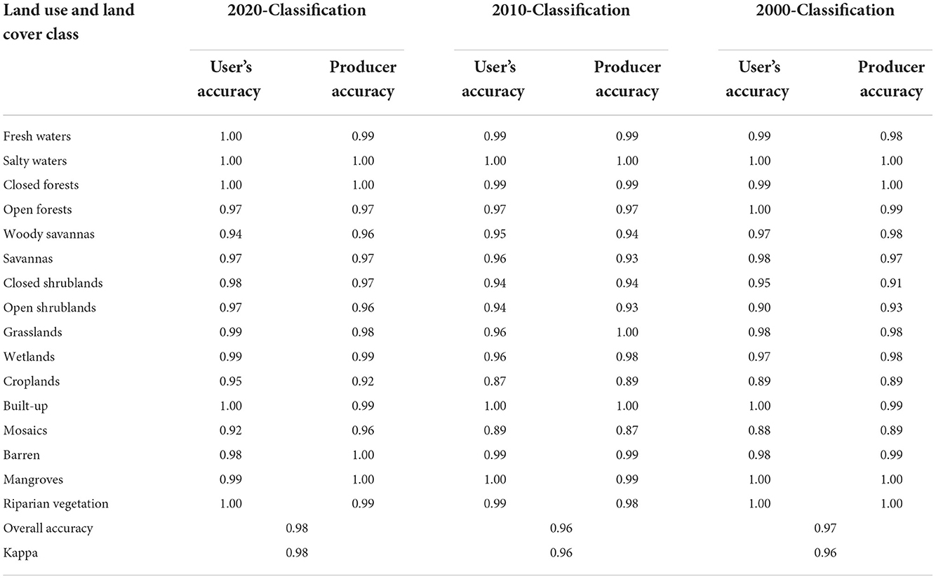
Table 2. Accuracy assessment of multi-temporal land use and landcover classifications used for assessing the dynamics of mangrove forests in The Gambia between the period 2000 and 2020.

Country-wide analysis

Dominant land use and land cover at a glance

While we identify 16 major LULCs in The Gambia, croplands, open and closed shrublands, woody savannas, savannas, and mangroves are the dominant ones from an aerial view of The Gambia (Figure 4).

FIGURE 4

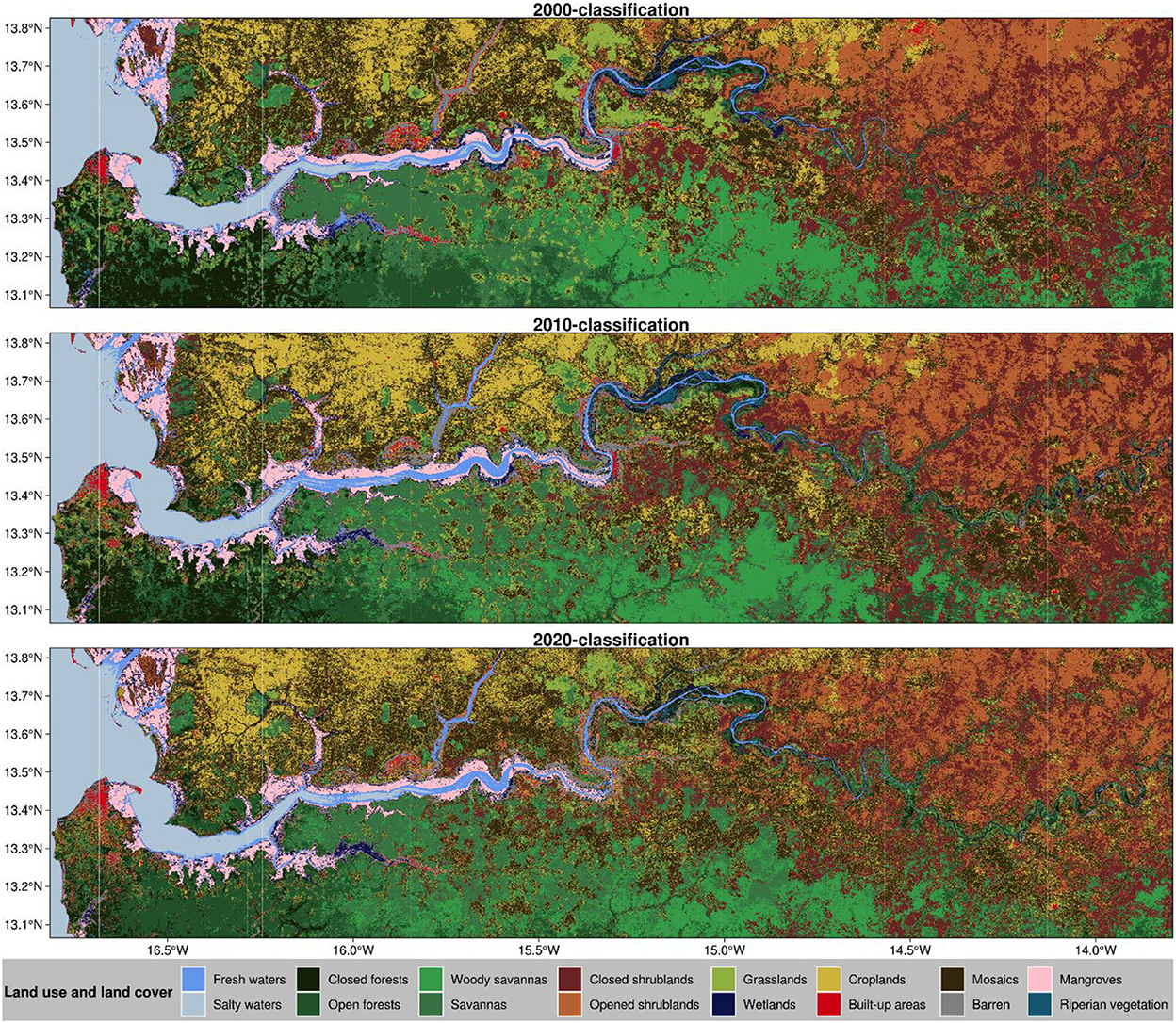
Figure 4. Land use and land cover classifications of The Gambia based on harmonic modeling of image time series acquired over the periods 2000–2002 (2000-classification), 2010–2012 (2010-classification), and 2018–2020 (2020-classification). These maps were derived by filling data gaps in Landsat monthly median composites using the equivalent MODIS data where these MODIS data are available.

Wetlands, riparian vegetation, closed forests, grasslands, and barren lands are less perceptible. Croplands and cropland/natural vegetation mosaics are mostly found in North Bank Region around Bao Bolong Wetland and Farafeni town toward the border with Senegal. Forests are mostly found in Western Region where open forests extend westwards toward the Bitang Bolon River into Senegal. Closed forests are limited to the coastal region following the coastline into Senegal. Western Region is the most populated region in The Gambia, with most of the build-up areas concentrated in the coastal part of the region, particularly in the greater Banjul showing a rapid urbanization sprawl. Savannas followed by woody savannas dominate the Lower River Region of The Gambia where croplands and cropland/natural vegetation mosaics occupy a substantial area. Mangroves, wetlands, and riparian vegetation are mainly found all over the bank of River Gambia from the Atlantic Ocean to the Upper River Region. These land covers are also found in most tributaries of River Gambia. The most developed mangroves of The Gambia are found in the Western Region, Northern Bank Region, and Lower River Region, particularly in Tanbi Wetland, Baobab Bolon Wetland, Mini Minium Bolon, Bitang Bolon River, and the upper part of Niumi National Park. Grasslands and cropland/natural vegetation mosaics cover most part of the Central River Region where we noticed a sizeable share of wetlands and bare lands toward the upper part of the region. Shrublands are mainly found in the Upper River Region with a southward increasing vegetation density. Closed shrublands are more visible in the southern part of River Gambia whereas open shrublands are more visible in the northern part of the river.

It appears that mangroves, open forests, woody savannas, and croplands have been steadily increasing over the last 2 decades. In contrast, closed forests, savannas, grasslands, and wetlands have been steadily decreasing. On the other hand, it appears that cropland/natural vegetation mosaics, closed shrublands, salty water, and built-up experienced an increase between 2010 and 2020 whereas they have seen a decrease between 2000 and 2010. Contrastingly, open shrublands, barren, fresh water, and riparian vegetation have seen a decrease between 2010 and 2020 whereas they have seen an increase between 2000 and 2010 (Table 3). From the analysis of the dynamics of the major LULC of The Gambia, we found out that some LULCs exhibit a gradual increase; others have fluctuating trends with both increase and decrease, and some others show a gradual decrease.

TABLE 3

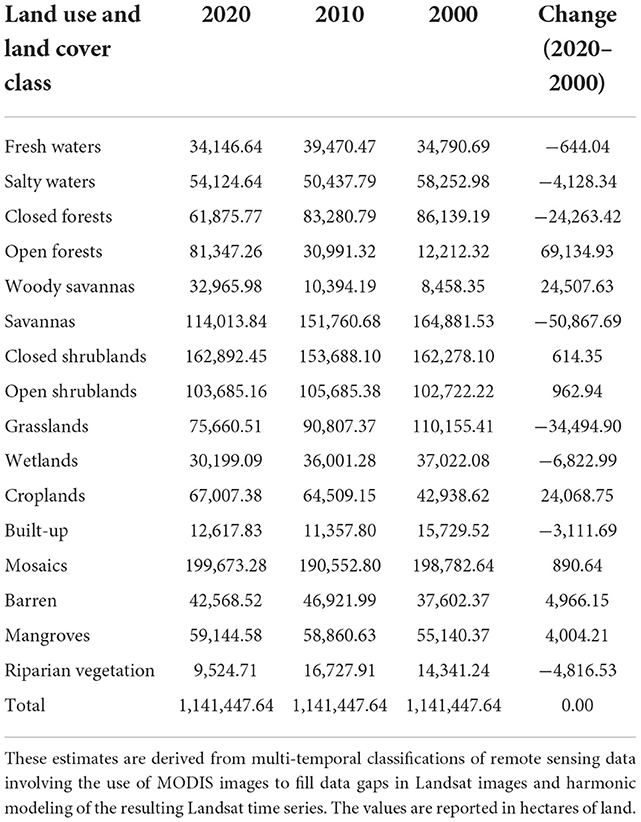
Table 3. Quantitative estimates of changes in major land use and land cover of The Gambia between 2000 and 2020.

Except for closed and open shrublands and mangroves, most LULC classes pertaining to the natural vegetation of The Gambia exhibit a declining trend over the 20-year study period. Natural vegetation (e.g., closed forests, savannas, grasslands, and wetlands) has been declining in favor of semi-natural vegetation (e.g., croplands and cropland/natural vegetation mosaics), sparse natural vegetation (e.g., closed shrublands, open shrublands), and even in favor of surface that is not favorable to vegetation (e.g., barren).

It is clear from our findings that several natural vegetation classes have been shrinking since 2000. The area closed forests occupy decreased from 86,139.19 ha in 2000 to 61,875.77 ha in 2020, resulting in a net loss of 24,263.42 ha. Savannas experienced a net reduction of 50,867.70 ha (i.e., from 164,881.50 ha in 2000 to 114,013.80 ha in 2020). Grasslands reduced gradually from 110,155.41 to 75,660.51 ha, making a net loss of about 34,494.90 ha. We estimated a net reduction of wetlands area of around 6,822.99 ha, owing to the drop from a total area of 37,022.08 ha in 2000 to 30,199.09 ha in 2020.

Despite the losses in some natural vegetation land covers, we observed substantial increases in other classes including mangroves, open forests, and woody savannas. Mangroves made an important gain with a total area of about 4,004.21 ha (i.e., from 55,140.37 ha in 2000 to 59,144.58 ha in 2020) over the 20-year period. Open forests increased from 12,212.32 ha in 2000 to 81,347.26 ha in 2020, making a total gain of 69,134.94 ha. Woody savannas also increased from 8,458.35 ha in 2000 to 32,965.98 ha in 2020, gaining a total area of 24,507.63 ha. Among the semi-natural vegetation, we estimated a gradual net increase in croplands of 24,068.76 ha (i.e., from 42,938.62 ha in 2000 to 67,007.38 ha in 2020).

Owing to the fluctuating trend across the 2 decades, our analysis remains unconclusive in regard to some classes of natural vegetation. We expect, however, that open shrublands have increased by 963.00 ha, and closed shrublands increased by 614.40 ha, whereas riparian vegetation decreased by 4,816.53 ha. We noticed the same fluctuating trend in non-vegetated classes such as barren for which we conjecture an increase of around 4,966.15 ha, fresh waters for which we look for a reduction of 644.05 ha, salty waters which we bet to have reduced by 4,128.34 ha, and built-up areas where we suspect a reduction of 3,111.69 ha. Among the semi-natural vegetation, cropland/natural vegetation mosaics also exhibit a fluctuating trend despite a total gain of 890.70 ha.

Mangrove change direction

From an aerial view of The Gambia, mangroves appear to have remained dominantly stable over the study period (Figure 5). Nevertheless, we noted a few spots of both increase and decrease spread across the country. It seems that the areas of increase dominate the areas of decrease. While The Gambian mangroves appear to do well over the study period, it would be important to have a closer look at these sites since such analysis can provide useful information for site-specific interventions.

FIGURE 5

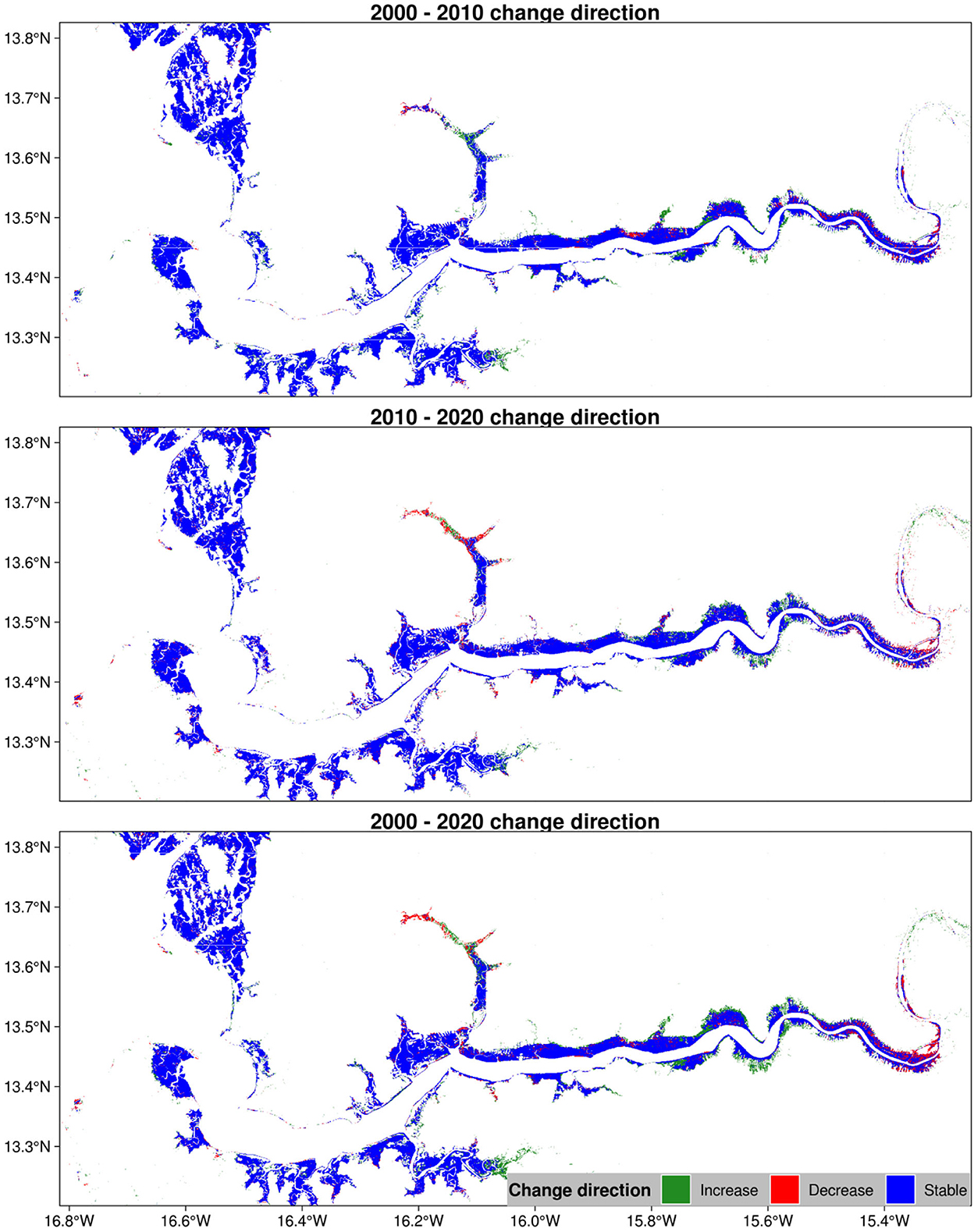
Figure 5. Change direction in mangrove vegetation cover of The Gambia based on harmonic modeling and classification of Landsat and MODIS time series. This figure was cut off to exclude empty space for better visualization.

In general, the stability is inclined toward an increase around the coastal regions whereas it tends toward a decrease near the Central River Region. We identified a few sites that have experienced an increase in mangrove forests as well as those that have seen a decrease in this vegetation over the study period. Sites of increasing trend can be found near Balingho, Bitang Bolon, and Darsilami. Those of decreasing trend are observed near Bambali Island and Mini Minium. We will look at these sites in more detail in the next sections.

Mangrove dynamics and change magnitude

Our results suggest that mangroves experienced a net gain of around 9,673.26 ha against a net loss of around 5,669.05 ha between 2000 and 2020. Most of the gain mangroves made came at the cost of riparian types of LULCs. Over the study period (2000–2020), mangroves gained about 5,263.35 ha of land at the expense of wetlands and around 3,146.91 ha against riparian vegetation. We observed relatively minor gains at the expense of woody savannas where mangroves gained around 1,680 ha and savannas where they gained an approximate area of 1,122 ha. Despite the net gain, mangrove forests experienced a sizeable shrink in many areas across The Gambia. Mangroves lost an approximate area of 2,213.04 ha in favor of wetlands, about 1,729.76 ha in favor of riparian vegetation, and around 1,309.45 ha for closed forests (Table 4).

TABLE 4

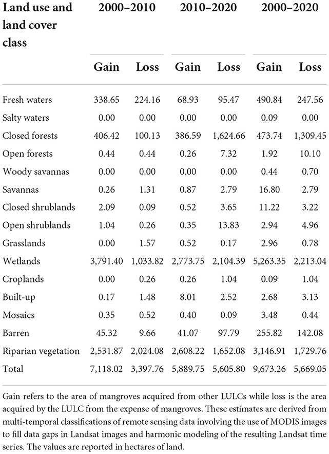
Table 4. Quantitative estimates of mangrove dynamics and changes magnitude in relation to major land use and land cover of The Gambia between 2000 and 2020.

During the decade 2000–2010, we estimated a total gain of 7,118.02 ha against a total loss of 3,397.76 ha. Wetlands contributed the most to these mangrove conversions during this decade. Wetlands lost around 3,791.40 ha to mangroves which lost around 1,033.82 ha to wetlands, corresponding to a difference of more than 2,500 ha in favor of mangroves (Table 4).

During the decade 2010–2020, we estimated a total mangrove gain of 5,889.75 ha, a gain that is slightly lower than the 7,118.02 ha estimated during the previous decade. In contrast, mangroves lost a slightly higher (5,605.08 ha) area than in the previous decade (3,397.76 ha). During this decade, mangrove gains came at the expense of wetlands (2,773.75 ha) and riparian vegetation (2,608.22 ha) whereas the loss is mainly due to the expansion of wetlands (2,104.39 ha), riparian vegetation (1,652.08 ha), and closed forests (1,624.66 ha) into mangrove areas (Table 4).

Site-specific analysis

Mangrove change direction

The site-specific analysis revealed greater insights in regard to the mangrove change direction. Mangroves have remained more or less stable in Tanbi Wetland (Figure 6) and Niumi National Reserve (Figure 7). Despite the general mangrove stability in these protected areas, we noted some spots of decrease in Crab Island and increase toward the north of Abuko Nature Reserve during the period 2010. Crap Island was once mangroves before 2000, and mangroves were converted into crab-breeding sites during the decade 2000–2010. During the same period, we note the degradation spots that have taken place inside Tanbi Wetland Reserve. It is interesting to investigate the cause and rate of this degradation.

FIGURE 6

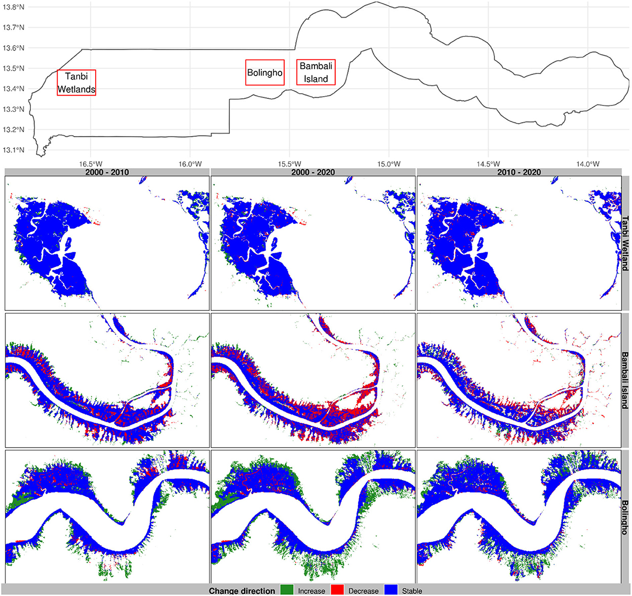
Figure 6. Change direction in selected mangrove sites of The Gambia based on harmonic modeling and classification of Landsat and MODIS time series. These maps are snapshots of Tanbi Wetland Reserve, Bambali Island, and Bolingho.

FIGURE 7

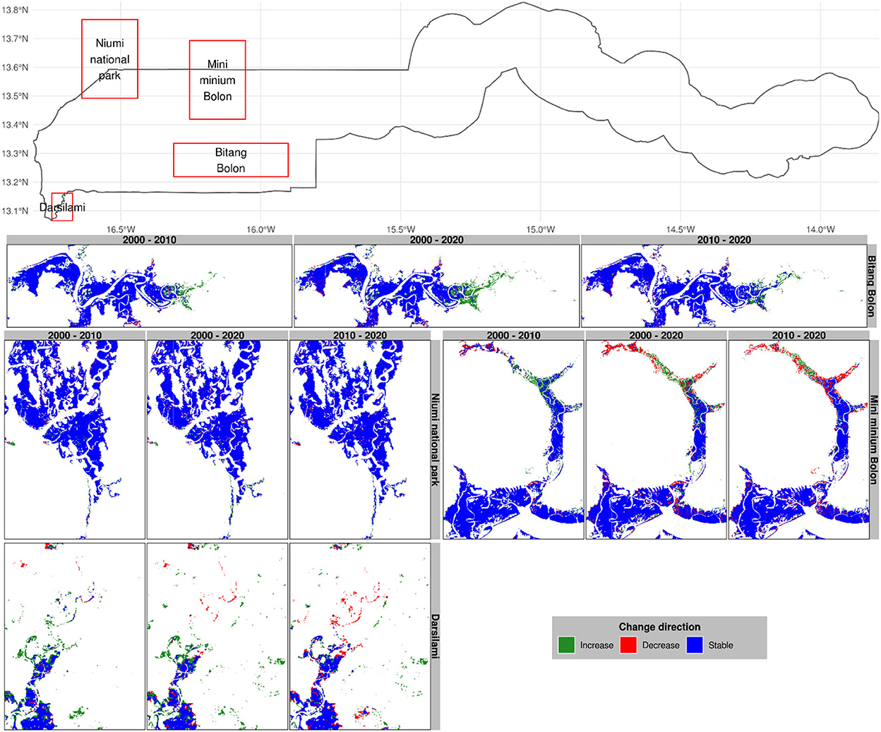
Figure 7. Change direction in selected mangrove sites of The Gambia based on harmonic modeling and classification of Landsat and MODIS time series. These maps are snapshots of Bitang Bolon, Mini Minium Bolon, Niumi national park, and Darsilami.

Mangroves appear to show a decreasing trend downstream near Bambali Island (Figure 6) and around Mini Minium (Figure 7) during the period 2010–2020. There is the general spread of mangrove degradation across the 2 decades in Bambali Island for which a substantial share of mangrove forests has been converted into other land covers. This is enough alarming to warrant immediate action because the mangrove ticket in this region is becoming narrower and tightened to the bank of the river that it is apparently heading toward complete degradation. We observed a similar trend of progressive degradation in Mini Minium Bolon where mangrove forests are progressively degrading from the head of the tributary to its mouth. Despite the substantial mangrove regeneration toward the head of the Mini Minium tributary, the degradation has alarmingly progressed during the last decade. We also noted an important degradation spot at the mouth where the Mini Minium tributary flows into River Gambia.

In Balingho (Figure 6), for instance, mangroves appear to be increasing since 2000. A similar pattern is observed in Bitang Bolon and Darsilami (Figure 7). Balingho presents an opposite trend compared to Bambali Island. Despite some patches of degradation in Balingho, mangroves have been progressively gaining land areas on either side of River Gambia. There is a general spread of mangroves onshore that has interestingly been taking place across the 2 decades. The mangrove ticket in this region is becoming wider around the river. Toward the head of Bitang Bolon, we noted an important increase in mangrove forests, despite a few spots of degradation in some of the tributaries of the river.

Mangrove change analysis

Mangrove forests have remained more or less stable in Tanbi Wetland and the vicinity of Niumi National Park toward the Senegal border (Figures 8, 9). Mangroves have substantially shrunk to riparian vegetation near Bambali island, constituting one of the major degradation hotspots in The Gambia (Figure 8). The area appears to be one of the most important mangrove disturbance sites in The Gambia. This area appears to show a pattern that suggests the conversion of mangrove forests into bare land. Essentially, mangroves become riparian vegetation during the decade 2000–2010, which riparian vegetation demote to shrublands during the following decade. Looking closely at the map, one can infer that the pattern of mangrove degradation in the Bambali region follows the following sequence: mangrove to wetlands, wetlands to riparian vegetation, and riparian vegetation to shrublands.

FIGURE 8

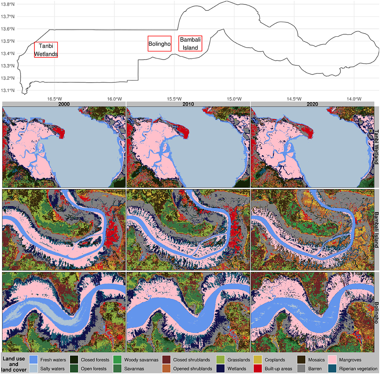
Figure 8. Land use and land cover classifications in selected mangrove sites of The Gambia based on harmonic modeling and classification of Landsat and MODIS time series. These maps are snapshots of Tanbi Wetland Reserve, Bambali Island, and Bolingho.

FIGURE 9

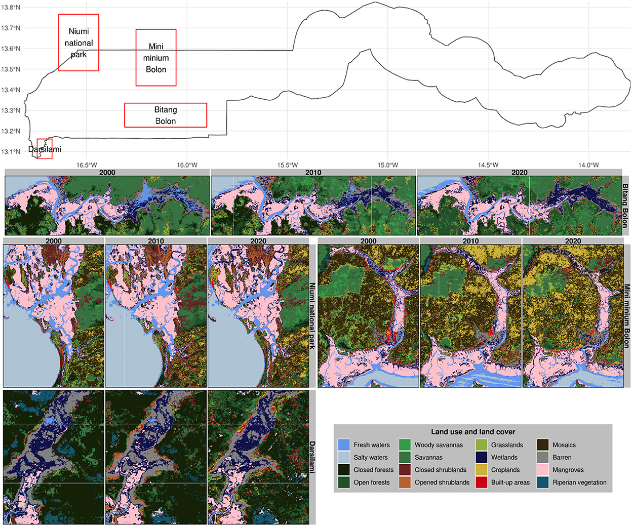
Figure 9. Land use and land cover classifications in selected mangrove sites of The Gambia based on harmonic modeling and classification of Landsat and MODIS time series. These maps are snapshots of Bitang Bolon, Mini Minium Bolon, Niumi national park, and Darsilami.

In the Bao Bolong River toward Katchang and near Balingho village where River Gambia meanders, mangrove forests appear to spread out off-shore on either side of the river, particularly in the lower part of the meander cut-off (Figure 8). Mangrove gain in this area seems to have occurred at the expense of wetlands and riparian vegetation. We also noted a widespread appearance of wetlands and riparian vegetation patches encroaching on mangrove forests. Our results suggest that mangroves have gained land area in this region but this expansion may have happened at a reduced vegetation density since the mangrove forests are becoming less compact. The area appears to exhibit a proliferation of riparian vegetation at the expense of mangroves and wetlands during the last decade. Overall, there seems to be an important reduction of bare lands in favor of vegetated lands in the region.

We noted a substantial increase in mangrove forests at the expense of wetlands and riparian vegetation in the Muni Munium River (Figure 9). Apparently, riparian vegetation nurtures wetlands, which later promote mangrove forests; a pattern that is nearly counterfactual to the one we observed in the Bambali region. In this region, we also noted an important mangrove degradation near Koular village where the mangrove downgraded to wetlands during the decade 2000–2010, which wetlands become closed forests during the following decade. The Bitang Bolon River region is characterized by a general increase in vegetation (Figure 9). Toward the outlet of the Bitang Bolon River tributary to River Gambia and around its sources near the border of the Lower River Region and West Coast Region, we noted an increase in mangrove forests at the expense of wetlands. In this region, fresh water appears to have become wetlands during the decade 2000–2010, and wetlands become mangroves during the following decade.

Discussion and conclusion

The declining trends in closed forests, savannas, grasslands, and wetlands have important implications for the rural population of The Gambia. This is quite crucial because these are LULCs that have a strong connection with the predominant pastoral and agropastoral livelihood of the majority of the community in The Gambia. A substantial share of these is lost in favor of mangrove vegetation. Although this gain in mangrove cover is a win for environmental conservation, we should not overlook its implication for the economy of The Gambia. Crow and Carney (2013) reported that increases in mangroves can mask the reduced ecosystem benefits gained by the locals from other LULCs. Future studies may assess the implications of mangrove gains on the livelihoods of the local community in The Gambia. The sequential pattern of mangrove conversion to shrublands through riparian vegetation in the Bambali Island region suggests a possible salinity drop or a drying trend in the region. The hypothesis of salinity is more plausible because the salinity generally decreases downstream, dropping below the tenth part per thousand in this region. The claim of the decreasing abundance of anadromous fishes in this region supports the explanation of decreasing salinity (Darboe, 2002; Albaret et al., 2004). This drop in salinity creates space for unfavorable mangrove conditions leading to their degradation, which contributes further to unfavorable habitats for these salty water fish species.

The conversion of mangroves into forests through wetlands in Muni Munium River suggests a limited reach of seawater that leads to decreasing water salinity such that the ecological conditions for mangrove forests are progressively degraded without significant effect on the overall moisture. This may explain the change of vegetation from mangroves to other types of vegetation beside the mangrove plant species. Due to the fertility of the area, this regular vegetation blooms to the extent that it masks the surface water beneath it when viewed from space.

The increase in non-mangrove forests in the Bitang Bolon River region suggests that the area experienced some drying that resulted in the regreening of waterways. This gave rise to the development of wetlands over minor rivers and streams and the conversion of some wetlands into riparian vegetation. The hypothesis of the drying is consistent with the claims of a prolonged dry period reported in The Gambia. The drying that occurred prior to the year 2000 led to an increased tidal reach of the seawater that has increased the general salinity along Bitang Bolon, causing important mangrove diebacks in the region (UNEP, 2007a; Fent et al., 2019). This conversion of wetlands into mangroves is the fruit of joint efforts and participative actions between several development agencies and the local population toward mangrove conservation. Between 2013 and 2014, the United Nations Development Programme (UNDP) initiated a widespread mangrove restoration project that brought together several other development institutions including Wetland International, the International Union for Conservation of Nature (IUCN), and the formation of the Sankandi Youth Development Association mandated at restoring the native mangrove forests. The Bintang Bolong River region shows several pockets of mangrove degradation before 2017. More than 3 ha of these have been restored in the vicinity of Bondali Tande village through the NEMA-CHOSSO project, a project supported by IFAD (International Fund for Agricultural Development). Since 2014, with the support of several development institutions (e.g., Earthwatch Europe, Reforestation World Switzerland, Network for Social Change), Sankandi Youth Development Association planted around 200,000 Red mangroves (Rhizophora mangle) along the Bintang Bolong riverbank.

The patches of the non-mangrove forests in the Balingho region suggest possible siltation of mangrove forests due to sediment deposition resulting from the river meandering. The presence of these patches may also indicate areas where mangrove replanting failed or mangrove seedlings (since there are currently ongoing mangrove planting activities in the region) that are too small to be detected from remote sensing. Since 2019, Community Action Platform on Environment and Development (CAPED) project has been restoring degraded mangrove forests across the entire Lower River Division. CAPED planted around 3 million mangrove saplings over an approximative area of 5 km along the Lower River, with the support of local communities and several government and non-government institutions. Between 2013 and 2018, UNDP supported a community development project that restored nearly 2,500 ha of mangrove forests along the Bao Bolong tributary near Darsilami and Illiassa villages and along the Bintang Bolong tributary near the Tendaba village.

The stability of mangrove forests in the Tanbi region is attributed to the protection of the area. Since 2007, the Tanbi Wetland complex enjoys a legally-binding protection status as a Ramsar site. In addition, the Tanbi region benefits from the support of several development institutions (e.g., WABSA—West Africa Study Birds Association, CONFORA—The Kombo/Foni Forestry Association) that guarantee its sustainable exploitation. Mangrove resources' usage in Tanbi Wetlands conveys certain norms of sustainable exploitation. A good example would be the Try Oyster Women's Association group that planted 6.7 ha with around 20,000 Rhizophora racemosa mangrove seedlings for a sustainable oyster collection.

The results of the dynamics of the major LULCs provide important insights for decision-making in regard to environmental planning because it provides key information on landscape disturbance. From these findings, decision-making has a clear guide for acting on biodiversity conservation. Knowing that some LULCs are shrinking, decision-makers can take action against the extension of a specific LULC depending on its importance for the local community. From our discussions on mangrove forest dynamics, it is clear that synergetic actions between community-based organizations and development agencies with clear goals have led to resilient mangrove forests in the Gambia. That is, strong governance and policymaking along with continuous environmental finance are the keys to sustainable management, but these may not be sufficient without proper incentives to embark on the locals and an adequate framework for managing the complex socio-institutional arrangements that are required at various scales.

Limitations of the study

The use of locally continuous time series along with the capability of the harmonic model to fill the data gap and remove noise in the temporal signature of LULC is essentially responsible for the high accuracy we have achieved in this study. The discontinuity of the time series outside the 3-year reference periods means that the predictions of the harmonic model are only based on the data corresponding to that temporal window. This means that the predictive power of the model can be improved using a longer period, preferably all available images. The longer the period, the more likely the number of clear pixels to infer the missing data and the more accurate the model predictions. One can then target the period of interest for LULC classification. An example of such algorithms is described in Zhu and Woodcock (2014) as continuous change detection and classification (CCDC). However, this entails the processing of a large amount of data, which can be challenging in terms of both acquisition and processing power among other requirements of the algorithm. This is particularly challenging for applications requiring high spatial resolution images. Switching to sentinel-2 data would result in at least twice the requirements in data storage and processing power compared to the Landsat data we used in this study.

Our findings are limited to the periods of interest (i.e., 2000, 2010, and 2020). The study remains inconclusive when it comes to what may have happened outside of these years. Further studies may look at the yearly dynamics of LULC along with the local perceptions of these changes. This would help to better explain the root causes of gains and losses (Fent et al., 2019). In fact, a lot can happen during the 3-year reference periods we have considered in this study. With the increasing data processing capability, it may be possible to generate an accurate land cover map from every gap-filled image and come up with some sort of probabilistic LULC assessment.

Our classifiers were able to separate salty and fresh water (Table 1, Figure 4). While discriminating fresh and salty water from multispectral images may seem far-fetched, the reaches of salty and fresh waters are visible on the ground that you attempted to show on the maps. Nevertheless, we currently do not understand this well enough to provide a detailed discussion, even though the distribution of mangrove tickets appears to be related to this gradient. Future studies may attempt to look at this phenomenon and its implication for mangrove vegetation.

Data availability statement

We conducted the data analysis in Google Earth engine cloud computing platform (Gorelick et al., 2017) and R programming language (R Core Team, 2021). These were interfaced using rgee R package (Aybar et al., 2020) which we used as bridge for throughput between Google Earth engine and R. Both Google Earth engine and R are freely accessible (see https://cran.r-project.org/index.html for R and https://code.earthengine.google.com/ for Google Earth Engine). We automated the entire process, including the installation of the required R packages, data processing, data streaming between Google Earth Engine and R, and result visualization, to provide a complete reproducible workflow. Replication files are available on Github at https://github.com/Issoufou-Liman/mangrove-frontiers.

Author contributions

PM, LD, and IL contributed to conception and design of the study. JI and IL organized the database, performed the statistical analysis, and wrote the first draft of the manuscript. IL, JI, and LD wrote sections of the manuscript. All authors contributed to manuscript revision, read, and approved the submitted version.

Funding

This research was supported by the American People through the United States Agency for International Development (USAID) under the BAA-AFR-SD-2020 Addendum 01, (FAA no. 7200AA20FA00031).

Conflict of interest

The authors declare that the research was conducted in the absence of any commercial or financial relationships that could be construed as a potential conflict of interest.

Publisher's note

All claims expressed in this article are solely those of the authors and do not necessarily represent those of their affiliated organizations, or those of the publisher, the editors and the reviewers. Any product that may be evaluated in this article, or claim that may be made by its manufacturer, is not guaranteed or endorsed by the publisher.

Author disclaimer

The contents of this manuscript are the sole responsibility of the authors and do not necessarily reflect the views of USAID or the United States Government.

Footnotes

1. ^According to certain definitions, degradation implies a reduction of certain properties of a LULC, but the LULC actually remains the same (e.g., forest degradation). In this paper, the term degradation refers to the complete conversion of one LULC to another.

References

Ajonina, G., Diamé, A., and Kairo, J. (2013). Current status and conservation of mangroves in Africa: an overview. J. Chem. Inform. Model. 53, 1689–1699.

Google Scholar

Albaret, J. J., Simier, M., Darboe, F. S., Ecoutin, J. M., and Raffray, J. (2004). Fish diversity and distribution in the Gambia Estuary, West Africa, in relation to environmental variables. Aquat. Living Resour. 17, 35–46. doi: 10.1051/alr:2004001

CrossRef Full Text | Google Scholar

Ali Bah, O. (2019). Land use and land cover dynamics in Central River Region of the Gambia, West Africa from 1984 to 2017. Am. J. Mod. Energ. 5, 1–5. doi: 10.11648/j.ajme.20190502.11

CrossRef Full Text | Google Scholar

Andrieu, J. (2018). Land cover changes on the West-African coastline from the Saloum Delta (Senegal) to Rio Geba (Guinea-Bissau) between 1979 and 2015. Eur. J. Remote Sens. 51, 314–325. doi: 10.1080/22797254.2018.1432295

CrossRef Full Text | Google Scholar

Aybar, C., Wu, Q., Bautista, L., Yali, R., and Barja, A. (2020). rgee: an R package for interacting with Google Earth Engine. J. Open Sour. Softw. 5, 2272. doi: 10.21105/joss.02272

CrossRef Full Text | Google Scholar

Ceesay, A., Dibi, H., Njie, E., Wolff, M., and Koné, T. (2017). Mangrove vegetation dynamics of the tanbi wetland national park in The Gambia. Environ. Ecol. Res. 5, 145–160. doi: 10.13189/eer.2017.050209

CrossRef Full Text | Google Scholar

Crow, B., and Carney, J. (2013). Commercializing nature: mangrove conservation and female oyster collectors in The Gambia. Antipode 45, 275–293. doi: 10.1111/j.1467-8330.2012.01015.x

CrossRef Full Text | Google Scholar

Darboe, F. S. (2002). Fish Species Abundance and Distribution in The Gambia Estuary. Tokyo: United Nations University. Available online at: https://www.grocentre.is/static/gro/publication/150/document/famara2002prf.pdf (accessed October 10, 2021).

Google Scholar

Di Gregorio, A. (2016). Land Cover Classification System: Classification Concepts, Software Version 3. Rome: FAO.

Google Scholar

FAO (2010). Country Profile: GAMBIA. Rome: FAO, 1–7.

Feka, Z. N., and Ajonina, G. N. (2011). Drivers causing decline of mangrove in West-Central Africa: a review. Int. J. Biodiver. Sci. Ecosyst. Serv. Manag. 7, 217–230. doi: 10.1080/21513732.2011.634436

CrossRef Full Text | Google Scholar

Fent, A., Bardou, R., Carney, J., and Cavanaugh, K. (2019). Transborder political ecology of mangroves in Senegal and The Gambia. Glob. Environ. Change 54, 214–226. doi: 10.1016/j.gloenvcha.2019.01.003

CrossRef Full Text | Google Scholar

FRA (2000). Forest Cover Mapping and Monitoring with NOAA: AVHRR and Other Coarse Spatial Resolution Sensors. Rome: FAO. Available online at: http://www.fao.org/forestry/4031-0b6287f13b0c2adb3352c5ded18e491fd.pdf (accessed October 23, 2021).

Gao, B. (1996). NDWI: a normalized difference water index for remote sensing of vegetation liquid water from space. Remote Sens. Environ. 58, 257–266. doi: 10.1016/S0034-4257(96)00067-3

CrossRef Full Text | Google Scholar

Gorelick, N., Hancher, M., Dixon, M., Ilyushchenko, S., Thau, D., and Moore, R. (2017). Google earth engine: planetary-scale geospatial analysis for everyone. Remote Sens. Environ. 202, 18–27. doi: 10.1016/j.rse.2017.06.031

CrossRef Full Text | Google Scholar

Jakubauskas, M., and Legates, D. R. (2000). “Harmonic analysis of time-series AVHRR NDVI data for characterizing U.S. Great Plains land use/land cover,” in International Archives of Photogrammetry and Remote Sensing (Amsterdam: International Society for Photogrammetry and Remote Sensing), 384–389. Available online at: https://www.isprs.org/proceedings/xxxiii/congress/part4/384_xxxiii-part4.pdf (accessed December 10, 2021).

Google Scholar

Liu, H. Q., and Huete, A. (1995). A feedback based modification of the NDVI to minimize canopy background and atmospheric noise. IEEE Trans. Geosci. Remote Sens. 33, 457–465. doi: 10.1109/TGRS.1995.8746027

CrossRef Full Text | Google Scholar

McFeeters, S. K. (1996). The use of the normalized difference water index (NDWI) in the delineation of open water features. Int. J. Remote Sens. 17, 1425–1432. doi: 10.1080/01431169608948714

CrossRef Full Text | Google Scholar

R Core Team (2021). R: A Language and Environment for Statistical Computing. Vienna: R Foundation for Statistical Computing. Available online at: http://www.r-project.org/ (accessed December 13, 2021).

Google Scholar

Roy, D. P., Kovalskyy, V., Zhang, H. K., Vermote, E. F., Yan, L., Kumar, S. S., et al. (2016). Characterization of Landsat-7 to Landsat-8 reflective wavelength and normalized difference vegetation index continuity. Remote Sens. Environ. 185, 57–70. doi: 10.1016/j.rse.2015.12.024

PubMed Abstract | CrossRef Full Text | Google Scholar

Satyanarayana, B., Bhanderi, P., Debry, M., Maniatis, D., Foré, F., Badgie, D., et al. (2012). A socio-ecological assessment aiming at improved forest resource management and sustainable ecotourism development in the mangroves of Tanbi Wetland National Park, the Gambia, West Africa. Ambio 41, 513–526. doi: 10.1007/s13280-012-0248-7

PubMed Abstract | CrossRef Full Text | Google Scholar

Shumway, R. H., and Stoffer, D. S. (2011). Time Series Analysis and Its Applications, 3rd Edn. New York, NY: Springer. doi: 10.1007/978-1-4419-7865-3

CrossRef Full Text | Google Scholar

Spalding, M., Blasco, F., and Field, C. (1997). World Mangrove Atlas, World Mangrove Atlas. Okinawa: The International Society for Mangrove Ecosystems.

PubMed Abstract | Google Scholar

The Gambia Bureau of Statistics (2013). The Gambia 2013 Population and Housing Census Preliminary Results. Serrekunda: The Gambia Bureau of Statistics.

Google Scholar

Tucker, C. J. (1979). Red and photographic infrared linear combinations for monitoring vegetation. Remote Sens. Environ. 8, 127–150. doi: 10.1016/0034-4257(79)90013-0

CrossRef Full Text | Google Scholar

UNEP (2007a). Mangroves of Western and Central Africa. UNEP Regional Seas Programme/UNEP-WCMC. Cambridge: UNEP.

Google Scholar

UNEP (2007b). Mangroves of Western and Central Africa. Cambridge: UNEP-WCMC, UNEP. Available online at: https://archive.org/download/mangrovesofweste07corc/mangrovesofweste07corc.pdf (accessed November 12, 2021).

Google Scholar

Vermote, E. (2015). MOD09A1 MODIS/Terra Surface Reflectance 8-Day L3 Global 500m SIN Grid V006 [Data Set]. Sioux Falls, SD: NASA EOSDIS Land Processes DAAC.

Wulder, M. A., Loveland, T. R., Roy, D. P., Crawford, C. J., Masek, J. G., Woodcock, C. E., et al. (2019). Current status of Landsat program, science, and applications. Remote Sens. Environ. 225, 127–147. doi: 10.1016/j.rse.2019.02.015

CrossRef Full Text | Google Scholar

Zhu, Z., Wang, S., and Woodcock, C. E. (2015). Improvement and expansion of the Fmask algorithm: cloud, cloud shadow, and snow detection for Landsats 4–7, 8, and Sentinel 2 images. Remote Sens. Environ. 159, 269–277. doi: 10.1016/j.rse.2014.12.014

CrossRef Full Text | Google Scholar

Zhu, Z., and Woodcock, C. E. (2014). Continuous change detection and classification of land cover using all available Landsat data. Remote Sens. Environ. 144, 152–171. doi: 10.1016/j.rse.2014.01.011

CrossRef Full Text | Google Scholar