Forest protection and permanence of reduced emissions

Tropical forests are essential for climate change mitigation. With growing interest over the use of credits from reducing emissions from deforestation and forest degradation (REDD+) and other natural climate solutions within both voluntary and compliance carbon markets, key concerns about the long-term durability of the reductions, or their permanence, arise for countries, corporations, regulators, and policy makers. This paper seeks to analyze the longevity of emissions reductions from different policies to slow down and stop deforestation. To establish conditions of permanence, we conduct numerical analyses using a model based on a cellular automata algorithm that learns from historical deforestation patterns and other spatial features in the Brazilian state of Mato Grosso. First, we simulate increased law enforcement to curb deforestation at a jurisdictional scale from 2025 to 2034, followed by potential policy rollbacks from 2035 to 2050. Second, we consider alternative scenarios to avoid potentially legal deforestation coupled with reforestation. We find spatial and path dependence – a successful policy intervention may permanently change the deforestation trajectory even after potential policy reversals. Hence, permanence depends both on the probability of policy reversals and the risk of emissions overshooting. Our results are important for advancing the understanding around the unsettled debate on the permanence of avoided emissions. Further, this paper argues that as policies to prevent deforestation or reduce emissions otherwise are reversible, permanence should be understood and discussed in a probabilistic and time-dependent framework.

Introduction

Deforestation accounts for roughly 14% of annual global greenhouse gas emissions (Harris et al., 2021) and reducing it is essential to any climate change mitigation strategy. Reducing emissions from deforestation and forest degradation plus the sustainable management of forests and the conservation and enhancement of forest carbon stocks is integral to climate change mitigation worldwide (REDD+).

Fuss et al. (2021) demonstrate significant macroeconomic value of REDD+ at the global level under a policy to stabilize emissions in line with the targets of the Paris Agreement. Their study forecast REDD+ could save “up to 22% of the cost of the global climate policy, generating $30.6 to $36.4 trillion in risk-adjusted cost savings.” There are also significant ancillary benefits of avoiding deforestation, but all of that could be gained only if the reduction of emissions is “permanent.”

In order to materialize REDD+ gains, it is important to understand the driving forces behind deforestation. Many studies distinguish between proximate/direct causes and underlying/indirect causes of deforestation and forest degradation (e.g., Geist and Lambin, 2002; Kissinger et al., 2012). Proximate causes are those resulting from human activity, such as agricultural expansion or livestock grazing, while underlying causes arise from the social, economic, and political systems at work.

Many studies have identified a variety of proximate agents of deforestation and forest degradation. These include livestock production (Müller-Hansen et al., 2019), agricultural expansion (Barbier, 2004; Acheampong et al., 2019), logging (Bowles et al., 1998; Islam and Sato, 2012), mining (Sonter et al., 2017), hydroelectric dams (Chen et al., 2015), and property rights (Mendelsohn, 1994).

Each of these drivers can directly impact deforestation rates. They are easily identifiable and can thus be controlled more readily than some of the broader underlying institutional or economic drivers of deforestation. For instance, Tumusiime et al. (2018) found that institutional drivers of deforestation in Uganda included “budgetary constraints, corruption, the frequent trading of forests for political capital, and the unfettered growth in the number of districts (stretching already tight resources).” Certain studies have explicitly conceded that while institutional factors are important, their actual influence is difficult to quantify (Meyer et al., 2003).

Another important aspect of forest conservation strategies is ensuring that the mitigation attributed to avoided deforestation is “permanent.” The emissions reductions from an avoided deforestation project may not be “permanent” if those reductions are exposed to certain risk factors. Risk factors can be internal or external to the emissions reductions project (Verified Carbon Standard, 2011). If these risk factors are realized, the mitigation can be reversed, thereby offering only a temporary climate benefit. Such a reversal makes the emissions reductions associated with the project “non-permanent” as they do not exist in perpetuity. Since it is virtually impossible to guarantee the perpetuity of emissions reductions, most jurisdictional or project-based crediting programs designate a specific time period for which the avoided emissions must be maintained in order to be considered permanent (e.g., 40 years, 100 years, etc.).

Internal project risks are inherent to project design and management (Verified Carbon Standard, 2011). These types of risks can be related to project management or financial viability. They can also result from opportunity cost, in which there is a profitable alternative land-use activity where the avoided deforestation project is located. External project risks parallel those underlying risks discussed above. They are externalities outside the control of the project designer or manager, and can take the form of a lack of community engagement or a predisposition to natural disasters, such as wildfires.

With so many drivers of deforestation and risks of non-permanence, it is essential that governments design effective policies to both combat deforestation and ensure avoided deforestation permanence. Policies are effective in ensuring the permanence of avoided deforestation if they are continually enforced. To envision the effectiveness or lack thereof of a policy, we imagine alternative emissions pathways after the implementation and subsequent rollback of a given policy (see Schwartzman et al., 2021, Figure 1, p. 3). At time T₀, the policy is implemented and emissions from deforestation begin to decline. However, after some time the policy is rolled back, at which point we can envision four distinct potential paths with varying associated emissions. Path 1 sees deforestation and its associated emissions continue to decline. Path 2 sees emissions rise slightly but remain below the business as usual (BAU) trajectory pre-policy intervention. In Path 3, emissions return to the BAU trajectory. Finally, in Path 4 emissions exceed the BAU trajectory, with more emissions over time than in the absence of the policy. These four pathways allow us to examine the cumulative emissions associated with each counterfactual scenario following the rollback of a policy.

FIGURE 1

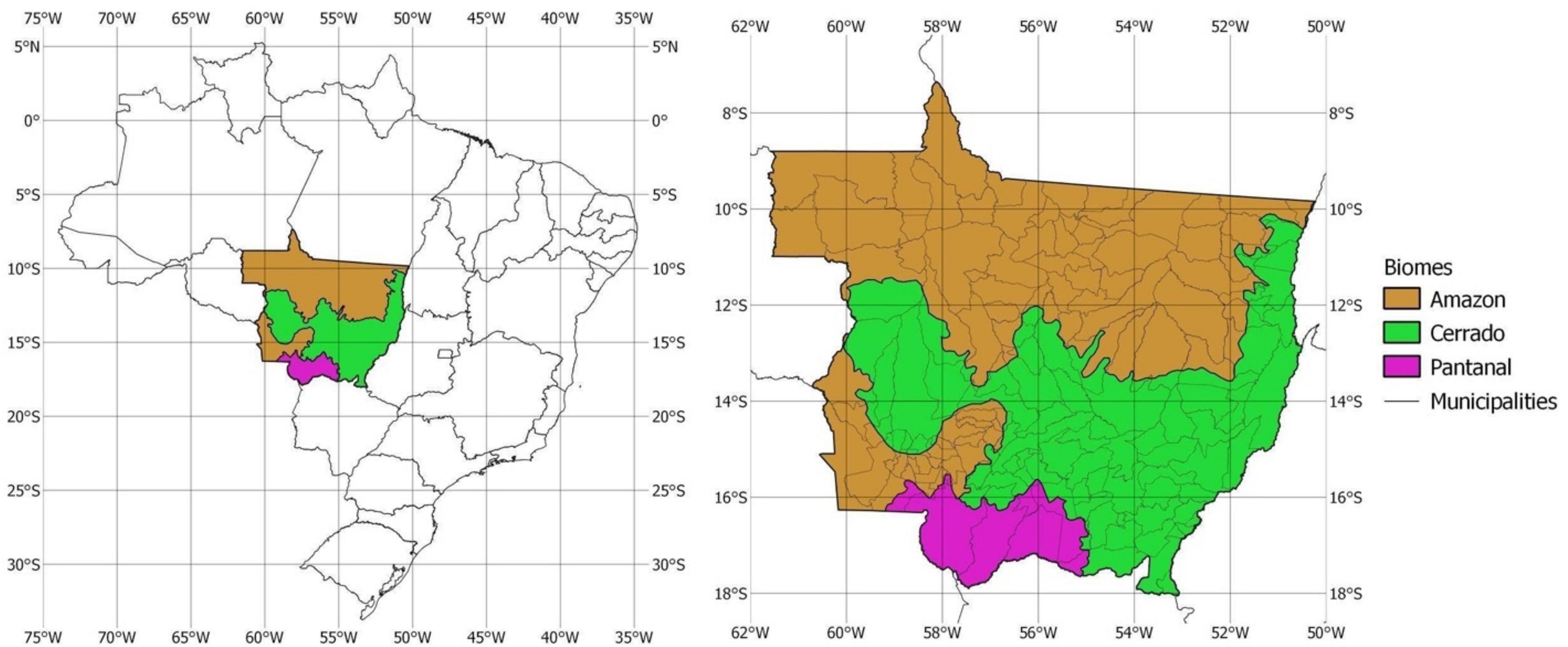
Figure 1. Study area: Mato Grosso and its biomes.

For numerical analysis we calibrate the model using data from the state of Mato Grosso, Brazil. For the permanence analysis we consider two (carrots-and-sticks) jurisdictional policies. The first simulates a jurisdictional command-and-control effort (sticks) to reduce deforestation in private and public lands. The second simulates a combination of return to compliance with the 2012 Brazilian Forest Code — i.e., reforestation of all areas within private properties with native vegetation deficits (sticks) coupled with an incentive mechanism (carrots) to avoid legal deforestation in properties with native vegetation surplus - i.e., beyond the Forest Code legal requirements. Both policies are aimed at generating REDD+ credits with a time horizon out to 2050.

This paper seeks to analyze different conservation policies to slow down and stop deforestation and explore the longevity/permanence of associated emissions reductions via modeling. We use deforestation data for the state of Mato Grosso, Brazil from 2001 to 2016, while controlling for covariates that affect forest clearings —including roads, conservation units and Indigenous lands, among others, to calibrate our model and the algorithm it uses to replicate historical deforestation. Further, we introduce mechanisms to break trends of historical deforestation and project the aforementioned scenarios. Our model investigates the spatial dependence of deforestation, or how deforested cells impact the behavior of their neighbors. Moreover, the model evaluates spatial correlation to probe for a possible unobserved factor that varies spatially, making it more likely that neighboring cells become deforested. We model increased law enforcement to curb deforestation at a jurisdictional scale to generate REDD+ credits from 2025 to 2034. From 2035 onward we simulate different scenarios to better understand how potential policy rollbacks would affect permanence of reduced deforestation and emissions. We simulate a continuation of tight law enforcement and different levels of law enforcement loosening by changing the threshold cutoff probabilities at which forestlands are cleared. However, results are applicable to any jurisdictional policy that is limited in time.

The paper is organized as follows. Section “Methodology” details the machine learning and cellular automata methodology employed. Section “Modeling approach” describes how we applied the cellular automata algorithm to learn from past deforestation patterns and other spatial features (e.g., indigenous lands), datasets employed, how the model was trained and calibrated, and how simulations were performed. Section “Results” presents the simulation results. In section “Discussion and conclusion,” we discuss our main conclusions and, in section “Future research,” we discuss future research possibilities.

Methodology

Our goal is to develop a simulation model of deforestation across a landscape that takes into account spatial interactions. The method we use is a particular form of cellular automata (CA). These are spatially and temporally discrete computational systems composed of cells, which evolve in parallel at time steps following dynamic transition rules: the update of a cell state depends on the states of cells in its local neighborhood.

Cellular automata is widely used for modeling spatial dynamics, including interactions between neighboring cells. Applications include modeling wildfire spread (Trucchia et al., 2019), propagation of epidemics (Sirakoulis et al., 2000), land-cover change and deforestation (Soares-Filho et al., 2002), and surface water flow (Parsons and Fonstad, 2007).

Cellular automata can be continuous or discrete. For example, Soares-Filho et al. (2002) uses continuous CA to model the transition of spatial probabilities of deforestation in the Amazon based on detailed input datasets, including information on various land-cover classes. Discrete CA has been used for modeling wildfire spread dynamics (e.g., Trucchia et al., 2019).

In CA, each cell can represent the state of several variables, which in turn interact with one another and are simultaneously subject to the states of other cells. Interaction between cells can be approached in several ways, including implementation of kernels and linear and non-linear functions. For instance, in modeling epidemic propagation (Sirakoulis et al., 2000) each cell represents a fraction of the total population in one of three states: infected, immunized, and susceptible.

In our approach, we use ideas of CA combined with the 2D convolution procedure and machine learning method. Specifically, we introduce a regression model in which neighborhood dynamics are included as a feature for model training. In addition, we define the state of each cell as probabilities (i.e., values between 0 and 1) of deforestation. Moreover, we modify the uniform influence of deforestation in neighboring cells by weighting their impacts. The weights are estimated using stationary features of neighboring cells. This is achieved by the 2D convolution operation (see, e.g., Zhang, 2019) proposed in this study. In that way, we tailor CA for our specific modeling purposes. We did not find this particular formulation of CA in the literature. Further, we find an advantage of our approach in that it captures the main features of the model while allowing for acceptable computational time.

Modeling approach

We employ a spatially explicit model of the evolution of deforestation probabilities, considering the following:

• Local drivers of deforestation.

• Impact of ongoing deforestation in neighboring cells.

• Cells where deforestation is made impossible.

• Policy scenarios based on centralized and local thresholds for deforestation.

• Random deforestation events (e.g., fires).

Our main hypothesis is that deforestation dynamics are driven by the relationships between deforested cells and cells that are not deforested. The assumption here is that deforestation is driven by deforestation itself, as it facilitates access to new sites. Thus, forested areas in the neighborhood of deforested cells have a higher chance of undergoing deforestation. In addition, there are local drivers of deforestation that increase its probability depending on the proximity of the area to roads, rivers and socioeconomic and other factors characterizing the area. Therefore, the probability of deforestation is predicated on interactions between two main components: (1) the current and historical status and probabilities of deforestation in the neighborhood; and (2) local drivers of deforestation. Once we assess the probability of deforestation of each cell, we can simulate the event of deforestation that is determined by a threshold value (in terms of probability). Then, we consider threshold values as policy variables, allowing us to model various scenarios of future deforestation depending on different threshold values set for the entire study area or its local subareas. Random deforestation events are considered by introducing the Monte Carlo scheme to generate probabilistic thresholds.

In this section, we describe the dataset employed, the algorithms and model assumptions. The structure of this section is as follows. First, we describe the study area, the dataset, and preprocessing. Second, we include the main parameters of the algorithm. Third, we provide details about model training. Finally, we describe assumptions for simulating scenarios.

Study area and time horizon

We consider the Brazilian state of Mato Grosso, located in the center of Brazil, for our analyses. Figure 1 shows the location of Mato Grosso in Brazil, as well as a detailed state map and its biomes.

Technically, the area consists of 1,298 × 1,194 grid cells, where each grid covers 1 km². Our sample uses deforestation data from the Secretary of Environment of the state of Mato Grosso (SEMA-MT) from 2001 to 2016. These data are used for model training using the approach described below. We use the 2010–2019 time period for model warm-up, and the 2020–2050 time period for future projections.

Mato Grosso has an area of 90.3 million ha, equivalent to the combined areas of France and Germany. In 2017, 53.5 million ha were covered by native vegetation, spanning three biomes — equivalent to approximately 59% of the state, or an area larger than Spain. Mato Grosso was able to reduce deforestation from 1.278 million ha in 2004 to 0.155 million ha in 2010, a drop of more than 85% in deforestation over 6 years across all biomes. It is also an agricultural powerhouse, being the top producer of a handful of agricultural commodities in the country. What’s more, from 2006 to 2017, the state was responsible for the bulk of deforestation reductions in Brazil, or 40,938 km² out of 62,321 km² (West et al., 2019). In the meantime, both soybean production and heads of cattle increased in the state. In addition, Mato Grosso is home to 125,000 smallholder farmers and 43 Indigenous ethnicities spread across 79 indigenous lands (International Policy Centre for Inclusive Growth et al., 2019).

For these reasons we chose the state as our area of study, as it is a crucial region for understanding the permanence of deforestation reduction policies in the presence of large agricultural production and Indigenous lands.

Data and preprocessing

In Table 1, we list the variables used in our model, including their name, description and type. Our outcome variable is yearly deforestation in Mato Grosso. In our model, past deforestation reinforces future deforestation. Other variables control for the spatial patterns of deforestation.

TABLE 1

Table 1. Features and variables used in the model.

First, we account for the state and municipal political boundaries. We then assign each pixel to an ecological zone according to the state’s biomes to account for different regulations in the 2012 Brazilian Forest Code. Part of the forestland in Mato Grosso is located in private rural properties, which are mandated to preserve 80% of their native vegetation in the Amazon (forest), 35% in the Cerrado (savanna), and 20% in the Pantanal (wetland). We include protected areas (i.e., conservation units and indigenous lands) where deforestation is unlawful. These act as strong, although not perfect, barriers against deforestation. Rural settlements are also included and have been identified as hotspots of deforestation (Assunção and Rocha, 2016).

Decay of deforestation events

In the historical data, the target variable — deforestation¹ — is represented by binary variables, indicating the year in which the deforestation occurred. We also assume that once a cell is deforested it stays that way forever. However, if we kept that assumption, deforested cells would stay at a value of 1 in all years of simulation runs, which would make it hard to distinguish their influence over time. As our model deals with the influence of neighbors and probabilities (values between 0 and 1), we propose the following transformation of binary values to take into account dynamic effects of deforestation.

Our decay approach reduces historical deforestation impacts based on the idea that deforestation that happened farther back in time has less impact compared to the most recent deforestation events (Fearnside, 1982). Consider that deforestation in pixel (i,j),i = 1,..,Q,j = 1,..,P, took place n years ago. Here, Q and P are the number of rows and columns, respectively, of a matrix corresponding to the study area map. At current time, t, we decay deforestation events in each pixel according to the equation:

$d_{ij}\left(t\right)={\mathrm{\delta }}^n{d}_{ij}\left(t-n\right),d_{ij}\in [0,1],t\in [t_0,T],n\in [0,t-t_0](1)$

Where δ is the decay factor. We set the decay factor to δ = 0.85². The corresponding matrix of decayed deforestation at time t is denoted by D(t) = (d_ij(t)) ∈ [0,1]^{Q × P}.

Application of decay to the deforestation data is illustrated in Figure 2. The earliest information about deforestation dates back to 2000, therefore in this year all pixels deforested as of that date have values equal to 1. After 5 years, those pixels deforested in 2000 decay and their values equal 0.44 (colored yellow in the figure) in 2005. At the same time, more recent deforestation events have happened and are happening in 2005, and the values at these locations are higher (orange and red colors). In 2010, pixels deforested in 2000 decay to 0.197 (colored lavender) and pixels deforested in 2005 decay to 0.44 (colored yellow).

FIGURE 2

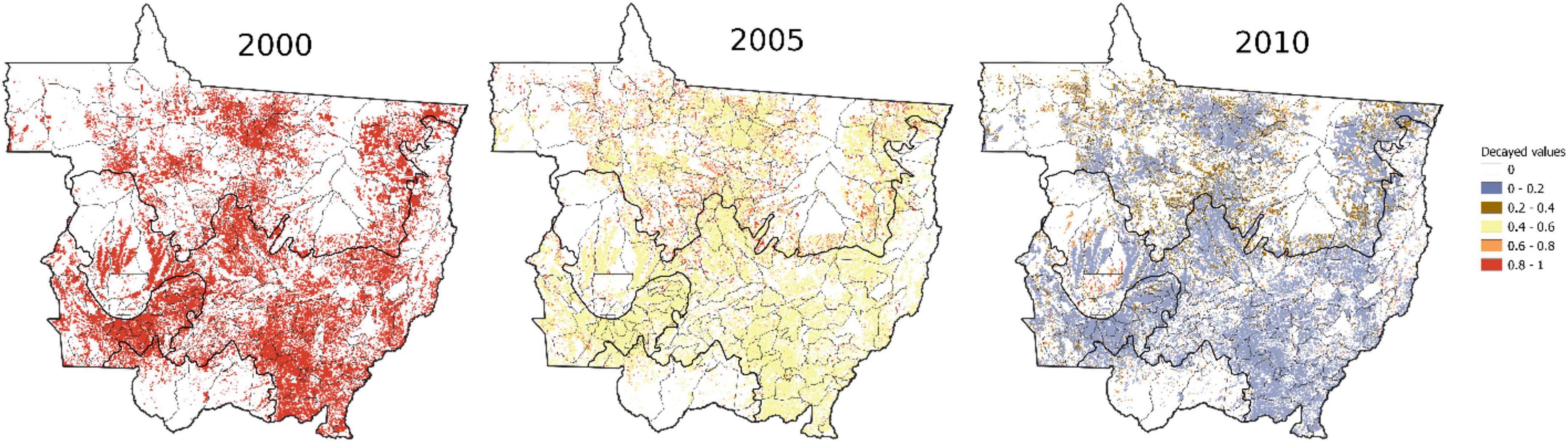
Figure 2. Decayed deforestation in relation to the year 2000, with a decay factor of δ= 0.85.

Model training

For model training, we apply a method based on gradient boosting from machine learning techniques. The scheme of feature collection is shown in Figure 3. We use stationary data from Table 1 and combine it with deforestation dynamics in the neighborhood to predict the target variable. The target variable is decayed deforestation, as explained in the preceding section, represented by a value between 0 and 1. The reason for predicting decayed values is because this is the only target the model “knows.” A lower value means that deforestation could potentially have happened long ago, while a higher value indicates that deforestation might have happened recently. As deforestation has not yet happened, the latter indicates the higher probability that it will. Thus, the “time” is reflected in the model when we predict when future deforestation will take place — i.e., the higher the predicted decayed value, the sooner deforestation is likely to happen.

FIGURE 3

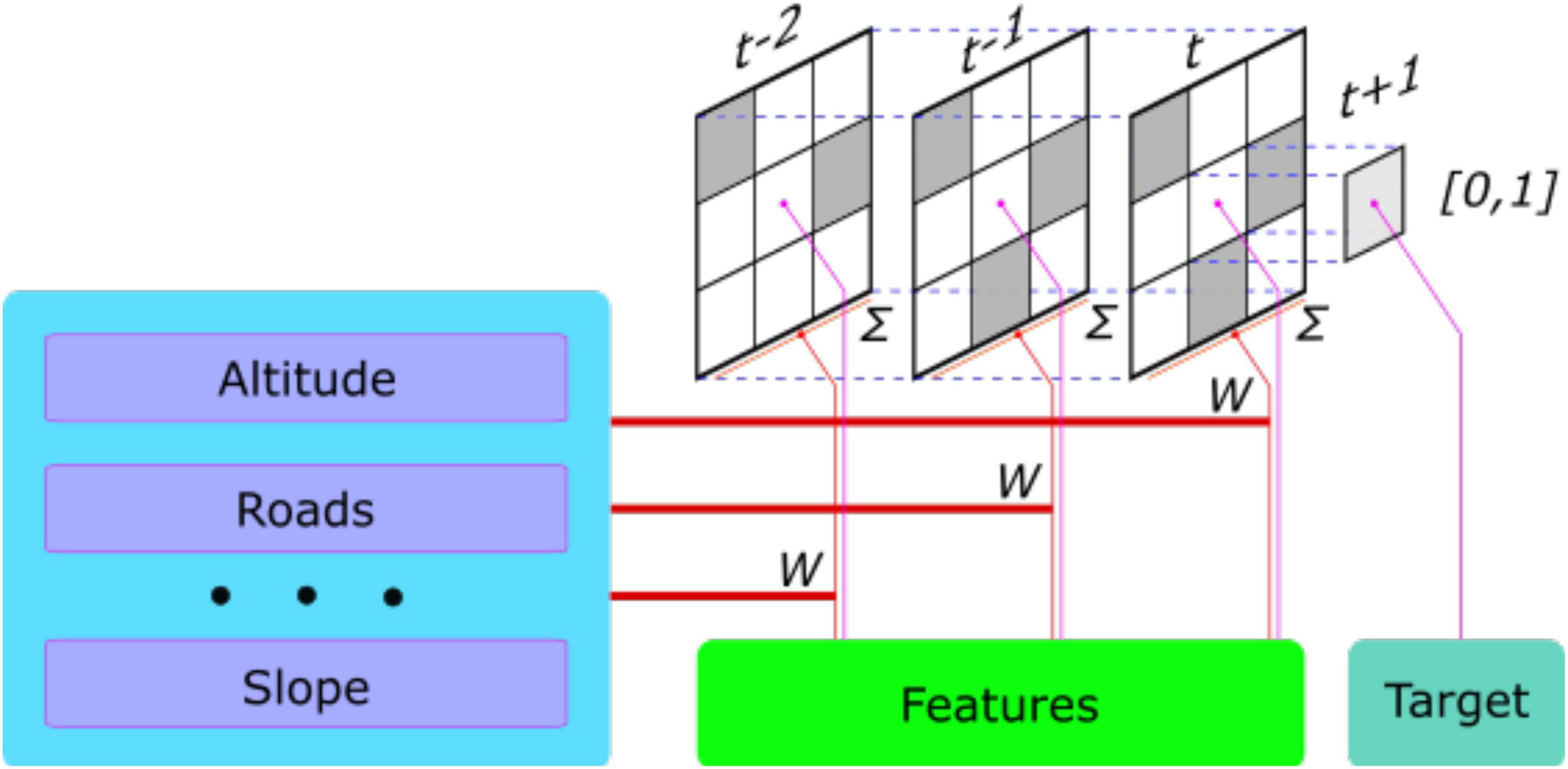
Figure 3. Scheme of feature collection.

The regression model takes the following form:

$d_{ij}\left(t+1\right)=\mathrm{}MODEL[W_{ij}^k,{\displaystyle \sum H_{ij}\left(t\right)},{\displaystyle \sum H_{ij}\left(t-1\right)},\mathrm{\hspace{1em}}\hspace{1em}{\displaystyle \sum W_{ij}^l\left(t\right)},{\displaystyle \sum W_{ij}^l\left(t-1\right)}],$

$k=1,..,K,l=1,..,L,L=K(2)$

Where d_ij(t) is decayed deforestation in the cell (i,j) at time t,d_ij ∈ [0,1]. Here, $W_{ij}^k,k=1,..,K,$ are stationary features in cell (i,j); they are components of K matrices $W^k=\left(W_{ij}^k\right)\in {ℝ}^{Q\times P}$. Variables corresponding to stationary features are provided in Table 2, where K = 11.

TABLE 2

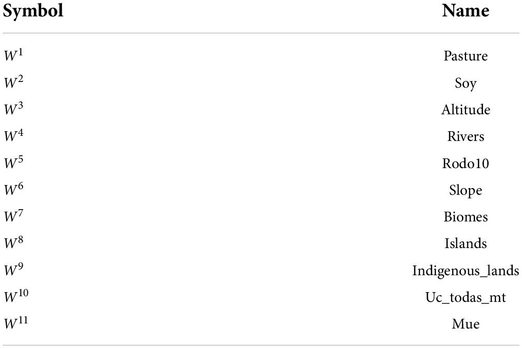
Table 2. Stationary features in the regression model (see Eq. 2).

∑H_ij(t) is the sum of targets in the neighborhood of cell (i,j) at time t and has the form:

$\sum H_{ij}\left(t\right)=\sum _{r=-1}^1\sum _{s=-1}^1{d}_{i+rj+s}(t)(3)$

$\sum W_{ij}^l\left(t\right),l=1,..,L,$ is a convolution of selected features $W_{ij}^l$at cell (i,j) at time t, described by the formula:

$\sum W_{ij}^l\left(t\right)=\sum _{r=-1}^1\sum _{s=-1}^1\left(d_{irjs}\left(t\right)-0.5\right)\cdot W_{i+rj+s}^l(4)$

Convolution $\sum W_{ij}^l\left(t\right),l=1,..,L,$ determines the direction of deforestation spread and shows interaction between adjacent cells in the neighborhood of grid cell (i,j). W^l_ij are L selected features from K = L stationary features $W_{ij}^k.$We considered only numerical features. The sum of neighboring cells in Eq. 3 is symmetrical by default. However, in Eq. 4 we couple it with other features. This helps us make the influence asymmetrical because it is adjusted to additional factors, which in general vary around each cell. Those features complement the actual impact of deforestation as defined in Eq. 3.

We must note that since d_ij(t) can often be zero, we lose information about features in such neighboring cells during the convolution operation (Eq. 4). To eliminate this, we rescaled it by subtracting 0.5 from d_ij(t) (see Eq. 4). As the result, we construct L matrices $\sum W^l\left(t\right)=\left(\sum W_{ij}^l(t)\right)\in {ℝ}^{Q\times P}$ containing additional time-dependent features.

Table 3 provides variable names for new features ∑W^l(t), ∑H(t), where L = 6.

TABLE 3

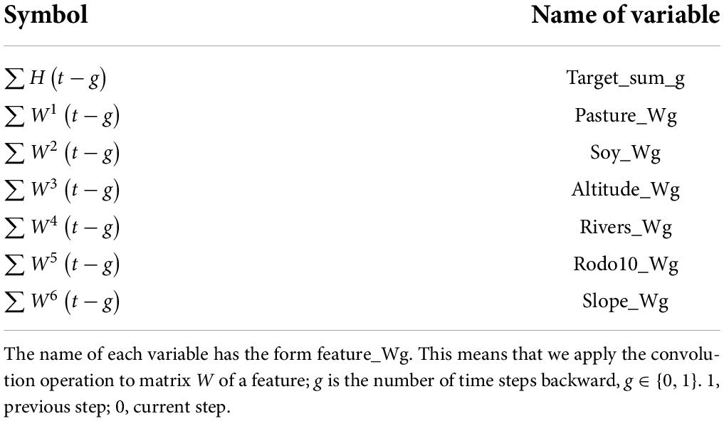
Table 3. Time-dependent features and their names.

In our model, we account for both the current and previous time steps. We consider an iterative process of feature formation. After each iteration d_ij(t + 1) = MODEL[⋅], we obtain matrix D(t + 1) = (d_ij(t + 1)) ∈ ℝ^{Q × P} of decayed deforestation, which is used for the feature formation:

${\displaystyle \sum W^l\left(t+1\right)}=\left({\displaystyle \sum W_{ij}^l(t+1)}\right)\in {ℝ}^{Q\times P},$

${\displaystyle \sum H\left(t+1\right)}=\left({\displaystyle \sum H_{ij}(t+1)}\right)\in {ℝ}^{Q\times P}.$

Mato Grosso boundaries are used as spatial constraints, assuming that deforestation beyond the state boundaries is equal to zero. Hence, d(t) = 0 is fixed for grid cells on the border and outside of Mato Grosso for all t.

For model training, we created a dataset with target variable D(t), t ∈ [t₀,T] and the corresponding variables from Tables 2, 3. First, we created a dataset for the entire area and all time steps. This dataset contains all features used in the model (see Eq. 2). Second, we split this dataset randomly into the train and test sets in the proportion of 70 to 30%. We solved the regression problem in Eq. 2 using the LGBMRegressor method from the LightGBM gradient boosting framework (Ke et al., 2017). For tuning model parameters, we used the train set. We applied K-fold cross validation with five folds and a randomized search of parameters through the grid of fixed range. To assess model quality, we considered the coefficient of determination R². This represents the proportion of variance of decay deforestation that is explained by independent variables in the model. After validation on the test set, we obtained an R² score of 0.455. The features, sorted by their importance in the model, are given in Table 4. The most important features are those dealing with neighboring cells. Therefore, this outcome confirms our hypothesis about deforestation drivers.

TABLE 4

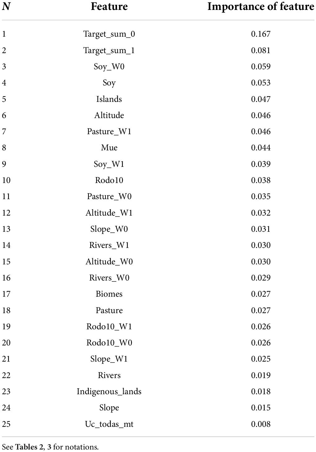
Table 4. The importance of features used in the model.

A predictable initial reaction to some of the relatively small R² scores is that perhaps the correlation is not as expansive as we might have predicted. However, taking into account the presence of random deforestation in the historical data that is explained neither by internal factors nor interaction with neighboring cells provides helpful context. The appearance of a correlation, however, slight, indicates that there is a relationship between the two variables that is statistically significant despite the preponderance of seemingly random deforestation. In the simulation portion of this paper, we propose a Monte Carlo approach to allow such random deforestation events to be taken into account.

During model training we did not force barriers (e.g., Indigenous lands and conservation units) to be unavailable for deforestation. However, based on the historical data the model learned to consider those areas as having a very low probability for deforestation.

Simulation of scenarios

The trained model allows the assessment of the spatial dynamics of deforestation probabilities. After decaying past deforestation, we predict “probabilities of deforestation” as target variables, represented by values from 0 to 1, in the cells where no deforestation has previously occurred.

In order to identify an event of deforestation, we set a threshold value N. As soon as this threshold is reached, the pixel is marked as 1 and is considered to be deforested, and the decay factor is applied in all next time steps. Once a pixel is deforested, we don’t apply any other operations except decaying. Thresholds are applied to deforestation probabilities only in pixels marked as 0, i.e., standing forest land. Therefore, we track two maps in parallel:

• A map of probabilities, including both deforested and forested pixels.

• A map of 0’s and 1’s (e.g., the status of each pixel).

We use the first map for modeling and the second for model output.

In modeling thresholds, we apply both deterministic and probabilistic approaches. In a deterministic case, we deal with the prescribed deforestation thresholds. In a probabilistic approach, we use Monte Carlo to identify deforestation events at each step. For this purpose, we add random deforestation by the following rule:$\tilde{u}=a\cdot u^b$, where u ∈ Uniform(0,1), where a, b are parameters. We set a = 1 and b = 0.5³.

Considering both probabilistic and deterministic thresholds, the current threshold is defined by the formula:$N_f=\text{min}\{\mathrm{N},\tilde{u}\}$, where N is the deterministic threshold. Therefore, deforestation takes place either when a fixed threshold N is reached or if there is a random event that indicates it could happen at the lower threshold $\tilde{u}$.

For this purpose, we chose a random threshold from a transformation of a uniform distribution, as illustrated in Figure 4. This helps to reduce the chances of obtaining very low values for probabilistic thresholds that would result in an immediate deforestation of many grid cells. For example, if the random number generator draws the value u = 0.2 it is transformed to $\tilde{u}$ = 0.447.

FIGURE 4

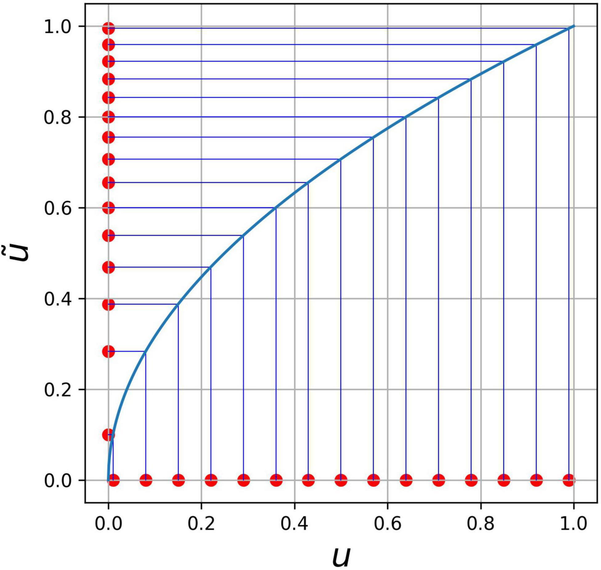
Figure 4. Transformation of random threshold u from uniform distribution into threshold $\widetilde{\mathbf{\text{u}}}$.

The simulation runs through 2050. We use the interval 2010–2019 for model initialization, and then, from 2020 onward, we introduce the thresholds. During the initialization period, only probabilistic thresholds are implemented. Initialization is necessary for the model to reach a stable mode of operation. During this interval, the nearest-neighbor mechanism manifests itself sharply and some time is needed for saturation of this mechanism to normal mode. This happens because we do not have any fixed time interval during the training period, as we take arbitrary subsets of data for learning and testing, which differs from the time-series approach.

Figure 5 illustrates historical deforestation dynamics (2000–2016) shown by blue trajectory and simulation results during (2010–2019) shown in red color both in terms of annual and cumulative values. Number of deforested cells was 284 thousands in 2000 and had a rapid growth until 2005 when it reached 342 thousands. The area of a cell is 1 km². Then the rates were reduced to around 2 thousands cells per year by 2010 resulting in 364 thousands cells. The growth rate stabilized until 2016 leading to cumulative value of 373 thousands cells in 2016. Simulation started in 2010 and resulted in a sharp increase of annual rates from 1.5 thousands cells per year in 2010 to 3.5 thousands cells per year in 2011. This is explained by activation of the neighboring mechanism proposed in the study, which to some extent replicated historical behavior from 2000. By 2019 the growth rate stabilized and reached the level of 1.47 thousands cells per year. The cumulative values show that although simulation results (red line) is above the historical data (blue line) during 2010–2016, simulation results satisfactory replicate historical deforestation trend. We assumed that the model setup the results presented in the figure was good enough for our research objectives, which deal more with the future policy impacts on deforestation dynamics, rather than with replicating the historical period.

FIGURE 5

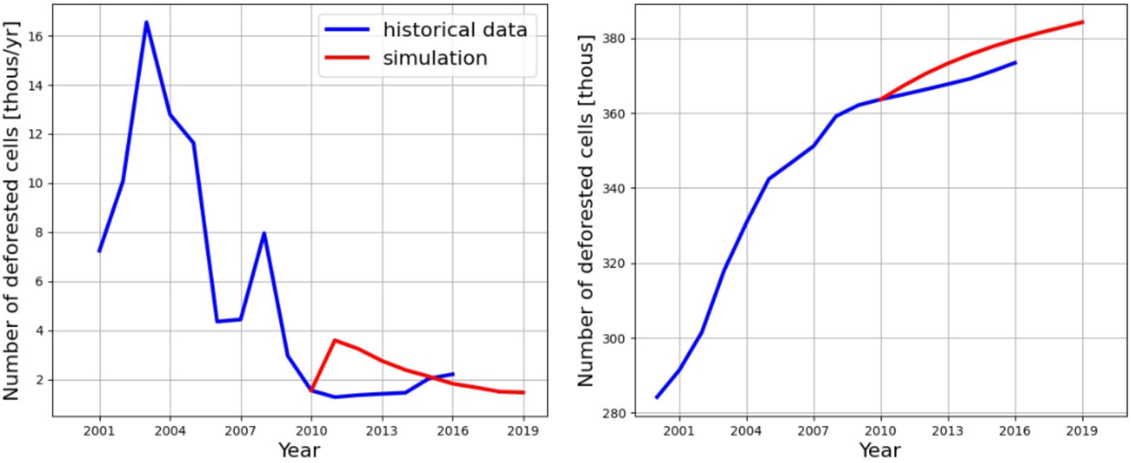
Figure 5. Historical deforestation dynamics (2000–2016) and simulation results during the model initialization (2010–2019) both in terms of annual (left) and cumulative (right) values.

Figure 6 shows how the threshold part of our model works. For illustration, we set a deterministic threshold to N = 1, meaning that deforestation should never happen. Therefore, the only active threshold is probabilistic — i.e., a random draw can set a value below 1 in some cells, thus potentially leading to deforestation due to accidental exogenous factors, such as fire. One can see that deforestation rates are declining in this case, but are still positive. Five simulations are shown in this figure in addition to the average values. It can be seen that randomization is reasonable and does not produce any explosive effects — i.e., the spread of stochastic runs around the mean is bounded. In all simulations deforestation falls from about 1,500 km² per year to about 700 km² per year by 2050.

FIGURE 6

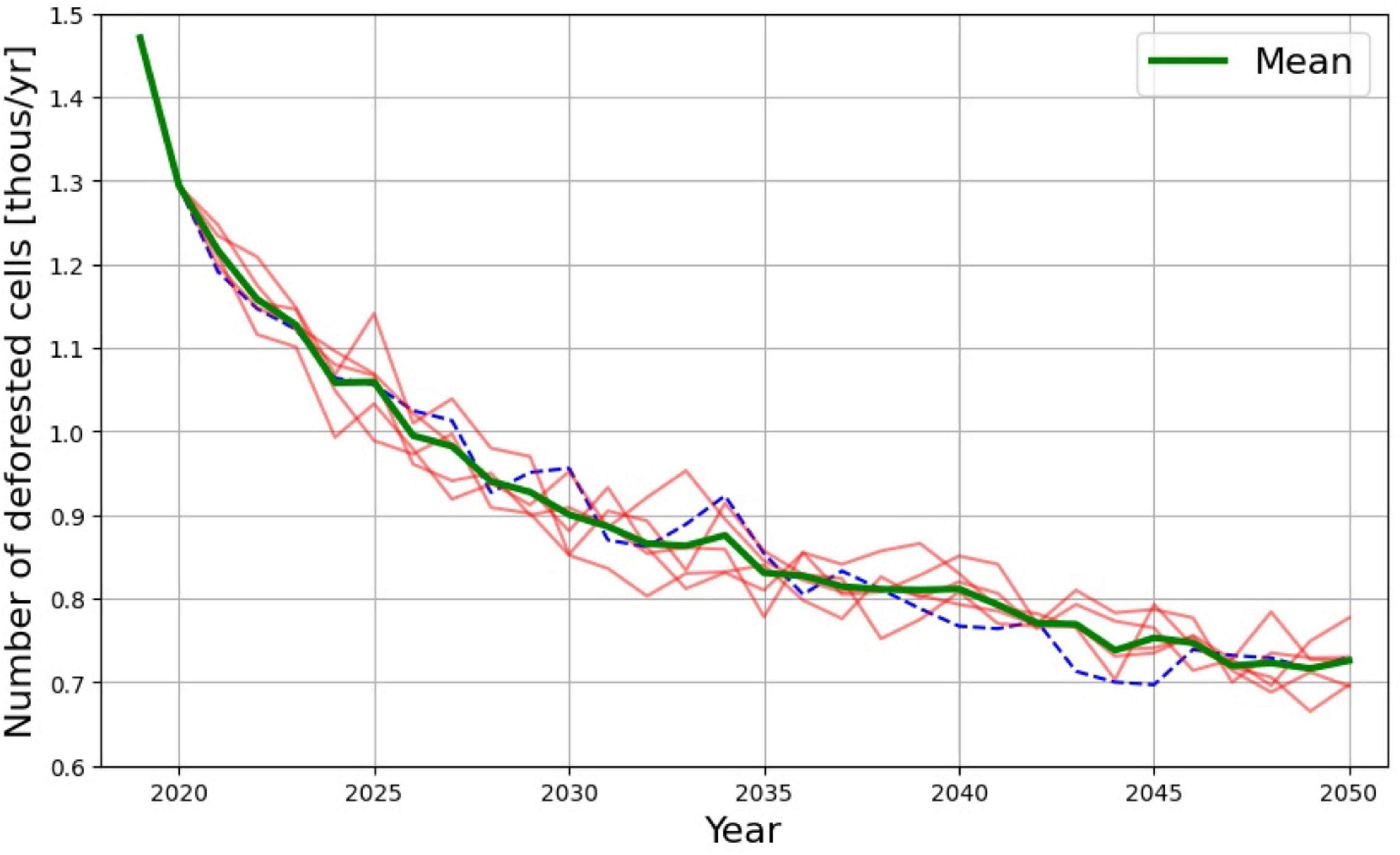
Figure 6. Deforestation scenario with threshold N=1. Deforestation rates are the number of deforested cells per year. The green line represents the mean of stochastic simulations. The dashed blue line represents a stochastic simulation used in the “Results” section. Other lines are representative of individual model runs. The spread of stochastic runs around the mean is bounded.

A more realistic situation is when the threshold is set to N = 0.35 for the entire area. The dynamics of deforestation rates in this case are shown in Figure 7. We consider this scenario as the baseline for our future runs. The deforestation rate increase to 1.84 thousands cells per year in 2020 that is compatible with 2.2 thousands cells per year in historical period 2016 as shown in Figure 5. One can see that in terms of deforestation rates the model shows an inverted U-shaped behavior. At first, the number of deforested cells grows at an increasing rate until the growth rate reaches its maximum. After its peak, growth starts to saturate. This behavior would result in the S-shaped curves in cumulative values shown in Figure 8. We also present several Monte Carlo runs, showing that deviation from the mean is less than 10%. The concave shape in Figure 7 is explained by the decreasing number of cells available for deforestation, because we do not model any afforestation in this study. This pattern of deforestation dynamics is found in other studies (e.g., Lubowski et al., 2014). The falling rate of deforestation during the period 2035–2050 illustrates a rather catastrophic situation: at this stage the number of deforested cells is so high that the spread slows down because of this.

FIGURE 7

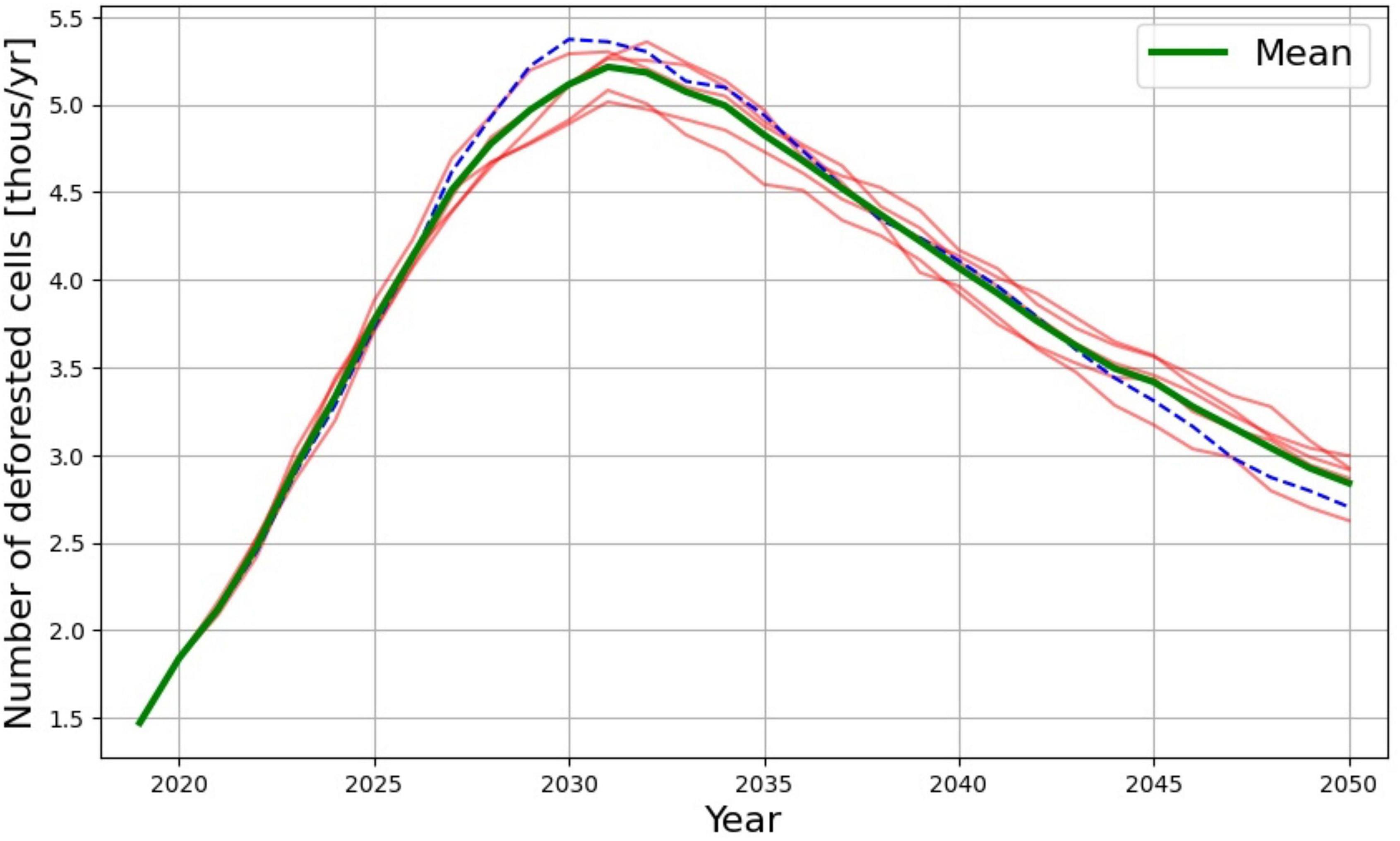
Figure 7. Deforestation scenario with threshold N=0.35. Deforestation rates are the number of deforested cells per year. The green line represents the mean of stochastic simulations. The dashed blue line represents a stochastic simulation used in the “Results” section. Other lines are representative of individual model runs. The spread of stochastic runs around the mean is bounded.

FIGURE 8

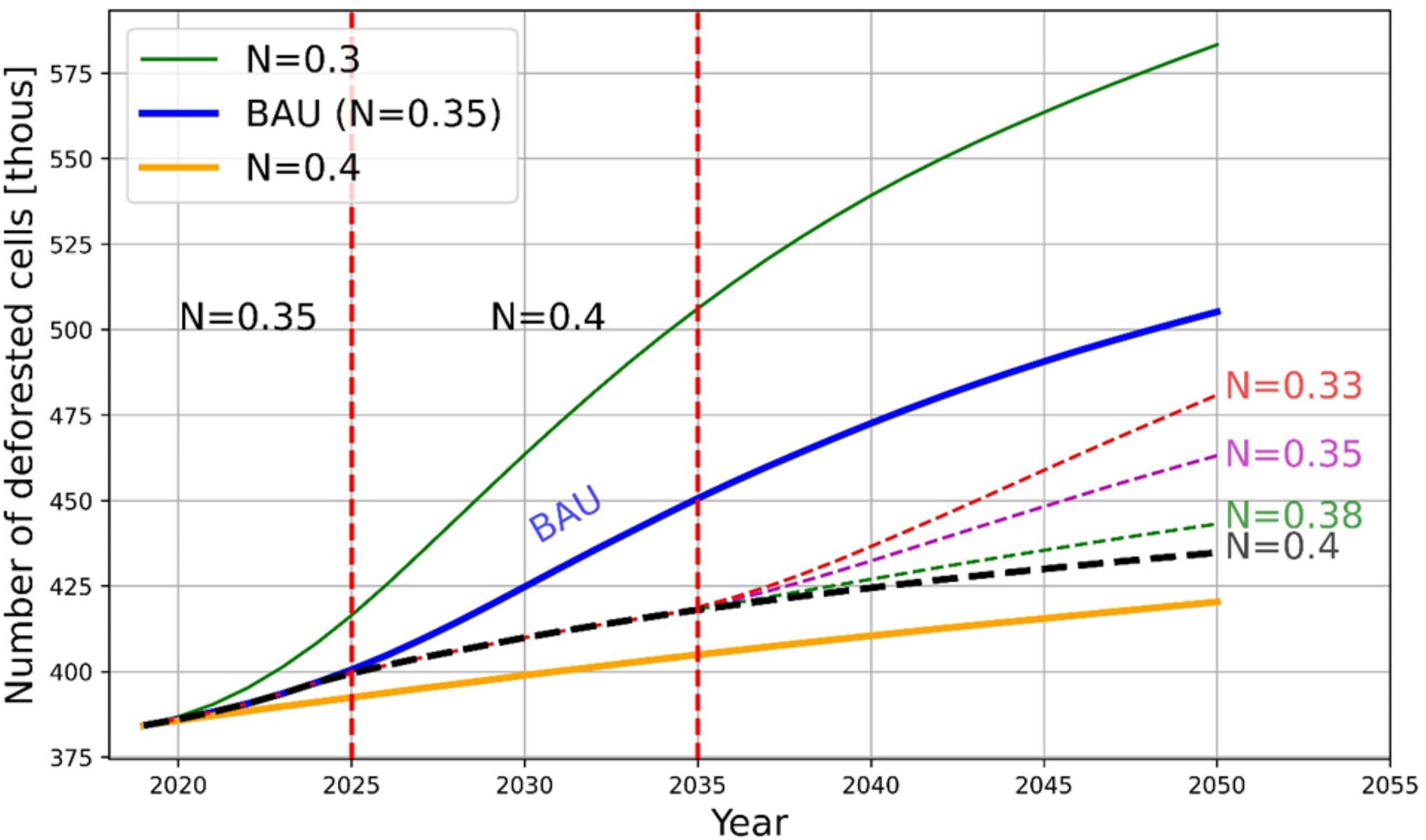
Figure 8. Cumulative number of deforested cells.

Results

In this section we present results of our simulated policy intervention at the jurisdictional scale.

First, we modeled a jurisdictional command-and-control policy affecting the state of Mato Grosso. We simulate a tightening of law enforcement to curb deforestation during the period 2025–2034 by increasing the threshold at which cells are deforested compared to BAU, implemented by shifting from N = 0.35 to N = 0.4.

Next, in order to understand the permanence of avoided deforestation and related carbon emissions from this command-and-control policy intervention, we modeled four different scenarios. First, the tighter law enforcement policy (N = 0.4) is maintained throughout 2050.

Then, we modeled three alternative levels of law enforcement loosening by decreasing the threshold of deforestation for all cells across the jurisdiction to N = 0.38, N = 0.35 (BAU value) and N = 0.33. This captures the possibility of a policy rollback triggered in 2035.

Our simulations allow us to understand the intertemporal effects of such a command-and-control policy and analyze changes in deforestation and emissions patterns in the absence or presence of future policy reversals.

Jurisdictional scenarios with variable thresholds

In this subsection we consider scenarios applied to all the cells, i.e., jurisdictional policies.

Figure 9 shows the dynamics of deforested cells in each year during the period 2020–2050. The orange, blue, and green lines show the dynamics for thresholds 0.4, 0.35, and 0.3, correspondingly.

FIGURE 9

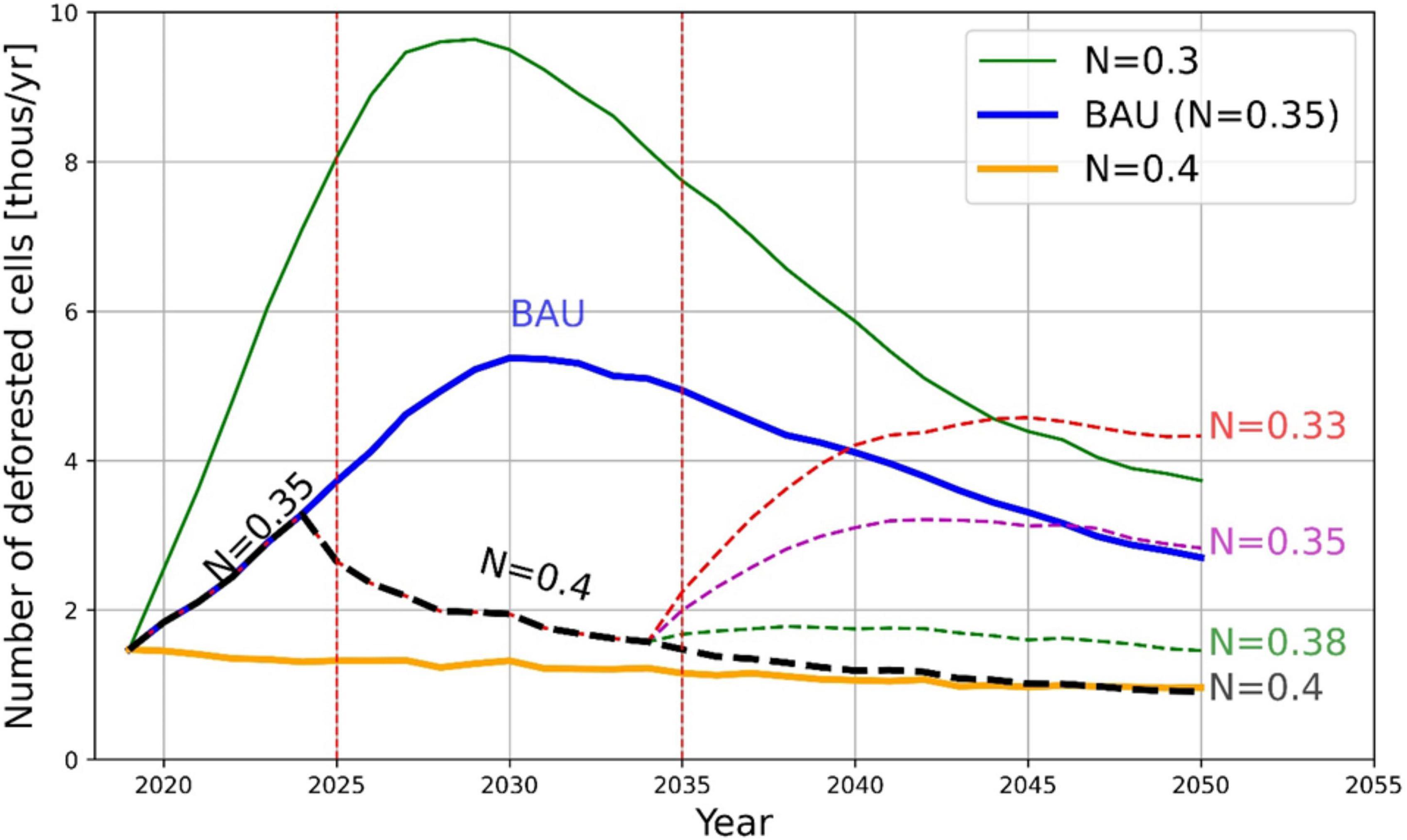
Figure 9. Deforestation scenarios under jurisdictional policies.

Our simulations show that the range for thresholds is between 0.3 and 0.4 — i.e., the model is quite sensitive to the changes in thresholds⁴. This is connected with other parameters of the model as well as the chosen decay rates and time scale. We set the 0.35 threshold as the baseline; 0.4 corresponds to a tighter law enforcement and lower deforestation pressure, and threshold 0.3 is a rather extreme scenario of loose law enforcement and deforestation boom.

In the first scenario we introduce a policy intervention from 2025 to 2034 to slow down the BAU deforestation by increasing the threshold from 0.35 to 0.4. One can see the positive effect of this policy in Figure 9: the blue trajectory is switched to the black dashed line. If this policy were to be kept, deforestation would decline until 2050. However, if from 2035 to 2050 we change the threshold value of 0.4 to lower values, we see that deforestation rises again. Although the period of tight deforestation control has its positive effects, deforestation rates reach the BAU levels in 2050 (magenta dashed line; N = 0.35) or can go even higher (red dashed line; N = 0.33) if the new threshold is lower than the BAU threshold. At a threshold of N = 0.38, the green dashed line, deforestation stays below the BAU trajectory. The purpose of experimentation with different thresholds is to detect a critical level after which avoided deforestation could be treated as permanent.

Figure 8 illustrates the cumulative deforestation values corresponding to the annual deforestation in Figure 9. Here, we observe that temporary deforestation control (2025–2034) has positive permanent effects even if the policy is rolled-back: in cumulative values all the dashed curves are below the BAU curve by 2050.

Nevertheless, because of the high deforestation rates at threshold N = 0.33 following the end of deforestation control in 2034 shown in Figure 9, there is a possible negative outlook after 2050 in that scenario. The model exhibits permanent effects for N = 0.4 and higher.

Spatial dynamics and barriers against deforestation

The illustration of spatial dynamics of deforestation corresponding to the BAU scenario (Figure 9) is shown in Figure 10 for the years 2035 and 2050. We see that in 2035 the deforestation process is still in an active stage. The hotspots are shown in magenta and red colors. In the future deforestation is happening mainly in the Amazon biome which can be explained by the historical deforestation pattern depicted in Figure 2. In this figure most of the clusters of pixels with high decayed values in 2010, which drive the future dynamics in the model, are located in the Amazon biome. There are some recent deforestation events in Pantanal, but they are rather isolated, i.e., not forming clusters, and therefore do not activate the proposed neighboring mechanism intensively, leading to low deforestation in the future scenarios. As mentioned in the paper we do not model afforestation and therefore deforestation can happen only in the cells that were not deforested before. This explains relatively low future deforestation patterns in Cerrado due to the fact that it was intensely deforested in the historical period (see Figure 2). The deforestation process is well illustrated in particular by comparing the areas in 2035 and 2050 on the top-left of the maps. We also show by hatched shading the Indigenous lands where the probability of deforestation is very low. However, we see that deforestation is active at the boundaries of those lands and, in particular, that it will be concentrated in 2050, because it is basically the only patches of forest left by that time. We also see that there are some deforested pixels inside those areas, mostly due to the random events simulated in the model. However, they are not spreading due to their location. Although we do not force probabilities to be zero, the model learned to keep them very low in those lands, thus making Indigenous lands barriers against deforestation.

FIGURE 10

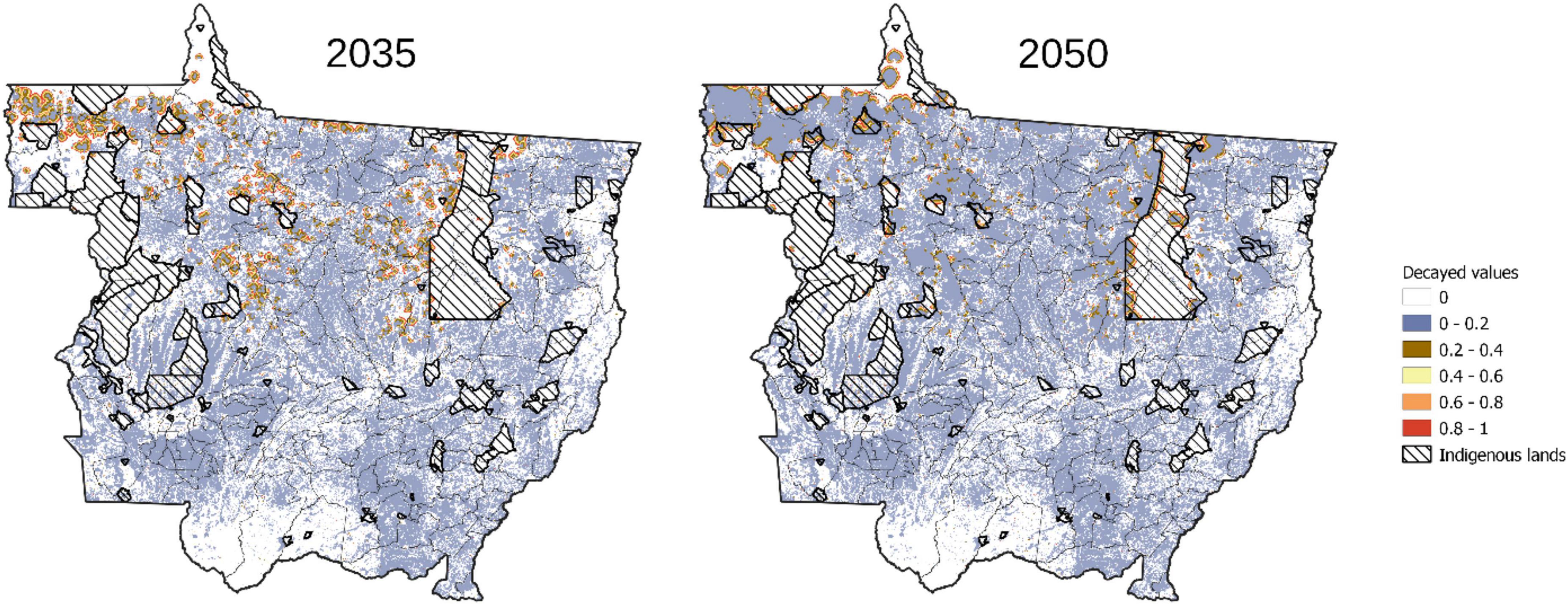
Figure 10. Spatial dynamics of deforestation under the BAU scenario for 2035 and 2050, with Indigenous lands acting as barriers against deforestation.

Jurisdictional policy impacts

Here we consider how jurisdictional policies would impact deforestation dynamics in the region according to our model, following the native vegetation preservation requirements from the 2012 Brazilian Forest Code. We use the following maps as a basis for modeling scenarios: a map containing pixels of 1 km² size with native vegetation surplus, and a map representing pixels with native vegetation deficit. Both maps are shown in Figure 11. These maps are based on data from Stabile et al. (2022). The total area of surplus is 7.21 million ha while the total area of deficit is 8.76 million ha.

FIGURE 11

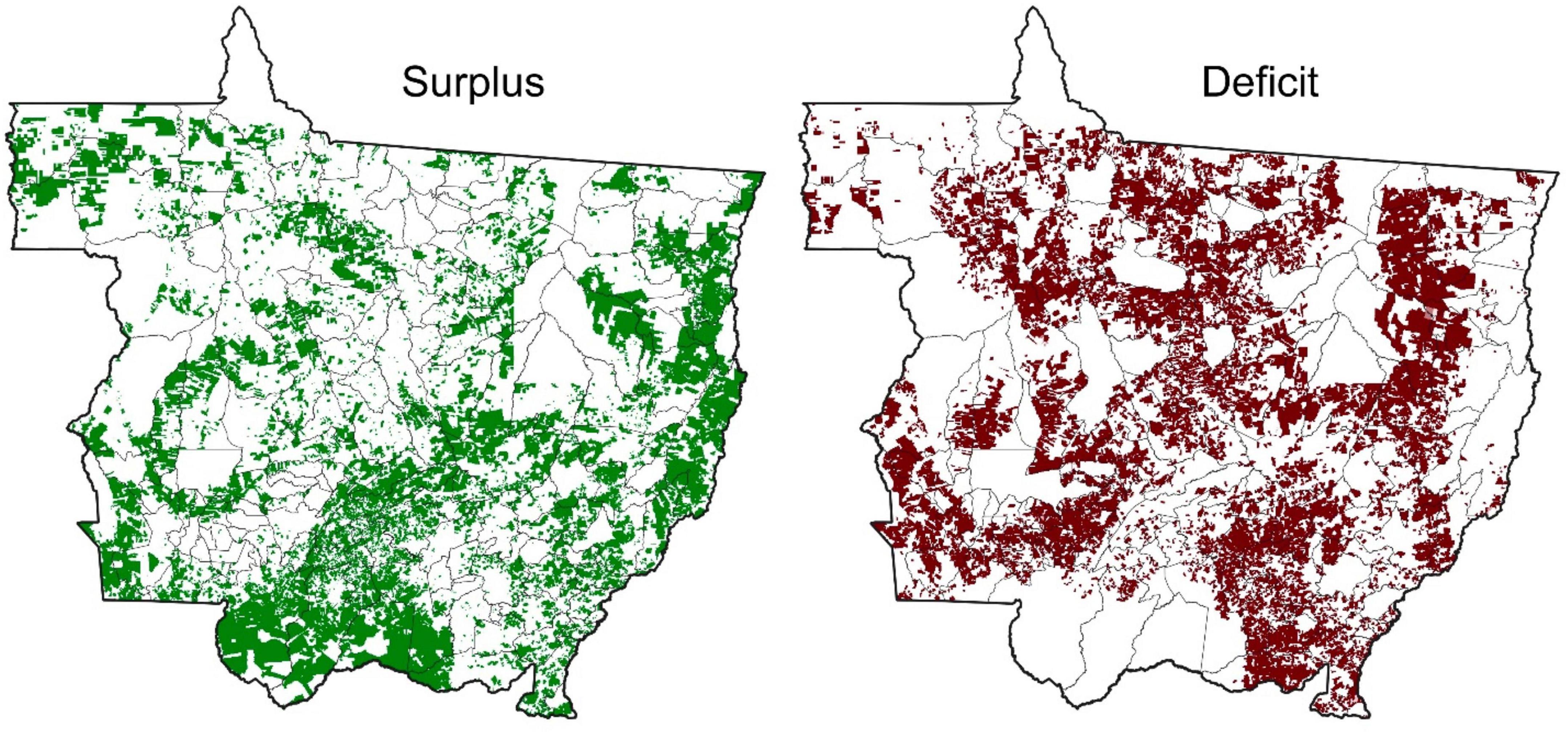
Figure 11. Maps of native vegetation surplus (left) and deficit (right).

We use such maps to simulate two policies concurrently. The first policy simulates an incentive-based jurisdictional program where payments would be made to landowners with native vegetation surplus, thus blocking those parcels from deforestation. The second policy simulates a command-and-control approach to bring properties back to compliance with the Brazilian Forest Code by reforesting their deficits.

First, deforestation was blocked in all areas with a forest deficit from 2010 until 2050. We considered all those pixels as reforested and protected during the entire time interval. At the same time we considered the following cases for areas with forest surplus:

• Case 1 — block deforestation from 2010 until 2050.

• Case 2 — block deforestation from 2010 until 2030 and allow deforestation afterward.

• Case 3 — block deforestation from 2010 until 2030, allow deforestation in the period 2030–2034, and block deforestation afterward.

• Case 4 — block deforestation from 2010 until 2030, allow deforestation in the period 2030–2039, and block deforestation afterward.

Modeling results are presented in Figure 12, where annual numbers of newly deforested pixels are shown for various scenarios. The difference between BAU and jurisdictional policy cases in 2020 is explained by the fact that areas with deficit and surplus were removed at the start of the simulations in 2010. The difference between policy scenarios begins in 2030. The best outcome is achieved in Case 1, where all selected areas are protected by policy until 2050. In that case the rate of deforestation in the study area is consistently low. In Case 2, when policy is relaxed in surplus areas until 2050 we see a relatively fast increase in deforestation rates with a qualitative behavior similar to the BAU scenario; the maximum deforestation rate happens around 2042. Quite interesting effects are observed when the relaxation of policy in 2030 is reversed in 2035 (Case 3) and 2040 (Case 4). The return of the policy to protect areas with forest surplus allows to slow down deforestation rates and gradually converge them to the level of Case 1 by 2050. This shows that due to the high number of pixels where policies are applied, the neighboring effect is one of the key factors for spreading deforestation.

FIGURE 12

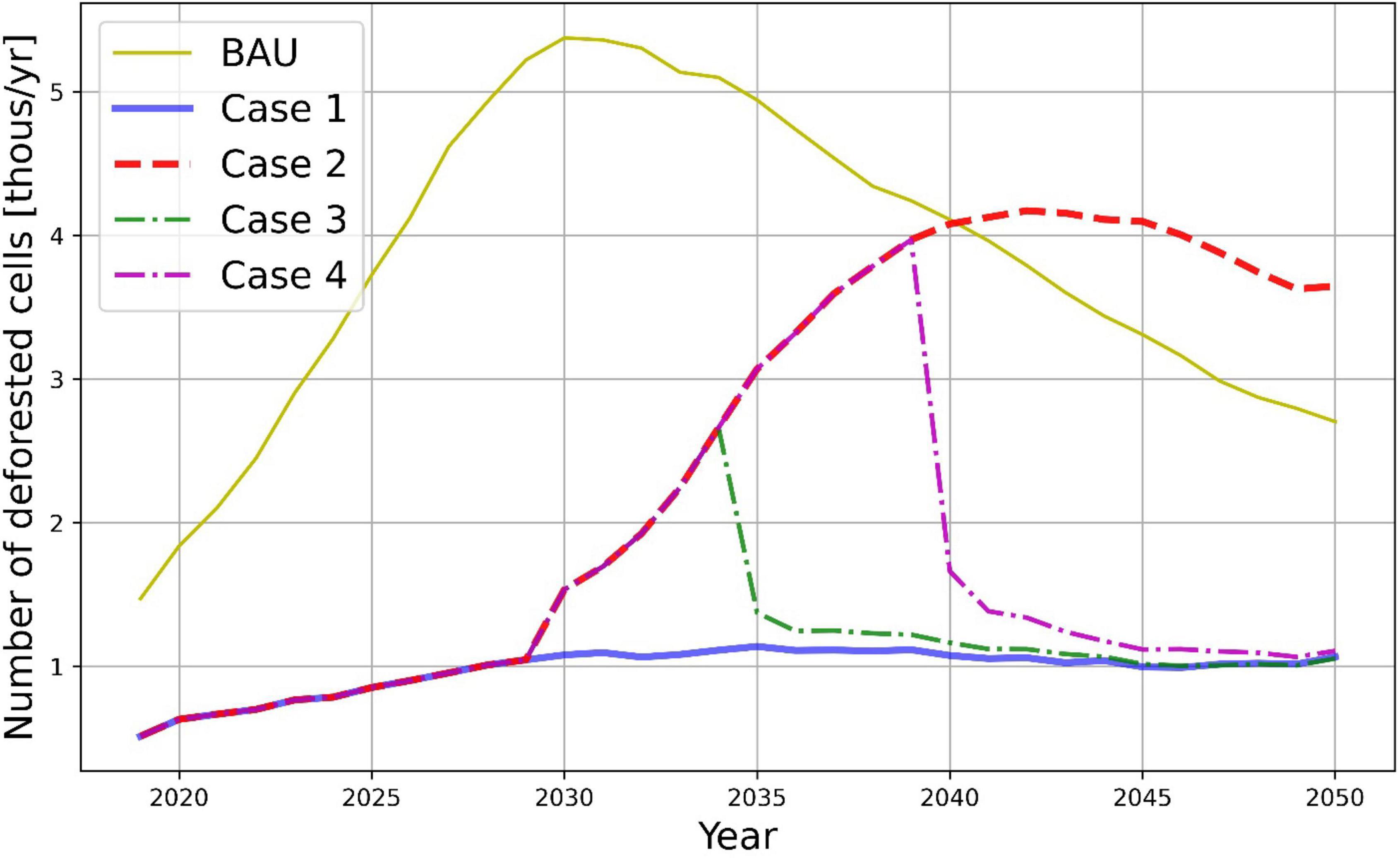
Figure 12. Jurisdictional policy impacts compared to BAU scenario (as in Figure 9). Cumulative deforested areas corresponding to policy scenarios are given in Figure 13. The figure clearly illustrates the impact of policy reversals — i.e., Cases 3 and 4 allow deforestation to be reduced to the levels close to Case 1. This has some analogy with epidemic models, where policies could be considered as quarantine measures that can be forced and relaxed by governments at various time periods.

FIGURE 13

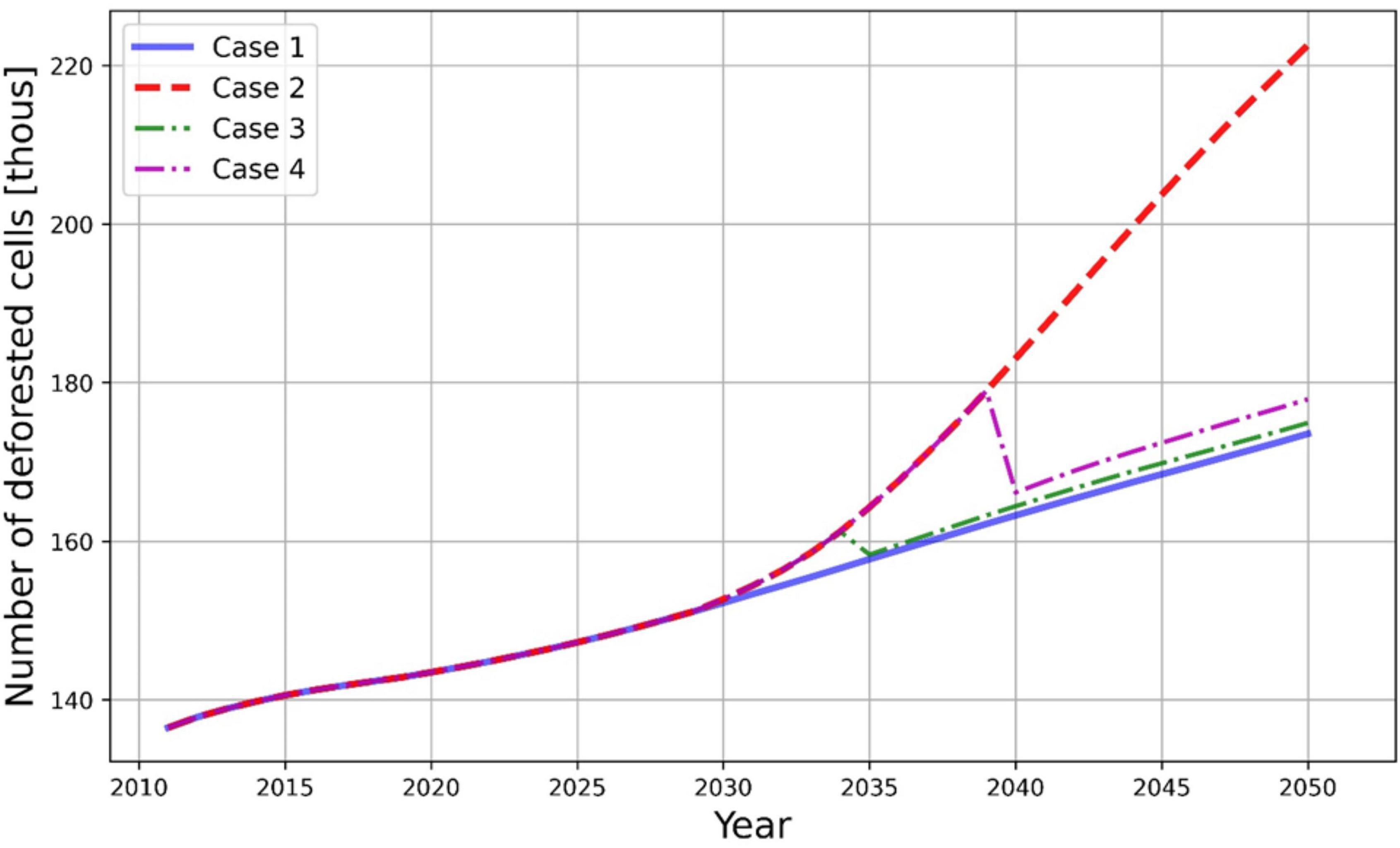
Figure 13. Cumulative number of deforested cells in jurisdictional policy scenarios.

Finally, in Figure 14 we present maps that compare results of deforestation in the BAU scenario and in Case 1 scenario of jurisdictional policy for 2050. We see that due to the dynamics of neighboring pixels that are at the core of the model, the difference in deforested cells is considerable. This is a positive result for policy interventions.

FIGURE 14

Figure 14. Comparison of the BAU scenario (left) and Case 1 scenario for 2050 (right).

Discussion and conclusion

In this paper we analyze the permanence of REDD+ by employing a CA algorithm of endogenous deforestation. We simulate different jurisdictional policy interventions to slow deforestation and promote reforestation and investigate the resulting deforestation patterns under alternative policy scenarios through 2050. Our results suggest strong spatial spillovers from past deforestation, path dependence and partial irreversibility of changes in a deforestation pathway. In other words, once deforestation declines from the BAU trajectory, it is unlikely to rebound to BAU. This observation leads to an important policy conclusion — the stronger and the longer the policy interventions to curb deforestation, the less likely it will bounce back.

The permanence of a policy depends on its success to reduce cumulative deforestation and emissions compared to the BAU trajectory. In turn, this depends on the probability that policy rollbacks and the resulting trajectories of deforestation and emissions do not overshoot the BAU trajectory and outpace previously accumulated deforestation or emissions reductions in the long run. Hence, permanence depends both on the probability of policy reversals and the potential of emissions overshooting, and the relevant time horizon to be considered (e.g., 2050, 2100, etc.). Creating a buffer pool of emissions reductions, as requested by jurisdictional REDD+ standards, is a practical solution to extend the effect of a policy intervention limited in time and mitigate potential policy reversals.

The findings of this study also creates a strong case for a jurisdictional approach. Over time, the economy — previously dependent on deforestation — converges to a new low or deforestation-free steady state. The stronger and more prolonged the period of active policy intervention, the better the chances a tropical nation (jurisdiction) will rebalance natural and manmade capital to support low deforestation development pathways. This conclusion has immediate policy relevance — an external intervention, on a jurisdictional scale, should be planned strategically to maximize the catalytic effect for convergence to a lower deforestation steady-state trajectory.

The logical next step for this analysis is the application of optimization in the organization of areas to protect to study the dynamics of clusters of avoided deforestation. Further, experiments with embedded optimization may answer the questions: If we can spatialize interventions, do they affect deforestation in an outsized way? If we reduce deforestation in certain parcels of land, do they affect the deforestation trajectory in different ways?

Future research

Future research will address the impacts of economic incentives, namely a payment program for REDD+, on curbing deforestation and the permanence of avoided emissions. In our future work, we will analyze the effects of a payment program for REDD+ by applying different deforestation restrictions to the model — i.e., size and location constraints to protect certain areas, reflected by boxed areas in the model.

Figures 15, 16 illustrate how we propose to set up these modeled boxes to investigate the impacts of different box locations and sizes on deforestation and permanence. For example, a future scenario might consider making it very difficult to deforest cells within a certain box by setting N = 1 for those cells, while deforestation of cells outside the box would follow the BAU threshold (N = 0.35).

FIGURE 15

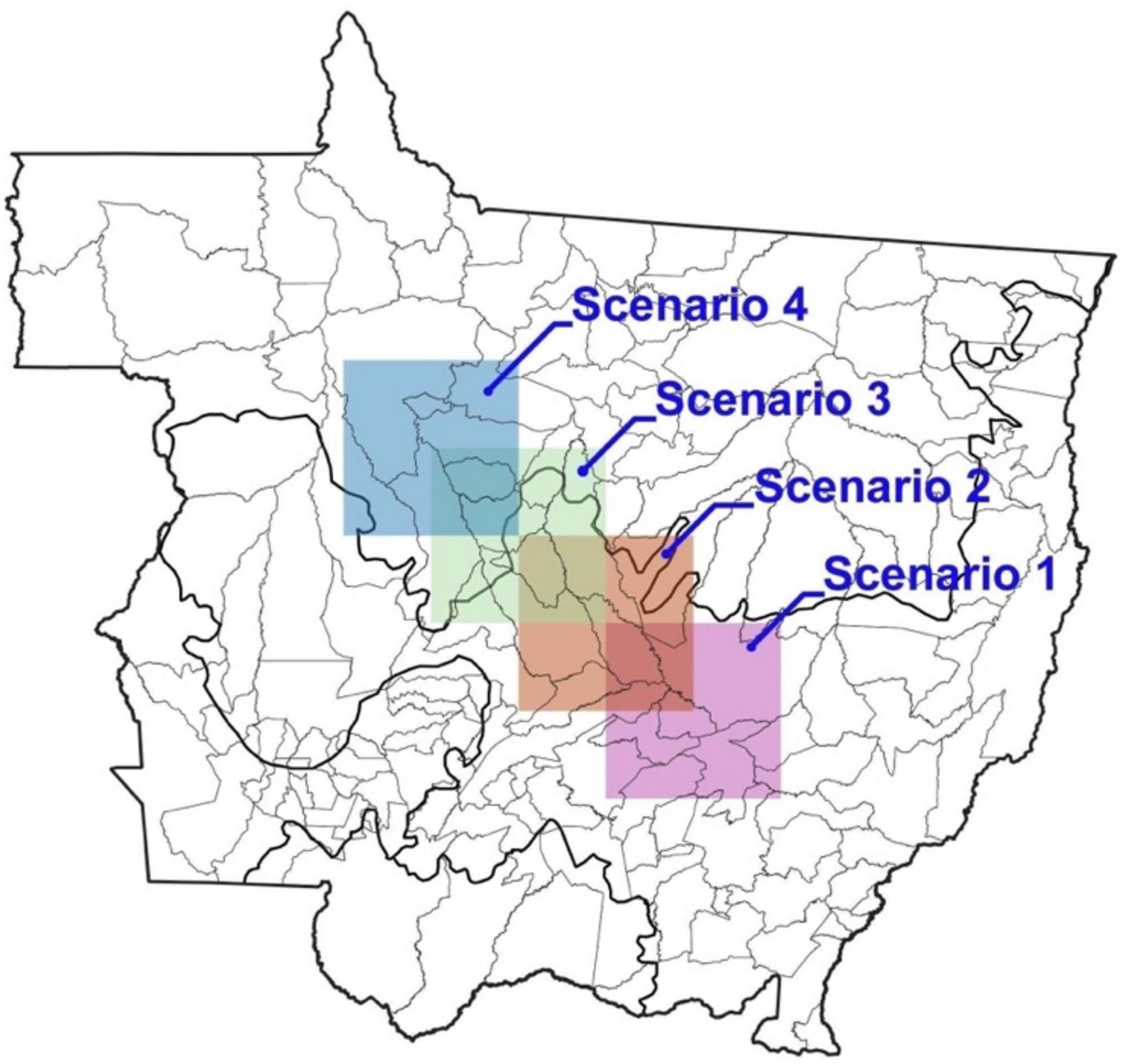
Figure 15. Proposed scenarios with different box locations (shape 200 × 200).

FIGURE 16

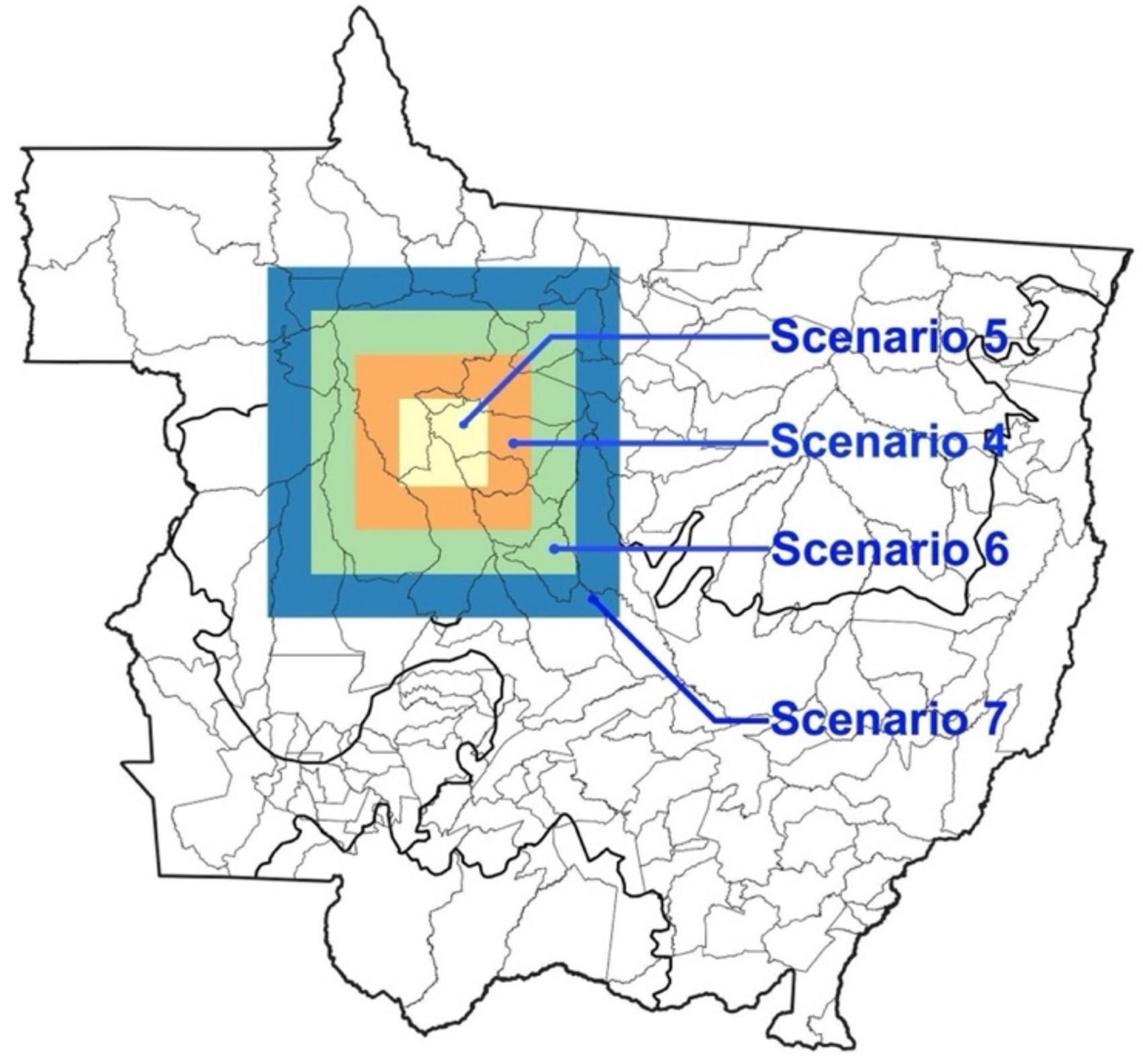
Figure 16. Proposed scenarios with different box sizes: Scenario 5 (100 × 100), Scenario 4 (200 × 200), Scenario 6 (300 × 300), Scenario 7 (400 × 400).

Moreover, we plan to investigate the results of increasing a REDD+ program from project level (small box) to jurisdictional level (the whole state). This will contribute to another heated debate on project versus jurisdictional approaches regarding reducing deforestation.

Another direction for further research is to check for spatial synergies among different small boxes. A REDD+ payment program targeted at rural properties may be scattered across the jurisdiction, where each property could be treated as a separate cell. Yet, using an optimization algorithm we may be able to compare alternative results of conducting localized REDD+ payment interventions versus optimizing deforestation reductions over the landscape, given the same budget. This analysis would help to establish a strategy for scaling up jurisdictional REDD+ programs by maximizing environmental benefits at the minimum cost.

Data availability statement

The datasets presented in this article are not readily available because the bulk of the dataset is publicly available and can be shared upon request. Data on forest surplus and deficits in Mato Grosso are confidential from IPAM – The Amazon Environmental Research Institute. Software: Python 3.7 with the LightGBM package was used for modeling, QGIS 3.4.12-Madeira and R version 4.0.2 were used for data processing and visualization. Requests to access the datasets should be directed to BP, bpietracci@edf.org.

Author contributions

MM conducted the substantive literature review and coordinated meetings among authors. AK was in charge of modeling efforts and generating figures. AP assisted in modeling efforts and figures generation. BP supplied data, consulted with modelers, and provided many rounds of feedback and editing. GL offered suggestions based on GL’s familiarity with the topic of deforestation generally and Mato Grosso specifically. RL offered suggestions based on RL’s expertise in the topic of deforestation. AG consulted with modelers and provided feedback and review. All authors contributed to the article and approved the submitted version.

Funding

This work has been supported by the Norwegian Aid Agency (NORAD) via grant Norad-QZA-0464, QZA-16/1218: “Delivering Incentives to End Deforestation: Global Ambition, Private/Public Finance, and Zero-Deforestation Supply Chains.” This research was also supported by the RESTORE+ project (www.restoreplus.org), which is part of the International Climate Initiative (IKI), supported by the Federal Ministry for the Environment, Nature Conservation and Nuclear Safety (BMU) based on a decision adopted by the German Bundestag.

Conflict of interest

The authors declare that the research was conducted in the absence of any commercial or financial relationships that could be construed as a potential conflict of interest.

Publisher’s note

All claims expressed in this article are solely those of the authors and do not necessarily represent those of their affiliated organizations, or those of the publisher, the editors and the reviewers. Any product that may be evaluated in this article, or claim that may be made by its manufacturer, is not guaranteed or endorsed by the publisher.

Footnotes

1. ^ This data does not include forest degradation.
2. ^ We keep the decay factor constant as a baseline for illustrative purposes. However, calibration of the decay factor is an interesting study itself, because it determines the degree to which past deforestation impacts the future one. Perhaps, this factor could be spatially explicit or clustered by regions, and even scenarios. This is a topic for future work.
3. ^ These values represent the degree of random deforestation and are fixed in this study. However, sensitivity analysis could be done in the future to better capture this effect, although it is a difficult task due to its random nature.
4. ^ We fix this range of thresholds (between 0.3 and 0.4) for illustration in this study. However, threshold values would vary with respect to decay factor. Therefore, simultaneous calibration of the decay factor and threshold values could be done in the future.

References

Acheampong, E. O., Macgregor, C. J., Sloan, S., and Sayer, J. (2019). Deforestation is driven by agricultural expansion in Ghana’s forest reserves. Sci. Afr. 5:e00146. doi: 10.1016/j.sciaf.2019.e00146

CrossRef Full Text | Google Scholar

Assunção, J., and Rocha, R. (2016). Rural Settlements and Deforestation in the Amazon (Climate Policy Initiative Working Paper). San Francisco, CA: Climate Policy Initiative.

Google Scholar

Barbier, E. B. (2004). Explaining agricultural land expansion and deforestation in developing countries. Am. J. Agric. Econ. 86, 1347–1353. doi: 10.1111/j.0002-9092.2004.00688.x

CrossRef Full Text | Google Scholar

Bowles, I. A., Rice, R. E., Mittermeier, R. A., and da Fonseca, G. A. (1998). Logging and tropical forest conservation. Science 280, 1899–1900. doi: 10.1126/science.280.5371.1899

CrossRef Full Text | Google Scholar

Chen, G., Powers, R. P., de Carvalho, L. M., and Mora, B. (2015). Spatiotemporal patterns of tropical deforestation and forest degradation in response to the operation of the Tucuruí hydroelectric dam in the Amazon basin. Appl. Geogr. 63, 1–8. doi: 10.1016/j.apgeog.2015.06.001

CrossRef Full Text | Google Scholar

Fearnside, P. M. (1982). Deforestation in the Brazilian Amazon: how fast is it occurring? Interciencia 7, 82–85.

Google Scholar

Fuss, S., Golub, A., and Lubowski, R. (2021). The economic value of tropical forests in meeting global climate stabilization goals. Glob. Sustain. 4, 1–11. doi: 10.1017/sus.2020.34

CrossRef Full Text | Google Scholar

Geist, H. J., and Lambin, E. F. (2002). Proximate causes and underlying driving forces of tropical deforestation: tropical forests are disappearing as the result of many pressures, both local and regional, acting in various combinations in different geographical locations. BioScience 52, 143–150.

Google Scholar

Harris, N. L., Gibbs, D. A., Baccini, A., Birdsey, R. A., De Bruin, S., Farina, M., et al. (2021). Global maps of twenty-first century forest carbon fluxes. Nat. Clim. Change 11, 234–240. doi: 10.1038/s41558-020-00976-6

CrossRef Full Text | Google Scholar

International Policy Centre for Inclusive Growth, Institute for Applied Economic Research, and Environmental Defense Fund (2019). International Seminar Business Opportunities for a Sustainable Rural Economy: The Contribution From Forests and Agriculture. Brasília: International Policy Centre for Inclusive Growth.

Google Scholar

Islam, K., and Sato, N. (2012). Deforestation, land conversion and illegal logging in Bangladesh: the case of the Sal (Shorea robusta) forests. iForest Biogeosci. For. 5:171. doi: 10.3832/ifor0578-005

PubMed Abstract | CrossRef Full Text | Google Scholar

Ke, G., Meng, Q., Finley, T., Wang, T., Chen, W., Ma, W., et al. (2017). LightGBM: a highly efficient gradient boosting decision tree. Adv. Neural Inform. Process. Syst. 30, 3146–3154. doi: 10.1016/j.envres.2020.110363

PubMed Abstract | CrossRef Full Text | Google Scholar

Kissinger, G., Herold, M., and De Sy, V. (2012). Drivers of Deforestation and Forest Degradation: A Synthesis Report for REDD+ Policymakers. Available online at: https://www.cifor.org/knowledge/publication/5167 (accessed Feburary 4, 2022).

Google Scholar

Lubowski, R., Wright, M., Ferretti-Gallon, K., Arana, A. J. M., Steininger, M., and Busch, J. (2014). Mexico Deforestation Vulnerability Analysis and Capacity Building. Berlin: Springer.

Google Scholar

Mendelsohn, R. (1994). Property rights and tropical deforestation. Oxf. Econ. Pap. 46, 750–756. doi: 10.1093/oep/46.Supplement_1.750

CrossRef Full Text | Google Scholar

Meyer, A. L., Van Kooten, G. C., and Wang, S. (2003). Institutional, social and economic roots of deforestation: a cross-country comparison. Int. For. Rev. 5, 29–37.

Google Scholar

Müller-Hansen, F., Heitzig, J., Donges, J. F., Cardoso, M. F., Dalla-Nora, E. L., Andrade, P., et al. (2019). Can intensification of cattle ranching reduce deforestation in the Amazon? Insights from an agent-based social-ecological model. Ecol. Econ. 159, 198–211. doi: 10.1016/j.ecolecon.2018.12.025

CrossRef Full Text | Google Scholar

Parsons, J. A., and Fonstad, M. A. (2007). A cellular automata model of surface water flow. Hydrol. Process. Int. J. 21, 2189–2195. doi: 10.1002/hyp.6587

CrossRef Full Text | Google Scholar

Schwartzman, S., Lubowski, R. N., Pacala, S. W., Keohane, N. O., Kerr, S., Oppenheimer, M., et al. (2021). Environmental integrity of emissions reductions depends on scale and systemic changes, not sector of origin. Environ. Res. Lett. 16:091001.

Google Scholar

Sirakoulis, G. C., Karafyllidis, I., and Thanailakis, A. (2000). A cellular automaton model for the effects of population movement and vaccination on epidemic propagation. Ecol. Model. 133, 209–223. doi: 10.1016/S0304-3800(00)00294-5

CrossRef Full Text | Google Scholar

Soares-Filho, B. S., Cerqueira, G. C., and Pennachin, C. L. (2002). DINAMICA — a stochastic cellular automata model designed to simulate the landscape dynamics in an Amazonian colonization frontier. Ecol. Model. 154, 217–235. doi: 10.1016/S0304-3800(02)00059-5

CrossRef Full Text | Google Scholar

Sonter, L. J., Herrera, D., Barrett, D. J., Galford, G. L., Moran, C. J., and Soares-Filho, B. S. (2017). Mining drives extensive deforestation in the Brazilian Amazon. Nat. Commun. 8, 1–7. doi: 10.1038/s41467-017-00557-w

PubMed Abstract | CrossRef Full Text | Google Scholar

Stabile, M. C. C., Garcia, A. S., Salomão, C. S. C., Bush, G., Guimarães, A. L., and Moutinho, P. (2022). Slowing deforestation in the brazilian amazon: avoiding legal deforestation by compensating farmers and ranchers. Front. For. Glob. Change 09:635638. doi: 10.3389/ffgc.2021.635638

CrossRef Full Text | Google Scholar

Trucchia, A., Egorova, V., Butenko, A., Kaur, I., and Pagnini, G. (2019). RandomFront 2.3: a physical parameterisation of fire spotting for operational fire spread models — implementation in WRF-SFIRE and response analysis with LSFire+. Geosci. Model Dev. 12, 69–87. doi: 10.5194/gmd-12-69-2019

CrossRef Full Text | Google Scholar

Tumusiime, D. M., Byakagaba, P., and Tweheyo, M. (2018). Policy and institutional drivers of deforestation. Environ. Policy Law 2, 137–144.

Google Scholar

Verified Carbon Standard (2011). AFOLU Non-Permanence Risk Tool v.3.0.

Google Scholar

West, T. A., Börner, J., and Fearnside, P. M. (2019). Climatic benefits from the 2006–2017 avoided deforestation in Amazonian Brazil. Front. For. Glob. Change 2:52. doi: 10.3389/ffgc.2019.00052

CrossRef Full Text | Google Scholar

Zhang, D. (2019). Fundamentals of Image Data Mining: Analysis, Features, Classification and Retrieval. Berlin: Springer.

Google Scholar