Combining L-band Synthetic Aperture Radar backscatter and TanDEM-X canopy height for forest aboveground biomass estimation

1. Introduction

Synthetic Aperture Radar (SAR) is extensively utilized for forest above-ground biomass (AGB) mapping due to its all-weather sensing capability and sensitivity to complex forest structures. SAR backscatter has been extensively utilized for forest AGB estimation using a wide variety of SAR data acquired in P-,L-,S-,C- and X- band frequencies (Le Toan et al., 1992, 2011; Luckman et al., 1998; Englhart et al., 2011; Schlund et al., 2015; Askne et al., 2017; Kumar et al., 2017b; Ningthoujam et al., 2017, 2018; Schlund and Davidson, 2018; Quegan et al., 2019). Depending on the wavelength, SAR signals interact with different components of the forest, such as stem, branch, leaves, and ground (ULABY et al., 1990; Henderson and Lewis, 1998; Fransson, 1999; Woodhouse, 2006; Ningthoujam et al., 2018). The SAR backscatter signal strength increases with AGB up to a saturation level (Schlund et al., 2015; Yu and Saatchi, 2016; Joshi et al., 2017), which depends on the sensor properties, such as wavelength, polarization, and site conditions including stand structure, ground conditions, and moisture (Dobson et al., 1992; Le Toan et al., 1992; Ghasemi et al., 2011; Qin et al., 2016; Joshi et al., 2017; Ningthoujam et al., 2018). Lower frequency SAR data (P- and L-bands) are generally more suitable for biomass estimation due to higher saturation levels. For L-band SAR data, the reported saturation levels vary from 40 to 150 Mg/ha (Mega-gram per hectare) (Imhoff, 1993; Luckman et al., 1997; Kuplich et al., 2005; Mitchard et al., 2009; Englhart et al., 2011; Neumann et al., 2012; Mermoz et al., 2015; Ningthoujam et al., 2018). Some studies have reported L-band saturation levels of above 200 Mg/ha (Englhart et al., 2011; Sarker et al., 2012; Behera et al., 2016). For the P-band, the saturation level is typically between 150 and 300 Mg/ha (Hoekman and Quiriones, 2000; Le Toan et al., 2011; Sandberg et al., 2011; Schlund and Davidson, 2018; Cartus et al., 2019; Liao et al., 2019), whereas for the X-band backscatter, it is between 30 and 80 Mg/ha (Englhart et al., 2011).

The saturation thresholds even in the L-band are insufficient for estimation of AGB in tropical forests where the biomass can range well over 500 Mg/ha. Improved AGB mapping can be carried out by combining data from multiple SAR sensors. Avtar et al. (2014) combined optical and L-band Advanced Land Observing Satellite/Phased Array type L-band Synthetic Aperture Radar (ALOS/PALSAR) data for AGB mapping over a plantation forest. A combination of X-/L-band (Englhart et al., 2011) and L-/P-band (Sandberg et al., 2011) backscatter were utilized for AGB mapping. Englhart et al. (2011) showed that while X- and L-band backscatter saturated individually at 80 and 126 Mg/ha, respectively, the forest AGB can be estimated up to 307 Mg/ha by combining the two. Another approach for improved AGB retrieval combines the height estimated from Interferometric SAR (InSAR), Polarimetric SAR Interferometry (PolInSAR) or Light Detection and Ranging (lidar), with radar backscatter for AGB mapping (Soja et al., 2015; Torano Caicoya et al., 2016). For AGB mapping in the boreal forest, (Næsset et al. 2011) combined SRTM InSAR derived height and Lidar digital terrain model (DTM), while a two-level model (TLM) utilizing multiple TanDEM-X InSAR acquisitions was demonstrated by in Soja et al. (2015). Recently, a combination of P-band PolInSAR height and P-band backscatter has been utilized for tropical forest AGB mapping (Liao et al., 2019).

This study explores the potential of combining multiple L-band ALOS-2/PALSAR-2 PolSAR backscatter measurements and X-band TanDEM-X PolInSAR height for AGB estimation over an Indian tropical forest. The TerraSAR-X/TanDEM-X satellites (referred to as TanDEM in this article) provide the most suitable platform for PolInSAR height inversion due to their single-baseline acquisitions without temporal decorrelation (Kugler et al., 2014). Our previous studies have shown the potential of TanDEM-X data for accurate forest height estimation (RMSE between 1.9 m and 5 m) over Indian tropical test sites (Khati et al., 2017, 2018). Furthermore, 12 m and 90 m TanDEM-X global digital elevation models (DEMs) are used to generate DTM and obtain InSAR heights. The next section provides a detailed description of the study area along with the L-band PolSAR and X-band PolInSAR acquisitions and field data. The regression models are developed and trained to retrieve forest AGB using the SAR data sets in Section 2. The results are analyzed and discussed in Section 3, and the conclusions and future scope drawn up in Section 4.

2. Materials and methods

2.1. Haldwani forest range

Haldwani forest (29° 10' N and 79° 05' E) is a managed forest spread over 405 km² at the foothills of the Himalayas in Uttarakhand State, India. Figure 1 shows the ALOS-2/PALSAR-2 HH-polarized coherence amplitude image of the Haldwani forest along with the location of field plots and the extent of TanDEM acquisition. The Haldwani forest range is fairly flat with ground slopes at plot level < 5° and a mean ground slope of 2.39° (measured from 12 m × 12 m TanDEM-X DEM). This forest range has been studied for forest height (Khati et al., 2017), logging detection (Khati et al., 2018), and tomography (Kumar et al., 2017a; Khati et al., 2019) in our earlier work. The forest is divided into compartments that have one of the following plantation species: teak (Tectona grandis), eucalyptus sp., poplar (Poplus sp.), gutel (Trema orientalis), kanju (Holoptelia Integrifolia), and mixed plantations comprising of species such as: gutel, kanju, amaltas (Cassia fistula), and shisham (Dalbergia sissoo). Teak, poplar, and gutel are deciduous species while eucalyptus is evergreen. The phenological cycle and its effect on PolInSAR height were discussed at length in Khati et al. (2017). The forest department office maintains a record of all the forest management activities, such as logging, clear-cuts, planting year, and maturity age of each compartment.

FIGURE 1

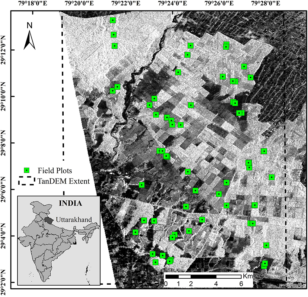
Figure 1. The ALOS-2/PALSAR-2 HH coherence amplitude image (scaled black for amplitude 0 and white for amplitude 1) of the Haldwani forest range is shown with the location of the field validation plots during field surveys in 2017-18. The extent of the TanDEM-X PolInSAR height is overlaid showing the common overlap region between ALOS-2/PALSAR-2 and TanDEM-X.

2.2. Field campaign

The field campaign in Haldwani was carried out for two major objectives - forest height and forest AGB estimation. The survey for forest height estimation was carried out in November 2015 and is explained in detail in Khati et al. (2017). The H₁₀₀ height is the mean of the tallest 100 trees in a 1 hectare (ha) plot, also called Lorey's height. For forest AGB mapping, the field campaign was carried out in March 2017 and November 2018. Field inventory data was collected for 60 field plots. Each plot is of 0.1 ha area (31.6 m × 31.6 m) and are generally established in homogeneous uni-species plantation compartments or mixed species compartments. For each plot, the trees with a diameter at breast height (dbh, 1.3 m above ground level) above 15 cm were considered for measurement. The dbh, height, species, and approximate age of each tree within a plot were measured with technical support from the State Forest Department. A total of 4,150 individual trees were surveyed during the two campaigns. Please note that the field measured AGB collected during campaigns in 2017 and 2018 (60 plots) is used in this study.

The AGB is defined “as the dry mass of live or dead matter from tree or shrub (woody plant) life forms, typically expressed as a per area density (e.g., Mg of aboveground biomass per hectare)” (Duncanson et al., 2022). The following steps detail the process used to estimate the field measured biomass.

1. The volume of each tree is computed using the site- and species-specific volumetric equations given by the Forest Survey of India (1996). The input to these equations is the dbh of the tree.

2. Next, using the wood density information from the Forest Survey of India, the volume is converted to biomass for each tree.

3. Finally, the biomass is aggregated for the 0.1 ha plot to obtain the AGB for the plot. This is then scaled accordingly to get the AGB in Mg/ha.

Following are the volumetric equations for the major species in the Haldwani test site as provided in the Forest Survey of India (1996). In these equations, V is the volume of the tree and D is the dbh of the tree. Using these equations, the tree volume is computed. The wood density is 0.4 for Poplus sp., 0.697 for Eucalyptus sp., 0.825 for Acacia catechu, 0.57 for Tectona grandis, 0.825 for Senegalia catechu, and 0.692 for Dalbergia sisoo.

$\begin{array}{l}V={(-0.143393+(3.040067*D))}^2\hfill \\ Poplussp.\hfill \\ V=0.02894-(0.89284*D)+(8.72416*D^2)\hfill \\ Eucalyptussp.\hfill \\ V=0.02384-(0.72161*D)+(7.46888*D^2)\hfill \\ Acaciacatechu\hfill \\ V=(0.08847-(1.46936*D)+(11.98979*D^2)\hfill \\ +(1.97056*D^3))*1.34\hfill \\ Tectonagrandis\hfill \\ V=(0.02384-(0.72161*D)+(7.46888*D^2))\hfill \\ Senegaliacatechu\hfill \\ V={(-0.3238+(3.0077*D))}^2\hfill \\ Dalbergiasisoo\hfill \end{array}$

It is to be noted that the field AGB calculations utilize volumetric equations which do not involve stand height (H₁₀₀) but only dbh. The potential for accurate field AGB measurement using allometric equations which use field measured H₁₀₀ and dbh have been highlighted in many studies (Feldpausch et al., 2011, 2012; Chave et al., 2014). However, for the Haldwani test site, allometric equations are not available for many species. Hence, volumetric equations are utilized.

The field measured AGB varies from 3.76 to 310 Mg/ha with a mean of 123 Mg/ha. The measured height at plot level was converted to H₁₀₀ height using the tallest 10 trees in a 0.1 ha area (see Khati et al., 2017, 2018). Figure 2 shows the field AGB as a function of H₁₀₀, the number of trees per plot, and average age of each plot. The coefficient of determination (R²) and mean squared error (MSE) for a logarithmic regression fit are also shown in Figure 2. As expected, the height and age are positively correlated with field measured AGB, while the number of trees decreases for high AGB plots.

FIGURE 2

Figure 2. Field campaign statistics: Forest mensuration height H₁₀₀, trees per plot, and the average age of the plot are shown as a function of field measured AGB. The coefficient of determination (R²) and Mean Squared Error (MSE) for a logarithmic regression between field measured AGB and the parameters on the ordinate are also shown in the plots.

2.3. Satellite data

2.3.1. ALOS-2/PALSAR-2 SAR data

Over Haldwani, L-band ALOS-2/PALSAR-2 fully polarimetric SAR data was acquired on five different dates in 2017: 19 March, 02 April, 16 April, 30 April, and 11 June. All the data were acquired in ascending pass at midnight (18:39 h UTC or 00:09 h local time) during the Indian summer. The range and azimuth spacing for all the acquisitions are 2.8 m and 3.2 m, respectively. The temperature and precipitation data are available from the nearest weather station at Pantnagar airport (located at the southern border of the Haldwani forest). The acquisition and weather details for the five acquisitions are detailed in Table 1. The cumulative precipitation at 3 h intervals before the acquisitions show that light rains were measured for two acquisitions (19 April and 30 April) while the weather for the remaining three acquisitions remains dry. Field work was carried out during the acquisition on 19/20 March 2017, which also confirms light moisture observed during the acquisition.

TABLE 1

Table 1. The ALOS-2/PALSAR-2 and TanDEM-X SAR data utilized over the test site.

2.3.2. TanDEM-X data, DEM, and Forest height

Three TerraSAR-X/TanDEM-X fully polarimetric PolInSAR data sets were acquired between December 2014 and March 2015. These data acquisition details are shown in Table 1 and have been discussed in detail in Khati et al. (2017). In this work, the PolInSAR inverted forest stand height from three PolInSAR acquisitions are used as a data product. Here, we briefly present the process followed. For detailed methodology, process work-flow, and analysis of the TanDEM-X PolInSAR data, refer to Khati et al. (2017, 2018). The PolInSAR data is radiometrically calibrated and corrected for SNR decorrelation. A modified three-stage inversion technique is utilized (Cloude, 2006) for forest height inversion. The retrieved forest stand height is validated using field measured H₁₀₀ heights from 0.1 ha plots. The PolInSAR height estimated from the acquisitions on 09 December 2014, 02 Feb 2015 and 13 Feb 2015 are used in this analysis. These are chosen as they show the best correlation with field measured H₁₀₀. The PolInSAR height maps (H_TDXn where n = 1, 2, 3) represent the stand height in meters above the local ground level.

The major objective of the TanDEM-X mission was to generate high-resolution global DEMs (Krieger et al., 2007). Recently, 90 m TanDEM-X DEM was released and is freely accessible. Furthermore, we have access to higher resolution of 12 m DEM as well. The DEMs are generated using multiple TanDEM-X VV-pol InSAR acquisitions. The InSAR phase centers are converted to elevations for DEM generation. For X-band, the microwave penetration through the vegetation canopy is limited and the phase center lies above the true ground. This introduces a vegetation bias in the generated DEM. We utilized the 12 m and 90 m DEM to generate a DTM. The DTM removes the vegetation bias from the DEM giving true-ground elevation. A mask of the non-forest region was generated using vegetation-free points obtained from multiple sources—field campaign, road and rail network, urban and agricultural fields, and non-forest pixels inside the forest range. The state forest department provided a non-forest region mask inside the forest range which includes small hamlets, roads, dirt tracks, and grasslands. Care was taken to ensure that the generated mask included well distributed points covering the entire forest range and surroundings. This mask was used with the 12 m DEM to generate the DTM using interpolation. The same set of points was also used to generate a 90 m DTM using the 90 m DEM. The difference in elevations between DTM and DEM provides the vegetation bias height for X-band SAR data. This vegetation bias is considered here as a pseudo-forest stand height, denoted in the text as H_TDM12 and H_TDM90 for the height estimated using the 12 m DEM/DTM and 90 m DEM/DTM, respectively. Thus, five different heights are used: three PolInSAR forest stand heights and two TanDEM-X estimated pseudo heights.

To assess the PolInSAR and TanDEM heights, the H₁₀₀ measured during the field campaign for 60 field plots are used. Figures 3a–e show the validation plots for PolInSAR heights H_TDXn and TanDEM-X heights. It is seen that the H_TDXn has a high correlation with H₁₀₀ (R² between 0.78 and 0.90). The variation is due to different baselines between the TerraSAR-X and TanDEM-X acquisitions. The TanDEM PolInSAR acquisition on 09 Dec 2014 (H_TDX2) showed the highest correlation with H₁₀₀. From Figures 3d,e, it is seen that the vegetation bias height estimated from 12 m (H_TDM12m) and 90 m (H_TDM90m) TanDEM-X DEM are positively correlated with H₁₀₀. This is expected since with increasing forest height, the vegetation bias should also increase. The R² is 0.68 and 0.63 for the 12 and 90 m DEMs, respectively. It is interesting to see that the loss of resolution does not have a drastic impact on the vegetation bias height estimation. The correlation between the H_TDM12m and H_TDM90m is shown in Figure 3f. Furthermore, Figure 4 provides a qualitative estimate of the forest height estimated using PolInSAR data (H_TDX2) and the 12 m TanDEM-X DEM. The variation of height in the forest range is well captured by the H_TDM12m.

FIGURE 3

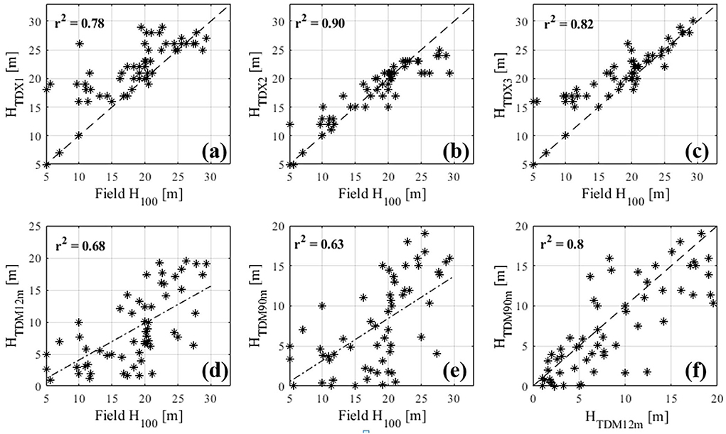
Figure 3. Height validation plots: The field estimated forest stand height (H₁₀₀) is plotted against PolInSAR estimated forest height for the three PolInSAR acquisitions (a–c), and vegetation bias height estimated using TanDEM-X 12 m DEM (d) and TanDEM-X 90 m DEM (e). In (f) the vegetation bias estimated from TanDEM-X 12 m DEM and TanDEM-X 90 m DEM are cross-validated. r² represents the coefficient of determination. The dotted line is the linear-fit line.

FIGURE 4

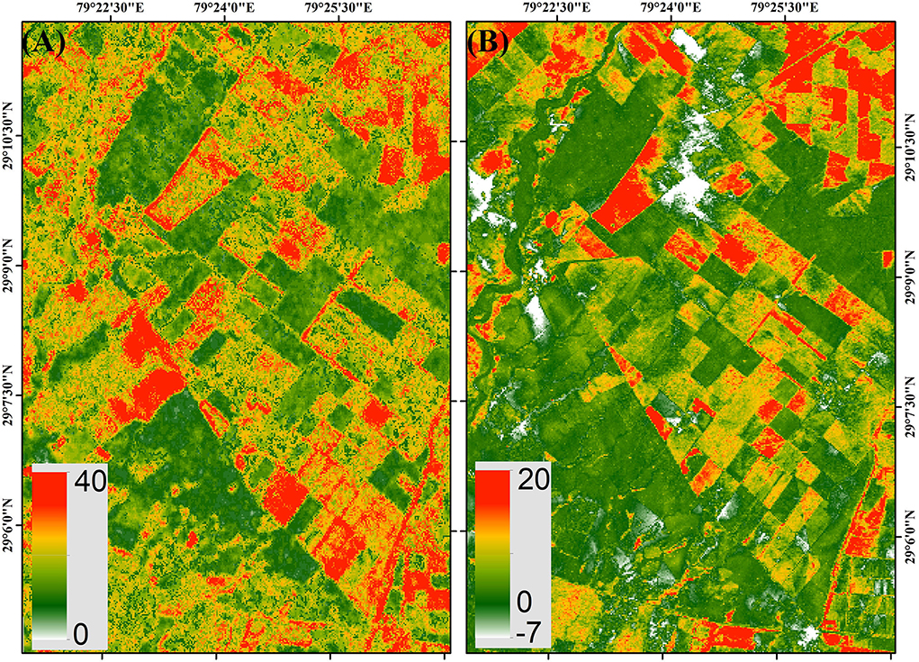
Figure 4. (A) TanDEM-X PolInSAR estimated height (in meters) map using the data acquired on 09 Dec 2014. (B) Vegetation bias height estimated from the difference between 12 m TanDEM-X DEM and the interpolated DTM.

2.4. Radar data processing

The ALOS-2/PALSAR-2 data is acquired in fine resolution quad-polarized strip-map mode and provided in single look complex (SLC) format. The data is radiometrically calibrated (Shimada et al., 2009; Englhart et al., 2011) and co-registered using the orbit parameters and the high resolution 12 m TanDEM-X DEM. The co-registered data sets are georeferenced and multi-looked to generate 30 m× 30 m pixels and to reduce speckle. The backscatter measured here is σ⁰ in slant range geometry. Using the 12 m TanDEM-X DEM and acquisition geometry, the local incidence angle (θ_i) for each pixel was estimated. It is generally observed that for rough forested regions, the σ⁰ backscatter has residual dependence on the local incidence angle (Soja et al., 2013) and therefore, backscatter in ground range γ⁰ is preferred. It is generated using

$\begin{array}{ll}{\gamma }_{PQ}^0=\frac{{\sigma }_{PQ}^0}{cos{\theta }_i}& (1)\end{array}$

where, PQ is the polarization observed - HH, HV, VV, or its Pauli combinations in HH+VV and HH-VV. The γ⁰ backscatter corrects the data for any topographic effects on the SAR signal.

2.5. Relating SAR data to forest AGB

2.5.1. ALOS-2/PALSAR-2 backscatter and AGB

The relation between SAR backscattering coefficients γ⁰, PolInSAR, and TanDEM-X DEM height with AGB are evaluated in this section. Figure 5 shows the relation between γ⁰ backscatter in HH, HV, and VV as a function of forest AGB. The backscatter ratios (HH/VV, HV/HH, and HV/VV) were evaluated and had a very weak relation with AGB. The backscatter-AGB relation is shown for the five ALOS-2/PALSAR-2 acquisitions. As seen in Table 1, the weather conditions differ between the acquisitions. To compensate for any extreme weather conditions, a temporally averaged backscatter coefficient is generated (shown in Figure 5 by blue squares) (Englhart et al., 2011). With multiple acquisitions, the temporal stability and utility of temporally averaged backscatter for AGB estimation can be evaluated.

FIGURE 5

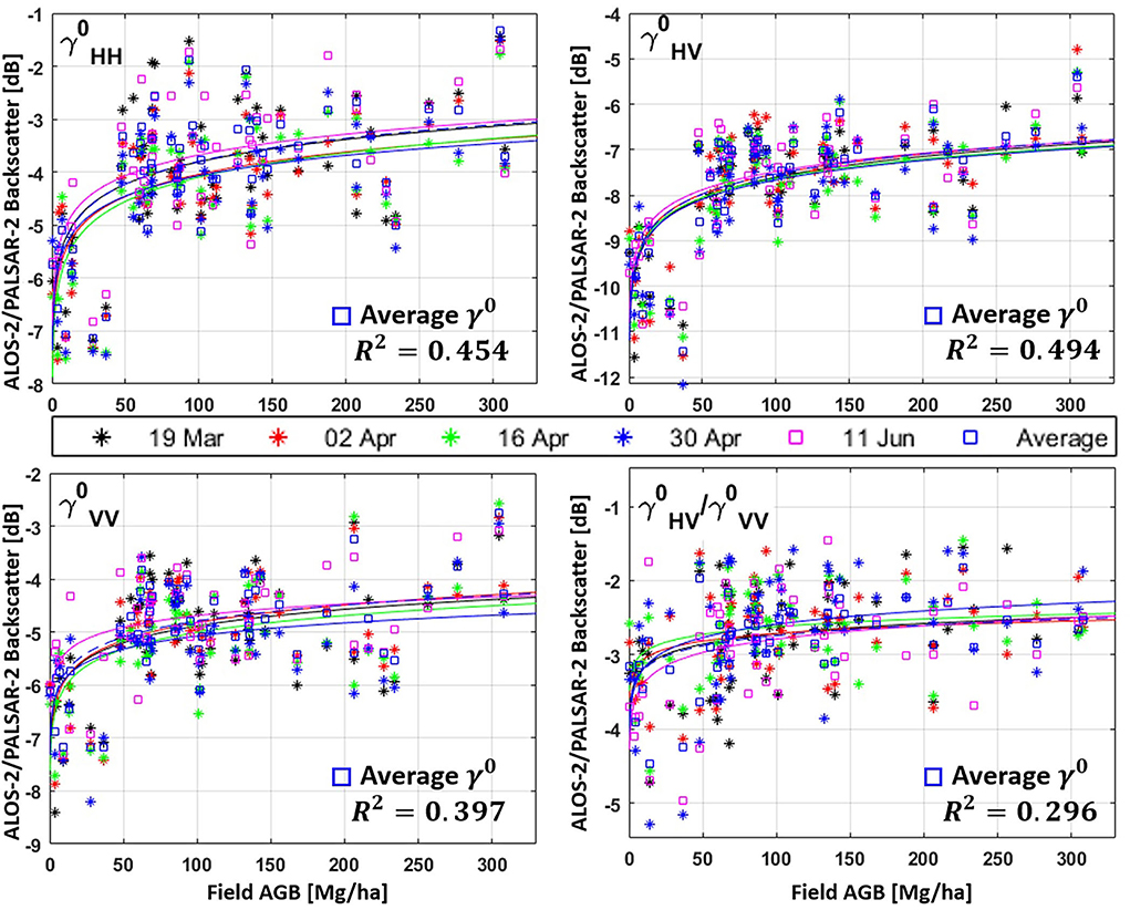
Figure 5. Gamma nought γ₀ backscatter for HH, HV, VV, and HV/VV backscatter ratio plotted (in dB) as a function of field measured AGB (Mg/ha). The running average trend is also plotted to simplify the analysis. Different colors correspond to the five ALOS-2/PALSAR-2 acquisitions and one temporal average backscatter. The coefficient of determination R² for the temporal average bacskcatter plot is also shown.

The backscatter-AGB saturation is estimated based on the method suggested by Watanabe et al. (2006) where the saturation threshold is identified as the slope where the backscatter-AGB slope approaches 0.01 dB per Mg/ha (for every 1 Mg/ha increase of AGB, the backscatter change is 0.01 dB). Using this technique, the backscatter-AGB curve saturates around 105 Mg/ha (for HH-polarization).

2.5.1.1. Forest height and AGB

In Figure 6, the variation of PolInSAR estimated height and TanDEM-X DEM estimated height as a function of AGB is plotted. Both the PolInSAR height and DEM/DTM height show a good correlation with AGB; however, there is higher variance in the case of DEM/DTM height.

FIGURE 6

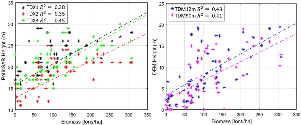
Figure 6. Relation between PolInSAR height (left) and DEM estimated height (right) as a function of AGB. The PolInSAR heights are estimated from three TanDEM-X acquisitions and DEM estimated heights are from 12 and 90 m TanDEM-X Global DEM and interpolated DTM. Dashed lines are the least-squares estimated best-fit lines.

From Figures 5, 6, the following observations can be made:

• All three polarizations (HH, HV, and VV) are well correlated with AGB for all acquisitions (Figure 5).

• Ratios of HH/VV and HV/HH are not correlated with AGB while HV/VV shows a weak relation (Figure 5).

• Temporal variation of backscatter is highest for HH-polarization and lowest for HV-polarization backscatter (Figure 5).

• PolInSAR and DEM estimated heights are related to AGB although the variance is high (Figure 6).

2.6. Forest AGB retrieval methods

2.6.1. Regression models

We utilize simple linear regression models to relate γ⁰ backscatter and estimated forest height with AGB. We first define the convention used in this paper:

1. ${\widehat{B}}_{Mn}$ is the biomass measured in Mg/ha using the Mn model

2. ${Ŵ}_{Mn}=lo{g}_e({\widehat{B}}_{Mn})$ is the natural logarithm of AGB estimated

3. ${\gamma }_{PQ}^0$ is the ground range, terrain corrected backscatter in PQ polarization measured in dB

4. H_TDXn is the PolInSAR forest height in meters estimated using one of the three TanDEM-X PolInSAR acquisitions

5. H_TDM12m and H_TDM90m is the forest height estimated using the 12 m and 90 m TanDEM-X global DEM as explained in Section 2.3.2.

Multiple combinations of backscatter in various polarizations and with different forest heights were evaluated to estimate forest AGB. A few among these which provide interesting observations and are consistent in AGB estimation for all five ALOS-2/PALSAR-2 data are discussed here. We start with a simple model relating the cross-polarized backscatter to AGB (Le Toan et al., 2011; Sandberg et al., 2011; Soja et al., 2013).

$\begin{array}{ll}{Ŵ}_{M1}=a_0+a_1\left[{\gamma }_{HV}^0\right]& (2)\end{array}$

where a₀ and a₁ are the model parameters. Following the analysis in Section 2.5.1 and observations in Figure 5, co-polar channels also have a good correlation with AGB. The next two models add the co-polar channels to obtain a linear regression model which utilizes the complete polarimetric information (Rignot et al., 1995; Saatchi et al., 2007, 2011; Sandberg et al., 2011).

$\begin{array}{ll}{Ŵ}_{M2}=a_0+a_1\left[{\gamma }_{HV}^0\right]+a_2\left[{\gamma }_{HH}^0\right]& (3)\end{array}$

$\begin{array}{ll}{Ŵ}_{M3}=a_0+a_1\left[{\gamma }_{HV}^0\right]+a_2\left[{\gamma }_{HH}^0\right]+a_3\left[{\gamma }_{VV}^0\right]& (4)\end{array}$

These models utilize simple first order parameters of radar backscatter. In Saatchi et al. (2007), the WCM model is simplified into a quadratic form of the equation. The quadratic model mimics the loss of sensitivity of backscatter for higher biomass and is also used as a reference model by Soja et al. (2013). We evaluate this model to assess it with respect to M3. The model is given by

$\begin{array}{ll}{Ŵ}_{M4}=a_0+a_1\left[{\gamma }_{HV}^0\right]+a_2{\left[{\gamma }_{HV}^0\right]}^2+a_3\left[{\gamma }_{HH}^0\right]+a_4{\left[{\gamma }_{HH}^0\right]}^2+a_5\left[{\gamma }_{VV}^0\right]+a_6{\left[{\gamma }_{VV}^0\right]}^2.& (5)\end{array}$

M1 to M4 provide different linear models which estimate AGB as a function of SAR backscatter. The estimated forest stand height is next evaluated for its utility in AGB estimation. We start with a simple linear model relating the estimated forest stand height with AGB

$\begin{array}{ll}{Ŵ}_{M5}=a_0+a_1\left[H_X\right]H_X=H_{TDXn},H_{TDM12m}or{H}_{TDM90m}& (6)\end{array}$

Next, the L-band backscatter is combined with height to assess a combined model. The cross-pol and co-pol backscatter is added in steps to assess any incremental improvement with multi-polarimetric data.

$\begin{array}{ll}{Ŵ}_{M6}=a_0+a_1\left[H_X\right]+a_2\left[{\gamma }_{HV}^0\right]& (7)\end{array}$

$\begin{array}{ll}{Ŵ}_{M7}=a_0+a_1\left[H_X\right]+a_2\left[{\gamma }_{HV}^0\right]+a_3\left[{\gamma }_{HH}^0\right]& (8)\end{array}$

$\begin{array}{ll}{Ŵ}_{M8}=a_0+a_1\left[H_X\right]+a_2\left[{\gamma }_{HV}^0\right]+a_3\left[{\gamma }_{HH}^0\right]+a_4\left[{\gamma }_{VV}^0\right]& (9)\end{array}$

3. Results and discussion

In this section, the overall methodology followed is explained, and the models are evaluated for their performance and discussed. Figure 7 shows the overall methodology followed. The training and validation samples are common across all the acquisitions. Only those field plots which are covered by ALOS-2/PALSAR-2 and TanDEM-X acquisitions are used.

FIGURE 7

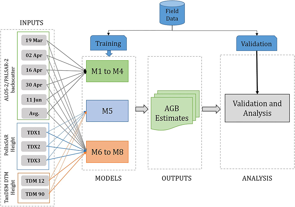
Figure 7. Relation between PolInSAR height (left) and DEM estimated height (right) as a function of AGB. The PolInSAR heights are estimated from three TanDEM-X acquisitions and DEM estimated heights are from 12 m and 90 m TanDEM-X Global DEM and interpolated DTM.

In regression modeling, the selection of training samples with high accuracy and low bias is important (Soja et al., 2013). The field campaign estimated forest AGB is accurate and used for training and validation. These multivariate regression models are trained on 24 randomly selected samples from the 60 field plots. The validation is carried out on the remaining 36 field plots. The training and validation plots represent the complete range of AGB values from 4 to 310 Mg/ha. Further to test cross-validity and temporal model stability, we train the model using the backscatter of one acquisition and validated using the backscatter of another (Soja et al., 2013). To verify the model validation, two parameters are evaluated for each model:

• Root mean square error (RMSE):

$\begin{array}{ll}RMSE=\sqrt{\frac{1}{N}{\displaystyle \sum _i}\widehat{R}{(i)}^2}& (10)\end{array}$

where N is the number of observations. Note that i sweeps through all the 36 validation plots for each acquisition.

• Coefficient of determination R² is calculated for no-intercept models and is given as

$\begin{array}{ll}{R}^2=1-\frac{{\displaystyle {\sum }_i{({\widehat{B}}_{field}(i)-{\widehat{B}}_M(i))}^2}}{{\displaystyle {\sum }_i{({\widehat{B}}_{field}(i)-{\overline{B}}_{field})}^2}}& (11)\end{array}$

where ${\widehat{B}}_{field}$ is the biomass measured during the field campaign, ${\widehat{B}}_M$ is the model estimated biomass, and ${\bar{B}}_{field}$ represents the mean field measured biomass (i.e., mean biomass of all plots).

3.1. Temporal model validation

The models are co-validated and cross-validated. In co-validation, the model is trained and validated using backscatter from the same acquisition (date) data set. Whereas in cross-validation, the models are trained using one L-band acquisition backscatter data set and validated using data from other dates. Table 2 shows the training and validation dates for all models except M5. Model M5 is not analyzed since it does not have backscatter as input (see Equation 6). In Table 2, models M6 to M8 have TDX2 height as a common input. TDX2 is chosen since it has the highest accuracy with H₁₀₀ (see Figure 3). From initial analysis, it is observed that all the models consistently under-estimated biomass for plots with AGB > 250 Mg/ha. Since only 4 field plots have AGB above 250 Mg/ha we do not expect significant performance deterioration.

TABLE 2

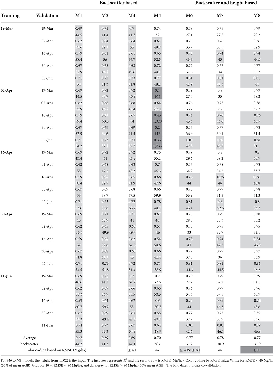
Table 2. Temporal validation: Results of validation carried out on Models M1 to M4 (backscatter based) and M6 to M8 (backscatter and height based).

In Table 2, all combinations of dates are examined and co- and cross-validation results are presented. The R² and RMSE are evaluated for each date pair and model. The RMSE ranges from a minimum of 27.2 Mg/ha (22% of mean AGB) to a maximum of 163 Mg/ha (135% of mean AGB). Two extreme results for cross-validation of M4 using 02-April data are excluded. For ease of interpretation, the RMSE values are used to color-code the validation table. The model dates for which RMSE is less than 40 Mg/ha (30% of mean AGB) are white and the worst performing model dates having RMSE greater than 80 Mg/ha (65% of mean AGB) are darkened. The remaining model date pairs are gray.

It is interesting to observe the performance of models with subsequently higher polarimetric information content. The polarimetric information content increases from M1 to M3. Model M4 is evaluated and compared with M3 as both have the same polarimetric inputs, but M4 has a quadratic form. On the right side of Table 2, M6–M8 have a common TDX2 input height. Overall, it is evident from Table 2 that the combined models with L-band backscatter and X-band height (M6–M8) input perform better than backscatter-only models.

Table 3 depicts the overall performance of the models across all L-band acquisitions. The mean RMSE and SD are calculated for co- and cross-validation cases. The values in brackets are %RMSE (% of mean AGB) for the models. M3 performs best among backscatter based models with an RMSE of 46.3 ± 6 Mg/ha or 37.7% of mean AGB. With the addition of height, the models with combined backscatter and height input (M6–M8) perform significantly better than backscatter-only models. The model inversion improves with RMSE reducing to 35.6 ± 8 Mg/ha or 29% of mean AGB for the M6 model. With the addition of HH-pol backscatter information in M7, the performance remains similar, while with VV-pol backscatter included in M8, the performance degrades.

TABLE 3

Table 3. Overall model performance for models M1 to M4 (backscatter based) and M6 to M8 (backscatter and height based).

For cross-validation, the performance varies for the models with RMSE ranging from 37.3 to 71 Mg/ha. M4 has the highest RMSE and has a very high variance. This is observed in Table 2 for model M4 trained with 02-April data and cross-validated for other dates where RMSE > 163 Mg/ha are observed. However, it seems to be an exception, since, for other training dates, M4 performs reasonably well with a mean RMSE of 56 Mg/ha (excludes extremes for 02-April training data). If these extreme results are ignored, then the cross-validation results have similar trends to co-validation results with M2 and M3 providing similar validation results in backscatter only models. In combined models, M6 has the best performance with an RMSE of 37.3 ± 8 Mg/ha or 30.1% of mean AGB. The model performance deteriorates for M7 and M8.

In summary, the cross-validation shows stable model performance for all models except M4. Among co- and cross-validation, the model performance does not deteriorate significantly (see Table 3). Single-pol model M1 performs poorly across all validation scenarios (RMSE 53.1 Mg/ha) while addition of polarimetric information in M2 (RMSE 48.5 Mg/ha) or PolInSAR information (height) in M6 (RMSE 37 Mg/ha) improves the model performance. From Table 2, it is observed that all models seem to perform better for the 19-March acquisition irrespective of the training date selected. For other training dates, the model performance is sensitive to what the validation dates are. This might be due to the gradual change of phenology from 19-March to April acquisitions. Although not common to all regions of the forest, the teak plantations gradually lose their leaves during March and are leaf-less during April. This might be a reason for better model inversion for 19-March data. The model performance for 19-March data with TDX2 height input across all models is shown in Figure 8. The validation plots show the improved accuracy with the M6 model and gradual improvement from M1 to M3.

FIGURE 8

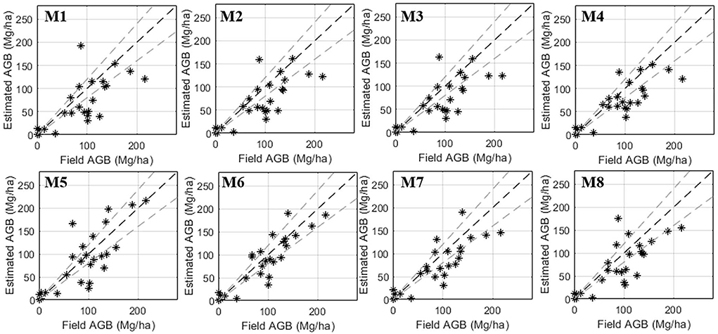
Figure 8. Comparison of the eight models with training and validation carried out using L-band backscatter from 19-March data and TDX2 height. First row represents models based on backscatter and second row represents combined models based on backscatter and height.

3.1.1. Model stability

The linear regression coefficients (a₀, a₁…) are estimated for the models at all L-band acquisition dates and all heights. The stability of the model can be assessed from the variations in these regression coefficients over time. A stable model is characterized by lower variations in the estimated coefficients over different acquisition times. Table 4 shows the mean and standard deviation of the model coefficients for the eight models. The models are evaluated for all the five L-band acquisitions for two height inputs of TDX2 and TDM90m. These two heights are selected as they represent two distinct sources of heights - TanDEM-X based PolInSAR height and TanDEM-X Global DEM based height (open source). The models coefficients for M5–M8 are tabulated for the two height inputs. Note that as M5 does not depend on backscatter input, only the mean is shown here.

TABLE 4

Table 4. Validation of combined models for all five heights and five L-band acquisitions.

In Table 4, a₀ is the intercept of the models. It is interesting to observe that a₀ is similar for M1 to M3 and M6 to M9 indicating a similar bias for bare ground regions (AGB≈ 0). M4 has the highest variability of estimated coefficients among all models indicating low model stability over a temporal span. M4 has a quadratic form and in general there is a very high variance for the squared components of the equation. Also, the coefficient a₄ ≈ 0 indicates the very low utility of the ${\left[{\gamma }_{HH}^0\right]}^2$ term in Equation (5).

Among the combined models (M6–M8), the variance of coefficients is lower compared to backscatter based models indicating higher stability over time. It is observed that both TDX2 and TDM90m perform reliably across all models.

3.2. Combined model validation

In this section, we discuss the proposed combined models where the backscatter (PolSAR) and height (PolInSAR) are utilized as inputs. From the results in the earlier section, it is clear that the addition of height leads to a better inversion performance when compared with multiple backscatter-only based models. Table 4 shows the validation performance of the four combined models M5 to M8 based on RMSE and R². The table is color coded based on RMSE with the same criteria as applied to Table 2 for ease of interpretation. For models M6 to M8, the inputs are height and backscatter. As M5 is based only on height, it is independent of L-band acquisition dates. M5, performs poorly with the RMSE ranging between 68.9 Mg/ha for TDX2 height and 134 Mg/ha for TDM90m height. With the addition of polarimetric information (in M6 to M8), the model performance improves. The improvement with the addition of cross-pol backscatter in M6 is significant. However, with further polarimetric parameters added, the improvement is not consistent across all acquisitions. The models perform best with the TDX2 height input (RMSE between 27.2 and 46.9 Mg/ha). The best inversion performance is observed for M6 model for 19-March backscatter data and TDX-2 height with RMSE of 27.1 Mg/ha (22% of mean AGB). Among the five L-band acquisitions, the acquisitions on 16-April and 11-June lead to lower inversion performance. Such variations can be due to weather parameters. However, no precipitation was recorded on 16-April while for 11-June data, light precipitation of 1.4 mm was recorded 6 h prior to acquisition (see Table 1). Thus, any change in soil moisture or dielectric properties does not explain the reduced inversion performance for both dates.

Among the PolInSAR acquisitions, the model's accuracy and height inversion accuracy are correlated. For TDX1, TDX2, and TDX3, the R² of height inversion are 0.78, 0.90, and 0.82, respectively (see Figure 3). Similarly, the trend in Table 5 shows that the average RMSE across all model-date pairs is 50.1 Mg/ha, 39.2 Mg/ha, and 42.2 Mg/ha for TDX1, TDX2, and TDX3, respectively. Thus, the accuracy of utilized height in the proposed model is critical for accurate AGB modeling.

TABLE 5

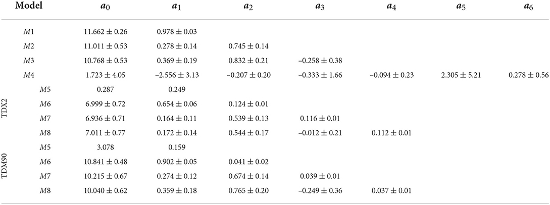
Table 5. Mean and standard deviation of model coefficients for the eight models evaluated across multiple dates for TDX2 height and TDM90m height inputs.

For the pseudo-heights (or vegetation bias heights) estimated using the TanDEM-X DEM/DTM height difference, we observe a rather interesting trend. The models with TDM12m and TDM90m heights have higher RMSE compared to PolInSAR height models as expected. However, among the two DEMs, the pseudo-height estimated from TDM90m performs better than TDM12m. For TDM90m, the mean RMSE for M6 to M8 models across all dates is 55.5 Mg/ha, while that for TDM12m is 56.4 Mg/ha. It seems that the 90 m DEM estimated vegetation bias height is more reflective of the trend in H₁₀₀ height.

The temporal average backscatter from all the five L-band acquisitions is also used to model the AGB. It is observed that average backscatter leads to improved validation results for all the models. Figure 9 shows the validation plots for M5 to M8 with temporally averaged backscatter as input and evaluated for TDX2 and TDM90m heights. These models have inversion results with RMSE below 40 Mg/ha. The best accuracy is observed for the M8 model with TDX2 PolInSAR height (29.8 Mg/ha or 24.3%) and TDM90m DEM/DTM height (32.7 Mg/ha or 26.6%). The variations in backscatter due to changes in weather, soil moisture, and possibly phenology is reduced with temporal averaging, providing better AGB inversion.

FIGURE 9

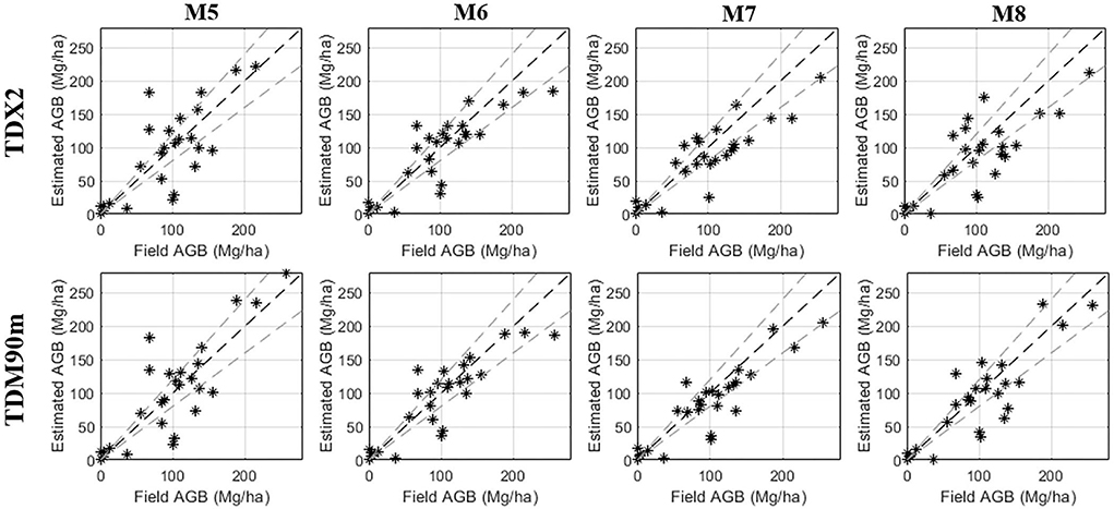
Figure 9. Comparison of combined models based on backscatter and height. Training and validation carried out using temporally averaged backscatter data. First row represents models with TDX2 PolInSAR height as input and second row represents models with TDM90m DEM estimated height as input.

3.3. AGB mapping and model stability

3.3.1. Mapping the biomass of the Haldwani forest

In this section, the models are applied to the data and biomass maps are generated for qualitative analysis. Figure 10 shows the AGB maps (Figures 10A–G) along with a RGB map (Figure 10H) generated using the general four component (G4U) decomposition (Singh et al., 2013) for ease of interpretation. The G4U scattering power decomposition with unitary transformation of coherency matrix utilizes 100% of the scattering information content of the coherence matrix. Double unitary transformations are implemented in the G4U method that corrects polarization orientation shifts and subsequently takes into account all the elements of the coherence matrix T for decomposition. The input T is expanded into four sub-matrices:

$T=f_s{T}_{surface}+f_d{T}_{double}+f_v{T}_{volume}+f_c{T}_{helix}$

FIGURE 10

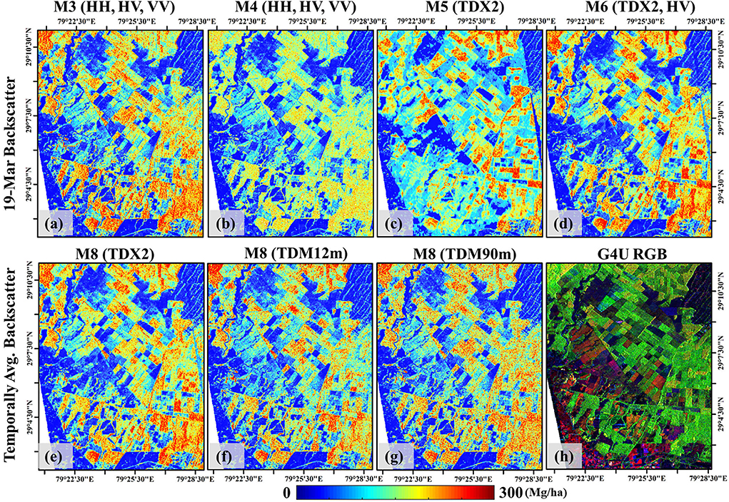
Figure 10. AGB maps generated for different models. (A,B) are AGB maps generated using M3 and M4 models for L-band data acquisition on 19-March. (C) utilizes the M5 model with the TDX2 height as input, whereas (D) shows the AGB map using the M6 model for 19-March data and TDX2 height. (E–G) represents maps for M8 model which utilize the temporally averaged backscatter as input with TDX2, TDM12m and TDM90m heights respectively. The G4U RGB image is shown in (H) for visual reference. Here the dihedral scattering, volume scattering and surface scattering are represented by red, green and blue colors respectively.

T_surface, T_double, T_volume, and T_helix represent the four types of scattering mechanisms - surface, double-bounce, volume, and helix, respectively. The volume scattering T_volume can be expressed in either of the four volume scattering distributions models, uniform distribution, cosine distribution, sine distribution, and volume scattering caused by oriented dihedral scatterers as explained in detail by Singh et al. (2013). The nature of the volume matrix is optimized for each pixel. The total power is divided into surface scattering power P_s, double-bounce scattering power P_d, volume scattering power P_v, from dipole and/or oriented dihedral, and helix P_c accordingly. In Figure 10H, the RGB image is generated using the P_d, P_v, and P_s for the red, green and blue channels, respectively.

The first row (Figures 10A–D) shows AGB maps generated for different models based on 19-March L-band backscatter data. The bottom row (Figures 10E–G) shows maps generated using the M8 model with a common input of temporally averaged backscatter and the height from TDX2 (e), TDM12m (f), and TDM90m (g).

Among the seven models shown in Figure 10, M6 (Figure 10D) has the highest accuracy with an RMSE of 27.1 Mg/ha (22% of mean AGB) and an R² of 0.78 (refer to Table 2). Since the main objective of this paper is to explore the potential of combining backscatter and height information for AGB mapping this AGB map is utilized as a reference for qualitative analysis. Models M3 and M4 utilize the backscatter information of three polarimetric channels. However, M4 under-estimates the forest AGB as seen in Figure 10B. The model performs well for low-AGB plantations while under-estimating dense-AGB regions. As M4 utilizes quadratic regression, a possible explanation for under-estimation can be over-fitting. M5 (Figure 10C) and M6 (Figure 10D) utilize TDX2 height as a common input. Height-based model M5 has poor inversion performance (RMSE of 68.9 Mg/ha) and shows the low variance in the AGB map. Comparatively, adding cross-pol backscatter to TanDEM-X forest height shows improvement in AGB modeling (see Figure 10D). For model M8 (Figures 10E–G), the RMSE for the three height inputs TDX2, TDM12m, and TDM90m are 29.8 Mg/ha, 40.3 Mg/ha, and 32.7 Mg/ha, respectively. The models with TDM12m and TDM90m heights over-estimate the low-AGB forest regions. The forest AGB map generated using TDM90m accurately represents the biomass variation within the forest but loses out on finer details due to coarse resolution.

4. Conclusions

In this paper, new biomass estimation models which combine L-band polarimetric SAR backscatter from ALOS-2/PALSAR-2 and PolInSAR height from TanDEM-X are presented and validated over an Indian managed tropical forest. The AGB maps generated from these models are shown in Figure 10. The combined models perform significantly better than previously published backscatter based models with a 19% to 46% improvement in accuracy. The combined models can estimate AGB reliably up to 250 Mg/ha. Among the models evaluated, a combination of temporally averaged L-band backscatter and TDM90m height leads to accurate AGB estimation (RMSE = 27% of mean AGB). These results are motivating as the open source 90 m TanDEM DEM data combined with ALOS-2/PALSAR-2 backscatter data has the potential to be applied over extended regions. Furthermore, the sensitivity of L-band SAR backscatter for low AGB (<100 Mg/ha) retrieval is shown in this study. This complements the work done by Ningthoujam et al. (2018) using L-band ALOS PALSAR data on another Indian tropical forest. The combined models are temporally stable, which is necessary for AGB-change mapping. The method of vegetation bias height estimation using DEM/DTM needs to be explored further.

The two upcoming SAR missions (L- and S-band NISAR and P-band BIOMASS) have dedicated ecosystem objectives for AGB retrieval. Some studies have predicted S-band sensitivity to forest AGB<100 Mg/ha based on a modeling framework across different tropical forests (Ningthoujam et al., 2016, 2017). It seems that the NISAR mission would be suitable for low AGB (<100 Mg/ha) mapping and the BIOMASS mission for dense AGB (>100 Mg/ha) retrieval, keeping view of temporal and ionospheric properties (Quegan et al., 2019). The approach in this paper can be useful to improve the potential of L- and S-band SAR data for AGB mapping above 100 Mg/ha. As part of further work, an automated process of identification of bare ground regions using optical and SAR data should be developed and the combined models should be tested across other tropical test sites.

Data availability statement

The data analyzed in this study is subject to the following licenses/restrictions: The distribution of SAR and field raw data supporting the conclusion of this study is restricted because of project agreements between the authors and the data providers. Requests to access these datasets should be directed to unmesh.khati@iiti.ac.in, gulab.singh@iitb.ac.in.

Author contributions

UG conceptualized the overall methodology, collected the field data, processed the satellite data, analyzed the results, and wrote the manuscript. GS provided access to the data, secured the funding and support in reviewing and editing the manuscript. All authors contributed to the article and approved the submitted version.

Acknowledgments

The authors would like to thank the German Aerospace Center (DLR) for the TanDEM-X acquisitions and TanDEM 12 m DEM under the Science Phase AO Project No. NTI_POLI_6937 and DEM_GLAC1805. The authors thank the Japanese Space Exploration Agency (JAXA) for fully polarimetric ALOS-2/PALSAR-2 data under Project No. JAXA-1396 and JAXA-3055. The authors are grateful to the reviewers for their constructive comments. The authors would also like to thank the Uttarakhand State Forest Department for technical support during field campaigns.

Conflict of interest

The authors declare that the research was conducted in the absence of any commercial or financial relationships that could be construed as a potential conflict of interest.

Publisher's note

All claims expressed in this article are solely those of the authors and do not necessarily represent those of their affiliated organizations, or those of the publisher, the editors and the reviewers. Any product that may be evaluated in this article, or claim that may be made by its manufacturer, is not guaranteed or endorsed by the publisher.

References

Askne, J. I., Soja, M. J., and Ulander, L. M. (2017). Biomass estimation in a boreal forest from TanDEM-X data, lidar DTM, and the interferometric water cloud model. Remote Sens. Environ. 196, 265–278. doi: 10.1016/j.rse.2017.05.010

CrossRef Full Text | Google Scholar

Avtar, R., Suzuki, R., and Sawada, H. (2014). Natural forest biomass estimation based on plantation information using PALSAR data. PLoS ONE 9, e86121. doi: 10.1371/journal.pone.0086121

PubMed Abstract | CrossRef Full Text | Google Scholar

Behera, M., Tripathi, P., Mishra, B., Kumar, S., Chitale, V., and Behera, S. K. (2016). Above-ground biomass and carbon estimates of shorea robusta and tectona grandis forests using QuadPOL ALOS PALSAR data. Adv. Space Res. 57, 552–561. doi: 10.1016/j.asr.2015.11.010

CrossRef Full Text | Google Scholar

Cartus, O., Santoro, M., Wegmüller, U., and Rommen, B. (2019). Benchmarking the retrieval of biomass in boreal forests using p-band sar backscatter with multi-temporal c- and l-band observations. Remote Sens. 11, 1695. doi: 10.3390/rs11141695

CrossRef Full Text | Google Scholar

Chave, J., Réjou-Méchain, M., Búrquez, A., Chidumayo, E., Colgan, M. S., Delitti, W. B., et al. (2014). Improved allometric models to estimate the aboveground biomass of tropical trees. Glob. Chang Biol. 20, 3177–3190. doi: 10.1111/gcb.12629

PubMed Abstract | CrossRef Full Text | Google Scholar

Cloude, S. R. (2006). Polarization coherence tomography. Radio Sci. 41, 1–27. doi: 10.1029/2005RS003436

CrossRef Full Text | Google Scholar

Dobson, M., Ulaby, F., LeToan, T., Beaudoin, A., Kasischke, E., and Christensen, N. (1992). Dependence of radar backscatter on coniferous forest biomass. IEEE Trans. Geosci. Remote Sens. 30, 412–415. doi: 10.1109/36.134090

CrossRef Full Text | Google Scholar

Duncanson, L., Armston, J., and Disney, M. (2022). Ceos Land Product Validation Subgroup. Available online at: https://lpvs.gsfc.nasa.gov/AGB/AGB_home.html (accessed June 6, 2022).

Google Scholar

Englhart, S., Keuck, V., and Siegert, F. (2011). Aboveground biomass retrieval in tropical forests–The potential of combined X- and L-band SAR data use. Remote Sens. Environ. 115, 1260–1271. doi: 10.1016/j.rse.2011.01.008

CrossRef Full Text | Google Scholar

Feldpausch, T. R., Banin, L., Phillips, O. L., Baker, T. R., Lewis, S. L., Quesada, C. A., et al. (2011). Height-diameter allometry of tropical forest trees. Biogeosciences 8, 1081–1106. doi: 10.5194/bg-8-1081-2011

CrossRef Full Text | Google Scholar

Feldpausch, T. R., Lloyd, J., Lewis, S. L., Brienen, R. J. W., Gloor, M., Monteagudo Mendoza, A., et al. (2012). Tree height integrated into pantropical forest biomass estimates. Biogeosciences 9, 3381–3403. doi: 10.5194/bg-9-3381-2012

CrossRef Full Text | Google Scholar

Forest Survey of India (1996). Volume Equations for Forests of India, Nepal, and Bhutan. Dehradun: Forest Survey of India, Ministry of Environment & Forests, Government of India.

Fransson, J. E. S. (1999). Estimation of stem volume in boreal forests using ers-1 c- and jers-1 l-band sar data. Int. J. Remote Sens. 20, 123–137. doi: 10.1080/014311699213640

CrossRef Full Text | Google Scholar

Ghasemi, N., Sahebi, M. R., and Mohammadzadeh, A. (2011). A review on biomass estimation methods using synthetic aperture radar data. Int. J. Geomat. Geosci. 1, 13. doi: 10.1/1/372/9870

CrossRef Full Text | Google Scholar

Henderson, F., and Lewis, A. (1998). Principles and Applications of Imaging Radar. Manual of Remote Sensing:3rd Edn, Vol. 2. New York, NY: John Wiley and Sons.

Google Scholar

Hoekman, D., and Quiriones, M. (2000). Land cover type and biomass classification using AirSAR data for evaluation of monitoring scenarios in the Colombian Amazon. IEEE Trans. Geosci. Remote Sens. 38, 685–696. doi: 10.1109/36.841998

CrossRef Full Text | Google Scholar

Imhoff, M. (1993). “Radar backscatter/biomass saturation: observations and implications for global biomass assessment,” in Proceedings of IGARSS '93-IEEE International Geoscience and Remote Sensing Symposium (Tokyo: IEEE), 43–45.

Google Scholar

Joshi, N., Mitchard, E. T. A., Brolly, M., Schumacher, J., Fernández-Landa, A., Johannsen, V. K., et al. (2017). Understanding ‘saturationŠ of radar signals over forests. Scientific Rep. 7, 3505. doi: 10.1038/s41598-017-03469-3

PubMed Abstract | CrossRef Full Text

Khati, U., Lavalle, M., and Singh, G. (2019). Spaceborne tomography of multi-species Indian tropical forests. Remote Sens. Environ. 229, 193–212. doi: 10.1016/j.rse.2019.04.017

CrossRef Full Text | Google Scholar

Khati, U., Singh, G., and Ferro-Famil, L. (2017). Analysis of seasonal effects on forest parameter estimation of Indian deciduous forest using TerraSAR-X PolInSAR acquisitions. Remote Sens. Environ. 199, 265–276. doi: 10.1016/j.rse.2017.07.019

CrossRef Full Text | Google Scholar

Khati, U., Singh, G., and Kumar, S. (2018). Potential of space-borne PolInSAR for forest canopy height estimation over india–a case study using fully PolarimetricL-,C-, andX-Band SAR data. IEEE J. Select. Top. Appl. Earth Observat. Remote Sens. 11, 2406–2416. doi: 10.1109/JSTARS.2018.2835388

CrossRef Full Text | Google Scholar

Krieger, G., Moreira, A., Fiedler, H., Hajnsek, I., Werner, M., Younis, M., et al. (2007). TanDEM-X: a satellite formation for high-resolution SAR interferometry. IEEE Trans. Geosci. Remote Sens. 45, 3317–3341. doi: 10.1109/TGRS.2007.900693

CrossRef Full Text | Google Scholar

Kugler, F., Schulze, D., Hajnsek, I., Pretzsch, H., and Papathanassiou, K. P. (2014). TanDEM-X Pol-InSAR performance for forest height estimation. IEEE Trans. Geosci. Remote Sens. 52, 6404–6422. doi: 10.1109/TGRS.2013.2296533

CrossRef Full Text | Google Scholar

Kumar, S., Joshi, S. K., and Govil, H. (2017a). Spaceborne polsar tomography for forest height retrieval. IEEE J. Select. Top. Appl. Earth Observat. Remote Sens. 10, 5175–5185. doi: 10.1109/JSTARS.2017.2741723

CrossRef Full Text | Google Scholar

Kumar, S., Khati, U. G., Chandola, S., Agrawal, S., and Kushwaha, S. P. (2017b). Polarimetric SAR interferometry based modeling for tree height and aboveground biomass retrieval in a tropical deciduous forest. Adv. Space Res. 60, 571–586. doi: 10.1016/j.asr.2017.04.018

CrossRef Full Text | Google Scholar

Kuplich, T. M., Curran, P. J., and Atkinson, P. M. (2005). Relating SAR image texture to the biomass of regenerating tropical forests. Int. J. Remote Sens. 26, 4829–4854. doi: 10.1080/01431160500239107

CrossRef Full Text | Google Scholar

Le Toan, T., Beaudoin, A., Riom, J., and Guyon, D. (1992). Relating forest biomass to SAR data. IEEE Trans. Geosci. Remote Sens. 30, 403–411. doi: 10.1109/36.134089

CrossRef Full Text | Google Scholar

Le Toan, T., Quegan, S., Davidson, M., Balzter, H., Paillou, P., Papathanassiou, K., et al. (2011). The BIOMASS mission: mapping global forest biomass to better understand the terrestrial carbon cycle. Remote Sens. Environ. 115, 2850–2860. doi: 10.1016/j.rse.2011.03.020

CrossRef Full Text | Google Scholar

Liao, Z., He, B., Quan, X., van Dijk, A. I., Qiu, S., and Yin, C. (2019). Biomass estimation in dense tropical forest using multiple information from single-baseline P-band PolInSAR data. Remote Sens. Environ. 221, 489–507. doi: 10.1016/j.rse.2018.11.027

CrossRef Full Text | Google Scholar

Luckman, A., Baker, J., Honzák, M., and Lucas, R. (1998). Tropical forest biomass density estimation using JERS-1 SAR: seasonal variation, confidence limits, and application to image mosaics. Remote Sens. Environ. 63, 126–139. doi: 10.1016/S0034-4257(97)00133-8

CrossRef Full Text | Google Scholar

Luckman, A., Baker, J., Kuplich, T. M., da Costa Freitas Yanasse, C., and Frery, A. C. (1997). A study of the relationship between radar backscatter and regenerating tropical forest biomass for spaceborne sar instruments. Remote Sens. Environ. 60, 1–13. doi: 10.1016/S0034-4257(96)00121-6

CrossRef Full Text | Google Scholar

Mermoz, S., Réjou-Méchain, M., Villard, L., Le Toan, T., Rossi, V., and Gourlet-Fleury, S. (2015). Decrease of L-band SAR backscatter with biomass of dense forests. Remote Sens. Environ. 159, 307–317. doi: 10.1016/j.rse.2014.12.019

CrossRef Full Text | Google Scholar

Mitchard, E. T. A., Saatchi, S. S., Woodhouse, I. H., Nangendo, G., Ribeiro, N. S., Williams, M., et al. (2009). Using satellite radar backscatter to predict above-ground woody biomass: a consistent relationship across four different African landscapes. Geophys. Res. Lett. 36, 692. doi: 10.1029/2009GL040692

CrossRef Full Text | Google Scholar

Næsset, E., Gobakken, T., Solberg, S., Gregoire, T. G., Nelson, R., Ståhl, G., et al. (2011). Model-assisted regional forest biomass estimation using LiDAR and InSAR as auxiliary data: a case study from a boreal forest area. Remote Sens. Environ. 115, 3599–3614. doi: 10.1016/j.rse.2011.08.021

CrossRef Full Text | Google Scholar

Neumann, M., Saatchi, S. S., Ulander, L. M. H., and Fransson, J. E. S. (2012). Assessing performance of L- and P-Band polarimetric interferometric SAR data in estimating boreal forest above-ground biomass. IEEE Trans. Geosci. Remote Sens. 50, 714–726. doi: 10.1109/TGRS.2011.2176133

CrossRef Full Text | Google Scholar

Ningthoujam, R., Balzter, H., Tansey, K., Morrison, K., Johnson, S., Gerard, F., et al. (2016). Airborne S-Band SAR for forest biophysical retrieval in temperate mixed forests of the UK. Remote Sens. 8, 609. doi: 10.3390/rs8070609

CrossRef Full Text | Google Scholar

Ningthoujam, R. K., Balzter, H., Tansey, K., Feldpausch, T. R., Mitchard, E. T. A., Wani, A. A., et al. (2017). Relationships of s-band radar backscatter and forest aboveground biomass in different forest types. Remote Sens. 9, 1116. doi: 10.3390/rs9111116

CrossRef Full Text | Google Scholar

Ningthoujam, R. K., Joshi, P., and Roy, P. (2018). Retrieval of forest biomass for tropical deciduous mixed forest using alos palsar mosaic imagery and field plot data. Int. J. Appl. Earth Observat. Geoinformation 69, 206–216. doi: 10.1016/j.jag.2018.03.007

CrossRef Full Text | Google Scholar

Qin, Y., Xiao, X., Dong, J., Zhang, G., Roy, P. S., Joshi, P. K., et al. (2016). Mapping forests in monsoon Asia with ALOS PALSAR 50-m mosaic images and MODIS imagery in 2010. Sci. Rep. 6, 20880. doi: 10.1038/srep20880

PubMed Abstract | CrossRef Full Text

Quegan, S., Toan, T. L., Chave, J., Dall, J., Exbrayat, J.-F., Minh, D. H. T., et al. (2019). The european space agency biomass mission: measuring forest above-ground biomass from space. Remote Sens. Environ. 227, 44–60. doi: 10.1016/j.rse.2019.03.032

CrossRef Full Text | Google Scholar

Rignot, E., Zimmermann, R., and van Zyl, J. (1995). Spaceborne applications of P band imaging radars for measuring forest biomass. IEEE Trans. Geosci. Remote Sens. 33, 1162–1169. doi: 10.1109/36.469480

CrossRef Full Text | Google Scholar

Saatchi, S., Halligan, K., Despain, D. G., and Crabtree, R. L. (2007). Estimation of forest fuel load from radar remote sensing. IEEE Trans. Geosci. Remote Sens. 45, 1726–1740. doi: 10.1109/TGRS.2006.887002

CrossRef Full Text | Google Scholar

Saatchi, S., Marlier, M., Chazdon, R. L., Clark, D. B., and Russell, A. E. (2011). Impact of spatial variability of tropical forest structure on radar estimation of aboveground biomass. Remote Sens. Environ. 115, 2836–2849. doi: 10.1016/j.rse.2010.07.015

CrossRef Full Text | Google Scholar

Sandberg, G., Ulander, L., Fransson, J., Holmgren, J., and Le Toan, T. (2011). L- and P-band backscatter intensity for biomass retrieval in hemiboreal forest. Remote Sens. Environ. 115, 2874–2886. doi: 10.1016/j.rse.2010.03.018

CrossRef Full Text | Google Scholar

Sarker, M. L. R., Nichol, J., Ahmad, B., Busu, I., and Rahman, A. A. (2012). Potential of texture measurements of two-date dual polarization palsar data for the improvement of forest biomass estimation. ISPRS J. Photogrammetry Remote Sens. 69, 146–166. doi: 10.1016/j.isprsjprs.2012.03.002

CrossRef Full Text | Google Scholar

Schlund, M., and Davidson, M. W. J. (2018). Aboveground forest biomass estimation combining l- and p-band sar acquisitions. Remote Sens. 10, 1151. doi: 10.3390/rs10071151

CrossRef Full Text | Google Scholar

Schlund, M., von Poncet, F., Kuntz, S., Schmullius, C., and Hoekman, D. H. (2015). TanDEM-X data for aboveground biomass retrieval in a tropical peat swamp forest. Remote Sens. Environ. 158, 255–266. doi: 10.1016/j.rse.2014.11.016

CrossRef Full Text | Google Scholar

Shimada, M., Isoguchi, O., Tadono, T., and Isono, K. (2009). PALSAR radiometric and geometric calibration. IEEE Trans. Geosci. Remote Sens. 47, 3915–3932. doi: 10.1109/TGRS.2009.2023909

CrossRef Full Text | Google Scholar

Singh, G., Yamaguchi, Y., and Park, S.-E. (2013). General four-component scattering power decomposition with unitary transformation of coherency matrix. IEEE Trans. Geosci. Remote Sens. 51, 3014–3022. doi: 10.1109/TGRS.2012.2212446

CrossRef Full Text | Google Scholar

Soja, M. J., Persson, H. J., and Ulander, L. M. H. (2015). Estimation of forest biomass from two-level model inversion of single-pass insar data. IEEE Trans. Geosci. Remote Sens. 53, 5083–5099. doi: 10.1109/TGRS.2015.2417205

CrossRef Full Text | Google Scholar

Soja, M. J., Sandberg, G., and Ulander, L. M. H. (2013). Regression-based retrieval of boreal forest biomass in sloping terrain using P-Band SAR backscatter intensity data. IEEE Trans. Geosci. Remote Sens. 51, 2646–2665. doi: 10.1109/TGRS.2012.2219538

CrossRef Full Text | Google Scholar

Torano Caicoya, A., Kugler, F., Hajnsek, I., and Papathanassiou, K. P. (2016). Large-scale biomass classification in boreal forests with TanDEM-X data. IEEE Trans. Geosci. Remote Sens. 54, 5935–5951. doi: 10.1109/TGRS.2016.2575542

CrossRef Full Text | Google Scholar

Ulaby, F. T., Sarabandi, K., McDonald, K., Whitt, M., and Dobson, M. C. (1990). Michigan microwave canopy scattering model. Int. J. Remote Sens. 11, 1223–1253. doi: 10.1080/01431169008955090

CrossRef Full Text | Google Scholar

Watanabe, M., Shimada, M., Rosenqvist, A., Tadono, T., Matsuoka, M., Romshoo, S., et al. (2006). Forest structure dependency of the relation between L-Band$sigmaĹ0$and biophysical parameters. IEEE Trans. Geosci. Remote Sens. 44, 3154–3165. doi: 10.1109/TGRS.2006.880632

CrossRef Full Text | Google Scholar

Woodhouse, I. H. (2006). Predicting backscatter-biomass and height-biomass trends using a macroecology model. IEEE Trans. Geosci. Remote Sens. 44, 871–877. doi: 10.1109/TGRS.2006.872356

CrossRef Full Text | Google Scholar

Yu, Y., and Saatchi, S. (2016). Sensitivity of l-band sar backscatter to aboveground biomass of global forests. Remote Sens. 8, 522. doi: 10.3390/rs8060522

CrossRef Full Text | Google Scholar