Decadal Variations of Wood Decay Hazard and El Niño Southern Oscillation Phases in Iran

The intensive use of wood resources is a challenging subject around the world due to urbanization, population growth, and the biodegradability of wooden materials. The study of the climatic conditions and their effects on biotic wood degradation can provide a track of trends of wood decay and decomposition at regional and global scales to predict the upcoming responses. Thus, it yields an overview for decision-makers and managers to create a precise guideline for the protection of wooden structures and prolonged service life of wooden products. This study aimed at investigating the decay hazard in Iran, its decadal changes, and how it is affected by different phases of the El Niño Southern Oscillation (ENSO). Therefore, the risk for fungal decay of wood was estimated based on the Scheffer Climate Index (SCI) at 100 meteorological stations located in Iran, for the period 1987–2019 (separately for first, second, and third decade as decadal analysis). Subsequently, SCI value trends were analyzed using the Mann–Kendall and Sen’s slope method. Finally, the relationship between SCI and climatic parameters (temperature and precipitation) was explored. Generally, the SCI fluctuated between 2 and 75 across the region. The decay risk was ranked as low in most parts, but moderate in the northern part of the country along the Caspian Sea coastlines. Decadal analysis demonstrated that the highest mean SCI values took more place in the third decade (58% of stations) and the lowest mean SCI values in the second decade (71% of stations). Furthermore, the highest and the lowest SCI values occurred at 70 and 66% of stations in El Niño and Neutral phase, respectively. Trend analysis of SCI values showed that large parts of several provinces (i.e., Markazi, Tehran, Alborz, Qazvin, Zanjan, Ardebil, East Azarbayjan, West Azarbayjan, Kurdestan, Kermanshah, and Ilam) exhibited a significantly increasing decay hazard with a mean SCI of 2.9 during the period of 33 years. An analysis of causative factors (climatic parameters) for these changes revealed that all the meteorological stations experienced a significant increase in temperature while the number of days with more than 0.25 mm precipitation increased at some stations but decreased at others. However, in summary, the SCI increased over time. Hence, in this study, the effect of precipitation on SCI was confirmed to be greater than the temperature. Analysis of the results shows that the correlation between the SCI and ENSO was positive in most of the stations. Moreover, the results of spectral coherent analysis of SCI and ENSO in different climates of Iran showed that the maximum values of SCI do not correspond to the maximum values of ENSO and are associated with lag time. Therefore, the extreme values of the SCI values cannot be interpreted solely on the basis of the ENSO.

Introduction

Wood is not only an organic and renewable, but also a biodegradable building material. Trees and forests are considered as carbon sequestration entities, which can be better preserved by long-term use of wood products and decreasing deforestation. However, wood is degraded and metabolized by different decay fungi (Suchsland, 2004; Huckfeldt and Schmidt, 2006; Schmidt, 2006; Carll, 2009; Wang et al., 2018; Pawlik et al., 2019). The wood (xylem) of living trees is protected by their bark and different mechanisms are deployed to preserve the cells in living and conducting tissues. Wood in service requires some additional protection to extend the service life since its natural durability is often insufficient for outdoor use when longer service life is desired. A key mechanism to protect wood from wood-destroying fungi and bacteria is to protect it against moisture and other climate parameters. Decay fungi require capillary water in wooden cells for an enzymatic degradation of the cell wall substance at favorable temperatures. Although timber is dried and processed to a lower level of moisture to decelerate the wood decay process and decrease biological attack, it stays hygroscopic and can absorb moisture in form of liquid water and vapor (Suchsland, 2004). In structural uses of wood, precautionary measures of expected exposure to water are estimated based on the periodic, daily, seasonal, or annual fluctuation of environmental variables such as relative humidity, precipitation, and temperature (Tornari et al., 2019). The outdoor exposure of wooden products highly depends on varying temperature, air humidity, and precipitation leading to material-climatic conditions in terms of wood temperature and wood moisture content (MC), and it can be favorable for fungal growth and wood degradation.

In this context, Scheffer used the climate parameters temperature and precipitation for estimation of the site-specific decay potential in above-ground wood structures (Scheffer, 1971). The Scheffer Climate Index (SCI) considers the frequency of precipitation events (greater than 0.25 mm) and the average temperatures above 2^°C per month. In a general sense, the lowest temperature for the growth of wood-destroying fungi on most wood species is 2^°C (Scheffer, 1971). Wood decay fungi are active only when there is sufficient moisture in the wood for their growth, i.e., usually at a wood MC higher than 25%. Furthermore, low temperatures limit the growth of decay fungi, but are species specific (Lisø et al., 2006). Generally, all wood decay fungi are sensitive to heat but survive and resist at lower temperatures (Sedlbauer, 2001; Lisø et al., 2006). Depending on the species, the optimum temperatures for fungal activity vary between 20 and 40^°C (Brischke and Rapp, 2008).

The MC of exposed wood is affected by the duration and temporal distribution of precipitation (Wang et al., 2018). The moisture factor is the average number of days in a month with precipitation (greater than 0.25 mm). In many studies, the SCI was used to quantify the potential risk of wood decay (Setliff, 1986; Lisø et al., 2006; Wang et al., 2007, 2008; Morris et al., 2008; Carll, 2009; Brischke et al., 2011) and it is still the most commonly used index to characterize the site-specific wood decay hazard (Lebow and Highley, 2008; Lebow and Carll, 2010; Morris and Wang, 2011; Momohara et al., 2013; Brischke and Thelandersson, 2014; Fernandez-Golfin et al., 2016; Brischke and Selter, 2020). Beesley et al. (1983) revealed that the SCI in Australia using short-term data (i.e., 10-year period) were not sufficiently correlated with climate variables and suggested utilizing the long-term (more than 30-year period) climatic data for that purpose. Lisø et al. (2006) studied the potential risk of wood decay in Norway, using the present and predicted (future) climate data, and noted an increase in air temperature and SCI for the period 2021–2050, compared with the period 1961–1990. Almås et al. (2011) studies showed that the large current amount of wooden buildings and a high number of building defects indicate that future new and refurbished buildings need to be built more robustly to meet the future impacts of climate change in historical climate data (1960–1990) and future climate scenario (2071–2100). Carll (2009) published a revised hazard map for the United States using climate data from 1971 to 2000. Wang and Morris (2008) created map of North American decay hazard and detected significant expansion of the moderate decay hazard zone, particularly in the interior wet belt of British Columbia, at the southern edge of boreal forest and around the Gulf of St. Lawrence. Moreover, it was highlighted by Carll (2009) that there was a positive shift of 40 and 50 SCI contour lines (the representation of curved line for equal values) compared with the 1970 period, but the 70 and 80 SCI contour lines represented no specific shift. Morris and Wang (2008) demonstrated that changes in the SCI were due to climate changes and the SCI values should be recalculated with updated climate data along with the impact of Pacific Decadal Oscillation (PDO) changes. In decadal climate data, PDO is a common source of variables resembling a horseshoe-shaped sea surface temperature anomaly repetitive design in the central and western regions of the North Pacific and has an impact on surface air temperature, precipitation, and vegetation (Li et al., 2020). Frühwald et al. (2012) concluded that valuable information for service life prediction of timber structures will be gathered from performance-based decay hazard estimation and mapping in Europe. In addition, it is required to investigate and assess annual and large-scale climate teleconnection indices for better understanding the risk of wood decay (Carll, 2009). Teleconnection indices [e.g., El Niño Southern Oscillation (ENSO) and North Atlantic Oscillation] are broadly defined by the long time scale variables either with annual or decadal returning period and persistent pattern of the atmospheric circulation (Ascoli et al., 2017), and they explain the relation between climate anomalies at large distance. Lebow and Carll (2010) claimed that annual changes in the SCI were more than annual alterations in climate variables in humid climates with precipitation of more than 510 mm or with a thermal index of more than 7,000 degrees-day with base temperature of 18.3^°C, and an increasing SCI trend was observed over the 40-year period. Fernandez-Golfin et al. (2016) studied the effect of condensation dew and frost on the estimation of decay risk for wood and proposed a modified SCI equation. They suggested that the meteorological variable such as condensation could be a degenerating factor as well, and it should be taken into account in wood decay risk calculation together with precipitation and temperature. In northwest of Iran, a decreasing trend of monthly precipitation in winter and spring and insignificant increasing trend in summer and fall were reported by Asakereh (2017). Also, Asakereh (2020) reported a decrease of precipitation from 385.8 mm (in 1960) to 297.3 mm (in 2010) in northwest of Iran and concluded that the precipitation exhibited insignificant increasing trend in summer and significant decreasing trend in other seasons due to global warming and changing in the path of storm tracks. Using annual Aridity Indices, Mianabadi et al. (2019) explored corn and wheat crops’ seasonal plantation during 50 years in Iran. Their findings showed Aridity Indices between 1966 and 2015 had an annual increasing trend (with decreasing and increasing trend in precipitation and temperature, respectively) in wheat crop seasons (Oct–Jun), while in corn crop seasons (May–Nov), it had a decreasing trend as a result of decreasing trend in precipitation.

Brischke and Selter (2020) showed remarkable differences in wood decay hazard in an extreme topographically divergent region within the Swiss Alps. Several studies proved that teleconnection indices affect hydrological variables such as rainfall (Lee et al., 2018; Ahmadi et al., 2019), drought and dry periods (Ghaedamini et al., 2014; Mohammadrezaei et al., 2020), and climatic variables such as solar radiation, wind speed, and precipitation (Mohammadi and Goudarzi, 2018). On the other hand, climate variables (such as relative humidity) were shown to be positively or negatively affected in current and future periods (Hosseinzadeh Talaee et al., 2012; Willett et al., 2014; Noshadi and Ahani, 2015; Byrne and O’Gorman, 2018; Vicente-Serrano et al., 2018). Most of the research focused only on quantifying and mapping the risk of wood decay whereas its relation with climatic factor changes and teleconnection indices (as the most important factors affecting wood decay) is still not fully understood. The climate factors are influenced by phenomena such as ENSO and a study by Maryanaji et al. (2019) emphasized on the correlation between these indices and frost season characteristics in some parts of Iran. In this regard, the ENSO is a very important teleconnection climate index. In a case study in Indonesia, Boer and Surmaini (2020) examined economic benefits of ENSO information in timely and proper decision-making for rice and crop management. It was found that Southern Oscillation Index (as one of the ENSO indices) might be an effective index to determine the most productive farming time. Helali et al. (2020) demonstrated a significant correlation of the arrival of precipitation systems from the west, southwest, or south of the plateau of Iran with the ENSO indices in some parts of Iran. It was mentioned that the correlation patterns were consistent with the topography and precipitation corridors in the country and the humidity sources were mostly from the northern Indian Ocean (Helali et al., 2020). Hence, in the present study, the effects of the ENSO index on the SCI were investigated. For the first time in the region, the wood decay hazard was mapped and quantified by the SCI and it might be useful as a technical guideline for the application of wood-based materials in the construction sector. Furthermore, the potential future alterations of the SCI should be examined decade-wise. Accordingly, the main objectives of this research were as follows:

1. Modeling the potential risk of wood decay using the SCI and estimating SCI changes by using Mann–Kendall and Sen’s slope tests,

2. Studying the wood decay risk based on SCI in terms of ENSO-based phases, namely, El Niño (EL), La Niña (LN), and Neutral (N), and spectral coherent analysis,

3. Exploring the changes and differences of SCI values in different decades, and

4. Examining the causative factors for different SCI values and the index zoning in Iran.

Materials and Methods

Study Area

The area of investigation was the country territory of Iran. Iran is located in the Middle East with an area of about 1,648,000 km². The country is located within 25°N–45°N and 44°E–64°E (Figure 1). Iran represents different climate regions due to some causative factors (Rahimi et al., 2013) such as the wide region along latitude, the presence of two mountain ranges (the Elburz Chain in the north, the Zagros Chain in the west), and two large deserts (the Lut desert and the Kavir desert) in the middle of the Iranian Plateau, with intensive variation in elevations (from -25 m in the coastal areas of the Caspian Sea to 5,600 m in the central Elburz Chains). Considering the fact that Iran is placed in the arid belt of the northern hemisphere (30–60°N), arid (in deserts) and semi-arid climate (in mountainous areas) mainly dominated across the region (Rahimi et al., 2013).

FIGURE 1

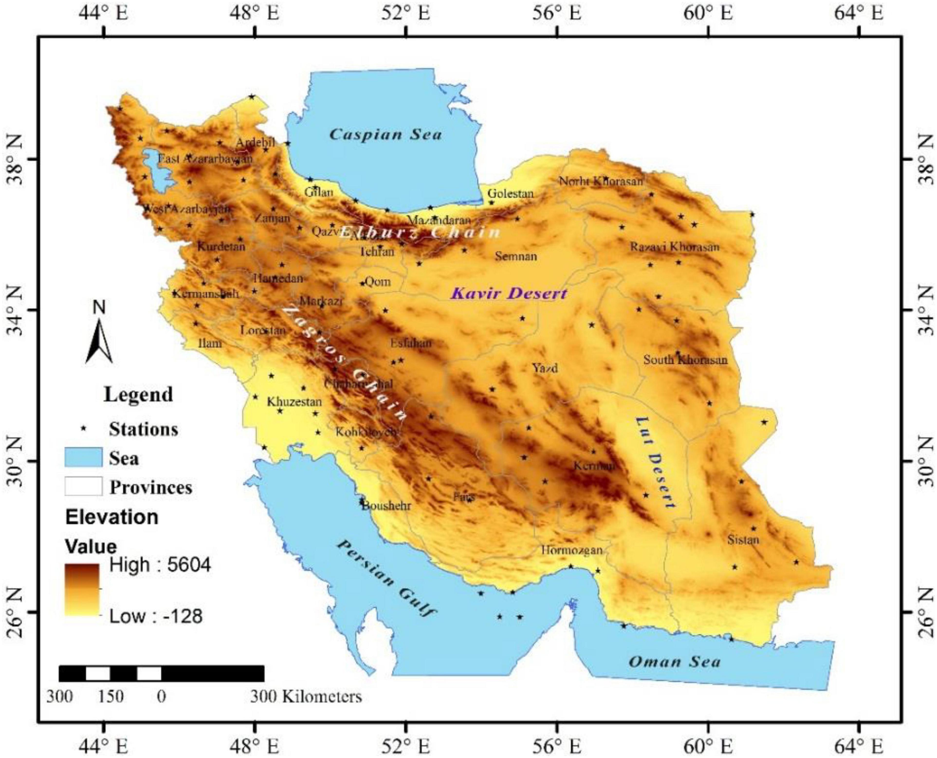
Figure 1. Topographical map of the study area and distribution of synoptic weather stations during the period 1987–2019.

Data and Method of Data Analysis

Climate Data Acquisition and Preprocessing

In climate studies, the required minimum number of years is 30. In this study, an attempt was made to use the latest available data. Therefore, considering the 33-year period of climate data, the maximum spatial coverage of the studied stations is also considered. To calculate the wood decay risk, the monthly mean temperature and precipitation were extracted from 100 Iranian meteorological stations between 1987 and 2019. The homogeneity of the climatic data was tested by Runs Test, and its normality was evaluated against the Kolmogorov–Smirnov test (Gharekhani and Ghahreman, 2010). For the present research, the climatic regions were classified by De Martonne (1926) method (Figure 2) as a common classification method within climatological studies based on the mean annual precipitation (mm) and temperature (^°C) of the regions. De Martonne’s climate zones are classified according to the aridity index (AI) values as follows (Croitoru et al., 2013):

FIGURE 2

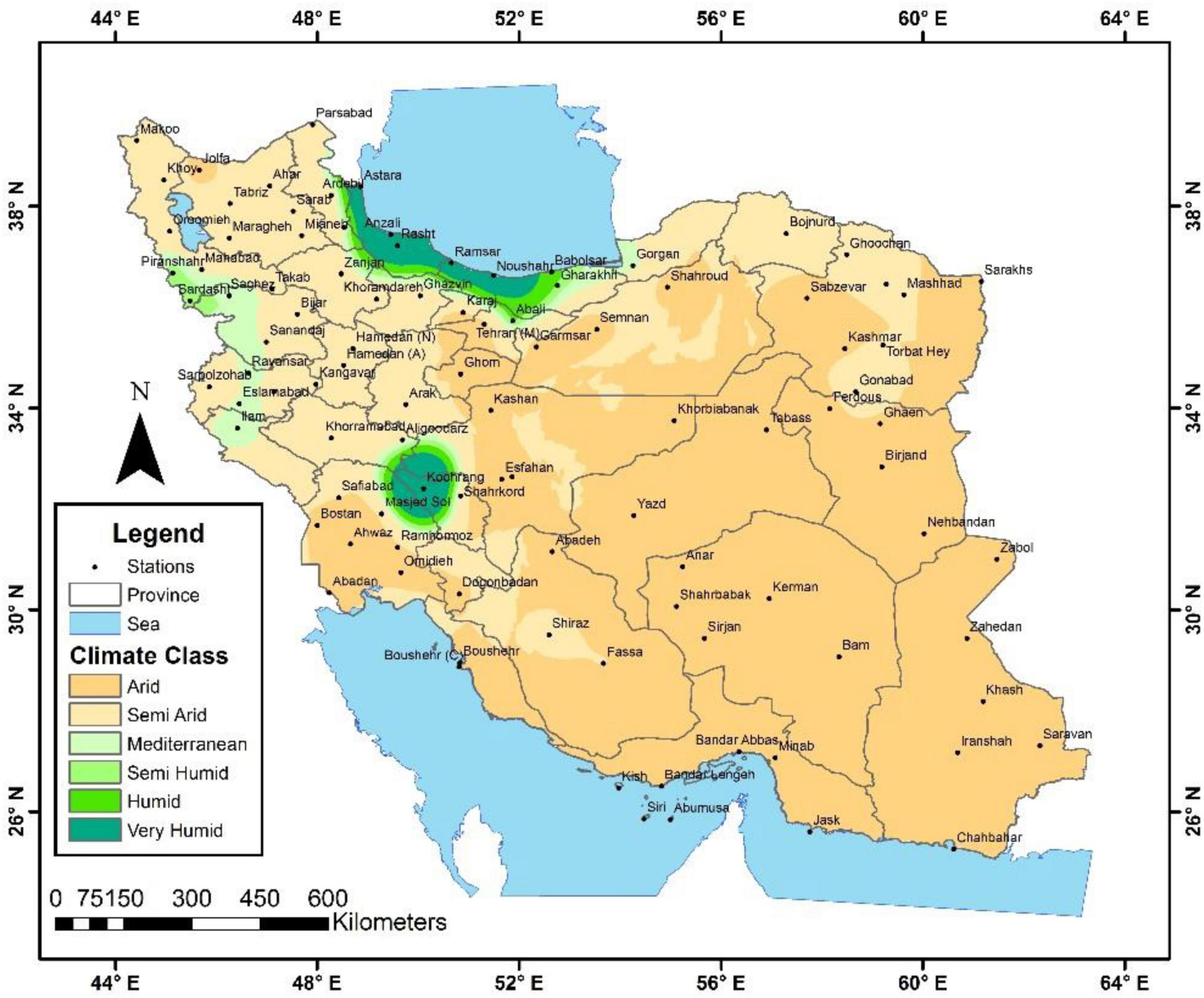
Figure 2. Geographical locations and climate zones of studied stations based on De Martonne (1926).

$$AI=P/\left(T+10\right)(1)$$

where P and T stand for the mean annual precipitation (mm) and mean annual temperature (^°C), respectively, and the value of AI categorizes the arid zone (AI < 10), semi-arid (10 ≤ AI < 20), Mediterranean (20.0 ≤ AI < 24.0), semi-humid (24.0 ≤ AI < 28.0), humid (28.0 ≤ AI < 35.0), very humid (35.0 ≤ AI ≤ 55.0), and extremely humid zones (AI > 55.0).

Scheffer Climate Index

The SCI is a popular index to characterize the site-specific relative hazard for above-ground wood decay, and it was determined by Eq. 2 according to Scheffer (1971) as follows:

$$SCI=\sum _{\text{Jan}}^{\text{Dec}}\left[\left(T-2\right)\left(D-3\right)\right]/16.7(2)$$

where T denotes the monthly average temperature (^°C) and D is the number of days with more than 0.25 mm of rainfall per month. The value ranges of SCI were determined and classified by Scheffer (1971) into three categories: low decay risk condition (less than 35), moderate decay risk (35–65), and high decay risk (more than 65). In this study, the SCI values zoning was performed using ArcGIS version 10.4.

Decadal and El Niño Southern Oscillation-Based Analysis of the Scheffer Climate Index

The ENSO time series datasets are available in https://ggweather.com/enso/oni.htm and plotted in Figure 3. According to Carll (2009), the year-to-year analysis of the SCI might differ from the periodic analysis, so in the first method, the decadal changes over the three periods of 1987–1997 (D1), 1998–2008 (D2), and 2009–2019 (D3) were averaged and their differences were analyzed in pairs (e.g., D1–D2, D1–D3, and D2–D3). Carll (2009) also argued that studies of wood decay risk should be based on patterns or climate teleconnection indices as well. Hence, the mean SCI in different phases of ENSO (EL, LN, and N) were calculated and pair-wise differences (EL-LN, EL-N, and LN-N) were analyzed. For example, Helali et al. (2021) showed that the occurrence of Last Spring Frost and Chilling in Iran in different phases and intensities of ENSO varies from the long-term average. In this study, the average values of wood decay risk based on SCI were calculated.

FIGURE 3

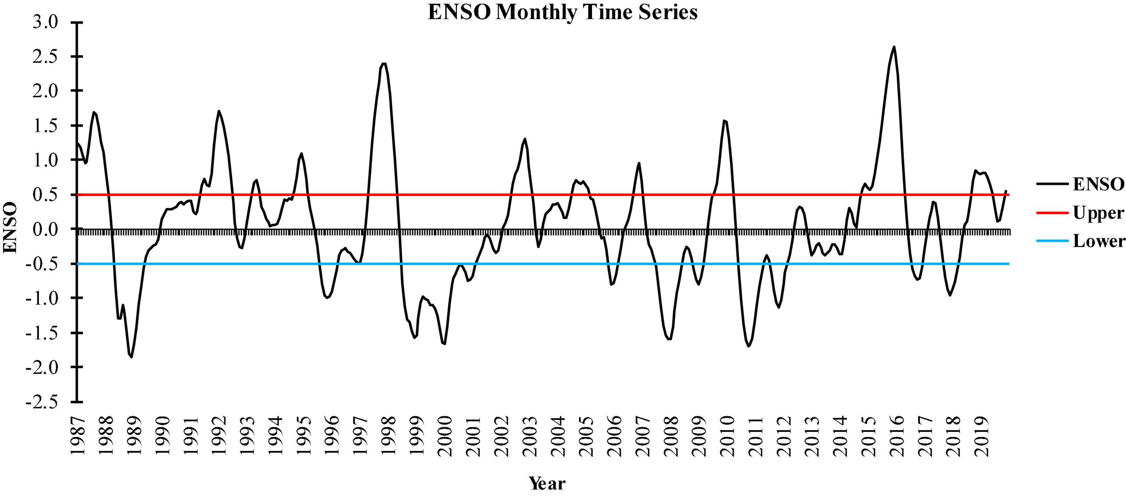
Figure 3. ENSO monthly time series (red and blue lines indicating El Niño and La Niña phases, respectively).

Trend Analysis

The changes of SCI values over time were analyzed using two different methods, the Mann–Kendall (Mann, 1945; Kendall, 1975) and Sen’s slope (Sen, 1968) test. The Mann-Kendall test is suggested by The World Meteorological Organization for trend analysis of climate variables (WMO, 2004). In time series, intensity of a variable at a time depends on its intensity in the past or in the future, and it is defined as autocorrelation. Autocorrelation increases the probability of significant trend in the time series (Partal and Kahya, 2006; Karmeshu, 2012); therefore, in this research, the autocorrelation effect was eliminated by the pre-whitening approach (von Storch and Navarra, 1999). Then, trend analysis was performed using a Mann–Kendall non-parametric test. This method is robust to outliers (Hirsch et al., 1993; Li et al., 2017) while missing data do not affect its performance. The null hypothesis of the Mann–Kendall test implies that the series are random without any trend, whereas the acceptance of the hypothesis is indicative of a trend in the time series data. First, the difference between each observation is calculated and it is applied by the mathematical sig function (sgn) to extract S parameter as follows (Ali and Abubaker, 2019):

$$S=\sum _{k=1}^{n-1}\sum _{j=k+1}^{n}sgn\left(x_j-x_k\right)(3)$$

$$sgn(\text{X})=\{\begin{array}{ccc}\hfill -1\hfill & \hfill \text{if}\hfill & \hfill X<0\hfill \\ \hfill 0\hfill & \hfill \text{if}\hfill & \hfill X=0\hfill \\ \hfill 1\hfill & \hfill \text{if}\hfill & \hfill X>0\hfill \end{array}(4)$$

where n defines the number of time series observations, and x_j and x_k are data from jth and kth time series, respectively. Second, the variance is calculated using Eq. (5):

$$\{\begin{array}{ccc}\text{Var}\left(S\right)=\frac{n-\left(n-1\right)\left(2n+5\right)-{\sum }_{i=1}^{m}t\left(t-1\right)\left(2t-5\right)}{18}\mathrm{\dots }\mathrm{\dots }..\hfill & \text{if}\mathrm{\dots }\mathrm{\dots }..\hfill & n>10\hfill \\ \text{Var}\left(S\right)=\frac{n-\left(n-1\right)\left(2n+5\right)}{18}\mathrm{\dots }\mathrm{\dots }\mathrm{\dots }\mathrm{\dots }\mathrm{\dots }\mathrm{\dots }\mathrm{\dots }\mathrm{\dots }\mathrm{\dots }\mathrm{\dots }..\hfill & \text{if}\mathrm{\dots }\mathrm{\dots }..\hfill & n<10\hfill \end{array}(5)$$

where n is the number of observational data, m is the number of series with redundant data, and t is the frequency of data with the same value. Finally, the Z statistic is obtained by one of the following expressions:

$$Z=\{\begin{array}{ccc}\frac{S-1}{\sqrt{\text{Var}\left(S\right)}}\mathrm{\dots }\mathrm{\dots }\mathrm{\dots }\mathrm{\dots }\mathrm{\dots }\mathrm{\dots }\mathrm{\dots }.\hfill & \text{if}\mathrm{\dots }\mathrm{\dots }..\hfill & S>0\hfill \\ 0\mathrm{\dots }\mathrm{\dots }\mathrm{\dots }\mathrm{\dots }\mathrm{\dots }\mathrm{\dots }\mathrm{\dots }\mathrm{\dots }\mathrm{\dots }\mathrm{\dots }..\hfill & \text{if}\mathrm{\dots }\mathrm{\dots }..\hfill & S=0\hfill \\ \frac{S+1}{\sqrt{\text{Var}\left(S\right)}}\mathrm{\dots }\mathrm{\dots }\mathrm{\dots }\mathrm{\dots }\mathrm{\dots }\mathrm{\dots }\mathrm{\dots }.\hfill & \text{if}\mathrm{\dots }\mathrm{\dots }..\hfill & S<0\hfill \end{array}(6)$$

In a two-dimensional test for time series analysis, the null hypothesis is accepted if the following condition is fulfilled:

$$\left|Z\right|\le Z_{\mathrm{\alpha }/2}(7)$$

where α denotes the significance level of the test and Z_α is the standard normal distribution statistic at the significance level α. If the Z statistic is positive, the time series’ trend is upward (a positive value larger than 1.96 means a significant increasing trend), and if it is negative (a negative value lower than -1.96 indicates a significant decreasing trend), the trend is downward (Li et al., 2017).

Sen’s slope estimator test was utilized to calculate the magnitude of the trend in the SCI time series. It is based on calculation of the median slope for time series to decide whether the slope is reliable at different significance levels or not. This type of test performs better than Mann–Kendall test in time series data with high frequency of duplicated data. To calculate this non-parametric statistical test, the slope between N pair of time series data was obtained by Eq. 8:

$$Q_{\text{med}}=\frac{X_j-X_i}{j-i}\mathit{\hspace{1em}\hspace{1em}\hspace{1em}\hspace{1em}\hspace{0.5em} }\text{for}\{\begin{array}{c}i=1\mathrm{\dots }N\hfill \\ j=\mathrm{\hspace{0.17em}1}\mathrm{\dots }N\hfill \end{array}(8)$$

where X_i and X_j represent values data at time j and i, respectively, and N is equal to the number of data pairs. It is calculated by Eq. 9 (n is number of time series data):

$$N\mathrm{`}=\frac{n\left(n-1\right)}{2}(9)$$

The series of slopes [median (Q_med)] are calculated according to even–odd number of N (Sen, 1968; Gocic and Trajkovic, 2013). In the present study, the median slope of the annual SCI was used to calculate the median slope for a 33-year period. In addition, the Mann–Kendall test significant (greater than +1.96 and less than -1.96) and non-significant (between +1.96 and -1.96) trend zoning was mapped by ArcGIS version 10.4.

Interrelationships Between Scheffer Climate Index With Climate Variables and El Niño Southern Oscillation

The Pearson correlation method was used to investigate the effect of climate variables (mean temperature and frequency of precipitation more than 0.25 mm) on the SCI as follows:

$$R=\frac{\sum \left(x-\overline{x}\right)\left(y-\overline{y}\right)}{\sqrt{{\left(x-\overline{x}\right)}^2{\left(y-\overline{y}\right)}^2}}(10)$$

where x and y represent climate and ENSO variables, y denotes SCI values, $\overline{x}$ is the mean of climate variables and ENSO (i.e., mean temperature, precipitation, and ENSO in 30 years), and $\overline{y}$is the mean of SCI values (i.e., mean SCI in 30 years), respectively. Consequently, the correlation coefficient between the SCI and climate variables (mean temperature and frequency of precipitation more than 0.25 mm) was analyzed along with the trend analysis of climate variables using both the Mann–Kendall method and Sen’s slope estimator method. Finally, an attempt was made to investigate the spectral coherent analysis between the SCI and ENSO at all climates of Iran. Spectral coherence measures the linearity between the amplitudes and phases of two variables (Biltoft and Pardyjak, 2009). It calculates the correlation coefficient of frequency dependence. The spectral coherence is calculated by Eq. 11:

$$\text{CH}\left(f\right)=\frac{{\left|A_{\text{SE}}\left(f\right)\right|}^2}{\left|S_{\text{SS}}\left(f\right)\right|\left|S_{\text{EE}}\left(f\right)\right|}(11)$$

where f denotes the frequency of dependent value and A_SE(f) is the value of cross spectrum. The autospectral density value for variable ENSO is defined by |S_EE(f)| and for variable SCI is determined by |S_SS(f)|. The spectral coherence value is calculated between zero and unity for each frequency meaning no correlation to perfect correlation, respectively.

Results and Discussion

Spatial Differences of Scheffer Climate Index in Iran

The mean SCI values are shown in Figure 4. None of the stations showed a high decay risk, but a limited number of stations, mainly those stations in the southern shores of the Caspian Sea, had a medium decay risk.

FIGURE 4

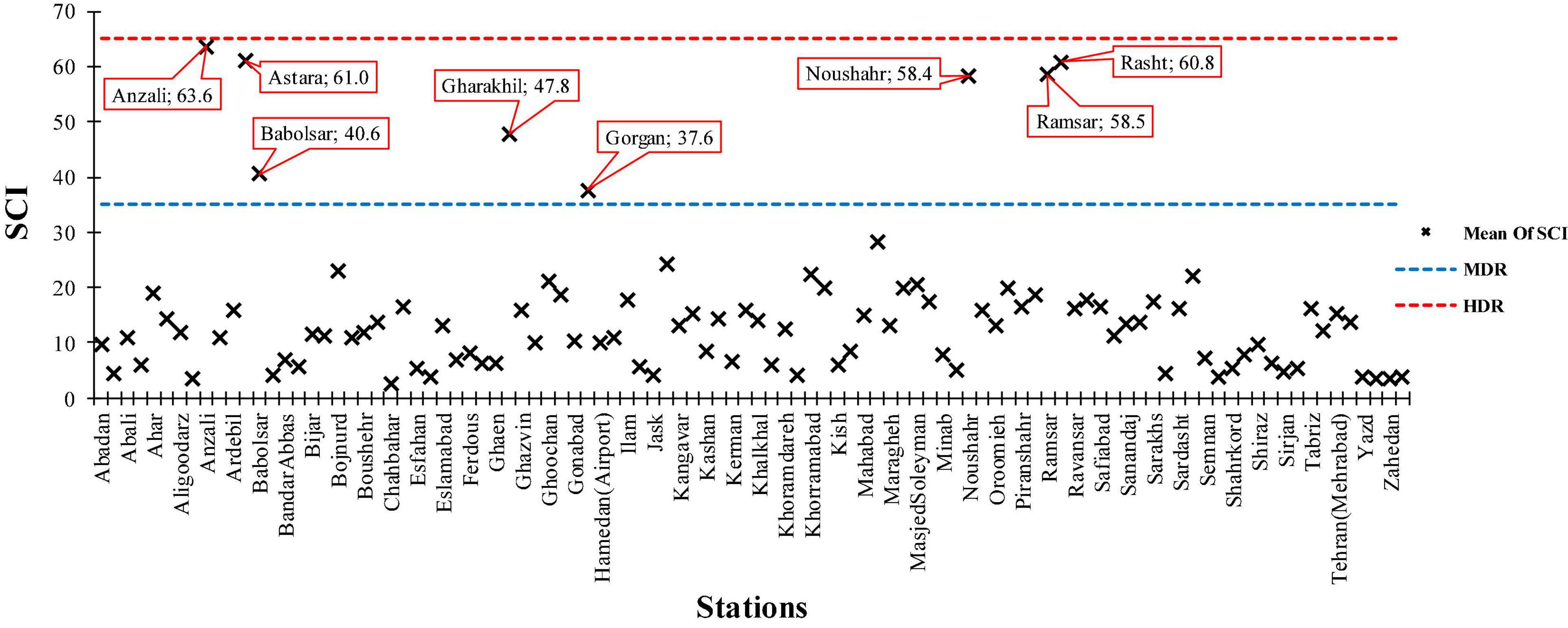
Figure 4. Mean values of SCI for studied stations during the period 1987–2019 (MDR and HDR: moderate and high decay risk base values, respectively).

The mean SCI values (Table 1) in Iran were mapped for the period 1987–2019 (Figure 5). The SCI varied between 2 and 75. The lowest SCI was determined for the south, the southeast, and the central plateau and for some regions in the west of Iran, as expressed through SCI contour lines of 5 and 10. Moreover, the SCI fluctuated between 15 and 25 in the southwest (major parts of Khuzestan, Lorestan, Kohgiloyeh, and Ilam), northwest (north and south parts of West Azarbayjan, East Azarbayjan, Ardebil, the northern parts of Tehran, Alborz, and Qazvin provinces), and northeast (some parts of East Golestan, Northern Khorasan, Northern Razavi Khorasan, and northeast of Semnan). Finally, the northern part of Iran (i.e., Anzali, Astara, Babolsar, Gharakhil, Gorgan, Noshahr, Ramsar, and Rasht) showed SCI values above 35 referring to a moderate decay hazard along the Caspian Sea coast (Table 1). Hence, the decay potential of wood products in most parts of Iran was low, except the north of Iran (Caspian Sea’s coastal areas) that was mostly at moderate risk and partially representing high decay risk.

TABLE 1

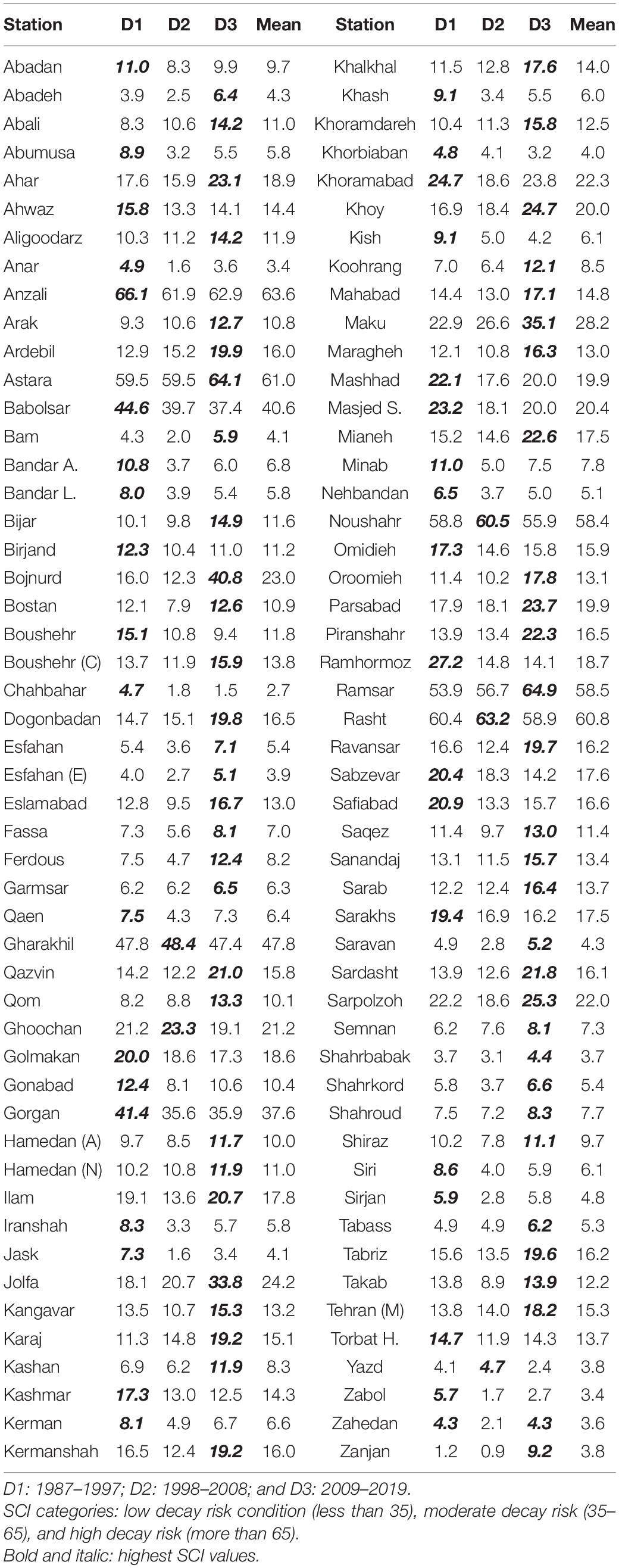
Table 1. The SCI during different decades between 1987 and 2019 at Iranian stations.

FIGURE 5

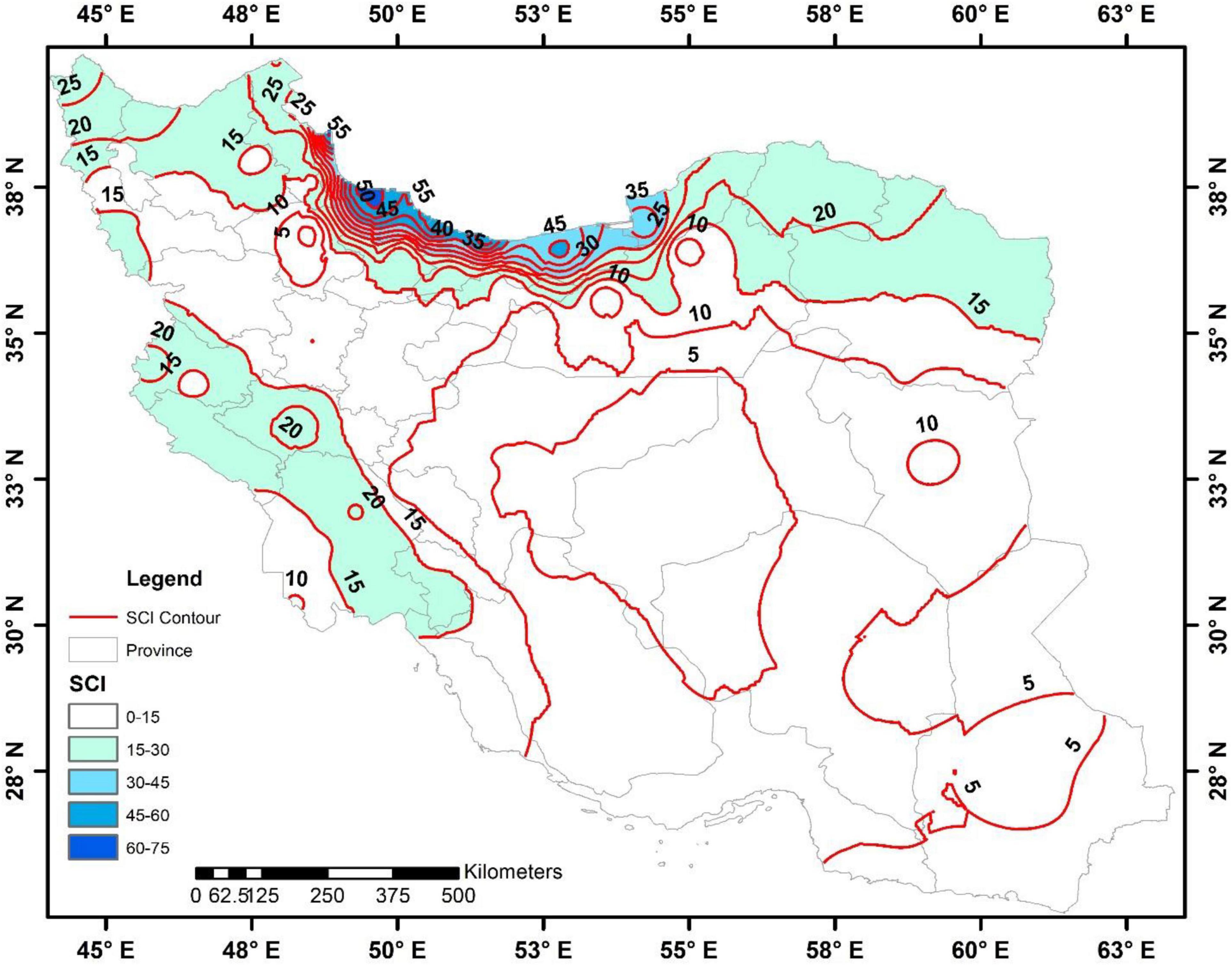
Figure 5. Mean SCI values in Iran during the period 1987–2019.

Decadal Scheffer Climate Index Changes

In this section, the SCI was analyzed during three decades (D1, D2, and D3, Figure 6, Table 1). Differences between decades are illustrated in Figure 6 and mapped in Figure 7. The highest mean SCI (the highest obtained values in each region) occurred in 37 stations of D1, 5 stations of D2, and 58 stations of D3. Consequently, the highest mean SCI value occurred more in the D3 period. On the other hand, the lowest mean SCI (the lowest obtained values in each region) in the D1, D2, and D3 included 16, 71, and 13% of the stations, respectively; therefore, the lowest mean SCI value was more persistent in D2 (Figure 8). The investigation of SCI in the stations under study (Table 1) unfolded that, in D1, there was high risk of wood decay only in Anzali and a moderate decay hazard was determined for Astara, Babolsar, Gharakhil, Gorgan, Noshahr, Ramsar, and Rasht, although at other stations a low hazard was estimated. Likewise, the decade D2 represented a similar pattern as D1; however, during D3, Bojnourd and Maku showed moderate decay hazard together with those stations in D1 and D2.

FIGURE 6

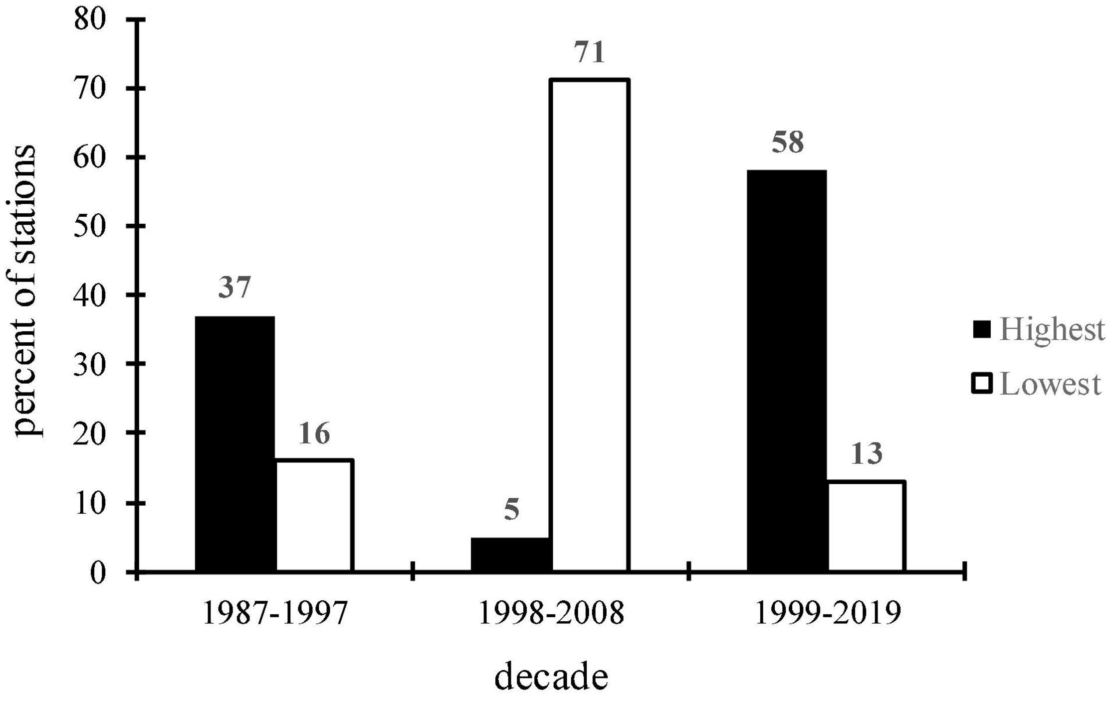
Figure 6. The percentage of stations with highest and lowest SCI value during different decades.

FIGURE 7

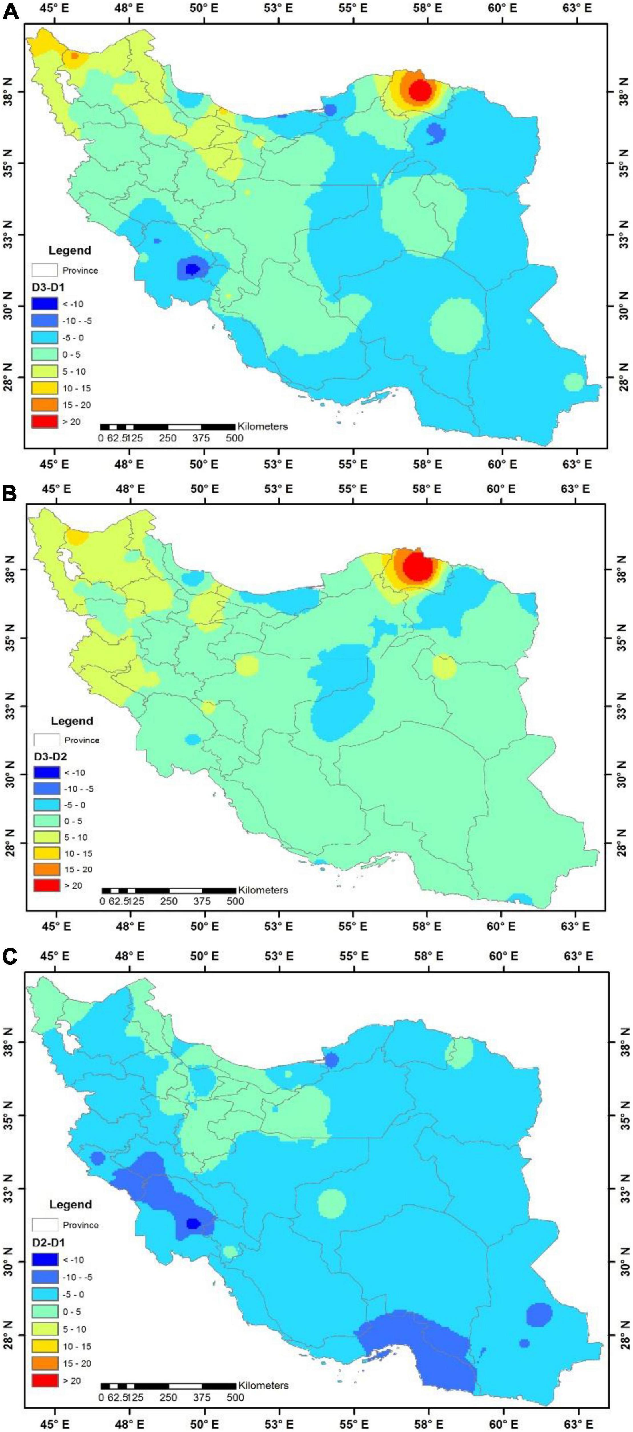
Figure 7. Differences of the SCI during three different decades: (A) D3–D1; (B) D3–D2; and (C) D2–D1.

FIGURE 8

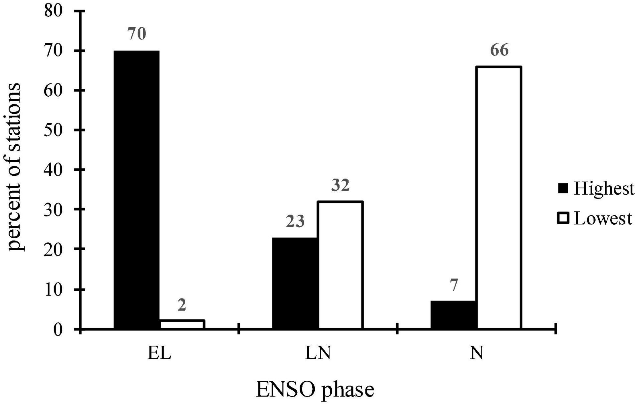
Figure 8. The percentage of stations with highest and lowest SCI value during different ENSO phases.

A comparison of the SCI values between the three decades (D1, D2, and D3) also showed that the SCI value in the D3 reduced by 5 compared with D1, mostly in the eastern and southeastern sections, the eastern part of the central plateau, the south, and southwest (Figure 7). Besides, a reduction of 10 was observed in small parts of Khuzestan and Razavi Khorasan, while an increase of 5 happened in the west part of the central plateau, east of Yazd, northwest of South Khorasan, Kerman Center, Hamedan, Ilam, Kermanshah, central Kurdestan, and south section of East and West Azarbayjan. Moreover, a decrease of 10 in SCI values was reported in Alborz, Qazvin, Zanjan, Ardabil, and north of West and East Azarbayjan provinces, and an increase of more than 15 occurred in small parts of North Azarbayjan and the whole of North Khorasan provinces. Making an analogy between D3 and D2, it was discovered that SCI values, in most parts of Iran, increased by 5 from D3 to D2 (also, by 10 in northwestern regions and more than 15 in North Khorasan), while in some parts of west of Yazd, east of Isfahan, western part of Razavi Khorasan, and the eastern part of Mazandaran, decreasing values of 5 were observed. Considering the changes from D2 to D1 period, mainly a decrease of 5 to 10 appeared in most of the regions (up to 10 in the southwest and southeast), but an increase of 5 appeared (Figure 7) in some parts of Tehran, west of Semnan, Markazi, Qazvin, Zanjan, Ardebil, and north of West and East Azarbayjan provinces. The diversity in the potential risk of wood decay demonstrated both decreasing and increasing in different decades depending on the various climate and geographical locations within Iran. In this case, various studies in Norway (Lisø et al., 2006), Europe with humid and warm regions (Viitanen et al., 2010), and North America (Morris and Wang, 2008; Carll, 2009) had been conducted and concluded that the variations in the potential risk of wood decay were predominantly increasing and had spatial variations as well.

Scheffer Climate Index Changes During Different El Niño Southern Oscillation Phases

The SCI was determined for three different ENSO phases including EL, LN, and N phases (Table 2 and Figure 8). In addition, SCI differences were evaluated in pairs and mapped in Figure 9. The results showed that the highest mean SCI predominantly occurred during EL phases, comprising 70% of the stations, while in LN and N phases, only 23 and 7% of the stations showed the highest SCI values, respectively, (Table 2). Therefore, most of the studied stations had the highest mean SCI in the EL phase. Aside from that, the lowest mean SCI mainly occurred in N phase (66% of the stations) followed by LN and EL phases, for 32 and 2% of the stations, respectively, (Table 2 and Figure 8). So, in N phase, most of the stations were dominated by the lowest mean SCI.

TABLE 2

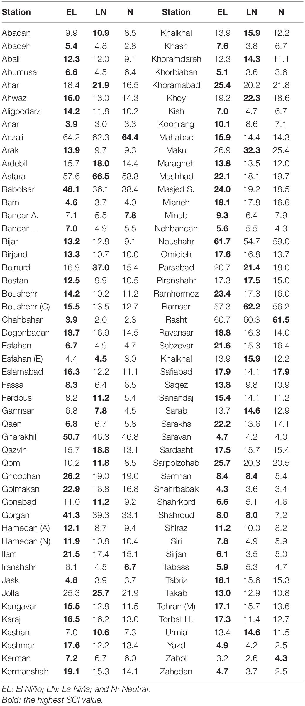
Table 2. SCI values during different ENSO phases.

FIGURE 9

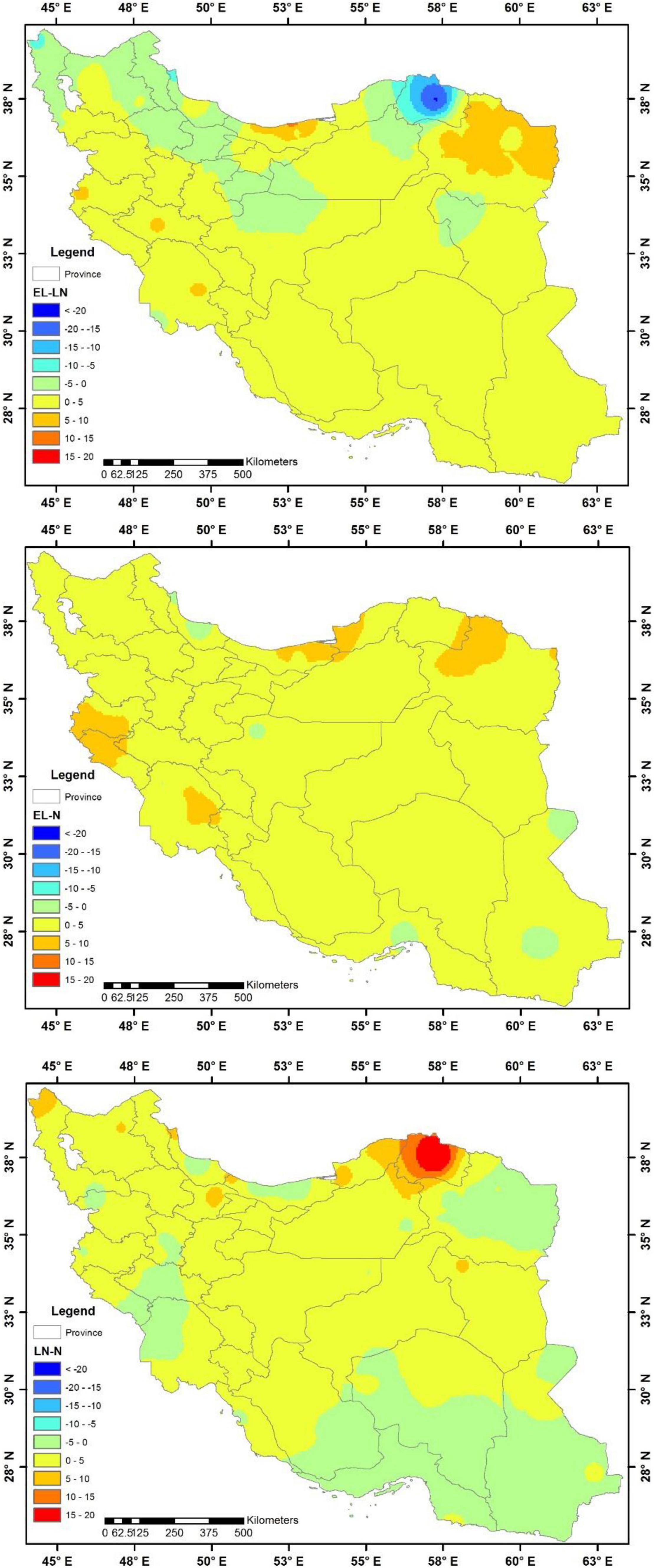
Figure 9. Differences of the SCI during different ENSO phases.

We compared the SCI during different ENSO phases (Figure 9). In detail, SCI values in EL compared with LN exhibited a growth of 5 (in major regions of the country) and 10 (in Mazandaran, Razavi Khorasan, Khuzestan, and Lorestan), while the SCI decreased up to 5 in some parts of Northern Isfahan, Qom, Markazi, Qazvin, Zangan, Ardebil, East and West Azarbayjan, northwest of South Khorasan, northeast of Semnan, and west of Golestan. The SCI value showed up to 10 points drop in parts of North Khorasan and small parts of West Azarbayjan. Comparison of the EL with N phase revealed the SCI value mostly increased by 5 in all regions, and up to 10 in some parts of North Khorasan, Mazandaran, Kermanshah, Ilam, and Khuzestan, while the SCI values decreasing up to 5 were observed in small sections of Sistan and Golestan. Therefore, the SCI changes from EL to N phase represented 5 to 10 increments. Changes in the SCI from LN to N phase showed an increase of 5 (in central plateau, eastern part, northwest, and west of Iran), 10 (in small parts of West Azarbayjan, Qazvin, Golestan, northeast of Semnan), and more than 15 in North Khorasan. Particularly, there was a decrease of 5 in the SCI in north and west of Khuzestan, central Lorestan, south of Ilam, central part of Gilan, Mazandaran, Razavi Khorasan, and south and southeast of Iran. Therefore, it can be concluded that the changes of SCI from LN to N phase, in different regions, had increasing or decreasing trend up to 15. As it was mentioned earlier in the Introduction, Morris and Wang (2008) emphasized those periodic patterns of teleconnection indices (e.g., PDO) could attribute to the wood decay index. In this study, it was found that changes in the SCI in different phases of ENSO followed a different pattern, so that the highest value of SCI was mainly observed in the El Niño and the lowest in the Neutral phase, and their differences varied in different regions and stations. ENSO influences the climate factors (Maryanaji et al., 2019) and might show a significant correlation with precipitation systems in some regions (Helali et al., 2020). The influence of the ENSO teleconnection patterns also highlighted that the wood decay risk values vary in different phases, with the highest SCI values in the El Niño (70% of the stations) and the lowest value in the Neutral phase (66% of the stations). Using ENSO in three phases and its anticipations also led to more accurate SCI fluctuation predictions in terms of temperature and precipitation. Therefore, precipitation increases and decreases in the El Niño and La Niña phases create a rise and decline in the risk of wood decay, respectively.

Trend Analysis of the Scheffer Climate Index

The trend analysis of the SCI revealed some decreasing or increasing changes in Iran, all over the region. Based on the analysis, the changes of SCI were insignificant in most parts of the country except in the northwest, west, and to some extent in the central regions. According to the results, a significant decreasing trend was only found for a small part of Khuzestan in the southwest of the country, whereas a significant increase of SCI was observed in the wide areas of Markazi, Tehran, Alborz, Qazvin, Zanjan, Ardebil, East and West Azarbayjan, Kurdestan, Kermanshah, and Ilam (Figure 10).

FIGURE 10

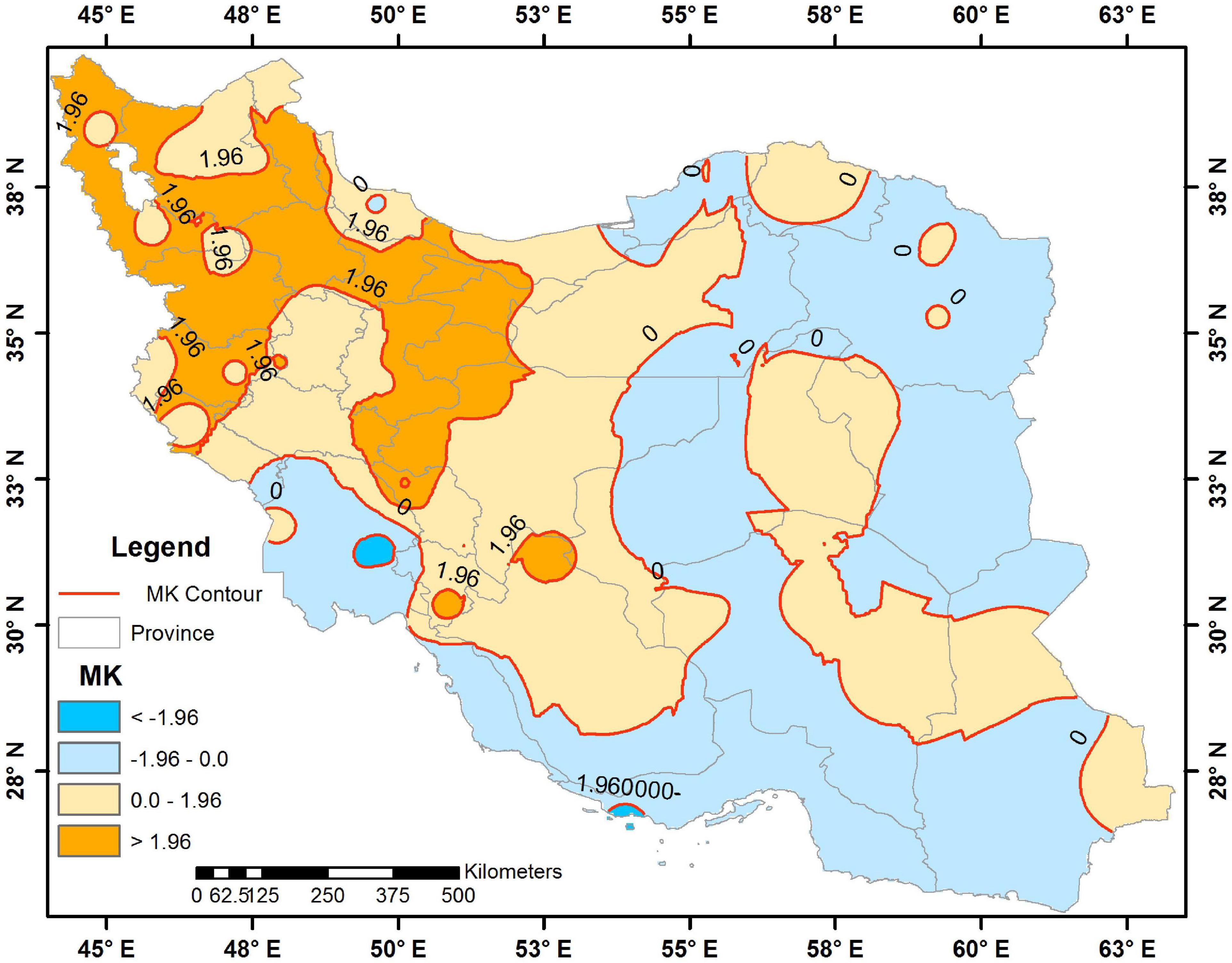
Figure 10. Mann–Kendall (MN) trends and significant (greater than +1.96 and less than −1.96) and non-significant (between +1.96 and −1.96) contours of the SCI in Iran.

Examination of the slope changes of the SCI over the 33-year period also remarked that it varied between -15 and 15 in the study area. The fluctuation rates were recorded between -5 and +5 in the south, central plateau, southwest, northeast, and small parts of Hamedan and Lorestan provinces (in most parts of northwest and west of Iran an increase of 5 up to 10 and a growth of 10 to 15 in the northern parts of Azarbayjan and Alborz). Furthermore, a drop was presented only in parts of Razavi Khorasan and Khuzestan that exceeded 10 (Figure 11). Trend analysis confirmed an increasing trend of SCI in 66% of the stations and a decrease in 34% of them, which was significant only in the northwest, west parts, and to some extent in the central regions, with the variation of -15 to 15 over the 33-year period. Carll (2009) and Morris and Wang (2008) found the increase in the mean SCI by 1.5 and 4.7, in Canada and the United States, respectively, during 30 years (1971–2000). In our study across Iran, the average of 2.9 for SCI with an increasing trend was recorded during 33 years.

FIGURE 11

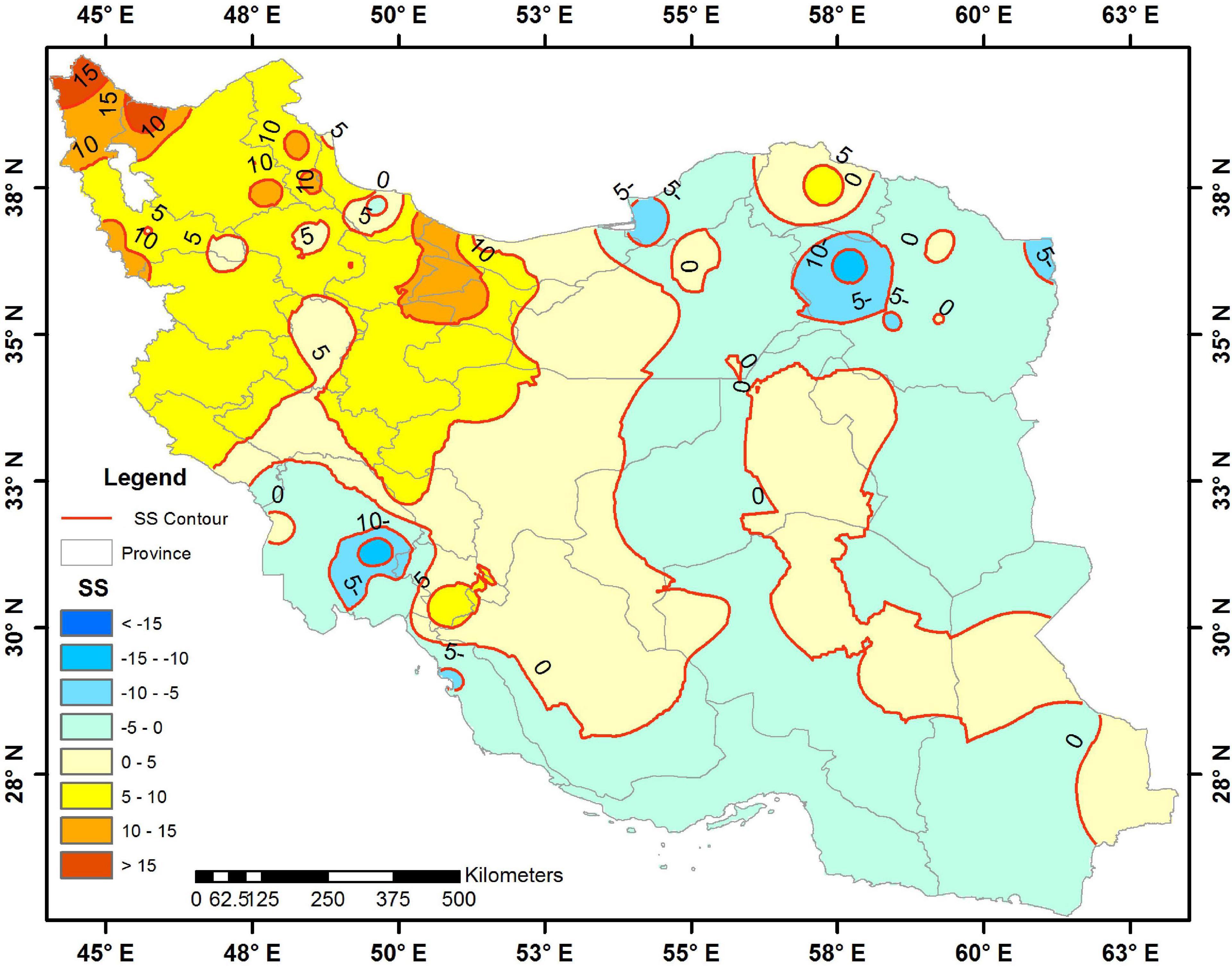
Figure 11. Sen’s slope (SS) contours of the SCI in Iran.

The Causative Factors of the Scheffer Climate Index Trend

Since the SCI is subjective to the temperature and amount and distribution of precipitation, it is needed to investigate the relationship between those causative factors and the SCI. Therefore, the trend of changes in temperature, precipitation, and the SCI were explored and correlations of SCI with temperature and precipitation were analyzed according to the climatic zones (Table 3).

TABLE 3

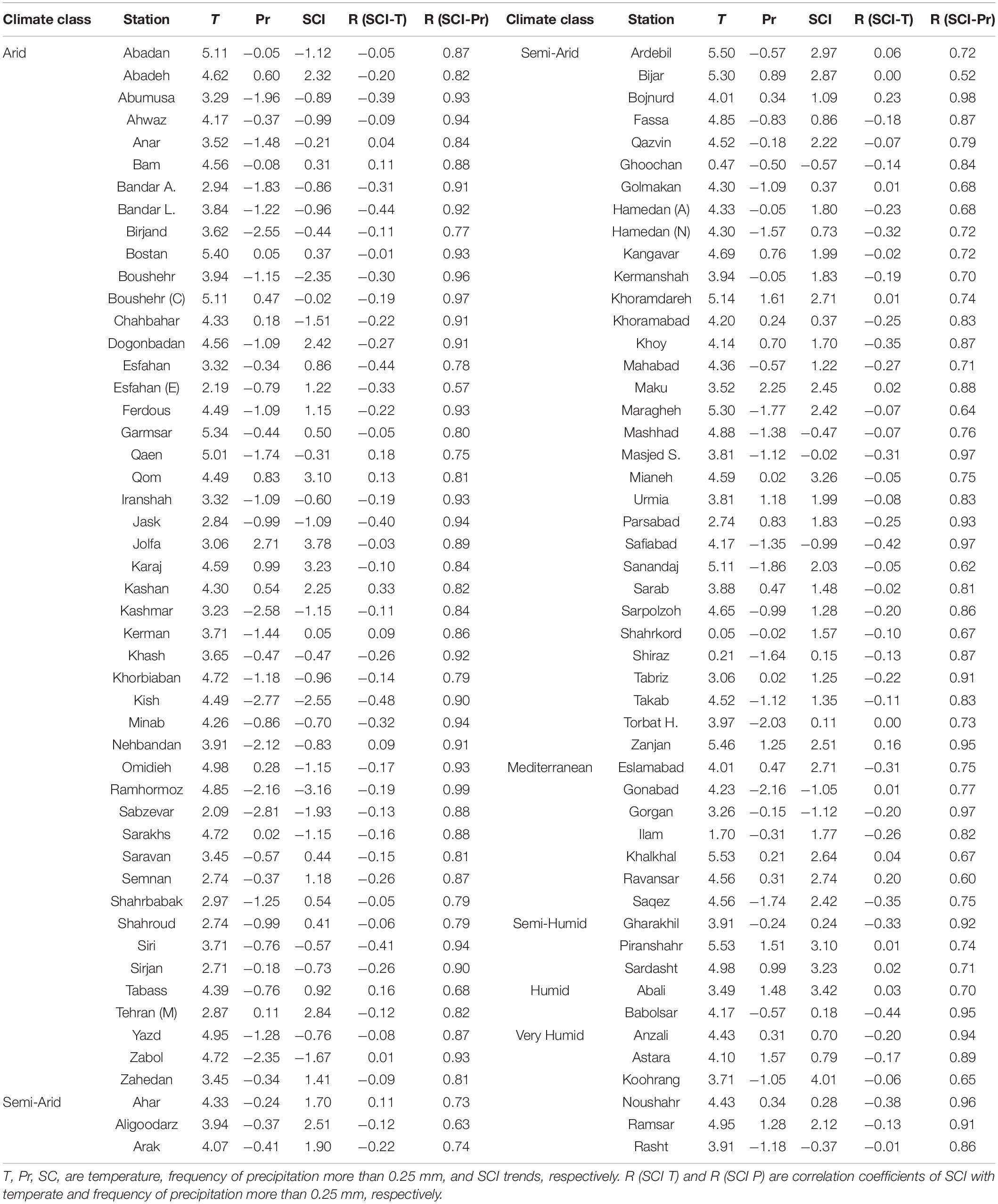
Table 3. Temperature, precipitation, and SCI trends and SCI Pearson correlation with temperature and precipitation frequency above 0.25 mm.

In arid climates (represented by 47 stations), the mean temperature trend was mainly upward, while precipitation was increasing (significant in Jolfa) and decreasing (significant in Abumusa, Birjand, Kashmar, Kish, Nahabandan, Sabzevar, and Zabul). Also, the trend of SCI was positively increased in the 20 stations (but significant in Abadeh, Doganbadan, Qom, Jolfa, Karaj, Kashan, and Tehran) and negative in 3 stations (but significant in Bushehr, Kish, and Ramhormoz). Based on the trend analysis results, increasing temperature and decreasing number of rainy days caused an increase in SCI. The correlation coefficient values of the SCI regarding precipitation and temperature varied from 0.57 to 0.99 and −0.48 to 0.33, respectively.

In semi-arid climates (i.e., 35 stations), the trend of temperature was increasing and significant as well in all 35 stations, whereas precipitation at 31 stations had a decreasing trend (significant at Torbat H.) and 14 stations marked increasing trend (significant at Maku). Consequently, the trend of SCI at 31 stations were positive (significant in Aligoodarz, Ardebil, Bijar, Qazvin, Kangavar, Khoramdareh, Maku, Maragheh, Mianeh, Urmia, Sanandaj, and Zanjan) and at 4 stations were decreasing (non-significant). Due to increasing trend of temperature and increasing trend of precipitation, an increasing trend of SCI happened in Ahar, Ardebil, Bojnurd, Fassa, Khoramdareh, Khoy, Maku, Mianeh, Urmia, Parsabad, Sarab, Shiraz, Tabriz, and Zanjan. In contrast, decreasing trend of precipitation caused a decreasing trend of SCI in Aligoodarz, Arak, Bijar, Qazvin, Quchan, Golmakan, Hamedan (N), Hamedan (A), Kangavar, Kermanshah, Khoramabad, Mahabad, Maragheh, Mashhad, Safiabad, Sanandaj, Sarpol Zahab, Shahrekord, Takab, and Torbat H. The outcomes showed that the values of correlation coefficient of SCI varied from 0.52 to 0.98 (with precipitation) and from -0.42 to 0.23 (with temperature) with 27 stations in negative and 8 stations in positive values.

In terms of the Mediterranean climate, which was presented in seven stations, the temperature trend increased significantly at all seven stations, while the precipitation trend decreased at five stations (significant in Gonabad) and two other stations had an increasing trend, and thus, the trend of SCI showed a significant increase (without a decreasing trend) at four stations (i.e., Eslamabad, Khalkhal, Ravansar, and Saqez stations). Also, the correlation coefficient values for the SCI with precipitation and temperature ranged from 0.6 to 0.9 and -0.35 to 0.2, respectively. Due to the increasing trend of temperature in all stations, it was observed that the increasing trend of precipitation resulted in an increasing trend of SCI in both Eslamabad and Khalkhal stations. In contrast, in Gonabad, Gorgan, Ravansar, and Saqez stations, a decreasing trend of precipitation led to an increasing trend of SCI. As a consequence, it might be concluded that the trend of SCI has been more influenced by temperature or amount of precipitation than frequency of precipitation greater than 0.25 mm.

The results demonstrated that in semi-humid climates including three stations (Piranshahr, Sardasht, and Gharakhil), all three stations experienced a significant increase in temperature and non-significant precipitation, which caused an increase in the trend of SCI at two stations (Piranshahr and Sardasht). Studies showed that the SCI experienced an increasing trend with increasing temperature and precipitation trend. The correlation coefficient values of SCI with precipitation and temperature were from 0.71 to 0.97 and -0.33 to 0.02, respectively. Therefore, there was no perfect correlation between the SCI and temperature, whereas it was highly correlated with precipitation frequency greater than 0.25 mm. Thus, in the semi-humid climate, the effect of increasing temperature and precipitation, simultaneously, led to an increasing trend of SCI.

The results of trend analysis and correlation coefficient in humid climate suggested that the temperature trend in both stations was increasing, but the precipitation trend in Abali station was increasing and Babolsar was decreasing, which can be attributed by the different topographic and geographical characteristics of the two stations (due to Abali’s height and Babolsar’s adjacency to coastal area). However, the trend of the SCI for both stations was increasing. The correlation coefficient values of SCI with precipitation and temperature varied from 0.70 to 0.96 and 0.03 to 0.44, respectively.

Based on the results in the humid climates of Iran, there was an increasing trend of SCI due to the influence of precipitation, temperature, as well as geographical and topographical characteristics. In very humid climates mainly located in the southern part of the Caspian Sea and coastlines (except for Koohrang), the trend of increasing temperature was significant and precipitation was mainly increasing and non-significant. Therefore, it caused an increasing trend of SCI. In this case, although the increasing trend of precipitation was non-significant, the increasing temperature caused an increase of wood decay risk. The result showed that the correlation of SCI with precipitation and temperature, in very humid climates, ranged between 0.65 to 0.96 and -0.01 to -0.38, respectively. According to our findings, the climate variables that caused the changes in SCI and the precipitation index had a greater impact on this trend, although the study by Lisø et al. (2006) highlighted the temperature rise as the only causative factor for the increase in the SCI.

Correlation of Scheffer Climate Index and El Niño Southern Oscillation

The Pearson correlation between SCI and ENSO is shown in Figure 12. The results revealed that the monthly ENSO was positively correlated with SCI at most of the stations, and minimally there was a negative correlation between them at stations. The significant positive correlation is mainly concentrated in the northeastern, northern, southwestern, and western parts, while no significant negative correlation was observed. Previous studies (Nazemosadat and Cordery, 2000; Helali et al., 2020) showed that rainfall in Iran was correlated with the ENSO phenomenon, where rainfall was above the average during El Niño phases and below the average during La Niña phases. Thus, the ENSO phenomenon is also affecting the decay risk of wood, which is consistent with the findings from this study.

FIGURE 12

Figure 12. The correlation of SCI and ENSO during different months.

Spectral Coherence Analysis of Scheffer Climate Index and El Niño Southern Oscillation

Due to the large number of stations, spectral coherent analysis was performed on the climate classes (i.e., Arid, Semi-Arid, Mediterranean, Semi Humid, and Very Humid), and their results are presented in Figure 13. According to the results, it is clear that in most of the studied climates, the maximum values of SCI do not correspond to the maximum values of ENSO and are associated with lag time. Therefore, the interpretation of SCI extreme values is not justifiable by only relying on the ENSO values. Since large-scale teleconnection indices (such as ENSO) indirectly affect the climate variables and SCI values, they associate with greater uncertainty. To reduce this uncertainty, the relationship between the SCI and large-scale teleconnection indices and other climatic variables can be analyzed. In studies of station correlation with large-scale teleconnection indices, due to the mismatch of spatial scale between two phenomena, different correlations are observed in surrounding areas; however, microclimatic effects are considered instead (Ghasemi and Khalili, 2008). In the spatial studies, the effect of teleconnection indices (e.g., ENSO) in the whole region or climatic zones was not fully studied yet, and the effect of microclimates and local zones is usually ignored (Helali et al., 2020). Therefore, to investigate the relationship between large-scale teleconnection indices and climatic variables (and SCI), the effect of spatial distribution of meteorological stations and homogeneity and completeness of datasets must be considered. Based on the spectral coherent analysis, the relation between SCI and ENSO in different climates of Iran was not considerable. However, using Pearson analysis showed significant correlations between SCI and ENSO in some parts of the study area. Therefore, the SCI extreme values and their correlations with ENSO indices might not be reliably interpreted by the spectral coherent analysis.

FIGURE 13

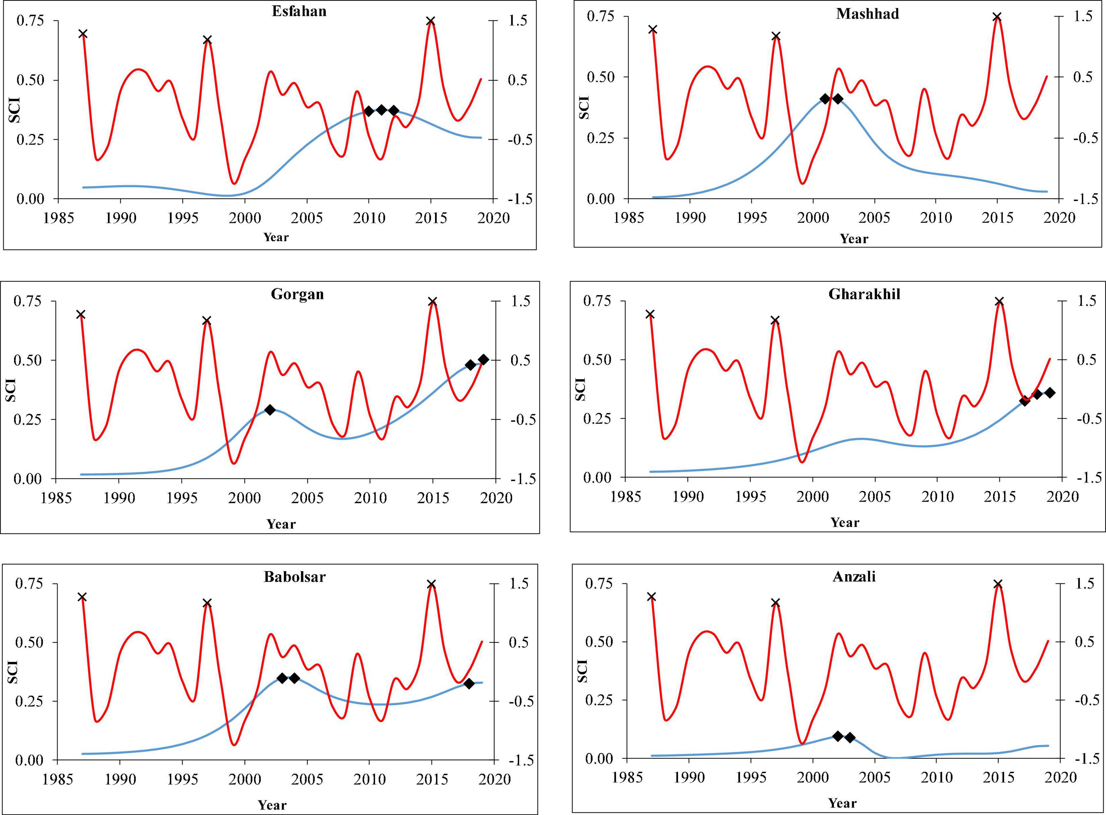
Figure 13. Spectral coherence values of SCI and ENSO in different climates of Iran (Esfahan: Arid; Mashhad: Semi-Arid; Gorgan: Mediterranean; Gharakhil: Semi Humid; Babolsar: Humid; and Anzali: Very Humid).

Our findings showed that predominantly Iran has a low potential for wood decay risk, and this study can be used to define the standard and criteria for deploying wooden material in the construction. In addition, climate change and its oscillation will affect wood quality and wood decay rate. The results also proved that some parts of the country (e.g., north, northwest, west, and northeast) might be more vulnerable to the wood decay risk as a result of climate variable changes during the last 33 years. Therefore, the wood-based construction materials should be cautiously deployed in those parts, and the buildings must be frequently observed based on the decay model in the region. The high-risk wood decay in coastal areas in the north of Iran suggests replacing wooden materials or prolonging wood service life and durability by extra preservative treatments. Consequently, the main parts of Iran had a low-risk potential of wood decay, which can be considered a strategy for revising the use of steel and concrete structures that should be addressed, evaluated, and compared with wood in terms of cost-effectiveness and environmentally friendly materials in future studies. Bayatkashkoli et al. (2008) reported the wood import industry in Iran by 200 million dollars. Bayatkashkoli (2011) outlined that the import rate of wooden products has been intensively increased. Moreover, Mollahassani et al. (2013) showed a 17.1% increase in wood import in a 10-year period (2000–2010) that directly affects the gross domestic product. Then, the results of this study could be used for appropriate decision-making to manage the exploitation of domestic wood production and resources and decrease massive wood imports for the supply market.

Conclusion

Wood decay risk is a quantitative measurement affected by various factors and climate variables. Therefore, we aimed to estimate wood decay risk, as well as its changes and its relationship with climate parameters and ENSO’s different phases, in Iran. The results indicated that the mean SCI values fluctuated between 2 and 75 in the entire region of Iran, specifically in the south, southeast, central plateau, and to some extent in the west part (5 to 10), southwest, northwest and northeast (15 to 25), and south coast of the Caspian Sea (more than 35 and 75). The study area was categorized as low decay hazard area, except the small part of Iran adjacent to the Caspian Sea’s coastal areas with moderate and high risk. Decadal SCI analysis showed that the highest SCI values were in the third decade (2009–2019) and the lowest values were in the second decade. Studying of increasing/decreasing trend in the SCI and their triggering factors noted that all stations experienced significant and upward trend in temperature, in different climates of Iran. Meanwhile, the precipitation frequency more than 0.25 mm showed increasing or decreasing trend (according to different stations) and resulted in a significant trend in SCI in some regions. The correlation of SCI with precipitation was more than its correlation with temperature; thus, we could conclude that precipitation had more influence on the changes of SCI than temperature. Therefore, not only mean temperature variables and the frequency of precipitation more than 0.25 mm are accounted for the changes in SCI values but also the temperature limit indicators, relative humidity, equilibrium MC, and the amount of precipitation (both on an annual and monthly basis) must be investigated on the changes of wood decay index. The results of this study indicated that Iran’s climatic and spatial diversity caused various fluctuations in the mean SCI with an average increase of 2.9. It seems that modeling the wood decay risk needs more investigation based on other geographical variables (e.g., altitude) with considering the microclimate region as well as predominant climatic variables (temperature, humidity, and wood response parameters such as equilibrium MC), and it might provide a better insight into the potential wood decay risk, analysis, and its distribution. The result showed that the correlation between SCI and ENSO was mainly positive and in some cases significant. Therefore, increasing and decreasing precipitation in the El Niño and La Niña phases led to an increase and decrease of the wood decay risk, respectively. Due to the impact of climate factors on wood decay along with decadal climate change trends, future studies will be conducted on climate changes, other wood decay indices, and SCI changes based on various climate factors with focus on different topography in the region. From the construction point of view, it would create an extensive research opportunity for wooden structures in the future studies and plans. The prediction of wood decay and its trend based on climatic point of view will be beneficial to determine the durability and persistence of wooden materials in such region and climate. Hence, according to our investigation, the SCI values and expectance of wood decay will be anticipated according to climate phenomena such as ENSO. However, to analyze SCI values, not only ENSO should be considered but also the effect of other large-scale teleconnection indices. Not only the climate change is a threat to wood products but also insect attack and fungi should be considered when recommending wood as a substitute for steel and concrete structures. Therefore, future work will investigate the effect of meteorological factors, condensation, and fungal species using dose-response function in wood decay risk.

Data Availability Statement

The raw data supporting the conclusions of this article will be made available by the authors, without undue reservation.

Author Contributions

JH, HM, and ML acquired the data and conceptualized and performed the analysis. JH, HM, and VS wrote the manuscript, inspected and discussed the data, and results. CB refined the research plan and supervised the group. JH, VS, CB, and GE provided technical and professional insight, edited, restructured, and optimized the manuscript. All authors have read and agreed to the published version of the manuscript.

Conflict of Interest

VS was employed by the company Darya Tarsim Consulting Engineers Co. Ltd.

The remaining authors declare that the research was conducted in the absence of any commercial or financial relationships that could be construed as a potential conflict of interest.

Publisher’s Note

All claims expressed in this article are solely those of the authors and do not necessarily represent those of their affiliated organizations, or those of the publisher, the editors and the reviewers. Any product that may be evaluated in this article, or claim that may be made by its manufacturer, is not guaranteed or endorsed by the publisher.

Acknowledgments

The authors wish to sincerely thank and appreciate the Islamic Republic of Iran Meteorological Organization (IRIMO) for providing the data to perform the present study. Also, the authors would like to express their sincere gratitude to anonymous referee 1 for his/her useful comments and Alireza Karbalaei for performing spectral analysis to complete this research.

Supplementary Material

The Supplementary Material for this article can be found online at: https://www.frontiersin.org/articles/10.3389/ffgc.2021.693833/full#supplementary-material

References

Ahmadi, M., Salimi, S., Hosseini, S. A., Poorantiyosh, P., and Bayat, A. (2019). Iran’s precipitation analysis using synoptic modeling of major teleconnection forces (MTF). Dyn. Atmos. Oceans 85, 41–56. doi: 10.1016/j.dynatmoce.2018.12.001

CrossRef Full Text | Google Scholar

Ali, R. O., and Abubaker, S. R. (2019). Trend analysis using mann-kendall, sen’s slope estimator test and innovative trend analysis method in Yangtze river basin, China. Int. J. Eng. Technol. 8, 110–119.

Google Scholar

Almås, A. J., Lisø, K. R., Hygen, H. O., Øyen, C. F., and Thue, J. V. (2011). An approach to impact assessments of buildings in a changing climate. Build. Res. Inf. 39, 227–238. doi: 10.1080/09613218.2011.562025

CrossRef Full Text | Google Scholar

Asakereh, H. (2017). Trends in monthly precipitation over the northwest of Iran (NWI). Theor. Appl. Climatol. 130, 443–451. doi: 10.1007/s00704-016-1893-8

CrossRef Full Text | Google Scholar

Asakereh, H. (2020). Decadal variation in precipitation regime in northwest of Iran. Theor. Appl. Climatol. 139, 461–471. doi: 10.1007/s00704-019-02984-9

CrossRef Full Text | Google Scholar

Ascoli, D., Vacchiano, G., Turco, M., Conedera, M., Drobyshev, I., Maringer, J., et al. (2017). Inter-annual and decadal changes in teleconnections drive continental-scale synchronization of tree reproduction. Nat. Commun. 8:2205. doi: 10.1038/s41467-017-02348-9

PubMed Abstract | CrossRef Full Text | Google Scholar

Bayatkashkoli, A., Rafeghi, A., Azizi, M., Ameri, S., and Kabourani, A. (2008). Estimate of timber and wood products export and import trend in Iran. J. Agric. Nat. Resour. 15, 73–83.

Google Scholar

Bayatkashkoli, A. (2011). Studying imports of wood, paper and their products in the world and Iran from 1998 to 2007. Iran. J. Wood Pap. Ind. 2, 37–54.

Google Scholar

Beesley, J., Creffield, J. W., and Saunders, I. W. (1983). An Australian test for decay in painted timbers exposed to the weather. For. Prod. J. 33, 57–63.

Google Scholar

Biltoft, C. A., and Pardyjak, E. R. (2009). Spectral coherence and the statistical significance of turbulent flux computations. J. Atmos. Ocean. Technol. 26, 403–410. doi: 10.1175/2008JTECHA1141.1

CrossRef Full Text | Google Scholar

Boer, R., and Surmaini, E. (2020). Economic benefits of ENSO information in crop management decisions: case study of rice farming in West Java, Indonesia. Theor. Appl. Climatol. 139, 1435–1446. doi: 10.1007/s00704-019-03055-9

CrossRef Full Text | Google Scholar

Brischke, C., and Rapp, A. O. (2008). Dose–response relationships between wood moisture content, wood temperature and fungal decay determined for 23 European field test sites. Wood Sci. Technol. 42, 507–518. doi: 10.1007/s00226-008-0191-8

CrossRef Full Text | Google Scholar

Brischke, C., and Selter, V. (2020). Mapping the decay hazard of wooden structures in topographically divergent regions. Forests 11:510. doi: 10.3390/f11050510

CrossRef Full Text | Google Scholar

Brischke, C., and Thelandersson, S. (2014). Modelling the outdoor performance of wood products-a review on existing approaches. Constr. Build. Mater. 66, 384–397. doi: 10.1016/j.conbuildmat.2014.05.087

CrossRef Full Text | Google Scholar

Brischke, C., Welzbacher, C. R., Meyer, L., Bornemann, T., Larsson-Brelid, P., and Pilgård, A. (2011). Service Life Prediction of Wooden Components-Part 3: Approaching a Comprehensive Test Methodology. IRG/WP/11-20464. Stockholm: The International Research Group on Wood Protection.

Google Scholar

Byrne, M. P., and O’Gorman, P. A. (2018). Trends in continental temperature and humidity directly linked to ocean warming. Proc. Natl. Acad. Sci. U.S.A. 115, 4863–4868. doi: 10.1073/pnas.1722312115

PubMed Abstract | CrossRef Full Text | Google Scholar

Carll, C. G. (2009). Decay Hazard (Scheffer) Index Values Calculated from 1971–2000 Climate Normal Data. General Technical Report FPL-GTR-179). Madison, WI: United States Department of Agriculture, Forest Service, Forest Products Laboratory.

Google Scholar

Croitoru, A. E., Piticar, A., Imbroane, A. M., and Burada, D. C. (2013). Spatiotemporal distribution of aridity indices based on temperature and precipitation in the extra-Carpathian regions of Romania. Theor. Appl. Climatol. 112, 597–607. doi: 10.1007/s00704-012-0755-2

CrossRef Full Text | Google Scholar

De Martonne, E. (1926). Une nouvelle fonction climatologique: l’indice d’aridité. Meteorologie 2, 449–458.

Google Scholar

Fernandez-Golfin, J., Larrumbide, E., Ruano, A., Galvan, J., and Conde, M. (2016). Wood decay hazard in Spain using the Scheffer index: proposal for an improvement. Eur. J. Wood Prod. 74, 591–599. doi: 10.1007/s00107-016-1036-z

CrossRef Full Text | Google Scholar

Frühwald, E., Brischke, C., Meyer, L., Isaksson, T., Thelandersson, S., and Kavurmaci, D. (2012). “Durability of timber outdoor structures – modelling performance and climate impacts,” in Proceedings of the WCTE World Conference on Timber Engineering 2012, ed. P. Quenneville (Auckland: Engineering Challenges and Solutions), 295–303.

Google Scholar

Ghaedamini, H., Nazem, S. M. J., Kouhizadeh, M., and Sabziparvar, A. A. (2014). Individual and coupled effects of the ENSO and PDO on autumn dry and wet periods in the southern parts of Iran. Iran. J. Geophys. 8, 92–109. (In Persian)

Google Scholar

Gharekhani, A., and Ghahreman, N. (2010). Seasonal and annual trend of relative humidity and dew point temperature in several climatic regions of Iran. J. Water Soil Agric. Sci. Technol. 24, 636–646. (In Persian)

Google Scholar

Ghasemi, A. R., and Khalili, D. (2008). The association between regional and global atmospheric patterns and winter precipitation in Iran. Atmos. Res. 88, 116–133. doi: 10.1016/j.atmosres.2007.10.009

CrossRef Full Text | Google Scholar

Gocic, M., and Trajkovic, S. (2013). Analysis of changes in meteorological variables using Mann-Kendall and Sen’s slope estimator statistical tests in Serbia. Glob. Planet. Change 100, 172–182. doi: 10.1016/j.gloplacha.2012.10.014

CrossRef Full Text | Google Scholar

Helali, J., Momenzadeh, H., Asadi Oskouei, E., Lotfi, M., and And Hosseini, S. A. (2021). Trend and ENSO-based analysis of last spring frost and chilling in Iran. Meteorol. Atmos. Phys. 133, 1203–1221. doi: 10.1007/s00703-021-00804-2

CrossRef Full Text | Google Scholar

Helali, J., Salimi, S., Lotfi, M., Hosseini, S. A., Bayat, A., Ahmadi, M., et al. (2020). Investigation of the effect of large-scale atmospheric signals at different time lags on the autumn precipitation of Iran’s watersheds. Arab. J. Geosci. 13:932. doi: 10.1007/s12517-020-05840-7

CrossRef Full Text | Google Scholar

Hirsch, R., Helsel, D., Cohn, T., and Gilroy, E. (1993). “Statistical analysis of hydrologic data,” in Handbook of Hydrology (Chap. 17), ed. D. R. Maidment (New York, NY: McGraw-Hill).

Google Scholar

Hosseinzadeh Talaee, P., Sabziparvar, A. A., and Tabari, H. (2012). Observed changes in relative humidity and dew point temperature in coastal regions of Iran. Theor. Appl. Climatol. 110, 385–393. doi: 10.1007/s00704-012-0630-1

CrossRef Full Text | Google Scholar

Huckfeldt, T., and Schmidt, O. (2006). Hausfäule- und Bauholzpilze – Diagnose und Sanierung. Cologne: Rudolf Müller.

Google Scholar

Karmeshu, N. (2012). Trend Detection in Annual Temperature & Precipitation Using the Mann Kendall Test–A Case Study to Assess Climate Change on Select States in the Northeastern United States. Master of Environmental Studies Capstone Projects, Department of Earth & Environmental Science. Philadelphia, PA: University of Pennsylvania.

Google Scholar

Kendall, M. G. (1975). Rank Correlation Methods. London: Griffin.

Google Scholar

Lebow, P. K., and Carll, C. G. (2010). “Investigation of shift in decay hazard (Scheffer) index values over the period 1969–2008 in the conterminous United States,” in Proceedings of the 106th Annual Meeting Am Wood Protection Association May 23–25, Vol. 106, (Savannah, GA: Hyatt Regency Riverfront), 118–125.

Google Scholar

Lebow, S. T., and Highley, T. (2008). “Regional bio deterioration hazards in the United States,” in Development of Commercial Wood Preservatives: Efficacy, Environmental, and Health Issues. ACS Symposium Series, Vol. 982, eds T. P. Schultz, H. Militz, M. H. Freeman, B. Goodell, and D. D. Nicholas (Washington, DC: American Chemical Society), 120–141.

Google Scholar

Lee, J. H., Lee, J., and Julien, P. Y. (2018). Global climate teleconnection with rainfall erosivity in South Korea. Catena 167, 28–43. doi: 10.1016/j.catena.2018.03.008

CrossRef Full Text | Google Scholar

Li, S., Wu, L., Yang, Y., Geng, T., Cai, W., Gan, B., et al. (2020). The Pacific decadal oscillation less predictable under greenhouse warming. Nat. Clim. Change 10, 30–34. doi: 10.1038/s41558-019-0663-x

CrossRef Full Text | Google Scholar

Li, Y., Feng, A., Liu, W., Ma, X., and Dong, G. (2017). Variation of aridity index and the role of climate variables in the Southwest China. Water 9:743. doi: 10.3390/w9100743

CrossRef Full Text | Google Scholar

Lisø, K. R., Hygen, H. O., Kvande, T., and Thue, J. V. (2006). Decay potential in wood structures using climate data. Build. Res. Inf. 34, 546–551. doi: 10.1111/gcb.13235

PubMed Abstract | CrossRef Full Text | Google Scholar

Mann, H. B. (1945). Non-parametric tests against trend. Econometrica 13, 245–259.

Google Scholar

Maryanaji, Z., Tapak, L., and Hamidi, O. (2019). Climatic and atmospheric indices teleconnection impact on the characteristics of frost season in western Iran. J. Water Clim. Change 10, 391–401. doi: 10.2166/wcc.2017.114

CrossRef Full Text | Google Scholar

Mianabadi, A., Shirazi, P., Ghahraman, B., Coenders-Gerrits, A. M. J., Alizadeh, A., and Davary, K. (2019). Assessment of short- and long-term memory in trends of major climatic variables over Iran: 1966–2015. Theor. Appl. Climatol. 135, 677–691. doi: 10.1007/s00704-018-2410-z

CrossRef Full Text | Google Scholar

Mohammadi, K., and Goudarzi, N. (2018). Study of inter-correlations of solar radiation, wind speed and precipitation under the influence of El Nino Southern Oscillation (ENSO) in California. Renew. Energy 120, 190–200. doi: 10.1016/j.renene.2017.12.069

CrossRef Full Text | Google Scholar

Mohammadrezaei, M., Soltani, S., and Modarres, R. (2020). Evaluating the effect of ocean-atmospheric indices on drought in Iran. Theor. Appl. Climatol. 140, 219–230. doi: 10.1007/s00704-019-03058-6

CrossRef Full Text | Google Scholar

Mollahassani, A., Tajdini, A., Roohnia, M., and Tavakkoli, A. (2013). Investigation the causal relation of factors influencing on demand for lumber imports in Iran. Iran. J. Wood Pap. Sci. Res. 28, 134–152. doi: 10.22092/ijwpr.2013.3111

CrossRef Full Text | Google Scholar

Momohara, I., Ota, Y., Yamaguchi, T., Ishihara, M., Takahata, Y., and Kosaka, H. (2013). Assessment of the decay risk of airborne wood-decay fungi III: decay risks at different sampling sites. J. Wood Sci. 59, 442–447. doi: 10.1007/s10086-013-1355-1

CrossRef Full Text | Google Scholar

Morris, P. I., McFarling, S., and Wang, J. (2008). A New Decay Hazard Map for North America Using the Scheffer Index. IRG/WP/08-10672. Stockholm: The International Research Group on Wood Protection.

Google Scholar

Morris, P. I., and Wang, J. (2008). A New Decay Hazard Map for North America Using the Scheffer Index, IRG, 08-10672. Stockholm: International Research Group on Wood Protection.

Google Scholar

Morris, P. I., and Wang, J. (2011). Scheffer index as preferred method to define decay risk zones for above ground wood in building codes. Int. Wood Prod. J. 2, 67–70. doi: 10.1179/2042645311Y.0000000012

CrossRef Full Text | Google Scholar

Nazemosadat, M. J., and Cordery, I. (2000). On the relationships between ENSO and autumn rainfall in Iran. Int. J. Climatol. 20, 47–61. doi: 10.1002/(sici)1097-0088(200001)20:1<47::aid-joc461>3.0.co;2-p

CrossRef Full Text | Google Scholar

Noshadi, M., and Ahani, H. (2015). Focus on relative humidity trend in Iran and its relationship with temperature changes during 1960-2005. Environ. Dev. Sustain. 17, 1451–1469. doi: 10.1007/s10668-014-9615-9

CrossRef Full Text | Google Scholar

Partal, T., and Kahya, E. (2006). Trend analysis in Turkish precipitation data. Hydrol. Process. 20, 2011–2026. doi: 10.1002/hyp.5993

CrossRef Full Text | Google Scholar

Pawlik, A., Ruminowicz-Stefaniuk, M., Fra̧c, M., Mazur, A., Wielbo, J., and Janusz, G. (2019). The wood decay fungus Cerrena unicolor adjusts its metabolism to grow on various types of wood and light conditions. PLoS One 14:e0211744. doi: 10.1371/journal.pone.0211744

PubMed Abstract | CrossRef Full Text | Google Scholar

Rahimi, J., Ebrahimpour, M., and Khalili, A. (2013). Spatial changes of extended De Martonne climatic zones affected by climate change in Iran. Theor. Appl. Climatol. 112, 409–418. doi: 10.1007/s00704-012-0741-8

CrossRef Full Text | Google Scholar

Scheffer, T. C. (1971). A climate index for estimating potential for decay in wood structures above ground. For. Prod. J. 21, 25–31.

Google Scholar

Schmidt, O. (2006). Wood and Tree Fungi-Biology, Damage, Protection, and Use. Berlin: Springer.

Google Scholar

Sedlbauer, K. (2001). Vorhersage von Schimmelpilzbildung auf und in Bauteilen. Ph.D. dissertation. Stuttgart: Lehrstuhl fur Bauphysik, Universitat Stuttgart.

Google Scholar

Sen, P. K. (1968). Estimates of the regression coefficient based on Kendall’s tau. J. Am. Stat. Assoc. 63, 1379–1389. doi: 10.2307/2285891

CrossRef Full Text | Google Scholar

Setliff, E. C. (1986). Wood decay hazard in Canada based on Scheffer’s climate index formula. For. Chron. 62, 456–459. doi: 10.5558/tfc62456-5

CrossRef Full Text | Google Scholar

Suchsland, O. (2004). The Swelling and Shrinking of Wood: A Practical Technology Primer. Madison, WI: Forest Products Society.

Google Scholar

Tornari, V., Basset, T., Andrianakis, M., and Kosma, K. (2019). Impact of relative humidity on wood sample: a climate chamber experimental simulation monitored by digital holographic speckle pattern interferometry. J. Imaging 5:65. doi: 10.3390/jimaging5070065

PubMed Abstract | CrossRef Full Text | Google Scholar

Vicente-Serrano, S. M., Nieto, R., Gimeno, L., Azorin-Molina, C., Drumond, A., Kenawy, A., et al. (2018). Recent changes of relative humidity: regional connections with land and ocean processes. Earth Syst. Dyn. 9, 915–937.

Google Scholar

Viitanen, H., Toratti, T., Makkonen, L., Peuhkuri, R., Ojanen, T., Ruokolainen, L., et al. (2010). Towards modelling of decay risk of wooden materials. Eur. J. Wood Prod. 68, 303–313. doi: 10.1007/s00107-010-0450-x

CrossRef Full Text | Google Scholar

von Storch, H., and Navarra, A. (1999). Analysis of Climate Variability-Applications of Statistical Techniques. Berlin: Springer.

Google Scholar

Wang, C. H., Leicester, R. H., and Nguyen, M. N. (2008). Decay Above Ground. Manual No. 4. Highett, VIC: CSIRO Sustainable Ecosystems, Urban Systems Program.

Google Scholar

Wang, J., and Morris, P. I. (2008). “Effect of climate change on above-ground decay hazard for wood products according to the Scheffer index,” in Proceedings of the Canadian Wood Preservation Association, Vancouver, BC, 92–103.

Google Scholar

Wang, J., Wu, X., Jiang, M., and Morris, P. I. (2007). Decay Hazard Classification in China for Exterior Above-Ground Wood. IRG/WP/07-20357. Stockholm: The International Research Group on Wood Protection.

Google Scholar

Wang, J. Y., Stirling, R., Morris, P. I., Taylor, A., Lloyd, J., Kirker, G., et al. (2018). Durability of mass timber structures: a review of the biological risks. Wood Fiber Sci. 50, 110–127. doi: 10.22382/wfs-2018-045

CrossRef Full Text | Google Scholar

Willett, K. M., Dunn, R. J. H., Thorne, P. W., Bell, S., de Podesta, M., Parker, D. E., et al. (2014). HadISDH land surface multi-variable humidity and temperature record for climate monitoring. Clim. Past 10, 1983–2006. doi: 10.5194/cp-10-1983-2014

CrossRef Full Text | Google Scholar

WMO (2004). WMO Statement on the Status of the Global Climate in 2003. WMO- No 966. Geneva: World Meteorological Organization.

Google Scholar