Seasonal sonic patterns reveal phenological phases (sonophases) associated with climate change in subarctic Alaska

Given that ecosystems are composed of sounds created by geophysical events (e.g., wind, rain), animal behaviors (e.g., dawn songbird chorus), and human activities (e.g., tourism) that depend on seasonal climate conditions, the phenological patterns of a soundscape could be coupled with long-term weather station data as a complimentary ecological indicator of climate change. We tested whether the seasonality of the soundscape coincided with common weather variables used to monitor climate. We recorded ambient sounds hourly for five minutes (01 January–30 June) over three years (2019–2021) near a weather station in a subarctic ecosystem in south-central Alaska. We quantified sonic information using the Acoustic Complexity Index (ACI_tf), coupled with weather data, and used machine learning (TreeNet) to identify sonic-climate relationships. We grouped ACI_tf according to time periods of prominent seasonal events (e.g., days with temperatures >0°C, no snow cover, green up, dawn biophony, and road-based tourism) and identified distinct sonic phenophases (sonophases) for groups with non-overlapping 95% confidence intervals. In general, sonic activity increased dramatically as winter transitioned to spring and summer. We identified two winter sonophases, a spring sonophase, and a summer sonophase, each coinciding with hours of daylight, temperature, precipitation, snow cover, and the prevalence of animal and human activities. We discuss how sonophases and weather data combined serve as a multi-dimensional, systems-based approach to understanding the ecological effects of climate change in subarctic environments.

1 Introduction

Human-caused climate change is occurring more rapidly and dramatically in subarctic regions than many other parts of the world (IPCC, 2021). Seasonal temperature changes have affected some songbird migrations (Miller-Rushing et al., 2008; Buxton et al., 2016; Zaifman et al., 2017; Oliver et al., 2020) while earlier periods of thawing snowpack, increases in rain, and runoff from melting glaciers have modified hydrological dynamics and plant cycles (Stone et al., 2002; Adam et al., 2009; Wipf et al., 2009). These effects have been compounded by the growing environmental footprint of human activities related to tourism (Smith, 1990; Lenzen et al., 2018), now occurring over a longer tourist season (Hyslop, 2007; Albano et al., 2013; Monahan et al., 2016). Consequently, seasonal profiles of some essential ecosystem processes have been significantly affected making phenology an important field to understand how ecosystems are responding to environmental change (Parmesan, 2006; Lisovski et al., 2017).

Phenology traditionally focuses on species-specific or community-specific subjects (e.g., plants or animals) because they exhibit known phenophases in their annual life cycles (Schwartz, 2003; Denny et al., 2014). Yet, climate change creates multi-dimensional modifications to a complex array of many ecological factors (IPCC, 2021). Therefore, finding ways to quantify and evaluate multiple ecological variables derived from the collective interactions among geophysical processes, animal behaviors, and human activities is a worthwhile effort. Fortunately, the sounds generated by these interactions represent an ecological dimension that can be effectively recorded, quantified, and analyzed with automated recording devices (ARDs) and acoustic indices at a variety of temporal and spatial scales (Farina and Gage, 2017; Alcocer et al., 2022). The principles and methods of Ecoacoustics emphasize the collection and analysis of this sonic information as a systems-based approach to understanding complex ecological relationships (Sueur and Farina, 2015) with particular relevance to ecosystem responses to climate change (Krause and Farina, 2016; Sueur et al., 2019).

1.1 Sonic phenology in the context of climate change

Many Ecoacoustics studies have concentrated on the way biological sounds made by animals (biophony) respond to environmental change (Buxton et al., 2016; Krause and Farina, 2016; Oliver et al., 2018; Sueur et al., 2019). Acoustic phenology, for instance, examines how the phenological patterns of biophony change in response to environmental stress associated with climate change (Krause and Farina, 2016; Sueur et al., 2019). While biophony is an important and popular subject to understand the responses of sound-producing animals to disturbance, we must also consider how geophysical and anthropogenic activities behave as both indicators of climate change effects and significant drivers of ecological function (Stone et al., 2002; Adam et al., 2009; Wipf et al., 2009; Lenzen et al., 2018). Consequently, studying geophysical sounds (geophony) and human-generated sounds (anthropophony), in conjunction with biophony, is crucial for a comprehensive understanding of ecosystems’ responses to change.

It has been documented that biophony, geophony, and anthropophony each exhibit temporal patterns throughout the year in the subarctic soundscapes of coastal (Mullet, 2020) and interior Alaska (Mullet et al., 2016). Specifically, these studies revealed that winters are composed of low sonic activity dominated by geophony, followed in spring by a significant rise in biophony coinciding with geophony (Mullet et al., 2016). Summers exhibit a peak in sonic activity with the combined sounds of geophony, biophony, and machine-generated anthropophony, whereas autumn is primarily composed of geophonies, a decrease in anthropophony, and a near absence of biophony (Mullet, 2020).

Although seasonal patterns in these subarctic soundscapes are apparent, we have not yet focused our attention on how the seasonality of the soundscape is related to the phenology of geophysical, animal, and human events that are dependent on climate conditions. Hypothetically, if the seasonal patterns of a soundscape are related to climate-dependent variables that change through the seasons (e.g., temperature, snow cover, songbird migrations, human tourism) then we can deduce that the seasonal characteristics of a soundscape will correspondingly change with a changing climate. In this way, long-term sound data could be collected with ARDs deployed near long-term weather stations. We could then consider how the soundscape – representing multi-dimensional geophysical, animal, and human activities – change in response to seasonal climate change as a (short-term) proxy for its sensitivity to (long-term) human-caused climate change (Amelung et al., 2007; Lisovski et al., 2017).

1.2 A definition for sonophase

Conceptually, a sonic phenophase of a soundscape (i.e., sonophase; “sonus” – Latin for sound; and “phasis” – Greek for appearance) will be expressed as the distinct patterns of sonic activity generated from seasonally-dependent geophysical events, animal behaviors, and human activities that occur during discrete periods over time. For instance, a sonophase may be expressed by prominent periods of natural quiet that one can experience amidst frozen rivers, the sonic insulative characteristics of snow, intermittent wind events, and rarely occurring sounds from animals and humans commonly occurring in subarctic winters (Mullet et al., 2016; Mullet et al., 2017; Farina et al., 2021). This may be followed by another distinct sonophase expressed by the combined sonic activities of bird choruses during the breeding season, the geophony of water cascading from melting snow into flowing rivers, and an uptick in anthropophony caused by an increase in motor vehicle traffic commonly observed in spring (Mullet et al., 2016). In these examples, the soundscape is closely linked to the occurrences of geophysical, biological, and anthropogenic events that are influenced by seasonal climate change. Hence, a sonophase can be defined as a discrete period of prominent or subtle ecological sonic activity that corresponds with the seasonality of distinct geophysical, biological, and anthropogenic events that are associated with changes in climate.

1.3 A Sonophenology Hypothesis

Accordingly, the relationship between a soundscape and climate dependent phenological events can be conceptualized into a Sonophenology Hypothesis for these deductive reasons:

1. The ecological patterns associated with seasonal climate change are a reasonable proxy to infer how they may respond to human-cause climate change (Amelung et al., 2007; Lisovski et al., 2017).

2. Climate change is affecting the seasonal patterns of ecological processes in subarctic environments (IPCC, 2021).

3. These ecological processes include a combination of seasonal and climate dependent geophysical (e.g., snow melt, precipitation), biological (e.g., songbird migration and breeding), and anthropogenic (e.g., tourism) events (Schwartz, 2003; Denny et al., 2014).

4. Sounds emitted by these seasonal and climate dependent geophysical (e.g., rain, flowing water), biological (e.g., dawn songbird chorus), and anthropogenic (e.g., motor vehicles) events compose the soundscape as a combination of geophony, biophony, and anthropophony, respectively (Farina and Gage, 2017).

5. It has not yet been empirically established if the soundscape exhibits distinct phenological phases (i.e., sonophases) in relation to the phenological phases of these climate-dependent events.

6. If so, coupling soundscape monitoring with that of commonly collected weather data at established weather stations could be a useful indicator of broader ecological responses to climate change.

Based on these concepts, we sought to test the hypothesis that the soundscape of a subarctic ecosystem expresses distinct sonophases as climate conditions change from winter to summer and these sonophases coincide with seasonally-distinct phases exhibited by climate-dependent geophysical variables (e.g., temperature, precipitation, snow cover) (Schöner et al., 2009; Bojinski et al., 2014), biological events (e.g., dawn songbird chorus, green up) (Buxton et al., 2016; Oliver et al., 2018), and human activities (e.g., vehicle traffic from tourism) (Amelung et al., 2007). We visually conceptualized this Sonophenology Hypothesis in a subarctic ecosystem in Figure 1.

Figure 1

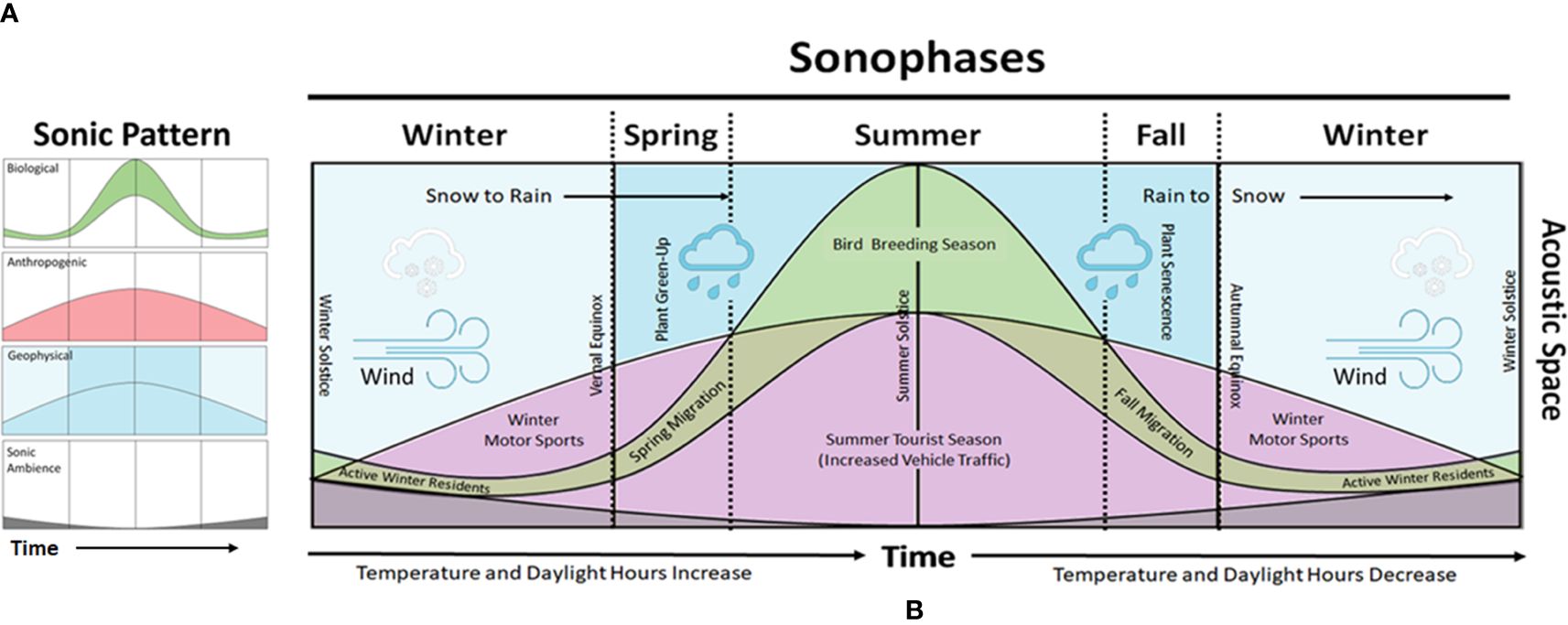
Figure 1 A hypothetical concept model for subarctic sonophases. (A) Patterns emerge from the temporal intensity and frequency distribution of sonic vibrations generated by the Earth's sonic ambience (background sound), geophysical events, biological (animal) behaviors, and anthropogenic (human) activities within the acoustic space. (B) Over time, starting with the winter solstice, temperature and daylight hours begin to increase. A Winter Sonophase may be marked by the geophysical sonic effects of snow and wind that predominantly contribute to the winter soundscape when the low-frequency sounds of animals and intermittent noise from humans (e.g., snowmobiles) abruptly break long periods of sonic ambience. By the vernal equinox, a Spring Sonophase emerges from a reduction in sonic ambience with increasing sonic activity from anthropogenic and biological activities (e.g., increased road traffic and spring songbird migration, respectively) as plants begin to green-up, wind reduces, temperatures increase, and the sonically suppressive influence of snow turns to sonically energetic rainfall. The Summer Sonophase represents the crescendo of sonic activity for the year created by a highly active period of geophysical, biological, and anthropogenic events that peak during the summer solstice. Afterward, a Fall Sonophase emerges as plants shed their leaves simultaneously with a decline in anthropogenic and biological activity coinciding with the closing tourist season and fall songbird migration, respectively. Geophysical activities and sounds become more prominent in the form of rain. The Winter Sonophase returns following the autumnal equinox when temperatures drop below freezing, rain turns to snow, and daylight hours decrease along with the activities of humans and animals.

2 Materials and methods

2.1 Study area and sample site

We focused our sampling efforts within the Exit Glacier Developed Area (EGDA) of Kenai Fjords National Park (KEFJ) located on the Kenai Peninsula of south-central Alaska (Figure 2). Our sample site was situated in a deglaciated (since 1917) maritime rainforest of the Exit Glacier valley. The vegetative community is in transitional succession made up of a forb-grass-fern-lichen understory; a mid-story of Sitka alder (Alnus viridis ssp. sinuata) and willow (Salix sp.); and a canopy consisting of Kenai birch (Betula kenaica), black cottonwood (Populus balsamifera ssp. trichocarpa), Sitka spruce (Picea sitchensis), and mountain hemlock (Tsuga mertensiana). Temperatures range from −30 to 4°C (November–April) and 10 to 25°C (June–August) (PAWD weather station Seward, Alaska; https://mesowest.utah.edu/). Average annual precipitation is 188.3 cm with average annual snow depth (November–May) ranging from 8.7 to 89.1 cm (PAWD weather station Seward, Alaska; https://mesowest.utah.edu/). Monthly wind speeds average 19 km/h in January and decline to a mean low of 10 km/h in July before increasing again through October–November (https://uaf-snap.org).

Figure 2

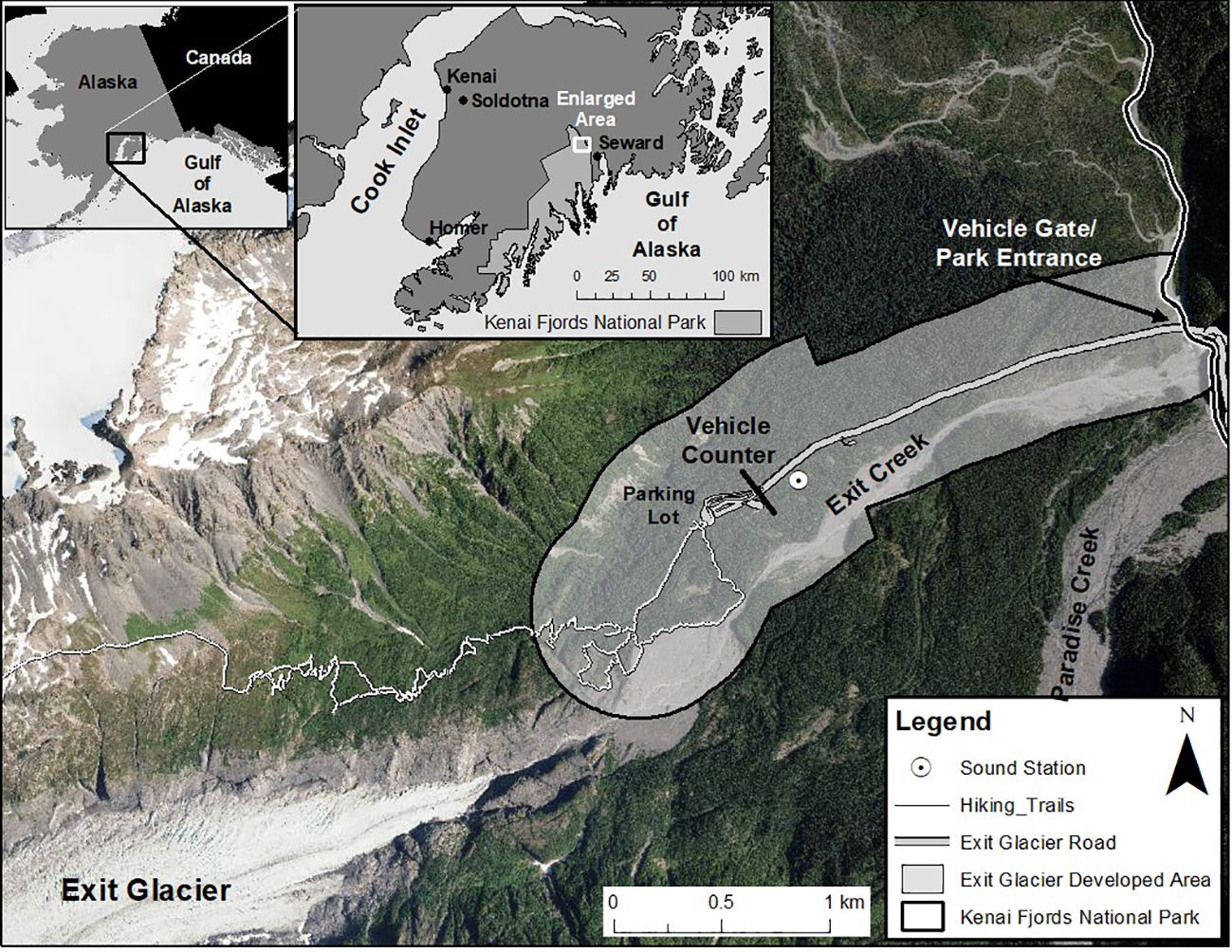
Figure 2 Geographic orientation of the sound recording station and vehicle counter within the Exit Glacier Developed Area of Kenai Fjords National Park in south-central Alaska in relation to human development features, Exit Glacier (in 2019), the outwash plain of Exit Creek, and vehicle gate entrance.

Our sample site was located at 400 m elevation (60.189765°N, 149.623038°W), approximately 1.9 km east from the terminus of Exit Glacier (as of 2021), 190 m northwest from Exit Creek, and 75 m southeast of Exit Glacier Road (Figure 2). The nearby Exit Glacier has retreated rapidly in the last 10 years, receding an average of 50 m/year (unpubl. data). Seasonally, the Exit Glacier Valley is generally subjected to a long winter (November–April) and a short spring (May), summer (June–August), and fall (September–October). During winter, Exit Creek is most often frozen, and the valley is snow-covered with depths ≤2 m as early as late October (unpubl. data) (Supplementary Figure S1). In spring, water in Exit Creek is largely subsurface and snowmelt and green-up proceed slowly as temperatures fluctuate from >0°C during the day and <0°C at night (Supplementary Figure S1). By early summer, vegetation is fully leafed-out and water flow in Exit Creek is highly variable and dependent on ice melt from Exit Glacier, snowmelt from the surrounding mountain peaks, and rain runoff (Supplementary Figure S1). In the fall, water is largely sourced from rainfall and much of it is absorbed into subsurface channels (Supplementary Figure S1) or flows into the Resurrection River and out to Resurrection Bay and the northern Gulf of Alaska.

The road into the EGDA is closed to road-based motor vehicles (e.g., cars, trucks, motorcycles) in winter but is open to non-motorized winter sports (e.g., cross-country skiing, fat tire biking, snowshoeing) and over-snow motor vehicles (e.g., snowmobiles, snow coaches). The gate for road-based motor vehicles is typically open during the tourist season between May and October. The exact date the gate is opened is dependent on snow and road conditions in spring and often varies from year to year. Since 2009, and prior to our study, visitation to KEFJ was increasing 5.6% (SD = 1.7) per year; over 99% of that visitation occurred between the months of May and October (https://irma.nps.gov/STATS/Reports/Park/KEFJ).

2.2 Data acquisition

2.2.1 Soundscape sampling

We deployed a single SM4 Song Meter (Wildlife Acoustics, Inc., Maynard, MA; https://www.wildlifeacoustics.com/images/product_brochures/WA_Brochure_SM4.pdf) 30 m from the Exit Glacier SNOTEL (i.e., snowpack telemetry) weather station (number 1092) (60.189536°N, 149.622811°W). The SM4 recorded the ambient sonic environment in right-channel, mono-aural, at a sample rate of 22,050 Hz for a useable frequency range up to 11,025 Hz. Sounds were recorded for five minutes at one-hour intervals for a total of 120 minutes/day. Microphones were calibrated by the manufacturer to the default sound pressure level of 94 dB with a 10 dB gain and 26 dB preamp. We mounted the sound recorder to the trunk of a Kenai birch tree (40 cm diameter at breast height) at a height of approximately 3 m above the ground to prevent it from being buried in snow (Supplementary Figure S2). We mounted the recorder in a way that positioned the microphone approximately 10 cm from the trunk of the tree to minimize obstructing the microphone’s field of detection (Supplementary Figure S2). The recorder was located in a wooded area to protect the microphone from intense direct wind events that often occur in open and exposed areas (T.C. Mullet, pers. obs.). We used the standard stock foam microphone cover to reduce wind disturbance on the microphone’s surface (https://www.wildlifeacoustics.com/images/product_brochures/WA_Brochure_SM4.pdf). Sound data were saved to 32 GB SD cards in WAV audio format and archived to KEFJ’s sound database.

We visited the recorder at least once a month to retrieve data, change batteries, and conduct any required maintenance. While we intended to record the soundscape continuously from 00:00, 01 January 2019 to 23:00, 31 December 2021, field schedule conflicts in July, August, and September and reduced personnel capacity and bad weather during the months of October, November, and December caused a significant loss of data. This made it impractical to assess the soundscape from July to December for all three sample years. However, sound data were acquired without interruption from 00:00, 01 January to 23:00, 30 June for three consecutive years (2019, 2020, and 2021). Consequently, our study was constrained to the seasonal periods of winter (January–April), spring (May), and early summer (June). Because 2020 was a leap year, we standardized the number of calendar days (CD) across all three years to CD001–CD181.

2.2.2 Phenological climate-related variables

We used climate-related covariates commonly associated with phenology (Schwartz, 2003; Denny et al., 2014) that included: solar photoperiod (hours of daylight from sunrise–sunset), average daily temperature (°C), precipitation (cm), average daily relative humidity (%), daily snow depth (cm), dates when leaves are visibly present on vegetation (i.e., green up), dates when snow cover is no longer visible (i.e., snow-free days), dates when dawn songbird chorus is prevalent (i.e., dawn biophony), and tourism vehicle numbers (vehicles/day). Solar photoperiod was obtained from https://sunrise-sunset.org/us/seward-ak. Temperature, precipitation, relative humidity, and snow depth were acquired from the aforementioned Exit Glacier SNOTEL weather station near our sound recording site. Weather data were accessed from the Natural Resource Conservation Service National Water and Climate Center (https://wcc.sc.egov.usda.gov/nwcc/site?sitenum=1092&state=ak). The start date of green-up and start date of first snow-free days were identified from photographs taken at the Exit Glacier SNOTEL phenocam (https://phenocam.sr.unh.edu/webcam/sites/exglsnotel/, Seyednasrollah et al., 2019).

We knew the dawn chorus made by resident songbirds on the Kenai Peninsula began sometime between March and April (Mullet et al., 2016) and migrant songbirds followed suit by June (Mullet, 2020). Hence, we conducted visual and audio spectrogram analysis in Audacity^® 2.4.1 (https://www.audacityteam.org/) of all sound recordings that were collected between 00:00 and 08:00 from 01 March to 30 June (CD060–CD181) for each sample year (1098 recordings/year). We visually compared spectrograms and identified the first day when the dawn songbird chorus occurred consistently every morning (Supplementary Figure S3).

As a measure of tourism, we counted the number of vehicles entering the EGDA with a magnetic Omega X3 Timestamp Traffic Classifier/Counter (Diamond Traffic Products, Oakridge, OR). The counter detected the axles of vehicles that passed over detection tubes laid across the road where one count is tallied per every two axle detections. The vehicle counter was located at the east-end of the EGDA parking lot within the single-lane entrance (Figure 2). This provided a conservative estimate of vehicle traffic entering, but not exiting, the EGDA. We installed the traffic counter a day prior to Exit Glacier Road opening for public vehicle use. Data were stored on an analog counter and downloaded as a csv file once a month by a KEFJ park ranger.

2.2.3 Acoustic index

We used the Acoustic Complexity Index (ACI) (Pieretti et al., 2011), ACI_tf, after Farina et al. (2016) and Farina and Li (2022) as the quantifiable measure of sonic activity within a recording given a frequency range of 129–11,025 Hz. The ACI is known to be one of the most powerful and effective acoustic indices in Ecoacoustics for analyzing the ecological qualities and relationships of biophony (Alcocer et al., 2022) and low frequency geophony and anthropophony (Farina et al., 2021) in a soundscape (Farina et al., 2023; Farina and Mullet, 2024). Therefore, we expected using ACI as a singular index to test our hypothesis would produce accurate and defensible results. Indices were generated using SonoScape™, an open access software operating in MATLAB which calculated ACI_tf at 1-second intervals for each 5-minute recording across 512 frequency intervals separated at 21.533 Hz intervals (Farina and Li, 2022). We applied an intensity filter to the Fast Fourier Transform (FFT) matrix to exclude values <0.01 that were generated by internal microphone noise.

2.3 Data analysis

2.3.1 Phenological climate-related variables

We calculated the annual averages and 95% confidence intervals (CI) for daily air temperature (°C), relative humidity (%), precipitation (cm), snow depth (cm), and number of vehicles. We also counted the number of days above freezing (>0°C) and identified the calendar day for the following climate-related events (defined in Table 1): vernal equinox (i.e., 12 hours of daylight and 12 hours of night), first day of consecutive days with temperatures >0°C, first day of consecutive snow-free days, first day of green-up, first day of consecutive days of a dawn songbird chorus, and first day of consecutive days when vehicles related to tourism were detected. Vehicle counts of ≤20 vehicles/day within the first three days of the gate being opened were associated with national park service staff activities and not counted (T.C. Mullet per obs.).

Table 1

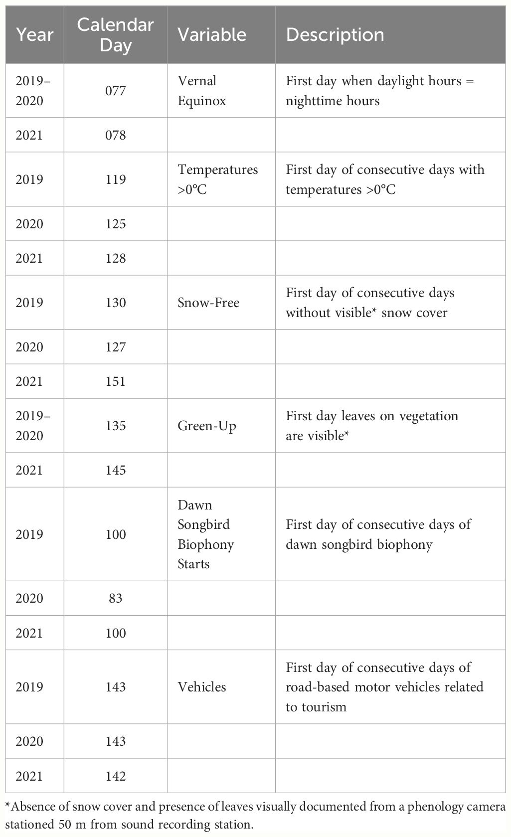
Table 1 Description of climate-related variables, their calendar day and year of occurrence, used to identify phenological relationships with the sonic environment.

2.3.2 Interannual variation and temporal sonic patterns

We calculated the average ACI_tf across the frequency range of 500–7,000 Hz for each sound recording. We selected the lower frequency limit of 500 Hz with the intention of removing sound events that may have been caused by low-frequency turbulence made by wind or vibrations of the sound recorder against its tree mount. Similarly, Mullet et al. (2016) and Mullet (2020) have found that many of the sounds that contribute to the winter, spring, and summer soundscapes typically do not exceed 7,000 Hz, except for the little brown myotis (Myotis lucifugus) that calls above 11,050 Hz (Mullet et al., 2021).

For descriptive purposes, we compared the 95% CI of ACI_tf to determine the extent of interannual variation in sonic activity between years. We visualized the temporal patterns of average ACI_tf over calendar days (CD001–CD181) for the entire sample period of each year. These graphs served as a timeline where we marked the calendar day that each climate-related event (Table 1) began in order to visualize how they compared in association with the temporal patterns of ACI_tf of each sample year.

2.3.3 Sonic-climate relationships

We employed the machine learning algorithm, TreeNet^® Regression (i.e., stochastic gradient boosting) (Friedman, 2002), in the Predictive Analytics Module of Minitab^® 21.2 (Minitab, LLC. State College, PA) to identify the relationships between ACI_tf and climate-related variables (https://support.minitab.com/en-us/minitab/help-and-how-to/statistical-modeling/predictive-analytics/how-to/treenet-regression/before-you-start/overview/). Given that our climate data were inherently interrelated, TreeNet is a powerful statistical and appropriate tool for these datasets because it automatically considers the intricate interaction between predictor variables at each iteration of the model with a pre-assigned cross validation (Friedman, 2002). If a variable is quantified as an important predictor of ACI_tf, variables that are closely related will also be considered (Craig and Huettmann, 2009). Machine learning is highly effective for assigning variable importance in a way that accounts for interactions despite the number of interacting variables (Craig and Huettmann, 2009). For this reason, TreeNet made more practical sense than trying to apply our data within the rule constraints of a general linear model or an information theoretical approach that penalizes a model for having numerous combinations of interacting covariates (Huettmann et al., 2018).

We used six continuous predictor variables: hours of daylight (sunrise to sunset), temperature (°C), snow depth (cm), relative humidity (%), precipitation (cm), and vehicle count with three categorical variables: green leaves (present/absent), snow cover (present/absent), and dawn songbird chorus (present/absent). We developed our model with the following settings: Squared Error Loss Function, 10-Fold Cross-Validation, 0.001 Learning Rate, 0.5 Subsample, 6 Terminal Nodes/Tree with a Minimum Terminal Node Size of 3, and 5,000 Trees. We used the “Discover Key Predictors” function because it produces the best model by starting with all predictor variables then systematically eliminating unimportant predictors until a maximum R-squared value was reached (https://support.minitab.com/en-us/minitab/20/help-and-how-to/statistical-modeling/predictive-analytics/how-to/treenet-regression/before-you-start/overview/).

The Predictive Analytics Module generated a relative variable importance table for our predictor variables that ranks how important subsequent variables are relative to the most important predictor variable. In this way, the most important variable predicting ACI_tf is given a value of 100% and all subsequent variables are ranked by the percent improvement they contribute to predicting ACI_tf (Mizumoto, 2023, https://support.minitab.com/en-us/minitab/20/help-and-how-to/statistical-modeling/predictive-analytics/how-to/treenet-regression/interpret-the-results/relative-variable-importance-chart/). We protected our model from a biased selection of variable importance by selecting the default subsample criteria that randomly selects a proportion of test data without replacement (Minitab, 2018). According to Strobl et al. (2007), machine learning models can avoid biasing their variable importance selection by applying a test data set with a subsample without replacement. This results in a reliable selection of variable importance when predictor variables vary in scale or their number of categories.

We generated two-predictor partial dependence plots in the Predictive Analytics Module for the top climate variables to visualize their interactions in relation to ACI_tf (https://support.minitab.com/en-us/minitab/20/help-and-how-to/statistical-modeling/predictive-analytics/how-to/treenet-regression/interpret-the-results/partial-dependence-plots/).

2.3.4 Sonophase determinations

We determined sonophases during our study period based on our definition that “a sonophase can be defined as a discrete period of prominent or subtle ecological sonic activity that corresponds with the seasonality of distinct geophysical, biological, and anthropogenic events that are associated with changes in climate.” Accordingly, ACI_tf served as our measure of “ecological sonic activity” that occurred between the frequencies of 500 and 7,000 Hz. Our temporal periods included the calendar days CD001–CD181 over three sample years (2019–2021). We distinguished sonophases through a stepwise process.

To find how ACI_tf “corresponds with the seasonality of distinct geophysical, biological, and anthropogenic events that are associated with changes in climate,” we first identified the ACI_tf values associated with the exact calendar day and period of occurrence for our seasonal climate-related events described in Table 1. Second, we categorize ACI_tf based on the start and end dates for climate-related events described in Table 2, referencing our conceptual model (Figure 1). Third, we calculated and compared 95% CI of ACI_tf values representing the categories described in Table 2 and distinguished discrete sonophases if 95% CI did not overlap. Finally, we verified the distinctiveness of sonophases over our entire sample period by comparing the 95% CI of each sonophase within each sample year. We visualized the temporal patterns of ACI_tf across calendar days in association with their respective sonophases by sample year and averaged across all three years. We visualized and described the patterns of ACI_tf (averaged over all three years) for each sonophase according to hourly intervals of a 24-h day.

Table 2

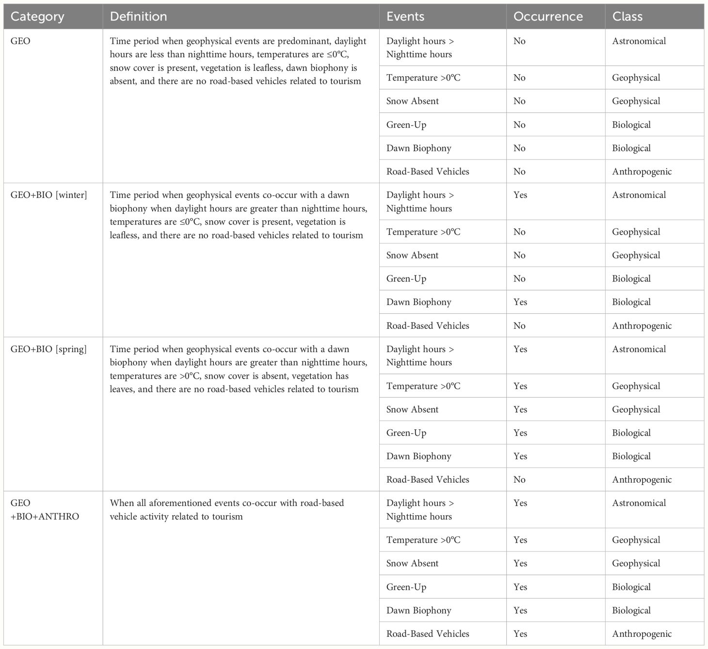
Table 2 Definitions for categories of climate-related events occurring 01 January–30 June.

Essentially, we split ACI_tf values into categories and time periods when specific climate-related seasonal events occurred (presented in Table 1 and defined in Table 2). This approach allowed us to determine if sonic activity (ACI_tf), grouped according to specific, climate-related phenological events, expressed distinct, statistically significant differences. If so, then the appearance of sonic activity distinguished between groups would reveal discrete sonic phases (i.e., sonophases) linked to seasonal events affected by climate. We assumed that if sonic activity (ACI_tf) could not be statistically distinguished by comparing 95% CI between distinct groups of climate-dependent phenological events, then the temporal patterns of ACI_tf were not linked to these commonly measured and utilized phenology and climate metrics.

3 Results

3.1 Data capacity and processing

We gathered a total of 13,056 five-minute recordings from 01 January–30 June 2019, 2020, and 2021, making up 160 GB of data. Although 2020 was a leap year, we utilized a standard data set across calendar days for all years that included 4,344 recordings for each sample year (CD001–CD181). Our processing time to acquire acoustic indices through the SonoScape™ software required 12 hours for each year’s worth of data.

3.2 Phenology of climate-related variables

There was significant interannual variation of climate-related weather data from January and June with no single variable being consistent among all three years of sampling. Average daily air temperature in 2019 ($\overline{X}=$ −0.4°C; 95% CI: −0.6 to 1.4) was significantly higher than 2020 ($\overline{X}=$ −2.9°C; 95% CI: −4.2 to −1.4) and similar to 2021 ($\overline{X}=$ −1.6°C; 95% CI: −2.7 to −0.5) (Supplementary Table S1). However, 2019 had 108 days of above-freezing temperatures (>0°C) while 2020 and 2021 had 83 and 85 days of above-freezing temperatures, respectively. Precipitation was significantly higher in 2019 ($\overline{X}=$ 133.1 cm; 95% CI: 131.2–135.2) than 2020 ($\overline{X}=$ 124.0; 95% CI: 122.2–125.7) but both years were significantly lower than 2021 ($\overline{X}=$ 170.1; 95% CI: 165.7–174.6) (Supplementary Table S1). Relative humidity was higher in 2019 ($\overline{X}=$ 87.6%; 95% CI: 86.1–89.1) than subsequent years but similar between 2020 ($\overline{X}=$ 81.6; 95% CI: 79.7–83.4) and 2021 ($\overline{X}=$ 83.9; 95% CI: 81.9–85.8) (Supplementary Table S1). Snow depth was similar between 2019 ($\overline{X}=$ 37.0 cm; 95% CI: 32.7–41.4) and 2020 ($\overline{X}=$ 39.2 cm; 95% CI: 34.0–44.4) but significantly higher in 2021 ($\overline{X}=$ 111.2 cm; 95% CI: 101.0–121.3) (Supplementary Table S1). By September 2019, the Kenai Peninsula, including our study area, was classified as being in severe drought (https://droughtmonitor.unl.edu/).

The day when temperatures were consistently >0°C began on CD119 (29 April) in 2019, CD125 (04 May) in 2020, and CD128 (08 May) in 2021 (Table 1). Snow cover was present at the start of our sample period on CD001 (01 January) for all three years (Table 1). Snow-free days began on CD130 (10 May) in 2019, CD127 (06 May) in 2020, and CD151 (31 May) in 2021 (Table 1). Green-up of vegetation was first detected on black cottonwood and Kenai birch for all three years and started on CD135 (15 May) in 2019, CD135 (14 May) in 2020, and CD145 (24 May) in 2021 (Table 1). Compared to 2019 and 2020, snow cover remained approximately 18% longer and green-up started 10 days later in 2021.

Songbirds, specifically flocks of common redpoll (Acanthis flammea) and varied thrush (Ixoreus naevius), two common winter residents, began singing consistently every morning at dawn (06:00–07:00) on CD100 (10 April) in 2019, CD83 (23 March) in 2020, and CD100 (10 April) in 2021 (Table 1). The park gate was opened to motor vehicles on CD143 (23 May) of 2019, and CD140 (20 May) of 2020, and CD139 (18 May) of 2021 (Table 1). Tourist-related vehicle activity began on CD143 (23 May) of 2019, CD143 (22 May) of 2020, and CD142 (22 May) of 2021. By these times, resident and migratory songbirds were already calling consistently from 03:00 to 22:00 daily in all three years. Vehicle traffic following the gate opening averaged 89.2 vehicles/day (95% CI: 60.9–117.4) in 2019, decreasing significantly to 41.4 vehicles/day (95% CI: 28.3–54.4) in 2020, and then rising dramatically to 115.0 vehicles/day (95% CI: 82.3–147.6) in 2021 (Supplementary Table S1).

Although KEFJ had been experiencing an average annual increase of 5.6% (SD = 1.7) visitors over the past decade, visitation during the onset of the novel coronavirus SARS-CoV-2 (COVID-19) pandemic in 2020 dropped by nearly 68% from the previous year. In 2021, visitor numbers increased by nearly 250% (n = 411,782) from those of 2020 (n = 115,882) but only 15% from 2019 (n = 356,601) (https://irma.nps.gov/STATS/Reports/Park/KEFJ).

3.3 Interannual variation and temporal sonic patterns

We found remarkable differences in ACI_tf when visualized over calendar days for each sample year in relation to the timing of climate-related events (Figure 3). Prior to the vernal equinox, we observed an intermittent occurrence of nine significant peaks in sonic activity in 2019, three in 2020, and five smaller but noticeable peaks in 2021 all attributed to rain events during our study period (Figure 3). These peaks in sonic activity were contrasted sharply by long periods of significantly low ACI_tf values ranging from 8 to 12 days in 2019, 7 to 46 days in 2020, and 2 to 22 days in 2021. Following the vernal equinox, ACI_tf peaks occurred more frequently than earlier periods of each year as sonic activity notably increased in concert with longer daylight hours, the start of the dawn songbird chorus, and consecutive days above freezing for all three years (Figure 3). Days of lower ACI_tf following the vernal equinox were comparably fewer than those documented prior to it. Sonic activity continued to increase significantly with an increasing number of climate-related events including consecutive snow-free days, the start of green-up, continued presence of a dawn songbird chorus, and the first influx of road-based motor vehicles related to tourism (Figure 3).

Figure 3

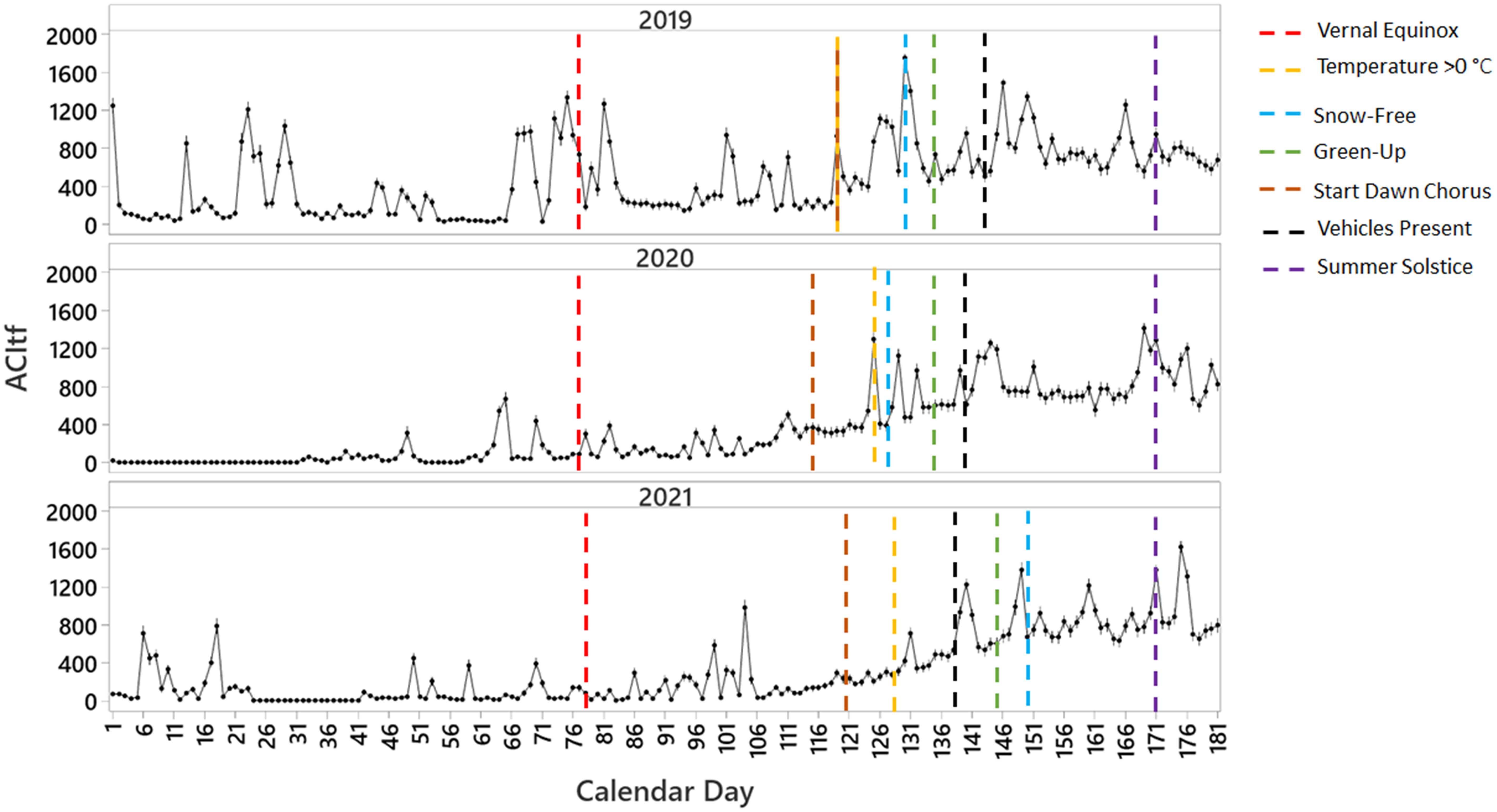
Figure 3 Average sonic activity (ACI_tf) over calendar days (01 January = 001 to 30 June = 181) across three years of sampling in relation to the vernal equinox, summer solstice, and the calendar day when climate-related events began.

3.4 Sonic-climate relationships

Our best fit model was reached at 4997 trees with R² values of 82.12% for the training dataset and 70.27% for the test (predictive) dataset (Supplementary Table S2). The ACI_tf was strongly related to the following climate-related variables, ranked in order of importance: temperature (100%), hours of daylight (60%), snow depth (49%), relative humidity (37%), and precipitation (31%) (Supplementary Table S2). Specifically, sonic activity of the soundscape increased with warmer days, especially >0°C, that coincided with longer daylight hours and shallow or no snow (Supplementary Figure S4). The lowest ACI_tf values coincided with colder temperatures and darker days (Supplementary Figure S4). The soundscape also exhibited relatively greater values of ACI_tf when RH was<60% and >90%, co-occurring with no and high precipitation, respectively (Supplementary Figure S4). Categorical predictor variables of green leaves (present/absent), snow cover (present/absent), and dawn songbird chorus (present/absent) were omitted during model iterations because they did not appreciably add to the model’s predictive accuracy (https://support.minitab.com/en-us/minitab/20/help-and-how-to/statistical-modeling/predictive-analytics/how-to/treenet-regression/before-you-start/overview/) (Supplementary Table S2).

3.5 Sonophases

We found, with 95% confidence, that when ACI_tf was grouped into categories based on the seasonal occurrence of distinct climate-related events, the soundscape exhibited four temporally discrete sonophases. This included two winter sonophases (Sonophase I and Sonophase II), a spring sonophase (Sonophase III), and a summer sonophase (Sonophase IV) that occurred successively from 01 January (CD001) to 30 June (CD181) (Table 3). Based on a three-year average, Sonophase I occurred from CD001 to CD099, during the darkest and coldest days that transpired over our sample period (Figure 4). Sonophase I expressed the lowest ACI_tf values ($\overline{X}=$ 169.75, 95% CI: 167.0–172.5) than all other sonophases (Table 3). Sonophase II expressed relatively low, but significantly greater ACI_tf values than Sonophase I ($\overline{X}=$ 243.99, 95% CI: 238.9–249.1) (Table 3) between CD079 and CD119, marked prominently by the onset of a dawn resident songbird chorus when daylight hours began to increase but temperatures remained predominantly below freezing, snow cover persisted, vegetation remained leafless, and human activities (e.g., snowmobiling) were minimal (Figure 4). The interannual overlap of Sonophase I and II were caused by interannual variations in the start dates of the dawn resident songbird choruses which started 17 days earlier in 2020 (CD83) than in 2019 (CD100) and 2021 (CD100). Significant peaks in ACI_tf during Sonophase I and II were predominantly associated with intermittent days with temperatures above freezing, often cooccurring with rain events (Figure 4). Averaged over all three years, Sonophase I had proportionally fewer days above freezing with concurrent rain events ($\overline{X}=$ 0.19, SD = 0.08) than Sonophase II ($\overline{X}=$ 0.46, SD = 0.03).

Table 3

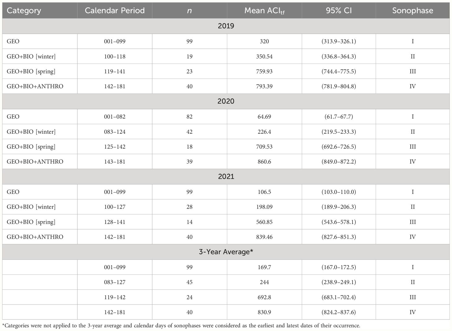
Table 3 Calendar period, number of days (n), mean index of sonic activity (ACI_tf) and 95% confidence intervals (CI) with their sonophase Roman numeral based on non-overlapping 95% CI.

Figure 4

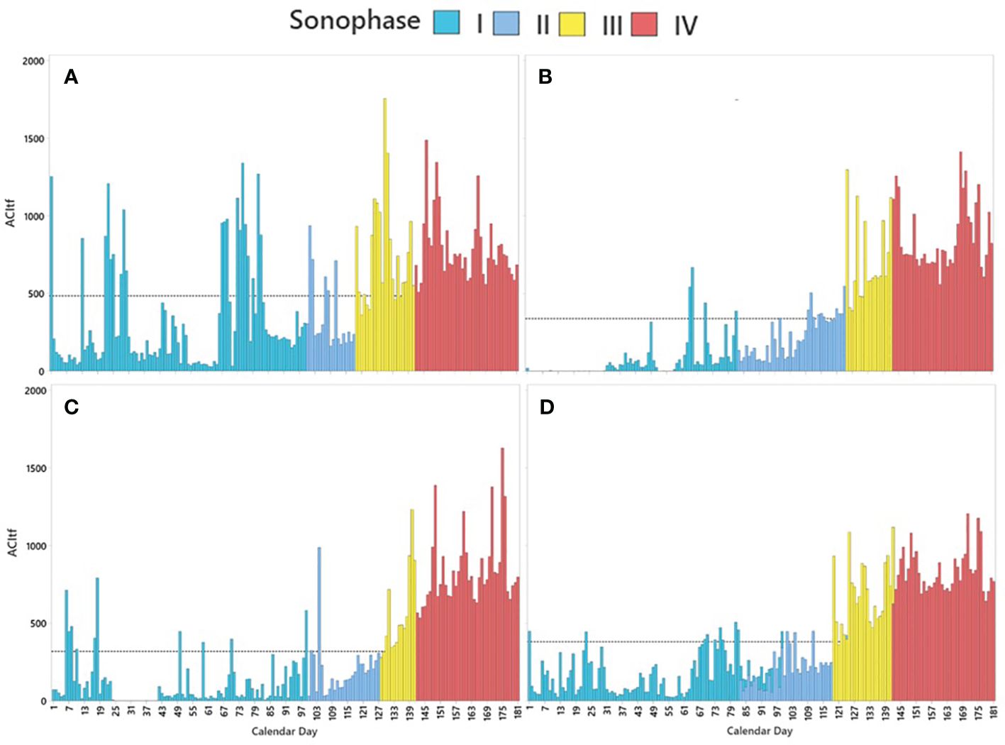
Figure 4 Temporal patterns of average sonic activity (ACI_tf) expressed as four statistically distinct sonophases over calendar days 001 (01 January) to 181 (30 June) in (A) 2019, (B) 2020, (C) 2021, and (D) averaged over all three years. The black dotted line represents annual average ACI_tf for 2019 ($\overline{X}=$ 483.72, 95% CI: 478.56–488.89), 2020 ($\overline{X}=$ 337.72, 95% CI: 333.21–342.22), 2021 ($\overline{X}=$ 317.79, 95% CI: 313.37–322.22), and average over all three years ($\overline{X}=$ 379.75, 95% CI: 377.01–382.49). Days with prominent spikes in average ACI_tf are indicative of rain events.

Sonophase III expressed significantly greater ACI_tf values ($\overline{X}=$ 692.76, 95% CI: 683.1–702.4) than Sonophase I and II, occurring between CD119 and CD142 (Figure 4). Sonophase III coincided with longer periods of daylight, consecutive days with temperatures above freezing, the timing of green-up, and a daily dawn songbird chorus (starting at 03:00) consisting of both resident and migrant species, and minimal to no human activity due to degrading snow conditions for winter recreation (Figure 4). Sonophase IV began on CD142 within days of the vehicle gate opening to the park. Sonophase IV expressed the highest values of ACI_tf than all previous sonophases ($\overline{X}=$ 830.89, 95% CI: 824.2–837.6) (Table 3) coinciding with the longest and warmest days of the year, a diverse dawn songbird chorus of resident and migrant species, and the onset and daily prevalence of road-based motor vehicles related to tourism. Sonic activity seemingly peaked around the summer solstice (CD171) and subtly declined to the end of our sample period (CD181) except for peaks in ACI_tf during rainy days (Figure 4). Sonophases remained statistically distinct and expressed similar characteristics as those described above when average ACI_tf and 95% CI were compared within individual sample years (Table 3).

Values of ACI_tf exhibited differential patterns at hourly intervals when visualized over a 24-h day by sonophase. Over winter, ACI_tf values of Sonophase I were significantly lower than other sonophases, exhibiting marginal fluctuations of relatively higher values between 23:00 – 03:00 with a noticeable rise between 10:00 and 14:00 (Figure 5). Sonophase II expressed marginally higher ACI_tf values with a subtle rise in sonic activity at 07:00, when dawn songbird biophony was evident, then showing a noticeable peak at 13:00 (Figure 5). Sonic activity dramatically increased during Sonophase III with distinct peaks in ACI_tf between the hours of 03:00 and 08:00, coinciding with dawn songbird biophony, then subsequently declining throughout the day (Figure 5). While a dawn songbird biophony was still evident at 03:00 and 04:00, Sonophase IV exhibited its most significant peak in ACI_tf between the hours of 11:00 and 17:00. This peak coincided with the peak in motor vehicle-based tourism indicating a significant contribution of anthropophony to this soundscape in summer. Notably, the lowest ACI_tf values of Sonophase IV occurred during 23:00–02:00 when human and animal activities we at their minimum (Figure 5). The particularly low baseline values of ACI_tf during Sonophases I and II were predominantly attributed to geophony originating from prolonged periods of subtle and distant wind events in the near absence of biophony and anthropophony. In contrast, the significantly higher baseline values of ACI_tf that were evident during Sonophases III and IV were attributed to the continuous geophony produced by the sound of flowing water of the nearby Exit Creek produced by rain runoff and the melting of Exit Glacier and snow from the surrounding mountain peaks.

Figure 5

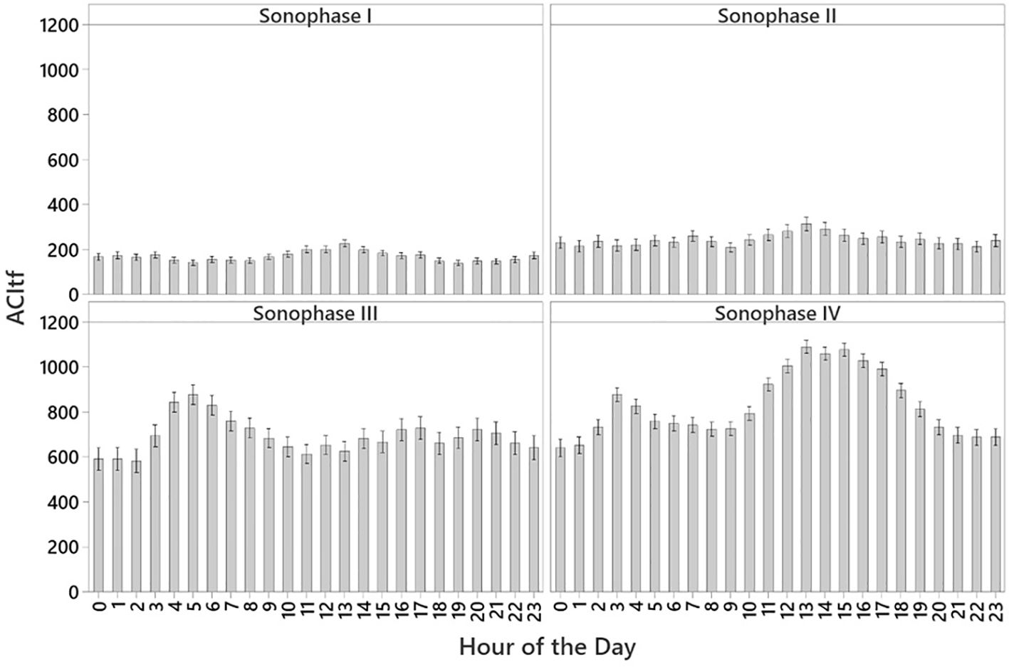
Figure 5 Temporal patterns of ACI_tf of four discrete sonophases averaged by hour over a 24-h day with 95% confidence intervals.

4 Discussion

As we expected, sonic activity increased from winter to summer with rising temperatures, longer daylight hours, and diminishing (melting) snow cover that appropriately coincided with songbird breeding behavior and tourist activity (Slagsvold, 1977; Amelung et al., 2007). The phenological patterns we observed in the land- and soundscape were directly related to the seasonal shifts in climatic conditions that occur in this part of Alaska. Consequently, sonic activity was generated by sequential and compounding sound-producing physical events that occur in time with seasonal climate conditions (Schwartz, 2003; Denny et al., 2014) (Figure 1).

Complimentary to our model’s prediction, we revealed a distinct Sonophase I that expressed the lowest ACI_tf values of the year during days averaging<9 h and 40 min of daylight, daily temperatures predominantly below freezing, a prominent snowpack, and extremely minimal animal and human activity. At this time of year, biophony and anthropophony in the soundscape are near absent and intermittent periods of geophony from wind are replaced by a sonic environment so reduced in intensity, on somedays, it can be hard to measure with scientific instruments (Mullet, 2014; Mullet et al., 2016). While humans refer to this phenomenon as natural quiet (Mullet et al., 2017), what is ecologically revealed at this time is the fundamental acoustic niche filled by the baseline (background) sonic activity of Earth, referred to in Ecoacoustics as the sonic ambience (Farina et al., 2021). The sonic characteristics of Sonophase I epitomizes those of winter in this subarctic region of Alaska (Mullet et al., 2016).

We unexpectedly discovered a second winter sonophase (Sonophase II) that was statistically evident over calendar days within years and when averaged over all three years. We were able to categorically distinguish Sonophase II from Sonophase I by the presence of a distinct beginning and sequential days of a dawn resident songbird chorus that occurred during days with longer daylight hours following the vernal equinox. It is also likely that the higher proportion of days with temperatures above freezing, and their associated rain events, also contributed to the prominence of a second winter sonophase. Although interesting, we suspect that a second winter sonophase may be more intimately related to our study area than other subarctic ecosystems of south-central Alaska. The Exit Glacier Developed Area is dryer than its coastal glacier counterparts on the eastern Kenai Peninsula (Helm and Allen, 1995) and wetter than the spruce-dominated landscapes of the west (Magness and Morton, 2018). However, because winter is still the longest season of the year in this region, we encourage further study into winter sonic patterns and potentially spatial difference in sonophases.

Although we conceptualized the start of a spring sonophase in Figure 1 to follow the vernal equinox, our results revealed a distinct sonophase later in the year but still coinciding with seasonal events commonly demarcating spring. Sonophase III exhibited a significant and dramatic increase in ACI_tf that coincided with the beginning of consecutive calendar days above freezing, the start of green up, no snow cover, and a prominent dawn chorus comprised of a resident and migrant songbird community. Spring has been a focus for investigating indicators of climate change in the subarctic ecosystems of Alaska. Studies have found in some parts of Alaska that snow melt is occurring earlier in spring (Stone et al., 2002). Similar events have been observed to predominate advances in vegetation green up (Zheng et al., 2022). There is even some evidence that spring biophony and songbird phenology are being affected by climate change in Alaska (Buxton et al., 2016; Oliver et al., 2020). Although we cannot claim these effects from our results, we do provide the first evidence that the soundscape, in its entirety, exhibited distinct changes according to climate conditions that coincide closely with the climate-effected variables investigated by these other studies.

The emergence of Sonophase IV in summer was an important phenological period because it was distinguished from Sonophase III specifically by the onset and continuity of road-based motor vehicles related to tourism and the anthropophony it generated. We suspect that the start of Sonophase IV and the duration of Sonophase III in our study area could be greatly altered in the future if snow conditions along Exit Glacier Road change with the warming conditions expected for this area of the Kenai Peninsula (Hayward et al., 2017). Although the superintendent of KEFJ usually opens the vehicle gate about one week before the last Monday in May (i.e., Memorial Day holiday in the U.S.A.), pressure from the public to open the vehicle gate earlier occurs every year (J.W. Carroll, KEFJ Superintendent, pers comm.). Since the snow removal of Exit Glacier Road is dependent on the schedule of the Alaska Department of Transportation, KEFJ usually must wait for their decision and a snow-free road to do so. However, if predictions are accurate, the Exit Glacier Developed Area could experience warmer springs and earlier start dates of snow-free days (Hayward et al., 2017; Magness and Morton, 2018). If the anthropophony of road-based motor vehicles related to tourism begins significantly earlier, the seasonal sonophases of the Exit Glacier soundscape could be dramatically changed and potentially effect ecological processes. This is not an unusual assumption. In fact, tourist seasons are lengthening due to climate change all over the world (Hyslop, 2007; Albano et al., 2013; Monahan et al., 2016) and soundscapes are being affected (Merchan et al., 2014).

5 Conclusion

We empirically identified four discrete sonophases that occurred between January and June in this subarctic ecosystem of Kenai Fjords National Park. We found evidence that these sonophases emerged because the seasonal patterns of the soundscape coincided intricately with the phenological phases of distinct climate-dependent geophysical (e.g., temperature, precipitation, snow cover) (Schöner et al., 2009; Bojinski et al., 2014), biological (e.g., dawn songbird chorus, green up) (Buxton et al., 2016; Oliver et al., 2018), and anthropogenic (e.g., vehicle traffic from tourism) (Amelung et al., 2007) events as winter transitioned to summer. This ecological relationship was further supported by our TreeNet model that revealed how the soundscape was linked to the seasonality of concurrent weather data collected at a nearby weather station. These results provide strong support for the Sonophenology Hypothesis and its application to the phenological studies of climate change.

The effects of human-caused climate change are already here on the Kenai Peninsula of Alaska. Mean annual temperature in the adjacent Cook Inlet region has already warmed 0.7°C this century, with winter temperatures (January−February) 1.7°C higher than a century earlier (Shulski and Wendler, 2007:141). Even at a medium emission scenario (RCP 6.0), the forecasted climate for Seward (headquarters to KEFJ) suggests mean temperatures will continue to increase in all months through at least 2099, exceeding 15°C in July and August (https://uaf-snap.org). Predictions of mean monthly precipitation is highly variable through the end of this century, but generally increasing in fall and winter, but not in spring and summer (April−July). Winter (defined by a mean monthly temperature ≤0°C) will decrease from five months (November−March) to two months (December–January) by 2060, suggesting rapidly decreasing snowpack. These warming temperatures translate to a growing season (number of days >4°C) forecasted to increase from three to almost six months by 2099 (https://uaf-snap.org/). Wind events of ≥1 h duration are forecasted to decrease approximately 10% by 2039 and remain stable through 2099 (https://uaf-snap.org). Concomitantly, mean sea level at the Seward Harbor is expected to rise 25 cm by 2050 (https://sealevelrise.org/states/alaska). These environmental changes will inevitably impact the sonophenology of this region.

It is clear that the soundscape in this part of Alaska is sensitive to seasonal climate change and likely sensitive to the effects of human-caused climate change and other environmental disturbances. We think our results provide enough evidence to suggest that the soundscape could serve as a complimentary variable to monitor multi-dimensional ecological processes using ACI_tf along with weather data collected at weather stations around the world. However, there remains opportunities to investigate how other acoustic indices may behave under similar methodologies. In this way, the Sonophenology Hypothesis can be tested in a variety of biomes and ecosystems with an array of ecoacoustic perspectives. Such results are likely to provide ecologists with a systems-based perspective of how human caused climate change is impacting the geophysical, biological, and anthropogenic attributes of our planet. We encourage further study of this novel approach.

Data availability statement

The datasets presented in this study can be found in online repositories. The names of the repository/repositories and accession number(s) can be found below: https://irma.nps.gov/DataStore/Reference/Profile/2294624.

Author contributions

TM: Conceptualization, Data curation, Formal analysis, Funding acquisition, Investigation, Methodology, Project administration, Resources, Software, Supervision, Validation, Visualization, Writing–original draft, Writing–review & editing. AF: Data curation, Formal analysis, Funding acquisition, Resources, Software, Validation, Visualization, Writing–original draft, Writing–review & editing. JM: Writing–original draft. SW: Data curation, Investigation, Validation, Writing–original draft.

Funding

The author(s) declare financial support was received for the research, authorship, and/or publication of this article. This project was funded by the U.S. National Park Service, which helped with personnel, equipment, and software for the research, analysis, and writing of this article.

Acknowledgments

We acknowledge the mentorship and profound support of the late S.H. Gage. We extend a special thank you to R. Benocci and two anonymous reviewers for their support of our work. We thank the Resource Management and Visitor Resource Protection staff of Kenai Fjords National Park who helped with maintaining our sound recorder over the years. We are thankful to S. Gende from the NPS Alaska Regional Office and P. Li for their help and support with data analysis. Thanks to K.F. who challenged us to improve the original manuscript. Special thanks to A. Lyon for her unconditional support. The findings and conclusions in this article are those of the authors and do not necessarily represent the views of any government agencies. Any use of trade, product, or firm names is for descriptive purposes only and does not imply and endorsement by the U.S. government.

Conflict of interest

We declare that our research was conducted in the absence of any commercial or financial relationships that could be construed as a potential conflict of interest.

Publisher’s note

All claims expressed in this article are solely those of the authors and do not necessarily represent those of their affiliated organizations, or those of the publisher, the editors and the reviewers. Any product that may be evaluated in this article, or claim that may be made by its manufacturer, is not guaranteed or endorsed by the publisher.

Supplementary material

The Supplementary Material for this article can be found online at: https://www.frontiersin.org/articles/10.3389/fevo.2024.1345558/full#supplementary-material

Supplementary Figure 1 | Visualization of seasonal changes in the Exit Glacier Valley of Kenai Fjords National Park, Alaska.

Supplementary Figure 2 | SM4 automated acoustic recording device (ARD) used to record ambient sounds at Exit Glacier Developed Area in Kenai Fjords National Park, Seward, Alaska between 01 January and 30 June 2019, 2020, and 2021. The ARD is attached 3- m above ground on a Kenai birch 30 m from a weather station in a post-glaciated (since 1917) subarctic system. Photo was taken by T.C. Mullet 18 June 2019.

Supplementary Figure 3 | An example of spectrograms from seven 2-minute, 30-second subsample recordings at 06:00 between 06 and 12 April 2019. Trained professionals (T.C. Mullet and S.R. Wilhelm) could visually identify there was no songbird activity in spectrograms during 06–09 April 2019 but there were distinct songbird calls from multiple species on 10, 11, and 12 April 2019. We conducted this spectral analysis on recordings in 2019, 2020, and 2021 between the hours of 00:00 and 08:00 from 01 March to 30 June. This method allowed us to determine the exact start date when a dawn songbird chorus occurred regularly on consecutive days each year as an animal behavior associated with seasonal change related to climate. Here, that start date is 10 April 2019 (calendar day 100).

Supplementary Figure 4 | Two-predictor partial dependence plots visualizing the sonic-climate relationship represented by the acoustic complexity index (ACI_tf) and its interaction with climate-related variables of (A) hours of daylight vs temperature, (B) snow depth vs temperature, (C) snow depth vs hours of daylight, and (D) precipitation vs relative humidity.

Supplementary Table 1 | Climate-related variable measures and comparable 95% confidence intervals (CI) by sample year.

Supplementary Table 2 | Model selection to determine the optimum relationship (R²) between the sonoscape (ACI_tf) and climate-related variables. *Optimal model R².

References

Adam J. C., Hamlet A. F., Lettenmaier D. P. (2009). Implications of global climate change for snowmelt hydrology in the twenty-first century. Hydrol. Processes: Int. J. 23, 962–972. doi: 10.1002/hyp.7201

CrossRef Full Text | Google Scholar

Albano C. M., Angelo C. L., Strauch R. L., Thurman L. L. (2013). Potential effects of warming climate on visitor use in three Alaskan national parks. Park Sci. 30, 37–44.

Google Scholar

Alcocer I., Lima H., Sugai L. S. M., Llusia D. (2022). Acoustic indices as proxies for biodiversity: a meta-analysis. Biol. Rev. 97, 2209–2236. doi: 10.1111/brv.12890

CrossRef Full Text | Google Scholar

Amelung B., Nicholls S., Viner D. (2007). Implications of global climate change for tourism flows and seasonality. J. Travel Res. 45, 285–296. doi: 10.1177/0047287506295937

CrossRef Full Text | Google Scholar

Bojinski S., Verstraete M., Peterson T. C., Richter C., Simmons A., Zemp M. (2014). The concept of essential climate variables in support of climate research, applications, and policy. Bull. Am. Meteorol. Soc. 95, 1431–1443. doi: 10.1175/BAMS-D-13-00047.1

CrossRef Full Text | Google Scholar

Buxton R. T., Brown E., Sharman L., Gabriele C. M., McKenna M. F. (2016). Using bioacoustics to examine shifts in songbird phenology. Ecol. Evol. 6, 4697–4710. doi: 10.1002/ece3.2242

PubMed Abstract | CrossRef Full Text | Google Scholar

Craig E., Huettmann F. (2009). Using” Blackbox” Algorithms such AS treeNET and random forests for data-ming and for finding meaningful patterns, relationships and outliers in complex ecological data: an overview, an example using G. Intell. Data anal.: develop. New methodol. through Pattern Discovery recovery, 65–84. doi: 10.4018/978-1-59904-982-3.ch004

CrossRef Full Text | Google Scholar

Denny E. G., Gerst K. L., Miller-Rushing A. J., Tierney G. L., Crimmins T. M., Enquist C. A., et al. (2014). Standardized phenology monitoring methods to track plant and animal activity for science and resource management applications. Int. J. Biometeorol. 58, 591–601. doi: 10.1007/s00484-014-0789-5

PubMed Abstract | CrossRef Full Text | Google Scholar

Farina A., Gage S. H. (Eds.) (2017). Ecoacoustics: The ecological role of sounds (Hoboken, NJ, USA: John Wiley & Sons). doi: 10.1002/9781119230724

CrossRef Full Text | Google Scholar

Farina A., Li P. (2022). Methods in ecoacoustics: the acoustic complexity indices Vol. 1 (Switzerland: Springer Nature).

Google Scholar

Farina A., Mullet T. C., Bazarbayeva T. A., Bulatova D., Tazhibeyva T., Li P. (2021). Perspectives on the ecological role of geophysical sounds. Front. Ecol. Evol., 919. doi: 10.3389/fevo.2021.748398

CrossRef Full Text | Google Scholar

Farina A., Mullet T. C., Bazarbayeva T. A., Tazhibayeva T., Polyakova S., Li P. (2023). Sonotopes reveal dynamic spatio-temporal patterns in a rural landscape of Northern Italy. Front. Ecol. Evol. 11, 1205272. doi: 10.3389/fevo.2023.1205272

CrossRef Full Text | Google Scholar

Farina A., Pieretti N., Salutari P., Tognari E., Lombardi A. (2016). The application of the acoustic complexity indices (ACI) to ecoacoustic event detection and identification (EEDI) modeling. Biosemiotics. 9, 227–246. doi: 10.1007/s12304-016-9266-3

CrossRef Full Text | Google Scholar

Farina A., Mullet T. C. (2024). Sonotope patterns within a mountain beech forest of Northern Italy: a methodological and empirical approach. Front. Ecol. Evol. 12, 1341760.

Google Scholar

Friedman J. H. (2002). Stochastic gradient boosting. Comput. Stat Data Anal. 38, 367–378. doi: 10.1016/S0167-9473(01)00065-2

CrossRef Full Text | Google Scholar

Hayward G. D., Colt S., McTeague M. L., Hollingsworth T. N. (2017). “Climate change vulnerability assessment for the Chugach National Forest and the Kenai Peninsula,” in General Technical Report-Pacific Northwest Research Station, USDA Forest Service. (PNW-GTR-950).

Google Scholar

Helm D. J., Allen E. B. (1995). Vegetation chronosequence near Exit Glacier, Kenai Fjords National Park, Alaska, USA. Arctic Alpine Res. 27, 246–257. doi: 10.2307/1551955

CrossRef Full Text | Google Scholar

Huettmann F., Craig E. H., Herrick K. A., Baltensperger A. P., Humphries G. R., Lieske D. J., et al. (2018). Use of machine learning (ML) for predicting and analyzing ecological and ‘presence only’ data: an overview of applications and a good outlook. Mach. Learn. Ecol. Sustain. Natural Res. Manage., 27–61.

Google Scholar

Hyslop K. E. (2007). Climate change impacts on visitation in National Parks in the United States. (Ontario, Canada: University of Waterloo).

Google Scholar

IPCC. (2021). “Regional fact sheet—Polar regions,” in Climate change 2021: The physical science basis. Eds. Masson-Delmotte V., Zhai P., Pirani A., Connors S. L., Péan C., Chen Y., et al. Available at: https://www.ipcc.ch/report/ar6/wg1/. Contribution of Working Group I to the Sixth Assessment Report of the Intergovernmental Panel on Climate Change.

Google Scholar

Krause B., Farina A. (2016). Using ecoacoustic methods to survey the impacts of climate change on biodiversity. Biol. Conserv. 195, 245–254. doi: 10.1016/j.biocon.2016.01.013

CrossRef Full Text | Google Scholar

Lenzen M., Sun Y. Y., Faturay F., Ting Y. P., Geschke A., Malik A. (2018). The carbon footprint of global tourism. Nat. Climate Change. 8, 522–528. doi: 10.1038/s41558-018-0141-x

CrossRef Full Text | Google Scholar

Lisovski S., Ramenofsky M., Wingfield J. C. (2017). Defining the degree of seasonality and its significance for future research. Integr. Comp. Biol. 57, 934–942. doi: 10.1093/icb/icx040

PubMed Abstract | CrossRef Full Text | Google Scholar

Magness D. R., Morton J. M. (2018). Using climate envelope models to identify potential ecological trajectories on the Kenai Peninsula, Alaska. PloS One. 13, e0208883. doi: 10.1371/journal.pone.0208883

PubMed Abstract | CrossRef Full Text | Google Scholar

Merchan C. I., Diaz-Balteiro L., Soliño M. (2014). Noise pollution in national parks: Soundscape and economic valuation. Landscape Urban Plann. 123, 1–9. doi: 10.1016/j.landurbplan.2013.11.006

CrossRef Full Text | Google Scholar

Miller-Rushing A. J., Lloyd-Evans T. L., Primack R. B., Satzinger P. (2008). Bird migration times, climate change, and changing population sizes. Global Change Biol. 14, 1959–1972. doi: 10.1111/j.1365-2486.2008.01619.x

CrossRef Full Text | Google Scholar

Minitab. (2018). Salford predictive modeler: Introducing TreeNet gradient boosting machine. Available online at: https://acrobat.adobe.com/id/urn:aaid:sc:VA6C2:3b5db14e-a043-4450-9713-abb67bfc27a4 (Accessed 05 February 2024).

Google Scholar

Mizumoto A. (2023). Calculating the relative importance of multiple regression predictor variables using dominance analysis and random forests. Lang. Learn. 73, 161–196. doi: 10.1111/lang.12518

CrossRef Full Text | Google Scholar

Monahan W. B., Rosemartin A., Gerst K. L., Fisichelli N. A., Ault T., Schwartz M. D., et al. (2016). Climate change is advancing spring onset across the US national park system. Ecosphere 7, e01465. doi: 10.1002/ecs2.1465

CrossRef Full Text | Google Scholar

Mullet T. C. (2014). Effects of snowmobile noise and activity on a boreal ecosystem in southcentral Alaska. (Fairbanks, Alaska, USA: University of Alaska Fairbanks).

Google Scholar

Mullet T. C. (2020). An ecoacoustics snapshot of a subarctic coastal wilderness: Aialik Bay Alaska. J. Ecoacoustics 4, 2. doi: 10.35995/jea4010002

CrossRef Full Text | Google Scholar

Mullet T. C., Burger P., Griffin K. (2021). Bats transit and forage over nearshore environments in the northern gulf of Alaska. Northwest. Nat. 102, 150–156. doi: 10.1898/NWN20-09

CrossRef Full Text | Google Scholar

Mullet T. C., Gage S. H., Morton J. M., Huettmann F. (2016). Temporal and spatial variation of a winter soundscape in south-central Alaska. Landscape Ecol. 31, 1117–1137. doi: 10.1007/s10980-015-0323-0

CrossRef Full Text | Google Scholar

Mullet T. C., Morton J. M., Gage S. H., Huettmann F. (2017). Acoustic footprint of snowmobile noise and natural quiet refugia in an Alaskan wilderness. Natural Areas J. 37, 332–349. doi: 10.3375/043.037.0308

CrossRef Full Text | Google Scholar

Oliver R. Y., Ellis D. P., Chmura H. E., Krause J. S., Pérez J. H., Sweet S. K., et al. (2018). Eavesdropping on the Arctic: automated bioacoustics reveal dynamics in songbird breeding phenology. Sci. Adv. 4, eaaq1084. doi: 10.1126/sciadv.aaq1084

PubMed Abstract | CrossRef Full Text | Google Scholar

Oliver R. Y., Mahoney P. J., Gurarie E., Krikun N., Weeks B. C., Hebblewhite M., et al. (2020). Behavioral responses to spring snow conditions contribute to long-term shift in migration phenology in American robins. Environ. Res. Lett. 15, 045003. doi: 10.1088/1748-9326/ab71a0

CrossRef Full Text | Google Scholar

Parmesan C. (2006). Ecological and evolutionary responses to recent climate change. Annu. Rev. Ecol. Evol. System. 37, 637–669. doi: 10.1146/annurev.ecolsys.37.091305.110100

CrossRef Full Text | Google Scholar

Pieretti N., Farina A., Morri D. (2011). A new methodology to infer the singing activity of an avian community: The Acoustic Complexity Index (ACI). Ecol. Indic. 11, 868–873. doi: 10.1016/j.ecolind.2010.11.005

CrossRef Full Text | Google Scholar

Schöner W., Auer I., Böhm R. (2009). Long term trend of snow depth at Sonnblick (Austrian Alps) and its relation to climate change. Hydrol. Processes: Int. J. 23, 1052–1063. doi: 10.1002/hyp.7209

CrossRef Full Text | Google Scholar

Schwartz M. D. (Ed.) (2003). Phenology: an integrative environmental science (Dordrecht: Kluwer Academic Publishers), 564.

Google Scholar

Seyednasrollah B., Young A. M., Hufkens K., Milliman T., Friedl M. A., Frolking S., et al. (2019). Tracking vegetation phenology across diverse biomes using Version 2.0 of the PhenoCam Dataset. Scientific Data. 6 (1), 222.

PubMed Abstract | Google Scholar

Shulski M., Wendler G. (2007). The climate of Alaska (Fairbanks, AK: University of Alaska Press). 208 p.

Google Scholar

Slagsvold T. (1977). Bird song activity in relation to breeding cycle, spring weather, and environmental phenology. Ornis Scandinavica, 197–222. doi: 10.2307/3676105

CrossRef Full Text | Google Scholar

Smith K. (1990). Tourism and climate change. Land Use Policy 7, 176–180. doi: 10.1016/0264-8377(90)90010-V

CrossRef Full Text | Google Scholar

Stone R. S., Dutton E. G., Harris J. M., Longenecker D. (2002). Earlier spring snowmelt in northern Alaska as an indicator of climate change. J. Geophys. Res.: Atmos. 107 (D10), 4089. doi: 10.1029/2000JD000286

CrossRef Full Text | Google Scholar

Strobl C., Boulesteix A. L., Zeileis A., Hothorn T. (2007). Bias in random forest variable importance measures: Illustrations, sources and a solution. BMC Bioinf. 8, 1–21. doi: 10.1186/1471-2105-8-25

CrossRef Full Text | Google Scholar

Sueur J., Farina A. (2015). Ecoacoustics: the ecological investigation and interpretation of environmental sound. Biosemiotics 8, 493–502. doi: 10.1007/s12304-015-9248-x

CrossRef Full Text | Google Scholar

Sueur J., Krause B., Farina A. (2019). Climate change is breaking Earth’s beat. Trends Ecol. Evol. 34, 971–973. doi: 10.1016/j.tree.2019.07.014

PubMed Abstract | CrossRef Full Text | Google Scholar

Wipf S., Stoeckli V., Bebi P. (2009). Winter climate change in alpine tundra: plant responses to changes in snow depth and snowmelt timing. Clim. Change 94, 105–121. doi: 10.1007/s10584-009-9546-x

CrossRef Full Text | Google Scholar

Zaifman J., Shan D., Ay A., Jimenez A. G. (2017). Shifts in bird migration timing in North American long-distance and short-distance migrants are associated with climate change. Int. J. Zool., 1–9. doi: 10.1155/2017/6025646

CrossRef Full Text | Google Scholar

Zheng J., Jia G., Xu X. (2022). Earlier snowmelt predominates advanced spring vegetation greenup in Alaska. Agric. For. Meteorol. 315, 108828. doi: 10.1016/j.agrformet.2022.108828

CrossRef Full Text | Google Scholar