 R. Andrew Goodwin1*
 Yong G. Lai2
 David E. Taflin3
 David L. Smith4Jacob McQuirk5Robert Trang5Ryan Reeves5
- 1Environmental Laboratory, U.S. Army Engineer Research and Development Center, Portland, OR, United States
- 2Sedimentation and River Hydraulics, Technical Service Center, U.S. Bureau of Reclamation, Denver, CO, United States
- 3Tecplot, Inc., Bellevue, WA, United States
- 4Environmental Laboratory, U.S. Army Engineer Research and Development Center, Vicksburg, MS, United States
- 5State of California Department of Water Resources, Sacramento, CA, United States
Predicting the behavior of individuals acting under their own motivation is a challenge shared across multiple scientific fields, from economic to ecological systems. In rivers, fish frequently change their orientation even when stimuli are unchanged, which makes understanding and predicting their movement in time-varying environments near built infrastructure particularly challenging. Cognition is central to fish movement, and our lack of understanding is costly in terms of time and resources needed to design and manage water operations infrastructure that is able to meet the multiple needs of human society while preserving valuable living resources. An open question is how best to cognitively account for the multi-modal, -attribute, -alternative, and context-dependent decision-making of fish near infrastructure. Here, we leverage agent- and individual-based modeling techniques to encode a cognitive approach to mechanistic fish movement behavior that operates at the scale in which water operations river infrastructure is engineered and managed. Our cognitive approach to mechanistic behavior modeling uses a Eulerian-Lagrangian-agent method (ELAM) to interpret and quantitatively predict fish movement and passage/entrainment near infrastructure across different and time-varying river conditions. A goal of our methodology is to leverage theory and equations that can provide an interpretable version of animal movement behavior in complex environments that requires a minimal number of parameters in order to facilitate the application to new data in real-world engineering and management design projects. We first describe concepts, theory, and mathematics applicable to animals across aquatic, terrestrial, avian, and subterranean domains. Then, we detail our application to juvenile Pacific salmonids in the Bay-Delta of California. We reproduce observations of salmon movement and passage/entrainment with one field season of measurements, year 2009, using five simulated behavior responses to 3-D hydrodynamics. Then, using the ELAM model calibrated from year 2009 data, we predict the movement and passage/entrainment of salmon for a later field season, year 2014, which included a novel engineered fish guidance boom not present in 2009. Central to the fish behavior model’s performance is the notion that individuals are attuned to more than one hydrodynamic signal and more than one timescale. We find that multi-timescale perception can disentangle multiplex hydrodynamic signals and inform the context-based behavioral choice of a fish. Simulated fish make movement decisions within a rapidly changing environment without global information, knowledge of which direction is downriver/upriver, or path integration. The key hydrodynamic stimuli are water speed, the spatial gradient in water speed, water acceleration, and fish swim bladder pressure. We find that selective tidal stream transport in the Bay-Delta is a superset of the fish-hydrodynamic behavior repertoire that reproduces salmon movement and passage in dam reservoir environments. From a cognitive movement ecology perspective, we describe how a behavior can emerge from a repertoire of multiple fish-hydrodynamic responses that are each tailored to suit the animal’s recent past experience (localized environmental context). From a movement behavior perspective, we describe how different fish swim paths can emerge from the same local hydrodynamic stimuli. Our findings demonstrate that a cognitive approach to mechanistic fish movement behavior modeling does not always require the maximum possible spatiotemporal resolution for representing the river environmental stimuli although there are concomitant tradeoffs in resolving features at different scales. From a water operations perspective, we show that a decision-support tool can successfully operate outside the calibration conditions, which is a necessary attribute for tools informing future engineering design and management actions in a world that will invariably look different than the past.
1. Introduction
Fish in rivers are important ecologically, culturally, recreationally, commercially, and as a key food resource (Murray et al., 2020; Su et al., 2021). Inland waters make up less than 0.01% of Earth’s water yet simultaneously support both 40% of the world’s fish production and more than 40% of the global human population (Stiassny, 1996; Helfman et al., 2009; Kummu et al., 2011; Lynch et al., 2016). Rivers are a portion of inland waters and particularly vital, making up just 0.0002% of the water supply (Shiklomanov, 1993; Vince, 2012). Water operations provide human society with irrigation, navigation, power, and flood protection and include built infrastructure such as dams, levees, and water diversions. More than 2.8 million dams have been built globally, and 500,000 km of waterways are regulated in some form (Grill et al., 2019; Belletti et al., 2020; Yang et al., 2022). In the U.S. alone, there are more than 90,000 dams (U.S. Army Corps of Engineers, 2018) and 40,000+ km of levees with 45,500+ built structures associated with 17 million people and $2 trillion in property (U.S. Army Corps of Engineers, 2020). More than 60% of the US inland navigation steel structures have reached or exceeded their design life. As infrastructure is designed, re-designed, and/or re-imagined, the ability to predict near-term fish movement during the engineering design phase has the potential to save time and money as well as living resources. The success of structures and management actions designed to facilitate the safe travel of aquatic species past built infrastructure is frequently dictated by the volitional decision-making of freely-moving fish.
Managing fish near water diversions and dams often involves some form of separating individuals from the bulk flow of water and guiding them to specific safe transit locations within the river channel. In other species management scenarios, in-river structures may be used to facilitate the capture or limit the spread of invasive species (Zielinski et al., 2020). Both species management goals are a daunting engineering challenge.
More than a half-century of field and laboratory research has yielded a substantial amount of work and literature in which there are many, and sometimes contradictory, findings for how fish respond to natural and manageable environmental stimuli (Table 1). Fish respond to multiple factors that can be managed in a river including hydrodynamics, electrical fields, carbon dioxide, and insonified bubble curtains with light stimuli. In some settings, water temperature, salinity, dissolved oxygen, and stratification are factors that influence fish movement in rivers.
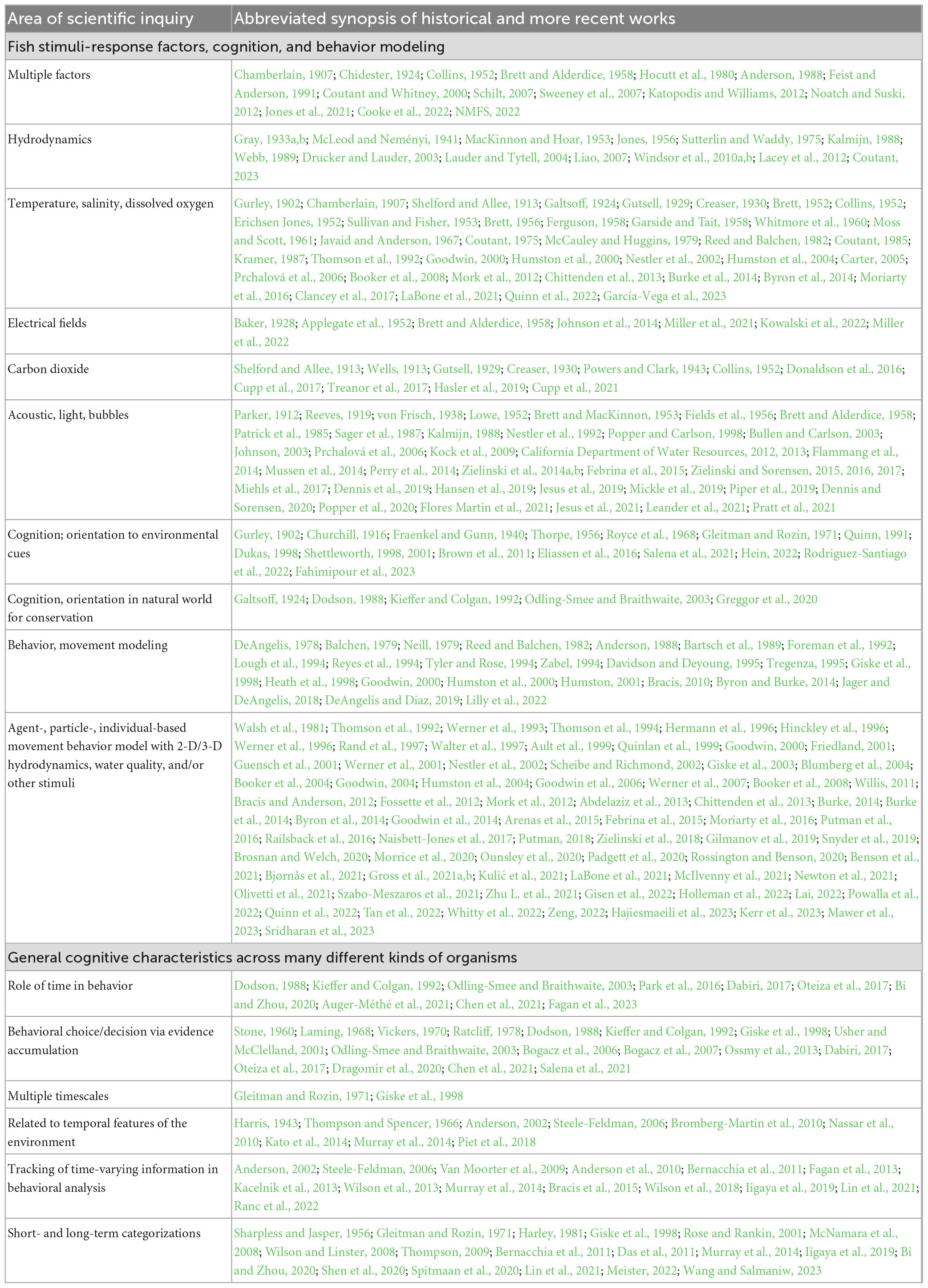
Table 1. Fish stimuli-response factors, cognition, behavior modeling, and general cognitive characteristics across many different kinds of organisms.
Here, we limit our focus to hydrodynamic stimuli. The study of fish and water flow has a rich history dating back about a century. Also dating back about a century yet somewhat separate from the hydrodynamic investigations is the study of fish cognition and how they orient to environmental cues, which have long been applied to understand their behavior in the natural world for conservation purposes (Table 1).
Ecological decision-making for conservation is inherently a forecasting problem (Werner et al., 2007; Dietze et al., 2018), and numerical modeling makes precise our underlying hypotheses (Dietze et al., 2018). Numerical fish behavior and movement modeling has been a powerful tool in conservation for more than 40 years (Table 1). Near-term ecological forecasting, specifically, focuses on meeting the needs of daily to decadal environmental decision-making under high uncertainty and adaptive management. Iterative near-term ecological forecasting involves rapidly testing hypotheses through comparison of quantitative predictions to new observational data under different scenarios, one of the strongest tests of scientific theory (Dietze et al., 2018). However, there is no such thing as a perfect forecast (Werner et al., 2007; Dietze et al., 2018). Key challenges remain.
The number of fish behaviors that need to be factored in order to reproduce movement and passage/entrainment patterns at river infrastructure increases concomitantly with environmental complexity (Goodwin et al., 2014). An important question for water operations management, therefore, is how different fish behaviors emerge, one at a time, from a multi-response repertoire to meet the momentary challenges of an individual. In other words, how does a specific fish-hydrodynamic response suited for a given environmental context emerge from an evolved repertoire of multiple behaviors that, together, facilitate the animal’s navigation through diverse, time-varying conditions such as flood and ebb tides (Dodson, 1988). We pursue three main lines of scientific inquiry in our study:
• what might the evolved repertoire of fish-hydrodynamic responses be for downstream-migrating fish in rivers;
• what degree of mathematical complexity is needed to reproduce and predict fish swim path patterns and observed passage/entrainment at infrastructure; and
• what level of numerical sophistication is required of river hydrodynamic modeling to inform a computationally-tractable management decision-support tool?
We cannot measure all internal and external factors in the natural world that may influence how a fish moves through an open river. However, sensory processing and cognitive decision-making is evident even in simple laboratory settings where an individual fish changes its behavior response over time to a stimulus that itself does not change (Haro et al., 1998; Enders et al., 2009a). In rivers, the same phenomena is observed near infrastructure (Goodwin et al., 2006, 2014). We piece together concepts, theory, and mathematics across multiple scientific fields as well as findings dating back in some cases nearly a century ago within the areas of organism sensory perception and cognitive decision-making, fish environmental and hydrodynamic response, and numerical behavior and environmental modeling (Table 1).
We start by, first, describing some general characteristics of cognition that apply to many organisms, not just fish. Then, second, we describe our tidal study system and data involving juvenile Pacific salmonids (hereafter salmon). Third, we tailor the general characteristics of animal cognition that we introduce in the next section to salmon navigating a tidal river junction in the context of water operations to understand and predict their movement and passage/entrainment.
2. Methods: general characteristics of animal cognition
The present era is one of rapidly developing knowledge about animal cognition (Greggor et al., 2020; Salena et al., 2021; Bialek, 2022; Hein, 2022; Petrucco et al., 2022; Triki et al., 2022; Wang and Salmaniw, 2023). At a fundamental level, we lack understanding of the complexities and context dependencies that underlie behavior changes in multisensory conditions (Bak-Coleman et al., 2013; Coombs et al., 2020). A critical part of interpreting changes in behavior is understanding the role of time (Table 1). One reason for our existing knowledge gaps is that invaluable laboratory experiments are also limited in the available degrees of freedom compared to the natural world (Salena et al., 2021), the latter of which involves continuous decisions with ever-changing options influenced by recent responses (Yoo et al., 2021). Fish may exhibit different behaviors in the field environment than in simpler settings (Dennis and Sorensen, 2020).
Note that for the purposes of our work herein that terminology can differ among scientific fields and, here, we take an expansive and inclusive view of the terms cognition and cognitive. By the terms cognition and cognitive we are referring generally to perception, attention, memory, learning, and the processes of perceptual decision-making that we can predict at the scale of a river. Also, we use the terms behavioral choice and decision interchangeably. We recognize that in our attempt to make our nomenclature understandable across a broad audience that we may deviate from more stringent terminology definitions in some of the scientific fields that we leverage in this work.
Our cognitive approach to mechanistic animal movement behavior modeling is not a study of brain architecture. We necessarily relegate many cognitive phenomena to parameterization that summarily represents subresolution dynamics that may seem crude if viewing our work from the perspective of other scientific fields that investigate neuroscience, neurobiology, and cognition at a finer scale. Here, we must encode cognitive phenomena more simply than what happens inside an animal’s brain in order for a model of movement behavior to operate at the scale of landscape and waterscape infrastructure in the open world for natural resources management.
2.1. Sensory experience influences stimulus perception and behavioral choice
The sensory experience of an individual strongly influences the perception of a stimulus (Akrami et al., 2018) and resulting behavioral choice (Table 1). Momentary stimuli are noisy, so animals constantly integrate sensory evidence over time and space to infer the state of their environment (Bahl and Engert, 2020; Dragomir et al., 2020). A relative difference between momentary and previously experienced stimuli influences the movement of even primitive organisms (Ikeda et al., 2020). In next section, we describe the first step in our modeling process for encoding how sensory experience influences the perception of a stimulus and resulting behavioral choice.
2.1.1. Stimulus: physical vs. perceived intensity
We first convert a stimulus physical (measured/modeled) value into a perceived intensity, Iφ, by applying a treatment analogous to the decibel scale for any stimuli variables whose quantities, φ, span orders of magnitude, such as gradients and other derivative values:
where φo is an arbitrary reference or baseline. The logarithm of a physical quantity, Iφ, at momentary time t often better represents an animal’s perception of intensity for a stimulus whose measured/modeled quantities span orders of magnitude (Fechner, 1860), e.g., sound. In our approach, physical stimulus quantities that do not span orders of magnitude remain unmodified from their measured/model value.
After this step, we refer to each stimulus i whose measured/modeled quantity is φ as its perceived intensity, Ii. Also, note that in limited places we use the terms quantity and intensity interchangeably in order to convey a few concepts herein.
A common feature of perception across taxa is the sensory system’s translation of a physical stimulus magnitude to a perceived quantity using proportional differencing (Akre and Johnsen, 2014). While our first step accounts for some psychophysical characteristics of perception, it does not account for an animal’s continuous sampling of the environment. In next section, we describe our approach for how continuous sensory sampling and experience over time influences an individual’s perception of a stimulus.
2.1.2. Stimulus: perceived change in intensity
Continuous sampling of a stimulus over time impacts how its perceived quantity may be registered by an animal. Each animal has its own unique sequence of preceding experiences, or history, so the momentary perception of a stimulus can be registered differently by separate individuals. Detecting the change in a stimulus using a proportional difference between two magnitudes allows an animal’s sensory system to cope with the enormous diversity of intensities experienced in the environment (Akre and Johnsen, 2014).
Note that in the first step, we converted stimuli to perceived intensities, yet the perceived change in intensity is also a perceptual characteristic. To keep our steps clear and nomenclature simple, hereafter, we refer to perceived intensity simply as intensity, Ii, so we can refer to the notion of a perceived change in perceived intensity more simply as the perceived change in intensity.
Our second step for encoding how sensory experience influences stimulus perception is to describe the perceived change in intensity, Ei, following an analogy to the just noticeable difference (jnd) concept of the Weber-Fechner law (Weber, 1846; Fechner, 1860). We compute Ei by comparing the momentary intensity, Ii, to recent past sensory experience in the form of a habituated (or acclimatized) level, Iai, at time t as:
Habituation is the foundation of selective attention that perceptually desensitizes an animal over time to static, common, irrelevant, or inconsequential stimuli. Habituation allows the individual to focus on the most salient signals in their environment at a given moment even amid high background noise (Rose and Rankin, 2001; McNamara et al., 2008; Rankin et al., 2009; Blumstein, 2016; Shen et al., 2020; Tafreshiha et al., 2021). Habituation is a form of plasticity, more specifically, a simple memory and learning process that is found across sensory systems and taxa, including fish (Dennis and Sorensen, 2020). Habituation is a building block of animal cognition and behavior (Harris, 1943; Konorski, 1948; Sharpless and Jasper, 1956; Thompson and Spencer, 1966; Peeke and Peeke, 1973; Rose and Rankin, 2001; McNamara et al., 2008; Das et al., 2011).
The jnd does not universally capture perceptual performance in every kind of task (Carriot et al., 2021). Our treatment of signal-to-background, or signal-to-noise jnd, Ei (t), is perhaps better described instead as a notable streaming differential (nsd) because animals update the ratio in Equation 2 perpetually, not just at a single decision moment in time that is often the basis for jnd evaluation. We use an exponentially weighted moving average (EWMA) to encode habituation although more sophisticated algorithms exist. Using an EWMA, the habituated intensity, Iai, updates as follows:
where Ii (t) is the momentary intensity of stimulus i at the individual’s xyz-position at time t, Iai (t) is the intensity of stimulus i to which the individual is habituated or, in other words, the background intensity. We assume the memory parameter mai is a non-changing coefficient within the range [0, 1] that determines how quickly the individual habituates and becomes desensitized to new intensities of the stimulus (Bush and Mosteller, 1955).
Sensory experience is the basis we use to encode a cognitively-inspired mechanistic account of the salmon’s changing environmental context for momentary decisions (Goodwin et al., 2006, 2014), which we describe as the third step in the next sections.
2.1.3. Context-based behavioral choice—with a single factor
Contrary to the notion that context is important in decision-making only for higher trophic level organisms, contextual awareness resulting in different responses to the same stimulus is a factor even in single cells (Kramer et al., 2022). An organism’s behavioral choice depends on the context of its momentary decision (Bak-Coleman et al., 2013; Coombs et al., 2020; Ikeda et al., 2020; Mann, 2020; Oram and Card, 2022). Sensory experience informs the decision context. Animal decisions are based on the simple notion of whether perceived conditions are better or worse than preceding experience (McNamara et al., 2013). In our approach, preceding experience is encoded through habituation, Iai.
In our approach, the previously experienced stimulus intensities provide the decision context when a single environmental factor is at play. We encode the momentary stimulus relative to the context of previous sensory experiences using the perceived change in intensity Ei.
Behavioral choice such as a change in movement orientation and speed within our approach is based on the notion of whether Ei exceeds a pertinent threshold, ki, where ki is a characteristic that must be determined in the analysis. Describing behavioral decisions using accumulated sensory evidence crossing a threshold (Bahl and Engert, 2020) is a common approach across a variety of organisms (Dragomir et al., 2020).
2.1.4. Context-based behavioral choice—with multiple factors
The natural world is composed of many factors, some known and many unknown, whose stimulus quantities are continuously integrated over time by an animal. Each stimulus competes for the individual’s selective attention. Determining the decision context of behavioral choice requires not only integrating intensities over time for multiple abiotic and biotic factors but also finding a common currency to combine the diverse sensory experiences toward a singular decision for the moment. Our approach to multiple factors is to use thresholds, ki, for each factor or stimulus i. We combine the sensory experiences across multiple factors by converting threshold exceedances into Boolean values [0 or 1], which we can use as a common currency to combine diverse sensory experiences to inform momentary choice.
An animal’s movement strategy in natural settings may consist of a large repertoire of behavior responses. A stimulus operates on a spectrum, so the concept of a threshold helps in interpreting at what point does the factor warrant attention relative to competing factors. When the animal experiences a diverse array of environmental stimuli and conditions, behaviors within a repertoire may take varying precedence in different phases of a movement sequence (Sogard and Olla, 1993; New et al., 2001).
In our approach, an individual perpetually updates and compares their nsd values at time t, Ei (t), to corresponding thresholds, ki, for each stimulus i. When Ei (t) crosses ki we assume the neural activity, aB (t), in the animal’s brain increases their propensity or motivation – mathematically, what we call accumulated evidence, eB (t) – to respond with behavior B (t) {r} using one of the available responses, r, within the evolved repertoire, r = {1, 2, 3, …}. Put simply, when Ei (t) crosses ki we assume the corresponding stimulus i warrants attention, even if no movement response is yet required; stimulus i begins to climb in the hierarchy of competing other stimuli. Mathematically, when the threshold is crossed then the Boolean measure switches from 0 to 1. When the Boolean measure is 1, then activity aB (t) takes on a value within the range [0.0 < aB ≤ 1.0] that does not change with time and whose value is determined in the analysis. The constant aB is based on a subjective assessment of the response’s value to the animal relative to the other behaviors in the larger repertoire. Activity aB (t) is zero whenever the threshold is not crossed.
The evidence, eB, supporting each behavior B accumulates based on inputs aB (t) through a cognitive algorithm and results in the selection of a singular movement orientation and speed response for the duration of time increment △t. The temporal integration of evidence supporting different choice options — each behavior response B — is a computational process generally thought to underlie decision-making (Ossmy et al., 2013) and accurately describes paradigms with multiple sensory modalities across various organisms (Dragomir et al., 2020). The exact currency of evidence that is accumulated (e.g., sensory versus behavioral output) is an active area of neurophysiological study (Dragomir et al., 2020).
In our present approach, following the sensory integration paradigm, we use the Mutual Inhibition Model or Leaky Competing Accumulator model (Usher and McClelland, 2001) to temporally accumulate perceived evidence and select the behavior B. To decide behavior transitions, the sensory evidence accumulators, eB, integrate the activity, aB, supporting each behavior B as:
or as a complete equation in discrete form:
where eB (t = 0) = 0. The behavior B (t) {r} implemented at time t is the response r associated with the greatest accumulator value eB at the beginning of increment △t. eB is a leaky integrator that accumulates evidence from a drifting input with mean activity aB (Bogacz et al., 2006). Activity aB corresponds to a general, inherent urgency to respond to the stimulus with a particular behavior B (Schurger et al., 2012). Each behavior B is associated with an activity aB that causes it to be implemented in the face of other available responses. An individual executes behavior B when the activity aB supporting it accumulates over time in the form of accumulator eB from Equation 4 or 5 and overtakes the accumulators, e, of the other available behaviors that could otherwise be implemented.
λ is the exponential decay rate of activity aB where the leak term −λeB causes eB to decay to zero in the absence of inputs aB. When λ > 0, the net effect is decay toward zero that produces stability in the activation whereas for λ < 0 the activation tends to self-amplify and is not stable (Schurger et al., 2012). The accumulators eB mutually inhibit each other through a connection weight, η, where S is the number of accumulators eB. The variable having uppercase W may be thought of as random fluctuations in the signal, intrinsic accumulator noise, or unmodeled inputs and can be represented as independent, identically distributed Wiener processes with unit variance (McMillen and Holmes, 2006).
In the discrete form, ζB is Gaussian noise sampled from a standard normal distribution N(0,1) with zero mean and variance σ2 = 1, c is a noise-scaling factor, and △t is the discrete time increment of the simulation (Usher and McClelland, 2001; Bogacz et al., 2007; Schurger et al., 2012; Tsetsos et al., 2012). λ and η are all assumed to be nonnegative. The activity scale can be chosen so that zero represents baseline activity in the absence of inputs, hence integration starts from eB (t = 0) = 0 (Bogacz et al., 2006). The major simplification of the model here compared to that of Usher and McClelland (2001) is the removal of nonlinearities (Bogacz et al., 2006). eB accumulation rates depend linearly on their present values. To account for the fact that neural firing rates in the brain are never negative, Usher and McClelland assumed that eB is transformed via a threshold-linear activation function:
or more simply:
Usher and McClelland (2001) propose that a multi-decision process can be modeled by a direct extension of the Mutual Inhibition Model in which each eB inhibits and receives inhibition from all other eB. This implements a max-versus-average procedure where evidence favoring the most supported alternative is compared with the average of the evidence in support of all other alternatives (Bogacz et al., 2006). Usher and McClelland (2001) show the approach performs best among several alternative models. Behavior selection is an ongoing decision process, perpetual in time, and cross-inhibition robustly improves its efficiency by reducing the frequency of costly transitions (Marshall et al., 2015).
2.1.5. Multiplex signal disentanglement via multi-timescale perceptions
Animals must be responsive to information that changes locally as well as broader environmental shifts. Both local short-term and broader longer-term information inform the next behavioral choice through shifts in the decision context. Animals sample their landscape from a single position per unit time. Discerning whether a perceived change stems from updated positioning or broader environmental shifts is straightforward when the stimuli are relatively steady (unchanging with time) as the animal samples the space. When the landscape itself changes with time at nearly the same temporal scale that the animal samples its surroundings, disentangling self-guided and external factor contributions to perceived shifts in environmental context is less straightforward.
Distinguishing local versus larger-scale change is relatively straightforward from a Eulerian (outside human observer) point-of-view compared to the Lagrangian perspective of an individual limited in sensory range and to a single sample per unit time. Multiple perceptions operating at different timescales can disentangle environmental factors occurring at more than one spatiotemporal scale using only a single sample per unit time. In our approach, the animal serially samples its local surroundings once per unit time but can generate one or more parallel images of the environment at different spatiotemporal scales by tracking serial samples with multiple concurrent habituations (memories). Multiple memories, or habituations, encode information that the animal can later use to discern perceived environmental shifts at different spatiotemporal scales.
The notion of multiple timescales is not new (Table 1). Existing theory already suggests that animals integrate fluctuating sensory cues over multiple timescales relevant to the temporal features of their environment. Multiple integrations or memory timescales, such as in habituation, are frequently categorized as short- and long-term (Table 1). Shorter forms may be as fast as hundreds of milliseconds (Szyszka et al., 2012) and longer forms as slow as days (Sharpless and Jasper, 1956).
In behavioral analyses, multiple memory streams are a powerful means to account for the tracking of time-varying information (Table 1). While questions remain regarding the specific relationship between short- and long-term memory processes (McGaugh, 2000), it is generally recognized that slower-updating (longer-term) and faster-updating (shorter-term) memories can coexist (Bernacchia et al., 2011; Murray et al., 2014; Iigaya et al., 2019).
We expand Equation 3 to now include two timescales of integration for cognitively tracking long-term (slower) and short-term (faster) habituations to a stimulus i, denoted as and , respectively:
with the memory values bound within the range of [0, 1], where superscript slow indicates the quantity updates at a slower rate since a larger m value more heavily weighs the past. We treat timescale integration (memory) parameters and as fixed but, in reality, they could themselves be context-dependent.
The dual timescale approach is a simple computational method for encapsulating the notion of multiple timescales that, in reality, are complex neural phenomena (Thompson, 2009; Bi and Zhou, 2020; Shen et al., 2020; Spitmaan et al., 2020). Two timescales of integration allow an individual with serial sampling of the landscape or waterscape to disentangle dual overlapping contexts occurring simultaneously; for example, detecting a spatial gradient amid rapid time-varying changes while immersed in a media that itself is moving, such as water.
The material discussed thus far does not stem primarily from fish or the aquatic realm and, therefore, is likely applicable to movement ecology questions in terrestrial, avian, and subterranean environments. Next, we describe the details of our tidal river salmon study before revisiting the general cognition characteristics tailored specifically to our analysis. Note that, at field scale, it is not yet possible to disentangle the relative contributions of all the potential abiotic and biotic factors that might be responsible for observed salmon movement. Therefore, our notion of cognition likely inadvertently encapsulates other factors that influence a fish’s hydrodynamic response such as physiological condition, internal or bioenergetic state, change in risk disposition, etc.
3. Tidal river salmon movement behavior
In this section, we introduce the diverse and time-varying river conditions of our tidal system and the data available. Then, we describe the details of our cognitive approach to mechanistic behavior modeling tailored specifically to interpreting and predicting salmon movement and passage/entrainment.
3.1. California’s Bay-Delta
The Sacramento-San Joaquin Rivers Delta that, together with San Francisco Bay, is often referred to as California’s Bay-Delta supplies drinking water to 27 million people, fuels a $32 billion agricultural industry, and is habitat for more than 750 animal and plant species (California Department of Water Resources, 2022). The tidally influenced Sacramento River bifurcation at Georgiana Slough in Walnut Grove (Figures 1, 2) is part of the managed water supply system. A management goal at the bifurcation is to direct juvenile salmon so their movement continues downriver using the Sacramento River, which leads more directly to the Pacific Ocean where these fish mature to adults. Salmon migrating through the alternate route, Georgiana Slough, take a longer path to the ocean that may also be associated with reduced survival probability (Perry et al., 2018).
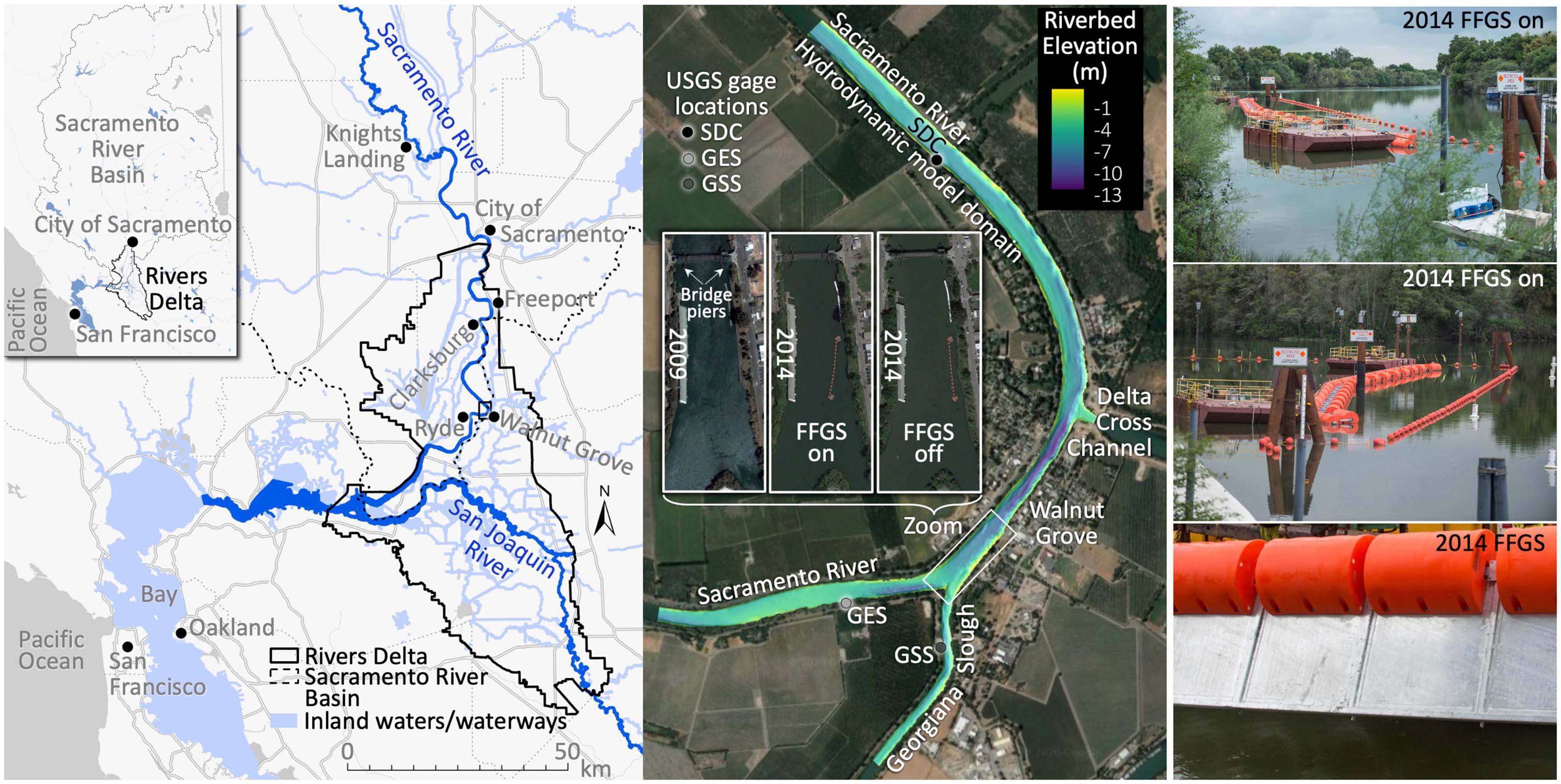
Figure 1. The Sacramento River reach between the Delta Cross Channel and Georgiana Slough in Walnut Grove, California used for our analysis is located between river miles 26 and 28. The reach is located between the cities of Sacramento and San Francisco within the Sacramento-San Joaquin Rivers Delta (left panels). The floating fish guidance structure or surface guidance boom (FFGS) is deployed only during year 2014 (middle and right panels). FFGS field photo credit: California Department of Water Resources. Bathymetry data: U.S. Geological Survey, California Water Science Center. Map data: Google, Maxar Technologies, U.S. Geological Survey, USDA Farm Service Agency.
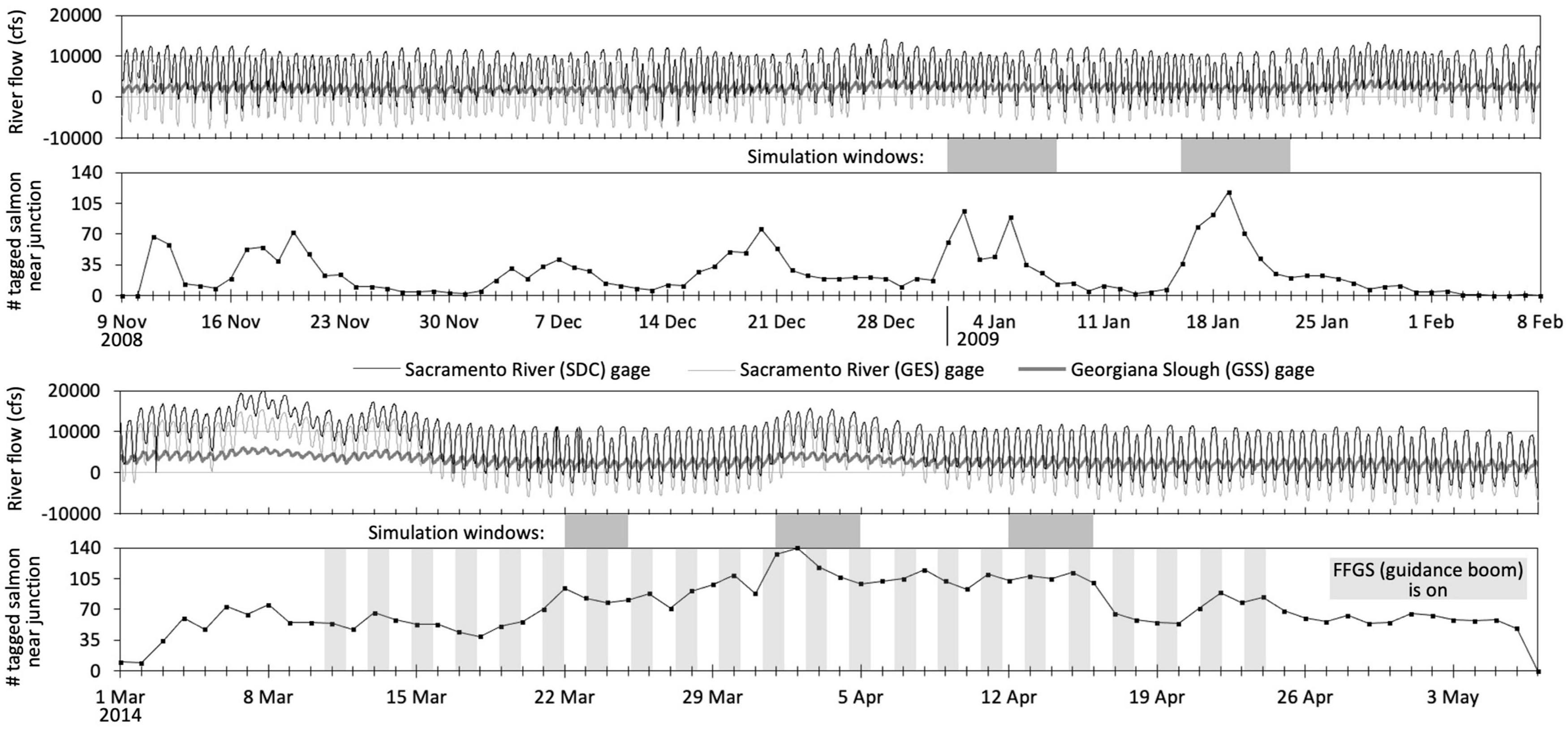
Figure 2. The tidally influenced flow of the Sacramento River bifurcation at Georgiana Slough during the 2008–2009 and 2014 studies. Negative river flows move upriver away from the ocean. The graph of tagged salmon counts from acoustic-tag telemetry (Romine et al., 2013, 2017; California Department of Water Resources, 2016) depicts the number of unique individuals observed at the junction with at least four consecutive detections within a day. Our analysis timeframes, or simulation windows (darker grayed blocks), correspond to the dates with the largest number of tagged salmon observed near the junction. FFGS is the floating fish guidance structure or surface guidance boom (Figure 1). Flow gage locations (SDC, GES, GSS) shown in Figure 1. cfs is cubic feet per second. Gage flow data from the U.S. Geological Survey (2020).
We use salmon acoustic-tag telemetry and hydrodynamic data from the Sacramento River between the Delta Cross Channel and Georgiana Slough to better understand and predict the stimuli-response behaviors of the fish that result in their ultimate fate (passage, entrainment) and movement patterns. We use data within five analysis or simulation windows (Figure 2 and Table 2) from two field study seasons. We use year 2009 data (two windows: 1–7 and 16–22 January) to fully build and parameterize the fish behavior model. Later, we then apply the model without any modification to year 2014 flow conditions that include a novel surface guidance boom (three windows: 22–24 March, 1–4 and 12–15 April) to assess predictive performance on out-of-sample data.

Table 2. Tagged salmon data in analysis.
3.1.1. Salmon field data details
The fish used in the 2008–2009 and 2014 studies are juvenile late fall-run Chinook salmon obtained from the Coleman National Fish Hatchery operated by the US Fish and Wildlife Service. The mean fork length of the 3,551 tagged salmon in 2008–2009 is 149.9 mm (Romine et al., 2013), and in year 2014 the average is 157 mm with a range of 109 − 213 mm across the 5,461 individuals with acoustic transmitters (California Department of Water Resources, 2016; Romine et al., 2017).
Of the 3,551 tagged salmon in 2008–2009, 1,772 (49.9%) are released downriver of the Georgiana Slough junction with the Sacramento River; specifically, 690 downriver in Ryde in the Sacramento River (river mile 24) and 1,082 in Georgiana Slough (Figure 1). All other tagged salmon are released upriver approximately 53 km (33 miles) in the City of Sacramento at the Tower Bridge (river mile 59). In year 2014, 826 of the 5,461 tagged salmon (15.1%) are released in Georgiana Slough approximately 5 km (3 miles) downriver of the junction with the Sacramento River, and all others are released upriver in the City of Sacramento.
We filter out the following tag detections:
• known predator tags as well as tagged salmon that at any point during their observation are assigned a predator probability greater than or equal to 0.85 in the range [0, 1] based on previous work by Romine et al. (2014), where 1.0 suggests a predator and 0.0 a salmon. Some tagged individuals are released as known predators, and any fish released dead is classified as a predator. All fish released into Georgiana Slough during the 2008–2009 study and later observed near the junction are assumed to be predators (Romine et al., 2014). One predator during the 2008–2009 study ate five tagged salmon, and these tags are classified as predator;
• spatial positioning errors greater than 10 m. Georgiana Slough is only about 45m wide near the junction;
• consecutive tag detections less than 2s apart in order to sample the telemetry data as analogous as possible to the time step of modeled salmon described later;
• consecutive tag detections that would require a speed over ground greater than 2.5 m s−1, a threshold cutoff slightly stricter than would be calculated (2.65 m s−1) by combining the maximum water speed during our simulation windows of about 0.65 m s−1 (from the hydrodynamic modeling described later) and a generic 200−mm fish with a short-duration burst swim speed of 2 m s−1 or 10 body lengths per second (Beamish, 1978).
3.1.2. Salmon movement patterns
Tagged salmon in the Sacramento River exhibit several distinct movement modes. We classify every tagged salmon path in the Sacramento River reach between the Delta Cross Channel and Georgiana Slough during our simulation windows using visual inspection according to the following predominant patterns (Figure 3):
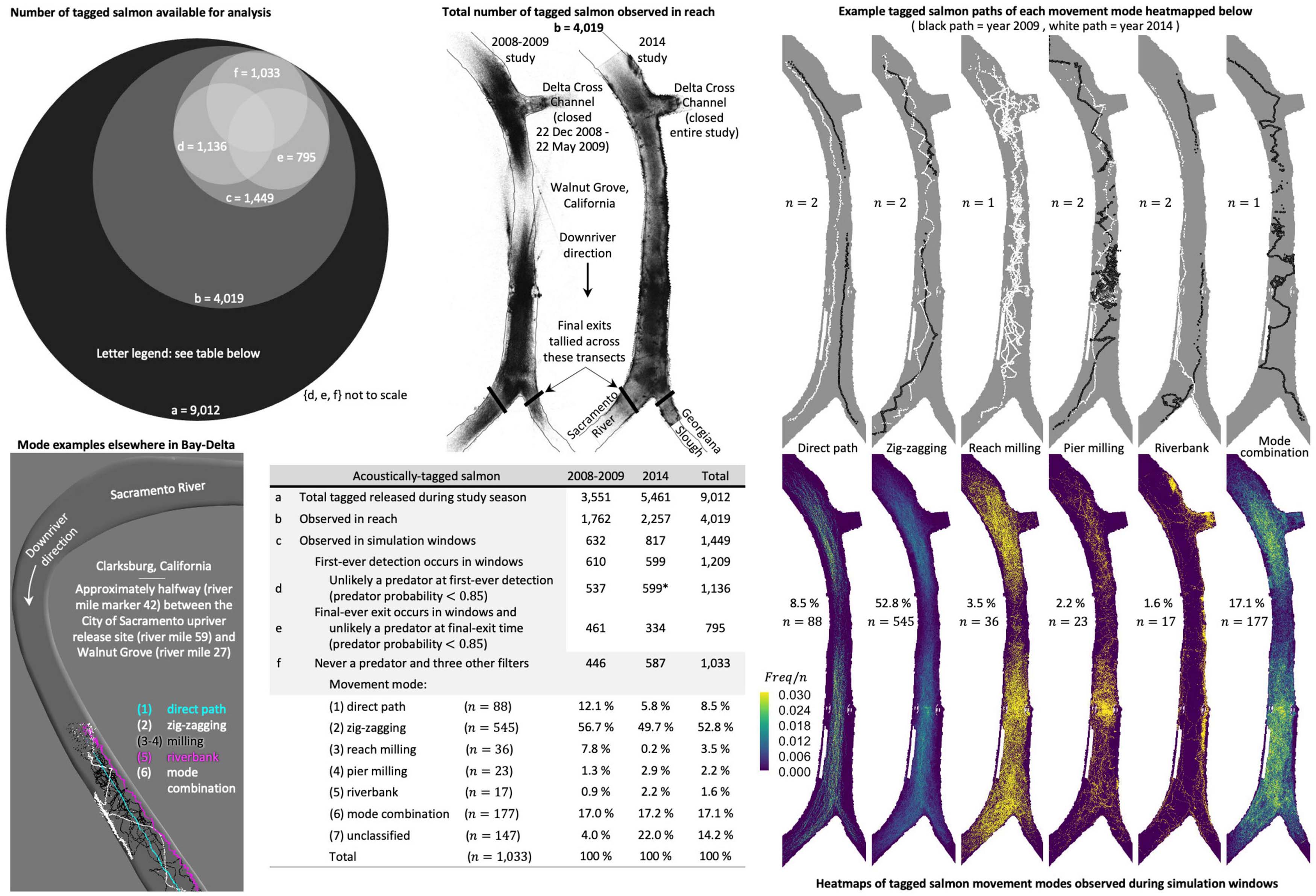
Figure 3. Available acoustic-tag telemetry data (upper-left, upper-middle, table in lower-middle), movement mode heatmaps (lower-right), example tagged salmon swim paths of each mode (upper-right), and the modes exhibited elsewhere in the Bay-Delta (lower-left). Tabulated are the (a) total tagged salmon released during the 2008-2009 and 2014 studies, (b) the number detected in the Sacramento River reach between the Delta Cross Channel and Georgiana Slough, (c) within our simulation windows, and (d–f) unlikely a predator at moments the data is used in our analysis. Heatmaps are computed after removing suspected predators, tag detections with spatial error greater than 10m, and consecutive positions either less than 2s apart or require a speed over ground in excess of 2.5 m s−1 (f). n equals the total tagged salmon in the movement mode category. Example constituent paths of each movement mode are plotted above the respective heatmap. Movement modes (1)–(6) are observed elsewhere in the Bay-Delta (gray inset) in a supplemental 2014 hydrophone array (California Department of Water Resources, 2016). We assume all tagged fish detected for the first time ever during our 2014 simulation windows are salmon (*) whereas year 2009 predator probabilities are formatted differently and allow us to identify and remove suspected predators at a tag’s initial detection (d). We use transects immediately downriver of the junction to determine tagged salmon final exits downriver (e) (Table 2) also referred to as passage or entrainment. The Delta Cross Channel is closed during our simulation windows (Figure 2).
| (1) direct path | — | no milling or zig-zag movements greater than 1/3 of the river’s width; |
| (2) zig-zagging | — | at least one cross-stream excursion sustained for more than 1/3 of the river’s width. Path can include brief, intermittent milling and/or shoreline movement but no appreciable double-backing within the reach between the Delta Cross Channel and Georgiana Slough; |
| (3) reach milling | — | milling predominant throughout the reach between the Delta Cross Channel and Georgiana Slough; |
| (4) pier milling | — | distinct milling near the Walnut Grove Bridge piers; |
| (5) riverbank | — | movement and milling predominantly near the riverbank; |
| (6) mode combination |
— | combination of two or more of (1) direct path, (2) zig-zagging, (3–4) milling, and (5) riverbank; |
| (7) unclassified | — | mode not readily classifiable, typically because the swim path has few detections, spatial gaps in key areas, a massive number of detections in a small area that persist for a while, or does not span the majority of the reach between the Delta Cross Channel and Georgiana Slough. Tag detections in the upriver portion of the reach during 2014 have, at times, more gaps and imperfections than 2008–2009 data, resulting in more contributions to this class. |
Tagged fish released downriver of the junction may not swim upriver into the Sacramento River as far as the Delta Cross Channel during our simulation windows and, thus, often contribute to the unclassified count. Our classifications are analogous to those developed independently in prior work by the U.S. Geological Survey in a turning point analysis of the tagged fish; see page 3–215 of California Department of Water Resources (2016).
Heatmaps of the movement modes (Figure 3) illustrate the pattern of all mode-classified tagged salmon. A heatmap is the number (frequency, Freq) of unique individuals visiting a 1−m square grid cell filling the domain, normalized by the total tagged salmon in the movement mode category (n in Figure 3). Only detected tag positions are heatmapped, that is, paths are not implied from the position sequence.
Zig-zagging is, by far, the predominant movement mode in the Sacramento River reach between the Delta Cross Channel and Georgiana Slough in Walnut Grove. Salmon zig-zagging is not unique, however, to the Walnut Grove reach in the Bay-Delta. Zig-zagging and other movement modes are also observed upriver in Clarksburg (Dinehart and Burau, 2005) about halfway between the City of Sacramento release site and Walnut Grove (Figures 1, 3). A single salmon exhibiting more than one movement mode in a short period of time can be observed in two examples within Figure 3. First, just upriver of Georgiana Slough (Figure 3, upper right) a salmon alternates between zig-zagging, pier milling, and the riverbank movement modes. Second, upriver, a salmon can be seen zig-zagging, transitioning to a riverbank mode, and then back again to zig-zagging (Figure 3 inset of Clarksburg, California—white fish trajectory).
Habitat refuge, vision (Leander et al., 2021; Müller et al., 2021), and explicit response to spatial structure (Braithwaite and Burt de Perera, 2006; Miles et al., 2023) may play modulating roles in salmon movement. Also, behavioral variation among individuals of the same species is common (Bolnick et al., 2002; Bierbach et al., 2017; Cresci et al., 2018; Campos-Candela et al., 2019; Harrison et al., 2019; Honegger et al., 2020; Bailey et al., 2021; Daniels and Kemp, 2022) as it has distinct survival value (Humphries and Driver, 1970). We do not attempt to disaggregate or prioritize the relative contribution of all internal and external factors. Here, we focus on understanding the predominant zig-zagging swim path pattern and how it with smaller proportions of other movement modes might be hydrodynamically mediated.
3.1.3. Protean movement decisions and optimality
Movement is a behavior that operates within a hierarchy of needs, where predation is a constant threat for prey species. Predation complicates the analyses of behavioral choice in real-world environments because rote responses easily discerned by an outside observer may also be predictable from a predator’s perspective. Protean movement in which a prey’s path changes frequently, helps evade predators (Humphries and Driver, 1970; Godin, 1997; Richardson et al., 2018). Selective evolutionary pressure suggests that predators exploit repeated fixed patterns of prey (Humphries and Driver, 1970; Domenici et al., 2008), although perhaps not universally (Szopa-Comley and Ioannou, 2022). Peculiarities in observed movement that appear sub-optimal from an outside observer’s perspective may be anti-predatory characteristics whereby optimality is realized at the much larger scale of species persistence. It is increasingly recognized that perceptual decision-making at the individual level in natural settings with multiple alternatives is suboptimal (Yeon and Rahnev, 2020).
3.1.4. Zig-zagging
Salmon persist in the “predator-prey arms race” (Humphries and Driver, 1970; Kelley and Magurran, 2006) of California’s Bay-Delta, which suggests that they may have an anti-predatory characteristic to their downriver navigation strategy. When visual cues are limited underwater, zig-zagging keeps a prey’s average position within the river channel unpredictable from the perspective of an immersed predator (Humphries and Driver, 1970). Prey zig-zagging is a protean movement pattern often thought to occur in small arenas where it lowers a predator’s targeting accuracy (Furuichi, 2002; Jones et al., 2011; Richardson et al., 2018; Gazzola et al., 2021), however, juvenile salmon zig-zag also in the large spatial domains of dammed reservoirs; see telemetry data references in the supporting information appendix of Goodwin et al. (2014).
3.2. Fish movement behavior and hydrodynamics
3.2.1. Determining fish movement behavior starting with particles and particle tracking
To understand the relationship between salmon movement and hydrodynamics, we must first understand how the river environment itself is described and the assumptions that are involved. Water flow is described by the Navier–Stokes equations but conceptualizing a river’s advective contribution to a fish’s displacement in space (x, y, z Cartesian coordinate positions) is not trivial, especially when hydrodynamics changes with time and location.
The movement of an ‘active’ particle that is moving under its own motivation contributes volitionally to its spatial position (Patlak, 1953; Siniff and Jessen, 1969; Kareiva and Shigesada, 1983), e.g., a fish locating within a river via swimming. In water, the change in spatial position of a swimming fish can be described mathematically between time step t and t + 1 as follows:
where x, y, and z are the individual’s spatial position (m), u, v, and w are the water velocity vectors (m s–1), uvolitional, vvolitional, and wvolitional are the volitional contribution from swimming (m s–1), and △t is the time step increment (s).
A fish that does nothing (no volitional movement) is transported by the surrounding water flow while, in contrast, an individual with an unbiased, uncorrelated random walk within a non-advective environment such as a static lake typically exhibits some form of diffusion in its location over time. In an advective environment, such as a river or estuary, the diffusive property of a random walk can be appreciably altered by the advection.
In general terms, the movement path of a volitional random walk is stretched in the direction of the water flowline and the degree to which this happens depends on the strength and complexity of flow (river hydrodynamics). A “passive” particle that is neutrally buoyant and massless will follow the water flowline and provides a means to conceptualize and mathematically determine the contribution of physical water flow to an entity’s movement (displacement) in a river. The movement of a simulated passive particle, however, depends inherently on the accuracy and spatiotemporal resolution of the available water flow data (Déjeans et al., 2022). Therefore, determining an entity’s volitional movement behavior (which equals the measured total movement minus what a passive particle would do) depends also on the accuracy and spatiotemporal resolution of the available water flow data. As there are numerous methods for describing hydrodynamics within a river, with different tradeoffs, we provide a brief synopsis before describing the stimuli that we use in our analysis.
3.2.2. Describing river hydrodynamics via numerical modeling and measurement
Fish in rivers experience turbulence that may be thought of as water flow composed of a wide continuum of eddy sizes where larger eddies spawn smaller ones, passing on kinetic energy, down to the scale where viscous forces dampen or dissipate the phenomenon (Tritico and Cotel, 2010; Rodi, 2017; Crowley et al., 2022). In rivers, where width is often much larger than depth, the eddy size continuum has two ranges. Smaller-scale motions are fairly random whereas larger fluctuations interact with the mean flow and often have some order and correlated pattern (coherent structures). In each range, the largest eddies that contain the most energy are limited by the size of the river dimension (Rodi, 2017).
The straightforward approach to simulating the Navier–Stokes equations in order to describe river water flow dynamics is direct numerical simulation or DNS (Orszag and Patterson, 1972; Moin and Mahesh, 1998). DNS does not require any model assumptions and accounts for fluid phenomena across the many spatiotemporal scales relevant to fish, down to the smallest dissipation scale. DNS simulation of river flow, however, is impractical with present-day computing. For instance, a relatively low energy water domain just 0.1 m deep moving slowly at 0.1 m s−1 requires approximately one billion computational mesh points (Keylock et al., 2005), and the required grid size grows quickly with increasing flow complexity and energy. All other approaches to the Navier–Stokes equations involve approximating their full complexity (Keylock et al., 2012).
There are numerous approaches to modeling river hydrodynamics, and every method involves tradeoffs (Lane et al., 1999; Keylock et al., 2012; Rodi, 2017; Robinson et al., 2019; Brunner et al., 2020). A simple way to gain information about the time-varying nature of hydrodynamics is an unsteady Reynolds averaged Navier–Stokes (RANS) approach where motions and variations in the mean flow field account for eddy-shedding at scales greater than the integral timescale (Keylock et al., 2005). RANS renders a smoothed, or averaged, version of the water flow field and, presently, is a common workhorse of river hydrodynamic modeling.
An intermediate approach between DNS and RANS (Rodi, 2017) is large eddy simulation or LES (Smagorinsky, 1963; Bedford and Babajimopoulos, 1980; Mahesh et al., 2004; Khosronejad et al., 2016, 2020; Le et al., 2019; Flora, 2021; Flora and Khosronejad, 2021, 2022). LES resolves eddy phenomena larger than a given filter scale, not just above the integral timescale as in unsteady RANS (Keylock et al., 2005). LES resolves eddies down to the mesh element size, and smaller scale phenomena are approximated with a subgrid-scale model (Keylock et al., 2012; Rodi, 2017). LES is more sensitive to the treatment of the river’s boundary conditions than RANS (Rodi, 2017), which is one reason why hybrid LES-RANS approaches have emerged such as detached eddy simulation or DES (Spalart and Allmaras, 1992; Spalart et al., 1997; Constantinescu et al., 2011a; Keylock et al., 2012). LES and DES require more nodes and are more computationally expensive than RANS. The river flow field described by LES or DES is closer to what a fish experiences (Figure 4), but the temporal sequence of LES or DES outputs can be challenging to synchronize with a specific calendar date-time. In other words, it is not straightforward to determine whether an ephemeral eddy feature of interest from LES or DES occurred before, during, or after a measured fish passed through that part of the river.
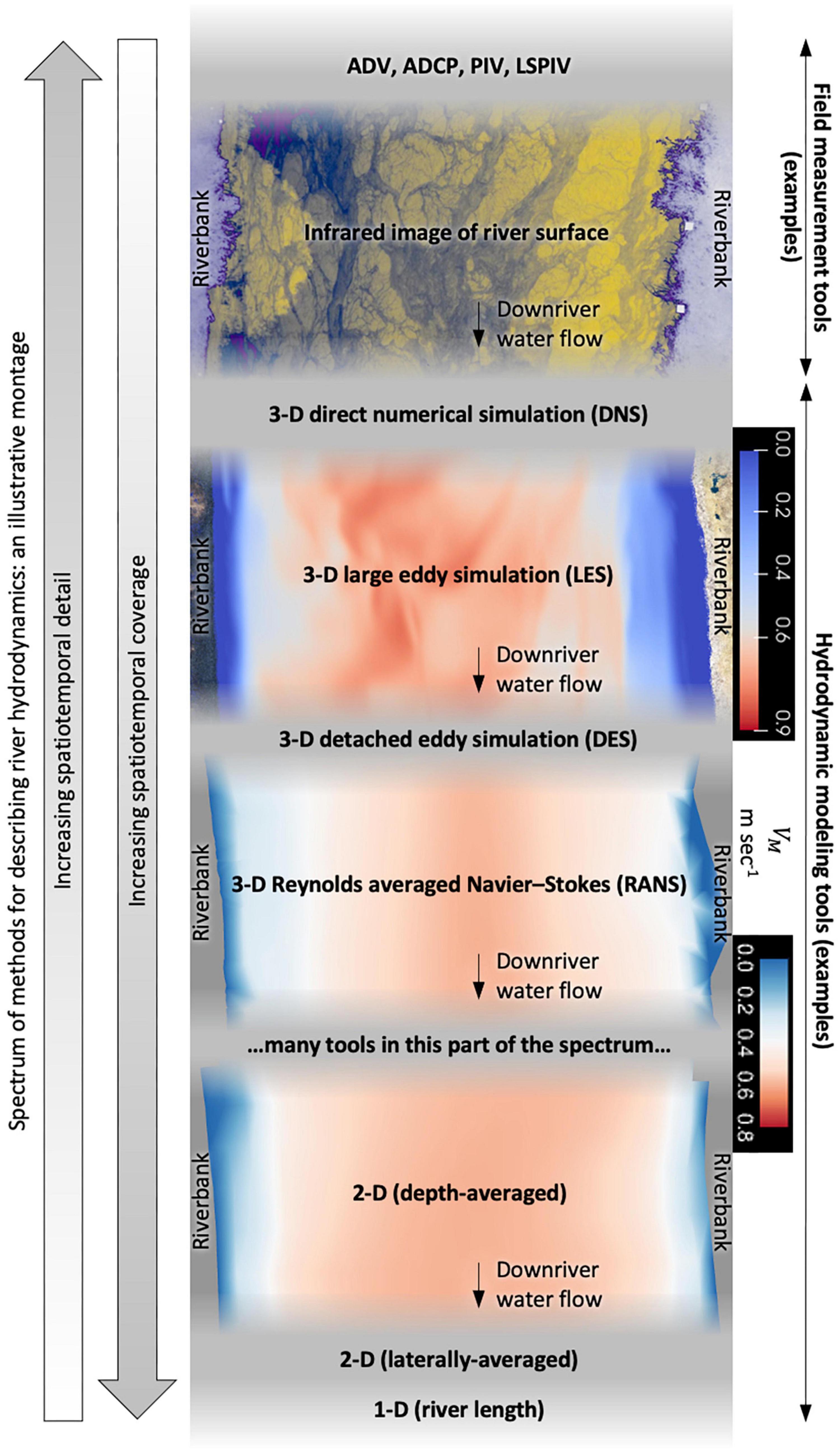
Figure 4. Rivers have more hydrodynamic heterogeneity than can be readily captured by any single measurement device or computational model. Here, we use a conceptual montage to illustrate some of the general tradeoffs in spatiotemporal detail vs coverage associated with different approaches to measuring/modeling river hydrodynamics. The fidelity of hydrodynamic information available influences the factors attributed to 3-D/2-D fish movement trajectories and behavior. Water flow heterogeneity within a river at the surface can be measured in detail via an infrared camera that reflects underlying hydrodynamic phenomena, illustrated here near Sacramento River mile 34 in Sutter Slough (courtesy of Seth Schweitzer; Schweitzer and Cowen (2021)). Water flow heterogeneity can also be modeled in great 3-D detail throughout the river column using LES, illustrated here near Sacramento River mile 89.5 (courtesy of Kevin Flora; Flora and Khosronejad (2022)). Describing river hydrodynamics with infrared quantitative image velocimetry (IR-QIV, Schweitzer and Cowen (2021)) or LES (Khosronejad et al., 2016; Flora and Khosronejad, 2022) provides more spatiotemporal detail than is possible using the 3-D RANS or 2-D depth-averaged methods in our study. In 3-D LES and RANS modeling, the hydrodynamic variable values are provided explicitly at multiple depths whereas 2-D depth-averaged models provide only a single value for each horizontal (xy-plane) location. However, RANS and even 2-D models render more spatial heterogeneity than other, courser forms of hydrodynamic modeling. The 3-D RANS and 2-D depth-averaged illustrations of the river flow field here are of similar conditions in the Sacramento River near mile 27 between the Delta Cross Channel and Georgiana Slough upriver of the bridge piers. ADV is an acoustic Doppler velocimeter; ADCP is an acoustic current profiler now commonly referred to as an acoustic Doppler current profiler; PIV is particle image velocimetry; LSPIV is large-scale particle image velocimetry.
For most rivers, water depth is shallow relative to width so the vertical acceleration is negligible compared to gravitational acceleration (Lai, 2010). In shallow water situations, the Navier–Stokes equations can be vertically averaged (Rodi, 2017). Two-dimensional, depth-averaged modeling of the Navier–Stokes equations provides the next level of accuracy when 3-D is not required, and the approach is practical for many river applications with a more typical desktop computer. 2-D depth-averaged approaches require considerably less computational resources. Numerous modeling approaches occupy the spectrum between RANS and simpler 2-D and 1-D methods, often covering much larger spatial domains (Zhang et al., 2016; Savant et al., 2018; Robinson et al., 2019; Brunner et al., 2020).
The selection of hydrodynamic model involves accounting for whether the additional required resources are balanced by the needed improvements in predictive ability and utility (Lane et al., 1999; Lai, 2010; Robinson et al., 2019; Brunner et al., 2020). The field of hydrodynamic modeling continues to rapidly evolve, and emerging methods such as physics-informed neural networks (Karniadakis et al., 2021; Kochkov et al., 2021) and other forms of machine learning (Margenberg et al., 2022; Vinuesa and Brunton, 2022; Zhang et al., 2022) are expanding the viable approaches.
Generally, one can measure river hydrodynamics at finer spatiotemporal scales than modeling can render them, but at the expense of spatial coverage (Figure 4). Acoustic Doppler velocimeters (ADVs) measure water velocity many times a second at a single point. Acoustic current profilers now commonly referred to as acoustic Doppler current profilers or ADCPs (Muste et al., 2004; Dinehart and Burau, 2005) measure the flow field many times a second at multiple distance intervals from the aimed instrument and are often able to span much of a river’s width or depth. Particle image velocimetry or PIV (Soo et al., 1959; Adrian, 2005; Tritico et al., 2007) and large-scale particle image velocimetry or LSPIV (Fujita, 1997; Fujita et al., 1998; Muste et al., 2008) measure instantaneous velocities in a 2-D plane using tracers present in the flow. Infrared quantitative image velocimetry or IR-QIV (Schweitzer and Cowen, 2021) measures instantaneous velocities at the 2-D water surface without tracers or illumination and can be used both day and night. A continuing active area of research is developing methods to estimate 3-D subsurface hydrodynamics from river-wide measurements at the water surface (Johnson and Cowen, 2016, 2017a,b,2020). Increasing the spatial coverage of river measurements can be accomplished by deploying multiple instruments or, in some cases, moving the instruments to capture different flow field regions.
To date, no measurement or modeling technique can accurately describe hydrodynamics down to the finest scale that fish detect throughout a 3-D river reach. We use field measurements of the river’s flow and bathymetry to build and validate a RANS model of the time-varying 3-D hydrodynamics for year 2009 (Lai, 2000; Lai et al., 2003, 2017). Later, for year 2014, we use a 2-D depth-averaged model (Lai, 2010). For both models, we output river hydrodynamics at 3-min intervals because the water flow field at the junction of the Sacramento River and Georgiana Slough can change noticeably within a few minutes and frequently reverses direction (Figure 2). Our 3-D RANS and 2-D depth-averaged model mesh domains (Figure 1, middle plot) are approximately 550,000 and 50,000 vertices, respectively, for each 3-min time increment.
3.2.3. Eulerian-Lagrangian-agent method (ELAM)
River hydrodynamics output from our 3-D RANS and 2-D depth-averaged modeling determines the river’s advective contribution (u, v, and w water velocity vectors) to the fish’s spatial displacement during an increment of time (Equation 10). To compute the fish’s volitional swimming contribution to its own displacement, we must first gain an understanding of the stimuli available to our modeling that can influence its behavior. Then, we must determine how the multiple available competing and simultaneous stimuli may be perceived at a moment in time by the animal and inform a repertoire of evolved behaviors that mathematically result in a movement response behavior, specifically, a 3-D orientation and speed (uvolitional, vvolitional, and wvolitional).
Fish are simulated as an “active” particle within our hydrodynamic model grid. A 3-D fish orientation and speed (uvolitional, vvolitional, and wvolitional) together with the u, v, and w water velocity vectors from the hydrodynamic model complete Equation 10 and allow us to update the fish’s spatial displacement each time increment.
We employ an Eulerian-Lagrangian-agent method (ELAM) to conceptually understand the movement behavior of salmon by mathematically resolving the differences between passive particle and tagged fish movement path and passage/entrainment patterns (Goodwin, 2004; Goodwin et al., 2006, 2014). The ELAM acronym stems from the constituent numerical frameworks involved (Figure 5):
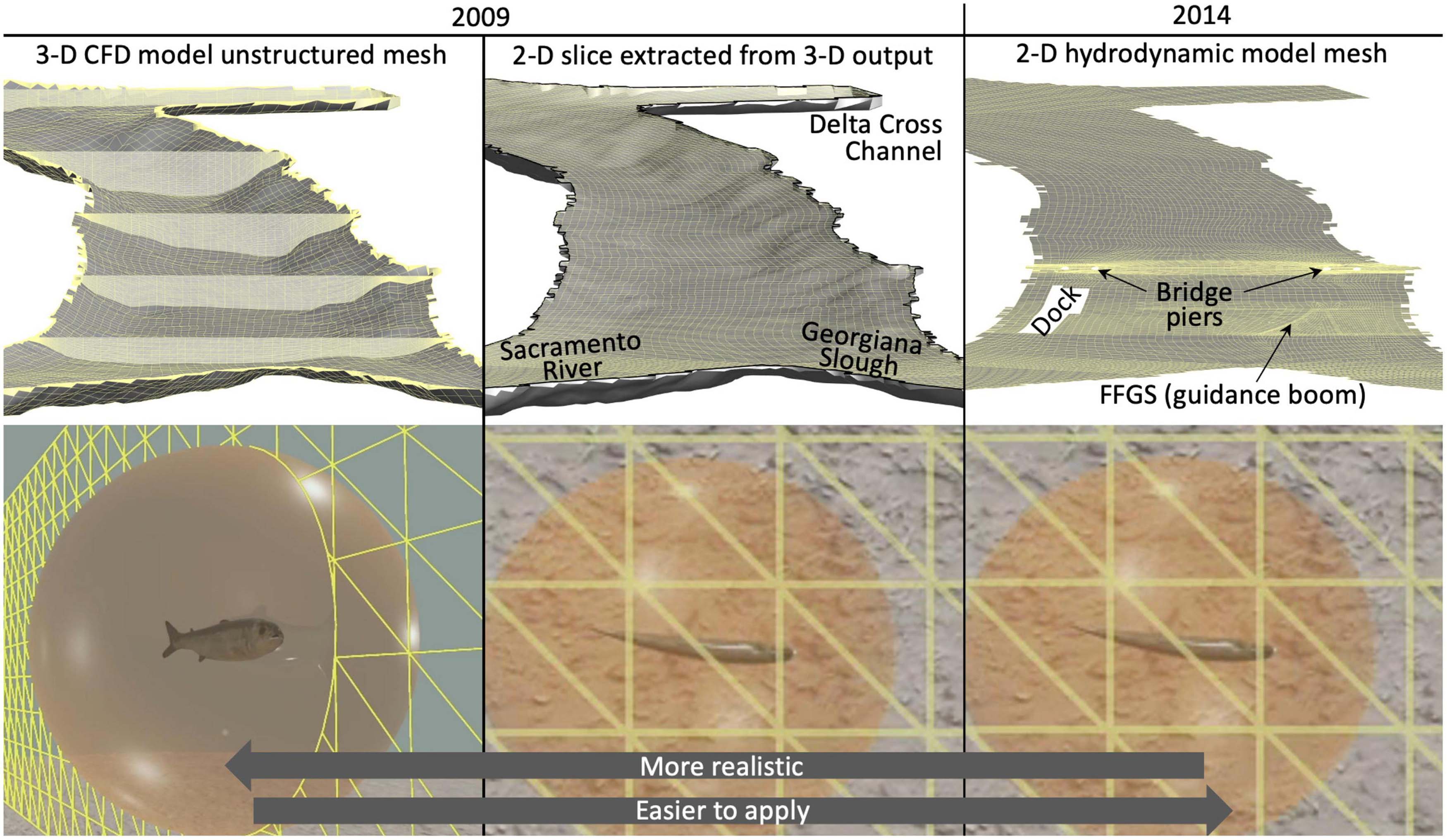
Figure 5. To implement our cognitive approach to mechanistic salmon movement behavior modeling we use a numerical scheme called the Eulerian-Lagrangian-agent method, or ELAM. We use three different forms of river hydrodynamic model mesh output: explicit 3-D hydrodynamics (left panels), 2-D xy-plane horizontal slice extractions from just under the water surface for each output in the original 3-D flow field time series (middle panels), and 2-D depth-averaged water flow fields (right panels). In the 2-D analyses (middle and right panels), both the vertical z-coordinate (depth-oriented) hydrodynamics and fish swim orientation/speed are eliminated. No 3-D model is used for year 2014. Only a 2-D depth-averaged river hydrodynamic model is available for year 2014 ELAM simulations. A sensory ovoid (lower panels) around each simulated salmon limits the spatial extent of stimulus information available for making movement decisions.
• Eulerian — computational mesh (static or time-varying 2-D or 3-D) composed of nodes used to describe the environmental domain;
• Lagrangian — continuous directional trajectory composed of computationally discrete locations used to describe individual movement trajectories and directional sensory perception;
• agent — algorithm ensemble used to describe the behavioral cognitive decision-making of animals.
We simulate each salmon individually in order to gain their Lagrangian perspective. Each individual has agent-based perceptual responses to the Eulerian-meshed river hydrodynamics. A sensory ovoid around each simulated salmon (Figure 5), described in detail later, limits the spatial extent of stimulus information available for making movement decisions. Simulated fish neither have global information nor know downriver from upriver.
In our study, the agent framework encodes our cognitive representation of a salmon’s perceived local hydrodynamic environment and resulting behavioral choices. Fish movement decisions (agent framework) are composed of a swim orientation and speed (Lagrangian framework) implemented in the spatial mesh data output from the hydrodynamic model (Eulerian framework).
3.2.4. ELAM model development and parameterization
To build a hypothesis for the salmon’s behavior repertoire, we identify possible strategic and tactical solutions (Anderson, 2002) that individuals of the population may have evolved over time to confront common and critical challenges in order to survive and persist. Behavioral choice observed in one setting may not be relevant to a repeat encounter. Identifying the motivation of animals is an unavoidably subjective exercise with present technology yet important for understanding which modalities may inform a specific movement decision, how their behavior will vary with context, and for extrapolating existing observations to make predictions in other environmental conditions (Mann, 2018, 2020).
We use a systematic, manual exploratory process to develop and parameterize the behavior repertoire. We start by overlaying the time-dynamic environment with fish movement trajectories. Separate, but related, we also plot each trajectory in its entirety atop the most representative water flow condition. The two overlays are then viewed many times repeatedly, leveraging human visual acuity and intuition. The goal of the initial exploratory process is to find and discern repeated movement patterns — and changes in movement patterns — that cannot be readily explained with how passive particles move. The manual process takes time. Ever-maturing tools are getting better at automating the identification of trajectory patterns and change phenomena (Romine et al., 2014; Gurarie et al., 2017; Vilk et al., 2022). However, we find that to date automated methods cannot yet fully match the performance of human visual acuity and intuition. One reason is that key patterns we find useful for discerning a behavior repertoire are obvious only in the context of — that is, contrasted with — movement dynamics that happen elsewhere either spatially in the domain or in time within the available data.
Unfortunately, we find that key movement patterns and attributes (e.g., changes in swim path orientations) are rarely evident at first and emerge to the human eye/intuition after gaining a gist of the movement patterns and changes. Complicating the process of identifying key patterns and changes is that one must keep in mind the underlying hydrodynamics and what passive particles would do. In rivers, hydrodynamics can vary quickly in both space and time.
An observed real-world fish movement pattern (or change) may have a place in the behavior repertoire if it occurs analogously among multiple individuals. We often observe patterned phenomena of interest to our analysis where hydrodynamic features are more complex. A pattern or change may not have a place in the repertoire if the trajectory could be attributed to inherent animal movement stochasticity, observed in very few individuals, or not coincident with any nearby rendered environmental feature. More complicated is when water flow pattern changes in time, switching from identifiable hydrodynamic features at one moment to perhaps none at all, for instance, during slack tide; in such circumstances, movement pattern changes might be related to the temporal and not spatial domain. Further complicating the process, but where manual acuity and intuition are helpful, is when patterns are obscured by imperfect real-world sampling of the trajectory, common in the aquatic realm. Despite the above challenges, we anticipate that tools in the near-future will automate the present manual process in a way that is more on par with human visual acuity and intuition.
After key distinct patterns are discerned within the trajectory data, typically about a half-dozen, trial-and-error exploration commences whereby one pattern or change is selected and work begins to reproduce that phenomenon using the available environmental data. Once successful, a scaffolding process begins whereby the next distinct pattern or change is reproduced whilst not losing the model’s ability to also reproduce the first behavior phenomenon. Each addition to the model’s behavior repertoire typically involves nuancing the algorithms and parameterization of already-described phenomenon. The exploratory model development process ends with a behavior repertoire, algorithms, and parameterization when all of the identified trajectory pattern and change phenomena can be reproduced with a single structure.
We use prior ELAM model findings as a starting point and guide (Goodwin, 2004; Goodwin et al., 2006, 2014) for how hydrodynamic stimuli might relate to fish movement patterns and changes. We also leverage findings — both old and new — from fish-flow research (Tables 1, 3). In this study, we identify the following four movement patterns and changes in the 2009 data that, once reproduced via simulation, result in the fully developed and parameterized version of the ELAM model described herein:
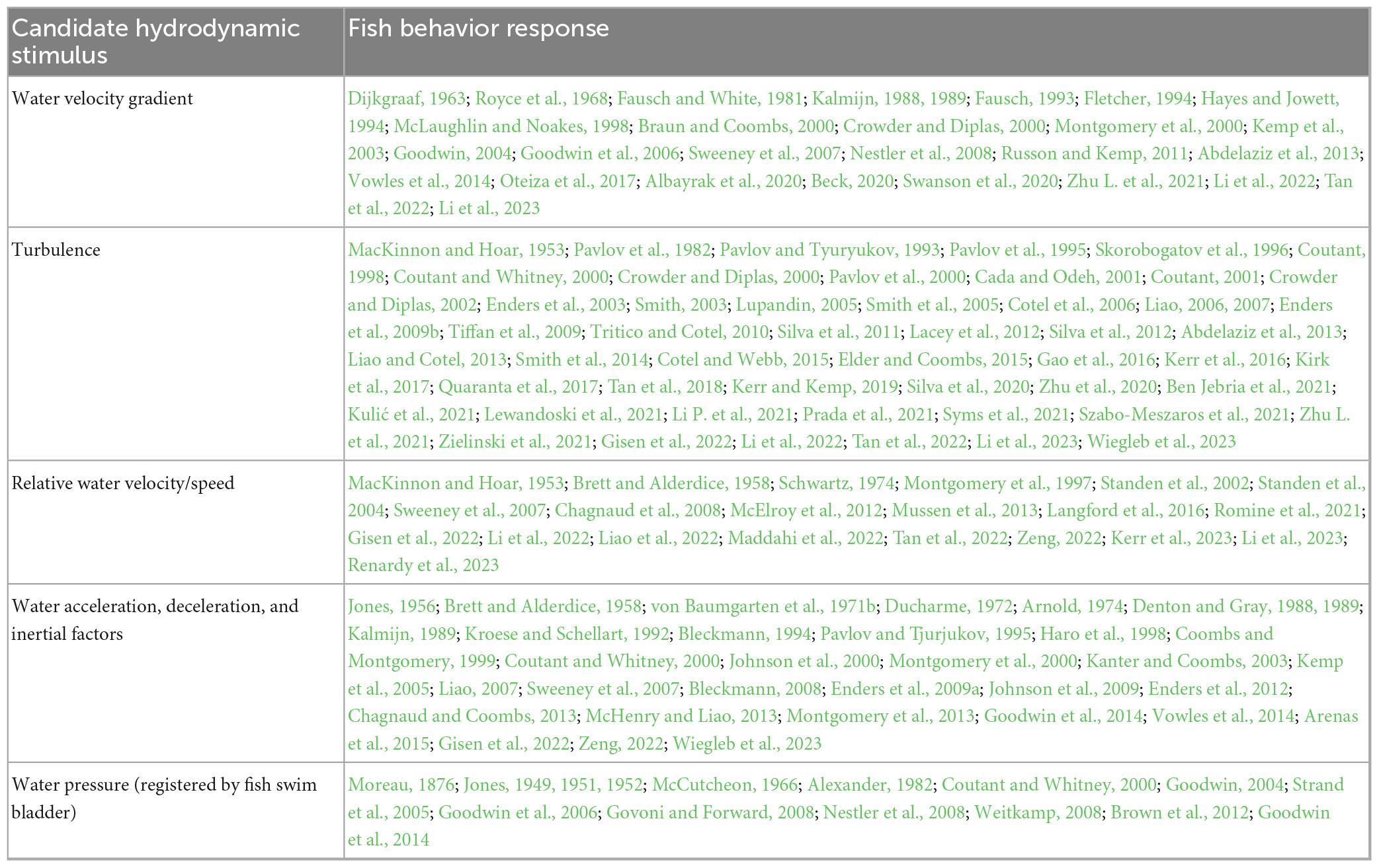
Table 3. Candidate hydrodynamic stimuli: abbreviated synopsis of historical and more recent works.
• a salmon changing its zig-zag within the Sacramento River in front of the Delta Cross Channel junction during relatively steady (unchanging with time) ebb tide flow, suggesting the riverbank per se may not explicitly be solely responsible for the swim path re-orientation pattern;
• nine salmon near-concurrently zig-zagging within the Sacramento River with little-to-no milling in the reach from the Delta Cross Channel to downriver of the Georgiana Slough junction during relatively steady ebb tide flow, in which both flow and fish continue primarily via the Sacramento River;
• two salmon milling, in part, with zig-zag movements during relatively slow flood tide flow, one in the thalweg near the bridge piers and, at the same time, the other along the Sacramento River bank opposite the Delta Cross Channel;
• two salmon milling, in part, with zig-zag movements during relatively slow ebb tide flow into Georgiana Slough, one of the fish in the thalweg just downriver of the Delta Cross Channel junction and the other near the bridge piers that does not enter (e.g., seems to avoid) Georgiana Slough dissimilar from a passive particle. At the same time, two salmon swim upriver in Sacramento River flood flow from downriver of the slough junction and these fish readily enter Georgiana Slough akin to passive particles.
We identify one additional pattern, i.e., two salmon zig-zagging into Georgiana Slough, but are able to reproduce this last example as an emergent outcome of reproducing the previous four examples. The example patterns and changes above are found multiple times in the field telemetry data. Reproducing the above movement patterns via simulation by adding them to the model mix, one by one, is how we develop and parameterize the ELAM in this study.
In due diligence, we rigorously evaluate the model structure and all our parameters that we describe in the coming sections via genetic algorithm and simulated annealing optimization schemes. We evaluate model structure by eliminating (zeroing-out) different components and stochasticity required to initially meet our goal. We also evaluate adding in (activating) stochasticity permissible from the algorithms in our model but not leveraged in the original manual development. Lastly, we explore the model’s parameter space to find optima that may have eluded the manual means of development. Optimization schemes result in no further model or performance improvements but remain an area of study. We anticipate that automated methods will be superior in the future, so the exploratory process leading to the model structure described in the following sections can be accomplished faster and cheaper in later works.
3.3. Hydrodynamic stimuli
Identifying variables of the river flow field relevant to fish movement behavior has been an ongoing process for almost a century (Tables 1, 3). Fish have multiple sensory modalities to inform movement (Liao, 2007), and the context-dependencies in multisensory information are important even for the relatively simple case of rheotaxis (Bak-Coleman et al., 2013; Coombs et al., 2020).
Selecting stimuli for analysis is still unavoidably subjective as the metrics available change with measurement scale. Also, hydrodynamic variables are often correlated. Not surprisingly, different hydrodynamic variables have been attributed to fish movement behavior. We select five candidate hydrodynamic stimuli from the literature for evaluation in our study (Table 3).
3.3.1. Variable physical quantities
A nerve response in fish can be stimulated with relative flow field currents as small as 0.025 mm s−1 (Schwartz, 1974) and water particle movement of less than 0.5 μm (Suckling and Suckling, 1964; Anderson and Enger, 1968; Popper and Carlson, 1998). Fish detect and interact with hydrodynamics at scales far smaller than are rendered in a river reach size RANS model (Borazjani and Sotiropoulos, 2008, 2009, 2010; Windsor et al., 2010a,b; Oteiza et al., 2017; Khan et al., 2022). However, animals also constantly integrate momentary, noisy stimuli sensory evidence over time and space to infer the state of their environment (Bahl and Engert, 2020; Dragomir et al., 2020; DiBenedetto et al., 2022).
We assume fish can generate a hydrodynamic image of its nearby river environment not dissimilar from RANS-level spatiotemporal resolution by integrating sensory experience over time. We do not explicitly account for how a fish upscales minuscule hydrodynamic experiences to form a RANS-level perception of its localized river flow field. However, later, we describe parameterization of Equation 3 that can upscale point measurements of the RANS solution to perceive much larger, bulk flow changes within the river due to the tides. The minuscule-to-RANS and RANS-to-tidal perception upscaling processes could be analogous. Leveraging our assumptions, we formulate candidate stimuli (Table 3) using output from our RANS hydrodynamic model.
The spatial gradient of water speed or velocity (magnitude, GM, s−1) represents the amount of mechanical distortion in the water flow field (Nestler et al., 2008). Mathematically, GM is computed as the Frobenius or Euclidean norm of the pure normal strain (linear deformation), angular velocity (rotation), and shearing strain (angular deformation) tensors. We compute GM on the Eulerian mesh of the hydrodynamic model with u, v, and w representing the mean or average water velocity vectors at time t:
Turbulence is hard to describe mathematically with a single metric (Tennekes and Lumley, 1972; Tritico and Cotel, 2010; Liao and Cotel, 2013; Crowley et al., 2022). For instance, in the x-coordinate direction, turbulent flow can be conceptually viewed as the instantaneous random fluctuation u′ about the mean u where the total water velocity at a moment in time, umomentary, is:
where u′, v′, and w′ represent the instantaneous water velocities relative to the mean velocities. Of the many options for describing turbulence, we select the metric of turbulent kinetic energy (TKE, m2 s−2) to include in our analysis. TKE is computed as follows:
TKE is computed within our 3-D RANS model using the k−ε turbulence closure method (Harlow and Nakayama, 1968; Launder and Spalding, 1974).
Water speed (VM, m s−1) is simply the magnitude of the mean velocities:
Fish are sensitive to gravity and, thus, also to other acceleratory and inertial stimuli (von Baumgarten et al., 1971a), which we define with the spatial, convective acceleration of water (magnitude, AM, m s−2) as:
Lastly, we assume water pressure registered by the salmon’s swim bladder varies proportionally with depth below the surface (D, m).
3.3.2. Spatial velocity gradient (GM) vs. turbulent kinetic energy (TKE)
The magnitude of the spatial velocity gradient tensor, GM, is the sum of linear deformation (pure normal strain rates), rotation (angular velocities), and angular deformation (shearing strain rates) mechanisms. While the mathematics are more involved, in simple conceptual terms, GM can be viewed as a precursor to turbulence. A velocity gradient, GM, may or may not result in turbulence. TKE reflects turbulence that has actually materialized. The velocity gradient may exist in areas with little-to-no TKE but turbulence is less likely without GM. Variables GM and TKE can be highly correlated. Fish may be attuned not only to turbulence but also the distortion that precedes it (Goodwin, 2004; Nestler et al., 2008).
In our hydrodynamic modeling, turbulence represented as TKE exhibits spatial patterns similar to our velocity gradient metric, GM. The spatial pattern similarities between TKE and GM occur throughout our river domain and tidal phases. From a stimulus modeling point-of-view, the similarities suggest only one of the variables is needed. We select the velocity gradient because, in our modeling and post-processing, the spatial GM patterns are more pronounced than TKE across tidal phases. More specifically, the velocity gradient GM illuminates a marked stimulus in areas where tagged salmon re-orient whilst little-to-no TKE signature exists (i.e., down to the lowest practical numerical precision) (Figure 6).
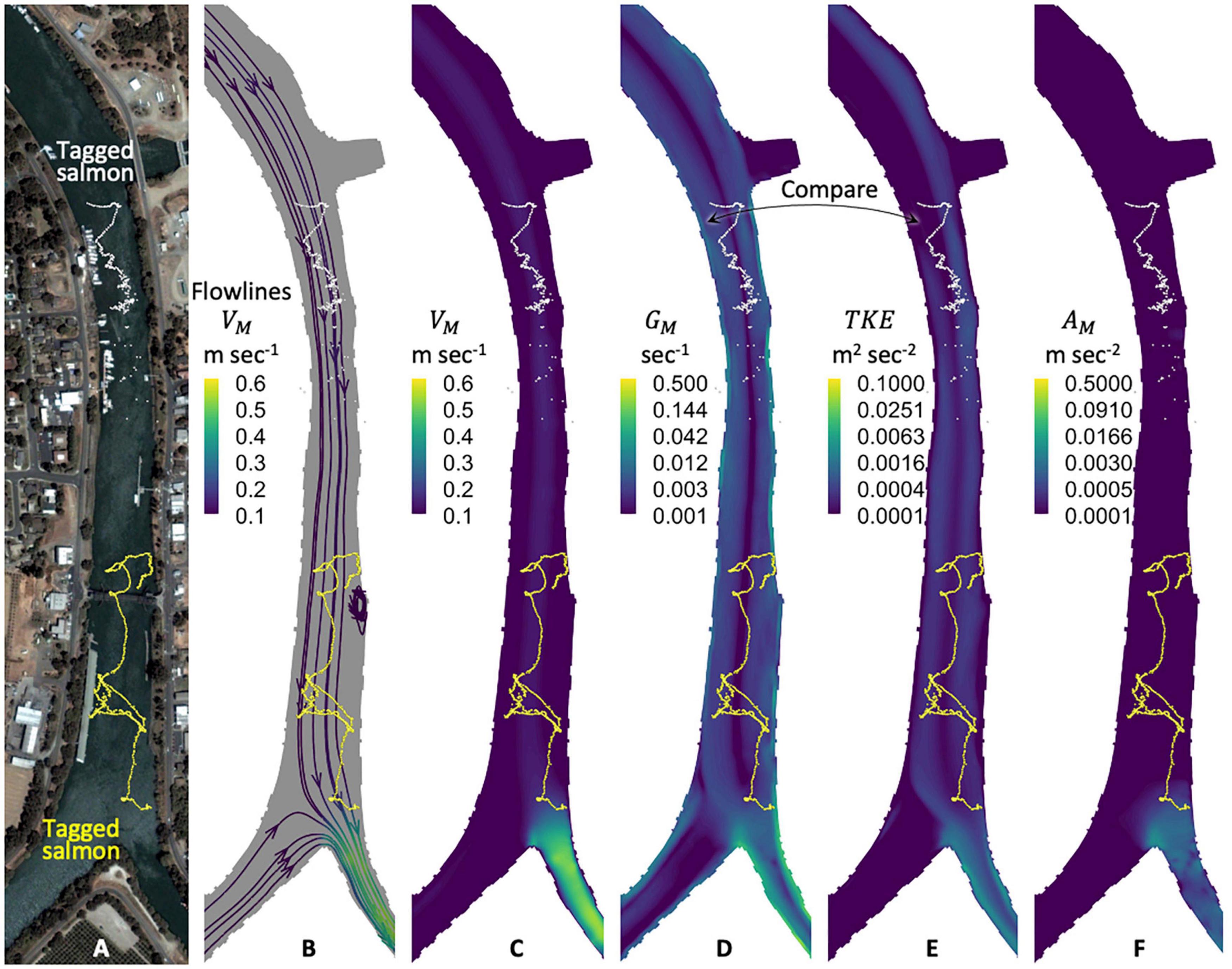
Figure 6. Tagged salmon and candidate hydrodynamic stimuli. Depicted are two tagged salmon (A), water flowlines (B), and the physical quantities of our candidate hydrodynamic stimuli (C–F) in a river scenario with both ebb and flood flows. Spatial patterns in our velocity gradient metric GM are similar yet more pronounced than turbulent kinetic energy, TKE, [compare panels (D) and (E)]. Across tidal phases, GM illuminates a hydrodynamic stimulus in areas where tagged salmon re-orient even where little-to-no TKE signature exists down to the lowest practical numerical model precision available. Map data: Google, Maxar Technologies, U.S. Geological Survey, USDA Farm Service Agency.
Given that fish movement is commonly analyzed in the context of turbulence (Table 3), we illustrate TKE for visual comparative purposes. A full accounting of the tradeoffs between TKE and GM as a behavioral stimulus is beyond the scope of the work herein. We recognize that our TKE finding may be attributable to nuances and idiosyncrasies of our hydrodynamic modeling that, if done differently, might result in a different conclusion regarding the value of turbulent kinetic energy for modeling salmon swimming behavior. The tradeoffs between TKE and GM are worthy of future, more in-depth analysis.
3.3.3. Acute vs. nonacute
We select four hydrodynamic variables to continue our analysis, and introduce the notion of acute and nonacute to conceptually differentiate how the stimuli contribute to and rank in precedence order within a repertoire of multiple competing behaviors:
• spatial gradient of water speed, GM, stimulus i = 1 (nonacute)
• water speed, VM, stimulus i = 2 (nonacute)
• water acceleration, AM, stimulus i = 3 (acute)
• fish swim bladder pressure, D, stimulus i = 4 (acute)
We consider a variable to be acute if the stimulus has a surmised inherent value to the animal across different contexts. Examples include an approaching predator or a physiologically damaging hydraulic condition. In our approach, acute stimuli require a timely response and quickly dominate other, nonacute factors. We consider a stimulus to be nonacute if the behavior’s value to the animal depends mostly on the present context of competing stimuli. The behavior response to an acute stimulus will be more consistent across different environmental contexts as it is less sensitive to competing stimuli. We describe in detail later how competing acute stimulus responses are resolved.
3.4. Stimuli: physical vs. perceived intensity
In rivers, GM and AM quantities span orders of magnitude, so we convert the intensities to log form analogous to the decibel scale using Equation (1):
where Go = 1e−6 and Ao = 1e−6 are arbitrary reference values. Values of VM and D do not span orders of magnitude, so they remain unmodified from their physical quantities:
3.5. Stimuli: perceived change in intensity
We compute the derivative stimulus quantities of GM, VM, and AM on the Eulerian mesh (Equations 11–15), then transform them to perceived intensity Ii (Equations 1, 16–19), and lastly compute the temporal rate of change in Ii at the fish centroid via Equation 2. To be clear, note that we are first computing the derivative quantities of GM, VM, and AM throughout the entire spatial domain as a preprocessing step, in other words, via a global Eulerian perspective. Second, we interpolate each physical derivative quantity from the Eulerian mesh to the precise fish centroid location and transform GM, VM, and AM to their perceived intensity via Equations 16–19. For the last step, we compute one more rate of change (derivative, differential) that is of the temporal domain and conducted only at the fish centroid location. The last derivative uses a local (Lagrangian) perspective in which the individual compares the momentary experience at the fish centroid to a habituated memory integrating all preceding experiences (Equation 2). We describe the last derivative (rate of change, differential) computed at the individual level next, in the following paragraphs.
We find that the perceived change in stimuli i = 1, 2, 3 follow Equation 2 as expected, reinforcing the notion that proportional differencing (signal-to-background ratios) influence behavioral choice. We find again here — as in prior work (Goodwin, 2004; Goodwin et al., 2006, 2014) — that the perceived change in swim bladder pressure (D, m, stimulus i = 4) for eliciting the needed vertical movement dynamics in our approach is best described without the denominator. Specifically, we find that using the denominator results in an asymmetric response to perceived depth changes that biases the modeled fish to move up more than down in the water column. The bias makes it difficult to reproduce observed salmon swim paths. Thus, here as in previous work, we use a simpler formulation that does not bias vertical movement either up or down in the water column:
Alternative methods exist for translating physical (measured/modeled) variables into perceived quantities, Ei, but to date our evaluations have not found better formulations for our stimuli i = 1 − 4 that work across our multiple environmental contexts.
3.6. Multiplex signal disentanglement via multi-timescale perceptions
In our approach, simulated salmon make decisions every 2s even if the choice is no change from the previous time increment. The 2−s time increment is mandated by a goal of keeping individuals responsive to hydrodynamic features that can come-and-go in a matter of a few seconds, e.g., as a fish rapidly transits through infrastructure. Also, we want to limit the number of interactions with the boundary of the hydrodynamic model Eulerian mesh. Regardless of the boundary interaction heuristics employed, e.g., at riverbanks, these features of the model are nonetheless more physical than hydrodynamically-mediated and can, if left unchecked, influence the fate of simulated fish. Our goal is to maintain as much a hydrodynamically-mediated fish swim behavior as possible.
We use memory timescales, mai, to mathematically develop a context for behavioral choice. A timescale is one part of a process that determines the spatiotemporal scales within which a simulated salmon can robustly discern hydrodynamic feature changes. The sequence of perceptual processing (model variables) that results in a behavior decision B is as follows:
In the remaining portion of this section, we describe the first half of the sequence: mai → Iai → Ei. We start with the construct of one timescale for each stimulus i that we refer to arbitrarily as slow. We set (T50 = 3.85 h) where T50 is the half-life of the habituation indicating how long it takes for the level to decline 50% after the last non-zero stimulus acquisition. The memory value is pulled directly from prior work that focused on simplifying the parameter (Goodwin et al., 2014).
We find the single timescale is sufficient for activating a response to our acute stimuli (Table 4) across diverse contexts. We describe the behaviors fully in the next section (Table 5), but for the purposes of illustrating the first part of the perceptual processing sequence we note that one of our behaviors, B{4}, is a response to water acceleration. Most often the behavior B{4} is triggered in the context of simulated salmon avoiding Georgiana Slough, that is, repulsed by the water acceleration enveloping the entrance to the slough. The B{4} response is relatively consistent so long as the water acceleration stimulus, AM, is present at sufficient intensity.
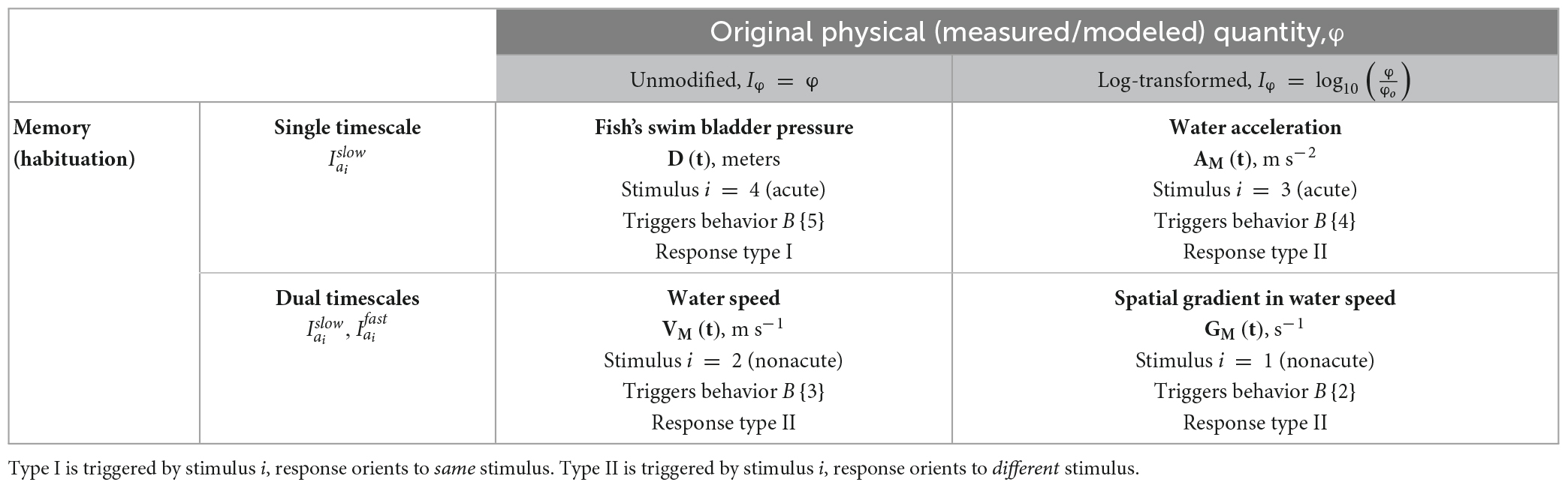
Table 4. Relationship between hydrodynamic stimuli, memory timescales (slow = longer-term; fast = shorter-term), and behavior response.
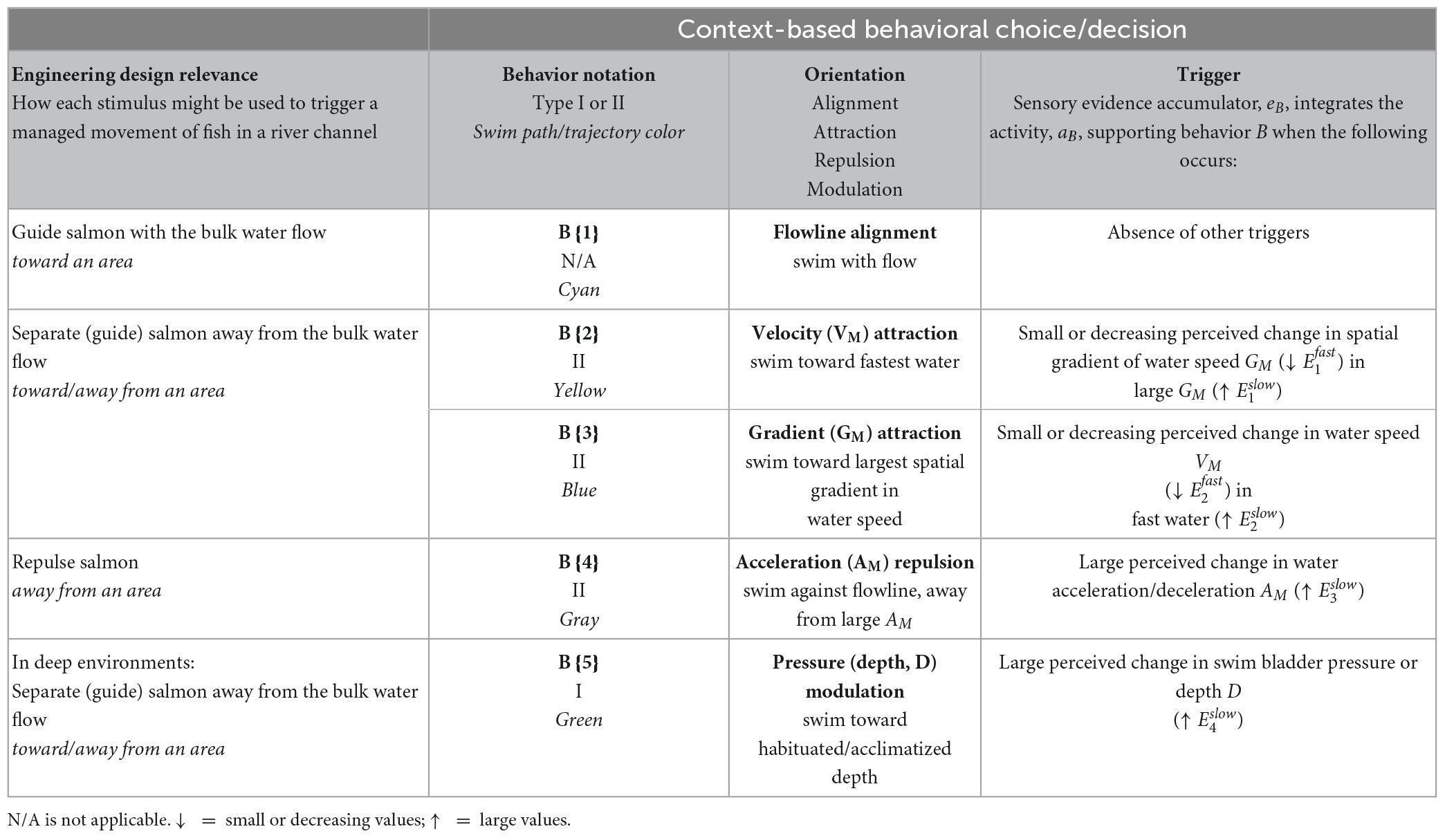
Table 5. Engineering design relevance of each behavior in the repertoire of downstream-migrating salmon responses to river hydrodynamics.
In contrast, we find that responses to our nonacute stimuli — behaviors B{2} and B{3} also referred to with the notation B{2, 3} — require additional context quantification. B{2} is a reaction to GM that results in an orientation toward (attraction to) the fastest nearby water, VM. Behavior B{3} is similar but inverted, in which the response to VM results in an orientation toward the largest nearby spatial gradient in water speed, GM (Table 5). By nearby we mean within the perceptual range of the sensory ovoid (Figure 5) described in detail later. We highlight B{2, 3} here because of their unique dependence on multiple timescales. B{2, 3} must be responsive to both local spatiotemporal features such as riverbank-induced hydrodynamic patterns of elevated GM and low VM as well as to, at the same time, bulk water flow speed changes due to the tides. B{2, 3} take on a very different character — visual trajectory appearance — near the riverbank when bulk river flow changes due to the tides. We find that B{2, 3} cannot be responsive to both localized and tidally-driven bulk flow hydrodynamics at the same time with only a single timescale.
The inadequacy of a single timescale for B{2, 3} precipitates our need for a second that can facilitate perception at a different scale. Equation [3] with timescale (T50 = 3.85 h) forms the basis we need for a simulated fish to perceive bulk flow changes within the river due to the tides; this is the process we alluded to earlier (Section 3.3.1) that may have analogies for how a fish could upscale minuscule hydrodynamic experiences to form a RANS-level perception of its localized river flow field. We pursue a second timescale that can operate at smaller spatiotemporal scales. For simplicity, we start with the length of time between consecutive behavioral choices in our fish model (T50 = 2 s, ) and then evaluate values higher and lower than our initial guess. We find that T50 = 2 s provides the most robust perception of local hydrodynamic features needed to activate B{2, 3}. The superior performance of T50 = 2 s stems, in part, from the intrinsic relationship to our model’s time step that, in turn, is related to the spatial resolution of the Eulerian mesh data. Therefore, T50 = 2 s is not reflective of real fish memory of local hydrodynamic features but, rather, an artifact that is inseparable from our river hydrodynamic description. The dual timescales facilitate perception of hydrodynamic features in our river reach at two different spatiotemporal scales, simultaneously.
Sensory experience for each stimulus i is integrated over time in the form of habituation, and, for B{2, 3}, also . A simulated fish detects perceived changes and by comparing the perceived stimulus intensity at momentary time t to an integrated value over time that corresponds to longer-term (slower, ) and shorter-term (faster, ) habituations, respectively.
A change in water acceleration AM (i = 3) is perceived using the slow timescale (Table 4) via Equation 2:
and swim bladder pressure (i = 4) changes are perceived via Equation 20 using the variation of:
We use two timescales to perceive the velocity gradient GM (i = 1) and water speed VM (i = 2). We expand Equation 2, one for the slow and another for the fast timescale. Perceived changes in GM and VM are perceived in both slow and fast timescales as:
Note the difference between Equations 24 and 2, 21, 23, 25. Equations 2, 21, 23, 25 all follow the same logic structure where the momentary perceived intensity Ii is located in the first position of the numerator. In contrast, Equation 24 places the fast memory (shorter-term) habituation, , in the position. In other words, for VM (Equation 24 only) we modify the slow memory structure of E2 by substituting in lieu of I2 in the numerator. Through trial-and-error, we find that Equation 24 is superior within our modeling approach for an immersed individual to perceive meaningful large spatiotemporal scale changes in river water speed due to the tides.
The floor of habituated intensities for GM and AM are set to 0.001 and 0.0001, respectively. In other words, Iai = 1 ≥ 0.001 and Iai = 3 ≥ 0.0001. Note the numerical floors here are different than the arbitrary reference values of Go = 1e−6 and Ao = 1e−6 used in log-transforming these physical quantities to perceived intensities Ii = 1 and Ii = 3, respectively, in Equations 16,17.
3.7. Repertoire of hydrodynamic response behaviors
In this section, we describe the behaviors so that in the next section we can describe the second half of the perceptual processing (model variables) sequence: Ei,ki → aB → eB → B. We refer to the behaviors B{1}, B{2}, B{3}, B{4}, and B{5} using the notation B{1, 2, 3, 4, 5} and analogously for any subset of responses. Our salmon behaviors B{1,2,3,4,5} are repulsion, alignment, attraction, and modulation responses to the river’s hydrodynamic field (Table 5). The default behavior, B{1}, is swimming oriented aligned with (parallel to) the river flowline facing downstream. B{1} is a negatively rheotactic response that occurs in the absence of stimuli supporting other actions. Behaviors B{2, 3} are both attraction responses, towards faster water and larger spatial gradients in water speed, respectively. Behavior B{4} is also aligned parallel to the river flowline but in the opposite direction facing into, instead of with, the water current where the fish’s head is upstream of the tail. B{4} is a positively rheotactic response to avoid (repulsion from) elevated AM. Behavior B{5} modulates swim depth, D, to mitigate rapid changes in swim bladder pressure.
Only one behavior from the options of B{1,2,3,4} is implemented per time increment △t. The exception is B{5}, which is a vertical-only behavior and always acts in concert simultaneously with one of the behaviors from B{1,2,3,4} that provides the xy-plane orientation. Behavior B{5} is a vertically-oriented response inclined off the horizontal xy-plane. The horizontal xy-plane is perpendicular to the direction of gravity. Since B{5} confers no orientation within the xy-plane — and the fish must always be oriented in some way within the xy-plane — that information is provided by one of the behaviors from B{1,2,3,4}. The orienting process works as follows: first, the simulated fish chooses one of the behaviors from B{1,2,3,4} using the process steps in Table 6 and described in the sections that follow. Second, the simulated fish determines whether a vertically-oriented B{5} inclination is warranted; if so, then B{5} overrides (supersedes) the vertical angle inclination off the xy-plane set by the chosen behavior from B{1,2,3,4}. For example, assume the simulated fish chooses B{4} and this behavior turns (re-orients) their body 5° to the left from the present heading and upward vertically 10° off the xy-plane. Then assume the fish determines B{5} is warranted with a downward angle of 20°. Behavior B{4} and B{5} orientations are integrated as follows: the B{5} downward angle of 20° supersedes the upward 10° inclination of B{4}. Behavior B{5} does not modify the xy-plane 5° left turn (re-orientation) of B{4}. For reference, 0° in the localized xy-plane used in decision-making always points in the direction from the fish’s tail to head.
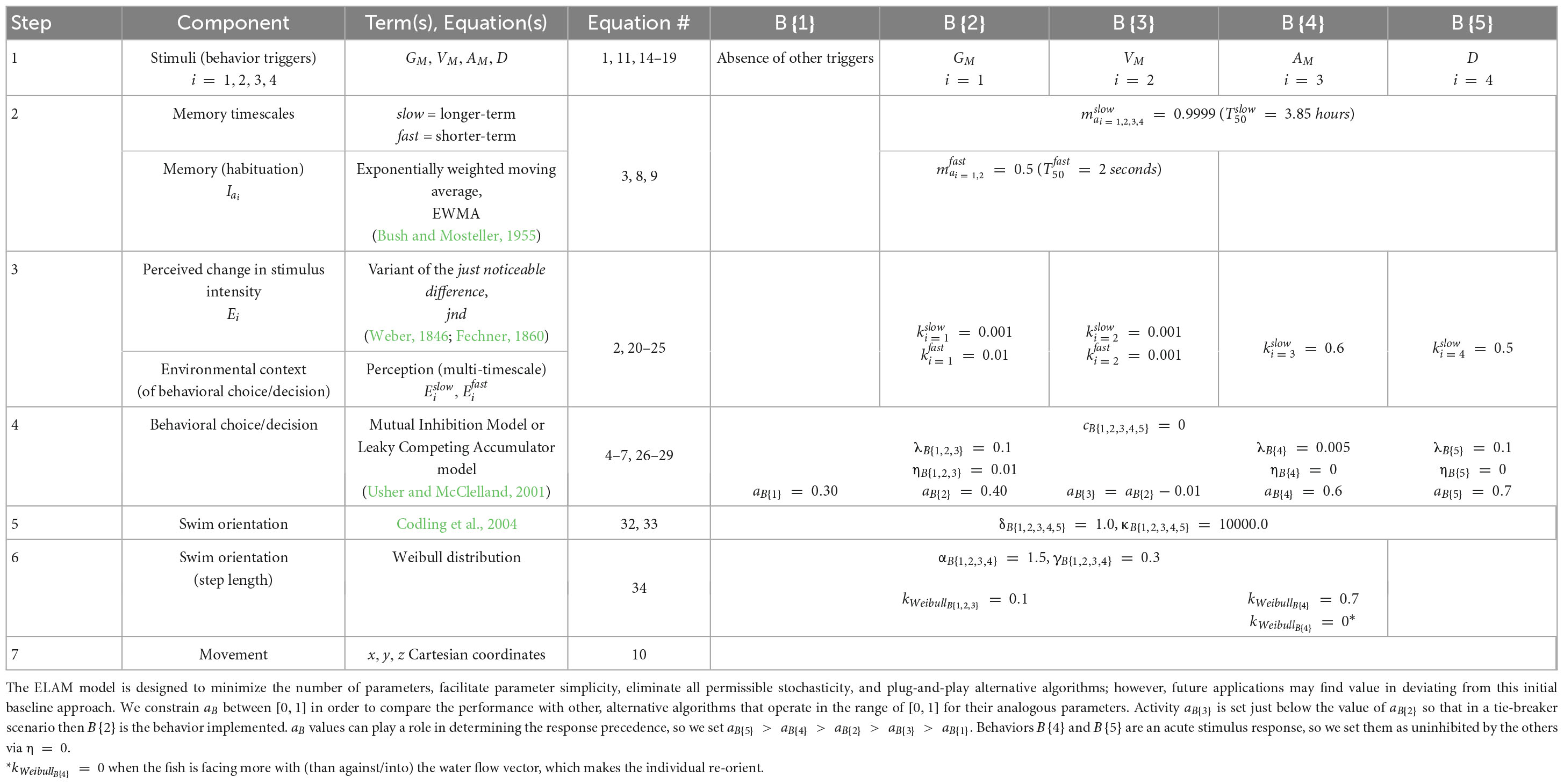
Table 6. Cognitive-based mechanistic fish movement behavior model: algorithm ensemble, steps, equations, and parameters.
Behaviors B{2, 3} often operate in tandem, in opposing fashion, yielding emergent properties that we describe next.
3.7.1. Emergent properties from opposing behaviors
Juvenile Pacific salmon are prey that must reach the ocean in limited time. We propose that a salmon’s downstream migration strategy involves balancing the opposing goals of:
(i) concealing their presence with B{3} by leveraging GM associated with turbulence, acoustic noise, low visibility (elevated turbidity), and physical cover (Anjum and Tanaka, 2020);
(ii) seeking faster water, B{2}, that expedites the salmon’s downriver journey to the ocean.
Behaviors B{2} and B{3} are at odds as B{2} orients the salmon toward the thalweg, e.g., river center, while B{3} leads toward the river’s edge.
Note that from the Lagrangian perspective of an individual fish, the orientation toward faster water does not have to correspond with the water flow direction and often they do not coincide; for example, near the riverbank, water flow may point downriver (parallel to the riverbank) while the direction pointing toward faster water is in line with the shortest path to the thalweg (perpendicular to the riverbank).
Behaviors B{2, 3} work in combination by mutually inhibiting each other, a dynamic that confers the advantageous emergent properties of keeping salmon responsive to rapidly changing conditions, maintaining downstream progress, and a generally unpredictable position within the river. While the fish does not benefit from the optimum river position of fastest water for downriver migration, the salmon increases its survival probability (Sabal et al., 2020). At an evolutionary scale, the B{2, 3} combination increases the probability of salmon life cycle completion and promotion of the species.
The notion of emergent properties arising from opposing and mutually-inhibiting dynamics is not a novel concept. The mutually inhibiting nature of B{2, 3} shares an analogy with the neural inhibitions that operate at much smaller scale within an animal’s brain (Usher and McClelland, 2001; Sukenik et al., 2021). At a very different scale, turbulence both attracts and repulses fish (Smith, 2003; Smith et al., 2005; Liao and Cotel, 2013). In socially-driven animal swarms, attraction and repulsion dynamics are the basis of individual movement (Couzin et al., 2002, 2005; Ballerini et al., 2008; Lemasson et al., 2009, 2013; Katz et al., 2011).
3.8. Context-based behavioral choice
In this section, we describe the second half of the perceptual processing (model variables) sequence: Ei,ki → aB → eB → B. Multiple stimuli compete to influence movement, so we must organize the hierarchical repertoire of stimulus-responses for the changing phases of a behavioral sequence (Sogard and Olla, 1993; New et al., 2001). In our mechanistic approach, using the Mutual Inhibition Model or Leaky Competing Accumulator model (Usher and McClelland, 2001), the perceived changes Ei are translated into a common currency for comparison across all the different sensory modalities, stimuli i. The common currency is activity, aB, from Equation 5. Activities aB are accumulated as sensory evidence eB that support the triggering of its corresponding behavior. Sensory evidence eB is compared across all the behaviors each time step to choose the response. The behavior with the greatest evidence eB is chosen for the next time increment △t = 2 s (Figure 7 and Table 6).
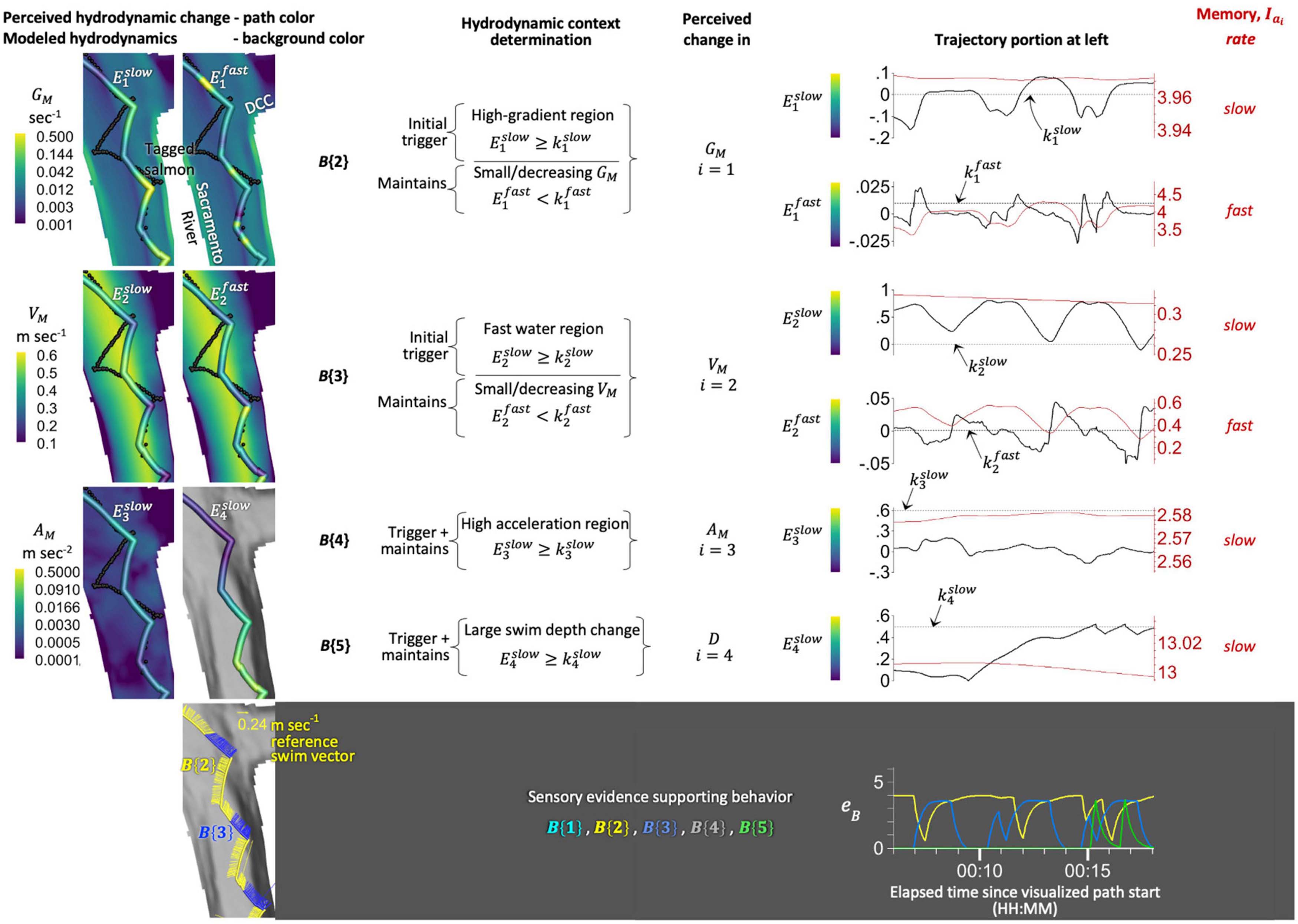
Figure 7. Graphical illustration of a simulated salmon’s perception of river hydrodynamics versus the pattern output by a numerical flow field model, together with the underlying cognitive dynamics of our mechanistic behavior modeling approach. To simplify the illustration, the ELAM salmon is simulated with steady hydrodynamics (unchanging with time) using a snapshot extracted from the flow field time series that is representative of the river flow conditions when the tagged fish was actively swimming. Illustrated are the momentary experiences and behavioral choices of a zig-zagging simulated salmon. The simulated salmon qualitatively resembles the zig-zag movement of a tagged salmon (black path) via behaviors B{2, 3} that arise from perceived changes in VM and GM (Tables 4, 5). Perceived hydrodynamics (Ei, colored path) differ from the river flow field stimulus patterns output from the hydrodynamic model (background color). Additional detail including TKE contours available in Supplementary Figure 1.
In mathematical form, the activity aB − and therefore evidence eB − that supports each behavior B getting triggered increases when the corresponding perceived changes and cross their respective thresholds and . In this way, the fish’s movement decision (swim orientation and speed) is informed by comparing the momentary perceived change to memories of preceding experience. A succinct description of the environmental condition that activates aB and contributes to eB for triggering each behavior B is provided in the right column of Table 5 and illustrated in Figure 7. The process is described in Table 6. We describe the mathematics of how activities aB are computed in the paragraphs that follow.
We constrain the activity constants aB to the range [0.0 < aB ≤ 1.0]. The advantage of constraining activity values is that we can, if ever warranted, compare the cognitive algorithm separate from other parts of our model to other decision methods with parameters also able to operate in the range [0, 1]. We describe the activities aB of the decision-making process starting with behavior B{5}, then B{4}, and lastly the more complicated B{2, 3}.
Activity aB supporting B{5} occurs when the perceived change in depth, D, representing the perceived change in swim bladder pressure exceeds threshold as:
Activity aB supporting behavior B{4} occurs when the perceived change in AM exceeds threshold as:
B{4} and B{5} are acute stimulus responses, and we are able to set these behaviors as uninhibited by the others (η=0 in Equation 5, Table 6). Note that for the acute stimulus responses we are able to simplify the decision process in two ways: first, B{4, 5} require only a single timescale and, second, we are able to eliminate inhibition (η=0).
The activation of the nonacute behaviors B{2} and B{3} is more complex in three ways. First, B{2, 3} require evaluation at two timescales. The slow timescale resolves hydrodynamic features that are generally attributable to the tidal cycle. The fast timescale resolves local features such as riverbank-induced hydrodynamics. Local features can come-and-go with the tides so, for instance, the riverbank-induced hydrodynamic feature of elevated GM and low VM may be negligible or imperceivable during slack tide whereas the pattern is pronounced in ebb tide. Therefore, the pattern of elevated GM and low VM are reliable for indicating a riverbank and/or shallower habitat only under certain environmental conditions (contexts). Second, activating B{2, 3} depends on the existing behavioral state, B, of the salmon. Third, we find the activities aB need to be inhibited by the other behaviors (η=0.01) to operate properly within the overall repertoire.
To switch to B{2} from any other xy-plane response from the options of B{1,3,4}, the salmon must perceive a high-gradient region where the longer-term (slow) perceived increase in GM is while simultaneously perceiving a very small or decreasing short-term (fast) change in GM of , and this latter condition will sustain B{2} once initiated.
Similarly, the initial switch to B{3} from any other xy-plane response, B{1,2,4}, requires the salmon perceive a longer-term (slow) environmental shift to faster water described mathematically as while simultaneously perceiving a very small or decreasing short-term (fast) change in VM of and the latter condition will sustain B{3} once triggered:
We set the value of activity aB{3} just below that of aB{2} so that in a tie-breaker scenario where both B{2, 3} dominate other behaviors, then B{2} is the one implemented.
Activity aB values play a role in determining the response precedence so we set aB{5} > aB{4} > aB{2} > aB{3} > aB{1}. Acute stimulus responses are the highest priority. B{5} is valued higher in the precedence than B{4} but recall that a vertical angle from B{5} does not override a B{4} xy-plane orientation so, in effect, B{4} remains the highest priority in the horizontal plane.
3.8.1. Zig-zag example of context-based behavioral choice with steady river hydrodynamics
We use a single 3-D output, or snapshot in time, extracted from a river flow field time series in order to ignore, for this example, the additional complexity introduced by time-varying hydrodynamics. Simulated salmon swim orientation and speed responses at 2−s intervals (Figure 7 bottom-left) correspond to momentary perceived changes in each stimulus. Habituation to each stimulus updates at multiple timescales described simply as slow and fast. The propensity, or evidence eB, to respond to AM or D increases when the perceived change in stimulus intensity, or , respectively, exceeds their corresponding threshold, kslow.
The activation of B{2, 3}, eliciting the zig-zag swim path (Figure 7), is more complex than either behaviors B{4, 5} that are responses to stimuli i = 3,4, respectively, because perceived changes in the responsible stimuli GM and VM are integrated at both slow and fast timescales and the activities aB supporting B{2, 3} depend on the existing behavioral state B. If a salmon is implementing a non-B{2} behavior, then the simulated fish must experience a high-GM region () to initiate B{2}. Sustaining B{2} requires only a small or decreasing perceived change in GM (). Similarly, triggering B{3} requires the salmon to experience fast water () and maintaining B{3} requires only a small or decreasing perceived change in water speed (). Initial activation, or triggering, of the behavior requires the maintenance criterion also be met at the initiation moment (Table 5 and Figure 7). Whichever behavior B has the maximum accumulated evidence, eB, is implemented for the 2-s time increment (Figure 7 bottom). B{1} is a default behavior that occurs during the absence of evidence supporting other behaviors.
3.9. Sensory ovoid and points
Simulated salmon sense their 3-D environment using a localized sensory ovoid (Figure 5) beyond which the fish has no knowledge of the virtual world. We represent the ovoid using six sensory points located at the cardinal positions (front, back, left, right, above, below) surrounding the fish. The simulated fish is at the center of the ovoid. We refer to the cardinal point distances on the outer edge of the ovoid as the sensory query distance, SQD. Sensory points, or SQDs, are a simple discretized version of the ovoid that simulated fish use to orient in relation to local spatial patterns in stimuli.
Our ovoid is not used to compute any of the trigger stimuli (Table 5). Recall that our hydrodynamic trigger stimuli are local rates of change in time computed at the fish centroid. Our sensory ovoid is used only for orienting the fish toward the fastest nearby water, B{2}, or toward the largest nearby GM, B{3}, in the detectable range sensed by the cardinal points. Since the orienting stimuli VM and GMare scalar quantities, the direction toward higher values cannot be determined with a simple point measurement at the fish centroid. Orientation toward larger values is determined by comparing VM and GM at the available cardinal endpoint locations on the exterior shell of the sensory ovoid to their values at the fish centroid. Note that B{1,4} orientations can be computed using just the water velocity vectors at the fish centroid, so the sensory ovoid is not used for these behaviors. B{5} operates relative to the vertical (gravity) axis and, here too, the sensory ovoid is not needed.
In the real world, the sensory range of a fish depends on the stimulus (Giske et al., 1998) and the SQD would be proportional to fish size. In our model, for simplicity, ovoid size is the same for imaging VM and GM. The size of our simulated sensory ovoid is determined not by fish size but, rather, the spatial resolution of hydrodynamics within the Eulerian mesh. Sizing the sensory ovoid smaller than the spatial resolution of the river hydrodynamics available in the Eulerian mesh results in the situation where VM and GM have the same value at the outer edge (SQD) as at the fish centroid. When the difference in stimulus values between the centroid and outer edge of the sensory ovoid is less than the numerical precision available from the hydrodynamic model — meaning there are no significant digits — then the simulated fish cannot orient to spatial trends in VM and GM.
The limiting factor determining SQD in computer simulations is the numerical precision of hydrodynamic variable values stored in the time-varying Eulerian mesh of the hydrodynamic model. SQDCFD is the distance between a fish and its sensory point location below which orienting stimulus differences have little-to-no significant digits (Goodwin et al., 2006). A spatial trend computed with SQD < SQDCFD is not only unreliable but often misleading. Therefore, simulated fish require SQD ≥ SQDCFD for orientation, and it is preferable that SQD ≫ SQDCFD.
Our sensory ovoid is a construct that lets us leverage the hydrodynamic model information commensurate with the available spatiotemporal resolution. Orienting stimuli VM and GM increase and decrease in intensity at different spatial rates depending on where the fish is in the river. For instance, in the thalweg, VM and GM may not change much across several meters whereas near the riverbank these variables can often change appreciably in less than a meter. Varying the ovoid size each time step provides simulated fish the ability to discern VM and GM trends of different spatial scales. We find that varying the ovoid each time step is a better way to discern VM and GM spatial trends at different scales compared to, for instance, adjusting the size so that it is proportional to the Eulerian mesh element size at a location. Using our approach, we find that even though the SQD may not be optimally sized to detect a particular spatial trend at a given moment in time, the temporal variation in SQD allows a simulated fish to discern the necessary VM and GM spatial trends within a few time steps at most.
Through trial-and-error on our mesh, we set the SQD so that it changes each time step randomly according to a normal distribution with a mean in the xy-plane of 5.0m, a standard deviation of 1.5, and a minimum radius of 0.1 m. The vertical (z-coordinate) radius has a mean of 0.4m and a standard deviation of 0.1. In our approach, a more sophisticated sensory ovoid is not particularly useful unless accompanied with a concomitant improvement in hydrodynamic resolution. Thus, our use of a sensory ovoid is trivial compared to the fundamental concept in Oteiza et al. (2017).
When orienting in relation to VM and GM spatial trends, one or more of the four xy-plane sensory points must have a |jnd|≥1% in that variable’s value relative to the fish (centroid), otherwise orientation remains unchanged from the previous time increment. A jnd is used here, as opposed to the nsd, because this is a discrete comparison. The 1% rule is constant even as the ovoid size changes each time step. If all cardinal point |jnd| < 1%, then we assume there is no relevant perceived difference or spatial trend in VM or GM around the fish at the scale of time t′s sensory ovoid and hence no orientation change. Vertical sensory points and orientation are handled analogously to the xy-plane.
3.10. Swim orientation
Behavior B determines the preferred orientation, θo. Before we describe the swim orientation algorithm that we use in this study, it is worth noting the Ornstein-Uhlenbeck (O-U) model (Uhlenbeck and Ornstein, 1930) for several reasons. The O-U model is a powerful, longstanding approach to orientation that is used frequently (Gurarie et al., 2017), and remains a constant source of evaluation in our own work. The O-U model has attributes similar to Equations 4 and 5 used in other parts of our algorithm ensemble for cognitively deciding individual behavior transitions. The O-U model describes and produces a stochastic movement orientation that is implemented in the model, θ, based on the idealized preferred direction θo from behavior B as follows:
or as a complete, first-order approximation of the stochastic differential equation in discrete form (Gillespie, 1996; Natvig and Subbey, 2011):
where ζ is a sample value from a standard normal distribution N(μ=0,σ2 = 1) with mean μ and σ standard deviation, ψ is the drift term describing the strength of attraction to the preferred orientation θo, θ′(t) is the orientation at time t, c is a noise-scaling factor analogous to its use in Equations 4 and 5 or it can be thought of as a diffusion term where is the white noise, Brownian motion, or a Wiener process describing randomness. When ψ=0, then there is no attraction to the preferred orientation θo, only diffusion.
We find the mechanics of the Codling et al. (2004) algorithm integrate better with our overall methodology. We use the Codling et al. (2004) algorithm to compute the movement orientation that is actually implemented in the model for a given time step, θ, based on the idealized preferred direction θo from behavior B. In our approach, we use the Codling et al. (2004) algorithm to set the initial movement orientation θ whenever there is an updated preferred direction θo due to a change in behavior B. Since one of our goals is to eliminate all permissible stochasticity, we do not use the algorithm during consecutive orientations when the behavior B is not changing. Should stochasticity during consecutive orientations be required in future work, we find the Codling et al. (2004) and O-U algorithms both suffice.
In the Codling et al. (2004) algorithm, the swim orientation is randomly drawn from a von Mises distribution T(θ,θ′) that is dependent on a concentration parameter, κ, and mean turning angle, μθ−θ′, as follows:
where Jo(κ) is the modified Bessel function of order zero, and the mean turning angle is:
where θ is the movement orientation at time t + △t, θ′ is the movement orientation at time t, and 0 < δ△t is the amplitude of the mean turning angle. δ△t controls how quickly the swimming orientation returns to the preferred direction θo during the re-orientation process, which is a proxy for the sensing ability of the animal (Codling et al., 2004). κ controls the amount of randomness in the choice of each new orientation and is a proxy for the orienting ability of the animal. A low value of κ corresponds to a poor orientating ability, for instance, in a highly turbulent environment. Setting κ=0 collapses the von Mises distribution to a wrapped uniform distribution. μθ−θ′ > 0 biases the random walk in the preferred direction θo (Codling et al., 2004).
3.10.1. Swim orientation (step length)
Swim orientation in our model is further influenced by step length, or re-orientation probability (Okubo, 1980). We use the Weibull distribution to determine the fish’s propensity to maintain the same orientation (step length). The Weibull distribution is often used in fatigue (time-to-failure) analysis as well as in ecology for the analyses of step length in animal movement and correlated random walk models (Morales et al., 2004; McClintock et al., 2012, 2014). We describe the Weibull probability density function (random number) as:
where α is the shape and γ is the scale parameter, respectively, and ζ is a sample value from a standard normal distribution N (μ = 0, σ2 = 1) with mean μ and σ standard deviation (Table 6).
Our use of the Weibull distribution is simple. In our approach, the fish’s orientation is allowed to change based on the preferred direction θo of behavior B if the Weibull random number is greater than or equal to a threshold value, kWeibull, that does not change with time. If Weibull < kWeibull, then the simulated fish’s orientation is not changed (i.e., continues straight-ahead) although the movement trajectory may not be straight because of the contribution from advection due to river hydrodynamics.
We do not apply the step length treatment to the vertical-only behavior, B{5}, but it is applied to the vertical orientation component of all other behaviors that act in 3-D whenever the Eulerian mesh is three-dimensional. Shape and scale parameters of the Weibull distribution as well as the threshold values are set as part of model development and parameterization.
3.11. Swim speed
Simulated fish swimming speed is modulated by both behavior and the environmental condition. The swimming speed for each behavior B is based on a surmised interpretation of the stimulus-response’s value to the animal. For instance, swim speed may be slow, or otherwise bioenergetically efficient, for a default behavior that is executed merely because there is a lack of important stimuli. In contrast, the swim speed may approach the species’ burst propulsion limit for an avoidance response in fast water.
We set swim speed as bodylengths (BL) persecond, or BLs−1, according to drift, cruise, and burst swimming modes (Beamish, 1978) with an assumed juvenile salmon size of 0.12m (120mm). The swim speed of each behavior is set initially as:
• B{1} is a drift swim mode (0.25BL s−1, 0.03 m s−1);
• B{2, 3, 4} are cruise modes (2.0BL s−1, 0.24 m s−1).
If water flow is faster than cruise swimming during an AM avoidance response, B{4}, then swim speed instantly increases to 1.9VM up to the burst maximum of 10.0BL s−1, 1.2 m s−1. The burst speed is near the maximum BL s−1 measured in Bay-Delta juvenile salmon (Lehman et al., 2017).
Vertical swimming, B{5}, depends on the xy-plane behavior where speed is initially set from one of the following B{1,2,3,4} but is increased up to 1.9VM, but no more than the burst maximum, whenever the fish is failing to alleviate recent perceived change in swim bladder pressure. Vertical overrides of the xy-plane behavior speed typically occur when the simulated fish must counteract strong vertical water currents, most common in deep environments near infrastructure.
We simulate all fish identically as 120mm in length even though the mean fork length of tagged fish is slightly higher than 150mm. Our reason is that salmon management is concerned with fish as small as 60mm (California Department of Water Resources, 2016). We arbitrarily select a single fish size between 60 and 150mm, slightly closer to 150mm. We do not use a distribution of fish sizes in order to reduce heterogeneity and stochasticity in the model wherever permissible. The assumed salmon size by itself is not a critical assumption in the model. The same swim speed (m s−1) can be obtained for a different sized fish with simple counterbalanced shifts in the assumed drift, cruise, and burst swimming bodylengthspersecond (BL s−1) values.
3.12. Swim orientation and speed integration
We find one last nuance required of B{2, 3} using the aid of steady ebb tide flow hydrodynamics and the transit times of tagged and modeled salmon within our river reach (Figure 8 upper-right dyad). During ebb tide flow, tagged salmon zig-zag at a travel rate that can only be qualitatively reproduced in simulation if the ELAM fish is partially positive rheotactic, that is, the modeled individual orients their swimming facing slightly into (against) the oncoming water current (see the orientation of the swim vectors in Figure 7 lower-left). Whenever water speed exceeds the fish’s cruise swim speed of 2bodylengthspersecond (Beamish, 1978) we prescribe that the rheotactic orientation of B{2} and B{3} increases positively by 10%. The 10% is only a rheotactic increase in the preferred orientation θo and not an absolute angle relative to the water flow vectors.
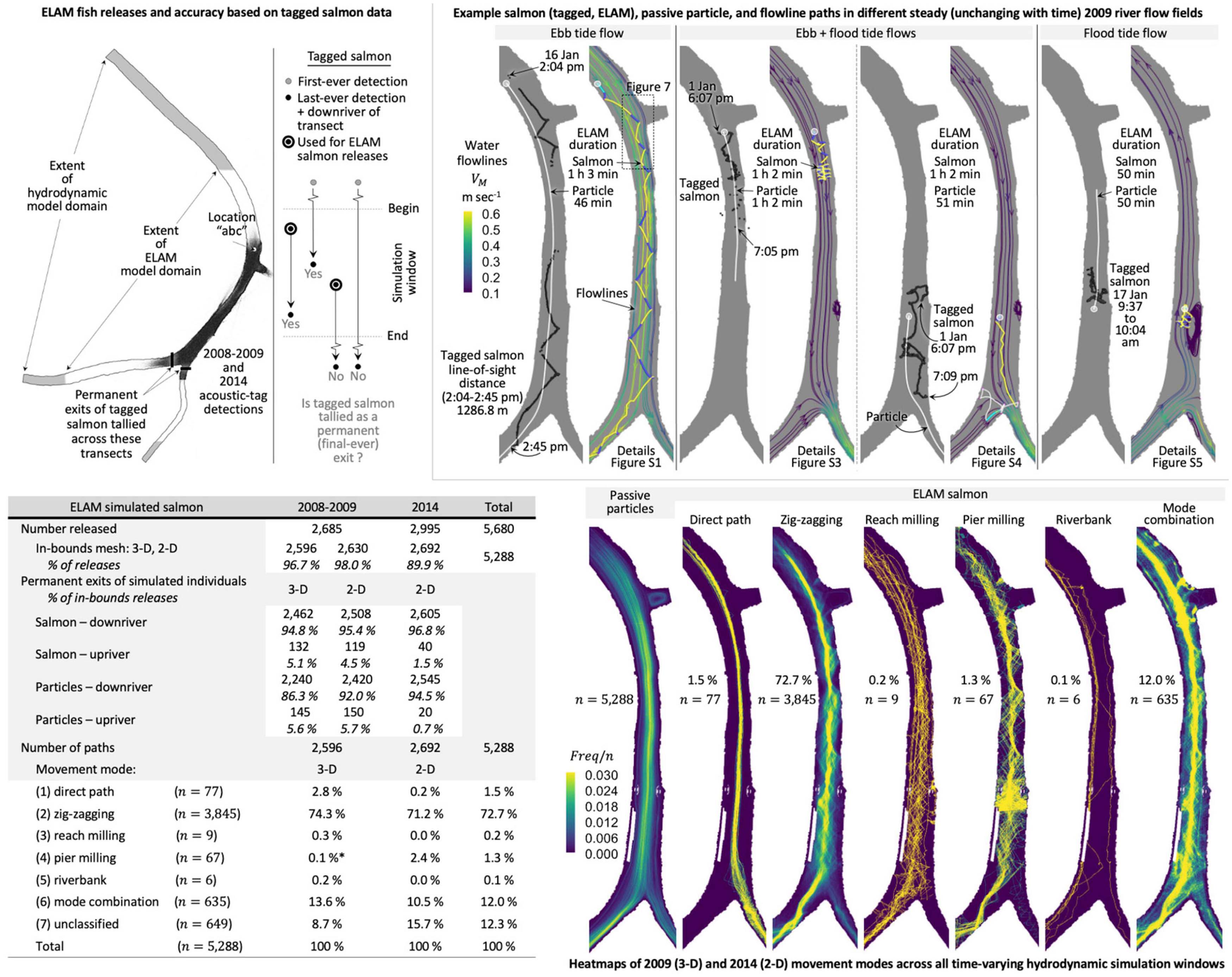
Figure 8. Setup of the ELAM analysis (upper-left), example tagged and simulated salmon paths with a passive particle (upper-right), movement mode heatmaps (lower-right), and tabulated downriver entrainment and movement mode proportions (lower-left). Spatial extent of the hydrodynamic model is based on available river gage (Figure 1) and bathymetric data. ELAM model spatial domain is based on the extent of salmon acoustic-tag telemetry data from 2008 to 2009 (Romine et al., 2013) and 2014 (California Department of Water Resources, 2016; Romine et al., 2017). Tagged salmon exits are used to assess the accuracy of simulated individual (particle, salmon) entrainment. Example swim paths of tagged salmon (black path) and ELAM fish (path colored by behavior B, Tables 4, 5) are provided in dyads for different tidal environments (ebb, flood, ebb+flood tide flows), which can be compared to the passive particle (white path). The example simulated particle and salmon paths within each dyad are released from the same location (white circle) near where the tagged fish is first detected. The ELAM salmon and particle are simulated with steady hydrodynamics (unchanging with time) using a snapshot extracted from the flow field time series that is representative of the river flow conditions when the tagged fish was actively swimming. The underlying cognitive dynamics of each example ELAM salmon are illustrated in greater detail in Supplementary Figures 1, 3–5 along with candidate stimulus TKE. Heatmaps are generated from the simulated individuals (particles, salmon) responding to time-varying hydrodynamics changing every 3min across all simulation windows. Heatmap values are computed the same as in Figure 3 and, just as in Figure 3, only modeled fish detections are heatmapped, that is, the paths are not implied from the position sequence. Note that modeled individuals are detected perfectly at 2-s increments throughout the domain, unlike tagged salmon. One reason why simulated salmon exhibit less milling near the piers (movement mode #4) in year 2009 (*) compared to year 2014 may be that the bridge is not rendered in the 2009 mesh (Figure 5) and, thus, its hydrodynamic impact on the river is not perceivable to ELAM salmon.
In behavior rule computations thus far, the simulated fish’s 3-D orientation is based on a local coordinate system tied to the direction in which the salmon is pointing its head, which can change every time increment. In the xy-plane of the local (fish heading) coordinate system, 0° is straight-ahead, 180° is behind the individual, 90° is to the left, and 90° (or 270°) is to the right of the individual. Water pressure (depth) varies parallel with gravity, so we maintain the local and global vertical coordinate systems as the same. When the local 3-D orientation and swim speed is computed, we can then use how the salmon is oriented in the global Cartesian mesh of the Eulerian-based hydrodynamic model to compute the component swim vectors uvolitional, vvolitional, and wvolitional, which completes the spatial displacement Equation 10.
3.13. Model time step
We find that simulated salmon need to make movement decisions at 2−s increments in order to react quickly in fast water. Longer time steps increase the number of mesh boundary encounters as well as scenarios where simulated salmon are hydrodynamically captured (entrained) that, by contrast, tagged fish successfully avoid. Depending on the scenario, our cognitive algorithm ensemble generally requires several discrete time steps for an acute stimulus response to rise within the hierarchy of competing behaviors and enable the simulated fish to successfully realize an aversive maneuver before capture. We find that 2s is the longest increment permissible for the requisite number of time steps to occur that allow acute stimulus responses such as B{4} to achieve the avoidance observed in tagged salmon in rapidly-changing hydrodynamics near infrastructure. Thus, the 2−s time step is an upper-bound on the increment length for our river analysis. We forgo smaller time increments because it increases model runtime without a needed benefit for our study setting.
All hydrodynamic values are linearly interpolated spatially from their nearby mesh storage locations (e.g., cell vertex/node, cell center, or cell face center) to the precise fish centroid location and seven surrounding sensory points every 2s. First, all stimulus values are interpolated spatially in linear fashion to the precise fish position and seven sensory points for each of the adjacent 3−min intervals on either side in time from the available hydrodynamic model output. Then, second, stimulus values are linearly interpolated to the 2−s increment of the fish’s decision moment from the adjacent 3−min interval values.
Most parameters of the fish cognition algorithm ensemble (Table 6) are intrinsically linked to the time step increment in their present form. Changes to increment length require counterbalancing other parameter values in order to compensate and retain the same cognitive dynamics achieved with another step length. Parameter re-balancing, however, occurs in a nonlinear, multidimensional space that can be challenging to negotiate. Practically, changing the time increment length usually involves recalibrating the model. Insulating model performance from increment length may be possible as a future improvement and, presently, may be found in limited form in components such as swim orientation step length.
3.14. Lagrangian encounters with the Eulerian mesh boundary
A key but often overlooked issue that can arise and have large, unintended effects on the destination of simulated volitional individuals in bounded 2-D or 3-D environmental domains is their interaction with the boundary of the computational Eulerian mesh. River hydrodynamic modeling generates the mesh as part of the development process. We simulate fish within the original mesh of the hydrodynamic model in all of our work regardless of element type and geometric mesh tessellation. The hydrodynamic domain has boundaries at the water surface, riverbank, and river bottom. The domain tessellation can change each 3−min timestep, and this is relatively common in modern hydrodynamic models that use adaptive meshing methods.
The behavior repertoire is built and parameterized to make every attempt within reason so that simulated salmon respond only to hydrodynamic stimuli including near boundaries such as the riverbank and bottom bathymetry. Limiting interaction with physical boundaries is a key reason why our timestep is 2s. As a backup for when our simulated fish do physically interact with a boundary, every practical attempt is made to recover hydrodynamically-mediated decisions within a single timestep of the behavior model.
When a fish’s sensory ovoid runs up against a physical boundary in the Eulerian mesh, compressing one of the cardinal point distances toward the fish, the individual is re-oriented away from the feature for that timestep alone. Our model works in double precision, yet even still the numerical processes within a computer are neither infinite nor perfect. Situations arise where double precision calculations store a fish adjacent to a boundary by an infinitesimal distance on the other (dry, non-water) side. Then, at the next timestep, the model interprets the same position as outside the meshed domain. We employ heuristics in an attempt to recover fish violating the boundary by repositioning the individual to the nearest mesh cell center, typically, a very short distance from the point of violation. Hydrodynamic models typically use tessellation methods in which there is a graded approach to cell sizes where they are small near physical boundaries and larger nearer the thalweg or wide unobstructed water flow regions. Therefore, our heuristics generally result in very small location displacements while recovering hydrodynamically-mediated behavior within a single timestep. As a third backup, when the boundary interaction heuristics are insufficient, then the modeled fish is removed from simulation. Removals are seldom. Next, we provide examples of boundary interaction scenarios that do not always have obvious conceptual or computational heuristic solutions.
Mesh boundary encounters in the following scenarios can result in the loss of simulated individuals, at times, depending on the exact circumstances. First, the scenario of a simulated individual in 3-D located near the water surface and riverbank. At the next time step, the water surface drops but simulated movement behavior (an imperfect abstraction of the real world) keeps the individual near the previous xy-position where there is no longer water, or even a mesh if the grid is adaptive. Second, the scenario of two individuals at the same xy-position but at different depths, one at the water surface and one at the river bottom. At the next time step, the water surface drops. If we lower the individual at the water surface to maintain its depth, the one at the bottom cannot be handled similarly because it would then be placed under the river. If we chose to do nothing for the one at the bottom yet lower the individual at the water surface, then the ELAM model now treats simulated individuals differently according to depth — a model complexity that can have unintended consequences. Third, and similar but not exactly the same example as described earlier, the scenario of an individual at the riverbank an n-th decimal place (spatially) inside the river domain. At the next time step, computer precision/truncation results in the individual now an n-th decimal place outside the meshed domain. If the mesh has adapted during the timestep change, then sometimes there is no clear solution heuristic for identifying the most appropriate interior cell in which to place the fish. Fourth, the scenario of an individual in a wetting-and-drying scenario (Lai, 2010) where the Eulerian mesh changes with river inundation and water may not be spatially contiguous at all times near a riverbank or in the floodplain. A simulated individual near the riverbank or in the floodplain can be cut off from the river during drying cycles and find itself trapped with no way out when its refuge dries entirely.
Some of the above issues have robust solutions for passive particles and/or certain types of mesh geometries (tessellations). We want the same boundary encounter heuristics applied across all simulated fish, particles, and 2-D/3-D mesh element shapes to prevent such attributes from contributing to differences between applications. To date, we have found neither an optimum nor computationally-efficient solution heuristic for all combinations of possible mesh tessellation, element shapes, boundary topologies, and time-varying mesh/element/boundary changes that can arise in 2-D and 3-D.
3.15. Synchronizing observed and modeled passage/entrainment
Passage (entrainment) is often a critical biological criterion determining the engineering success of water operations management or the design of an in-river structure. To assess the performance of our approach, we want to quantitatively reproduce the passage/entrainment proportions of tagged salmon using the ELAM model. Synchronizing real and simulated worlds for comparative analysis, however, is not straightforward. Tagged salmon in 2008–2009 (Romine et al., 2013) and 2014 (Romine et al., 2017) may occupy our spatial domain prior to the simulation window and/or remain in the area afterward (Figure 8).
Transects immediately downriver of the junction (Figures 3, 8) are used in our analysis to determine the final passage/entrainment (permanent exits) of tagged salmon (Table 2). The available telemetry data does not afford us the ability to move the transects further downriver. Tagged fish that occupy our domain before the simulation window and remain in the area afterward are not part of our analysis as these individuals represent a movement mode that our model does not attempt to reproduce. Non-downriver movement may be rooted in the tag being eaten by a predator not perfectly filtered previously (Romine et al., 2014), in a dead salmon on the riverbed, or long-duration milling/riverbank movement modes. We only use tagged fish with a predator probability less than 0.85 in the range [0, 1] (Romine et al., 2014) at the time of their final, permanent exit for comparison with modeled entrainment (Figure 3e and Table 2). We do not count tagged fish that linger beyond our simulation window as part of the real-world entrainment proportion regardless of when they enter the domain (Figure 8). However, we do count tagged salmon that permanently exit during our simulation window even if they occupy the area beforehand.
Year 2009 predator probabilities from Romine et al. (2014) are formatted such that we can identify and remove suspected predators at a tag’s first-ever detection (Figures 3d, 8 and Table 2). Year 2014 probabilities are formatted differently, so we assume all initial tag detections are salmon. Tagged salmon detected for the first time in our domain during the simulation windows, but that are not part of the passed/entrained tally are often fish released into Georgiana Slough that remain downriver of the transect; that is, these tagged fish reveal themselves in our domain only within the small spatial region downriver of the transect in Georgiana Slough. Our conceptual tradeoffs result in tagged salmon passage/entrainment into Georgiana Slough and downriver into the Sacramento River that total 100%.
Simulated salmon are tallied as they exit the ELAM model domain downriver of the junction (Figure 8) instead of the transect to allow individuals the opportunity to move upriver back into the junction area and select a different route from their first choice. In this way, the modeled and empirical passage proportions are comparable as it is the final passage decision of the observed (telemetry) fish that are factored. The spatial extent of the ELAM model domain is shortened from the river flow field mesh to more closely align with available telemetry field data (Figure 8). Simulated individuals, salmon or particles, that do not exit downriver (Figure 8) result from one of the following reasons:
• out-of-bounds release;
• mesh boundary interaction requiring removal;
• exits upriver;
• freely remains in the domain.
Simulated salmon exiting the domain at the upstream boundary are not factored into modeled passage/entrainment, which considers only downriver entrainment. Simulated salmon released on a particular day are allowed up through the end of the following day to exit after which they are removed from simulation and labeled as remaining in the domain. We do not attempt to capture the dynamics of salmon that linger in the domain longer than 24−48h. Simulated individuals that remain in the domain are often releases near the end of the simulation window. However, some non-exiting particles are caught in an eddy and swirl in the cul-de-sac of the Delta Cross Channel inlet region, and some salmon exhibiting a riverbank movement mode are removed downriver of the junction due to drying mesh elements.
Simulated individual exits are equivalent to measuring their passage/entrainment at the transects so long as they do not incur a mesh boundary interaction between the transect and domain extent necessitating its removal from simulation. Fish removed due to boundary interaction issues are not considered in passage/entrainment proportions. Our conceptual tradeoffs result in simulated entrainment into Georgiana Slough and downriver into the Sacramento River totaling 100%.
3.16. Release of simulated individuals
Five simulated individuals are released at the location (xy-position) and time of each initial tag detection within our simulation window (Figure 8). We avoid releases associated with tagged fish that have been in the area for days or weeks. Releasing five simulated individuals per tagged salmon is an arbitrary judgment based on balancing model runtime and the replicates needed to average out the required/unavoidable stochasticity in our cognitive algorithm ensemble (Table 6). Replicates also serve as a contingency against losing individuals during simulation from mesh boundary interactions. We believe the above approach makes the best use of our limited field data (Figure 3).
Vertical positions from the underwater acoustic-tag telemetry (z-coordinate values) are not accurate enough to determine water column locations, so we have to artificially generate the release depths at each xy-position. We assume the Sacramento River’s depth is too shallow for salmon to exhibit a lognormal depth profile (Smith et al., 2010; Goodwin et al., 2014). Instead, here, we use a simple normal, or Gaussian, distribution N (μ,σ2) with a mean depth μ = −2.5m and a standard deviation σ=0.75 as follows:
where ζ is a value drawn from the standard normal distribution N(μ=0,σ2 = 1). In some cases, a release is out-of-bounds due to a depth (z-coordinate) generation that is under the river or imprecision in the field telemetry xy-position placing the fish outside the river channel in the xy-plane (Figures 3, 8). In 3-D simulations for year 2009, a release is out-of-bounds if not within the river domain in the horizontal plane at the fish’s depth. In 2-D modeling for year 2009 and 2014, a release is out-of-bounds if not located within the horizontal plane of the river channel as depth does not factor into the simulations. We do not manually modify out-of-bounds release locations to convert them into in-bounds positions. Simulated individuals (salmon or particles) released out-of-bounds are immediately removed from simulation and play no further role in our results.
A minimum proportion of simulated individuals (salmon or particles) must exit the domain downriver within the simulation window for modeled entrainment to be valid in our analysis, either in comparison with real-world patterns or, later, as part of a prediction about the future. We arbitrarily require that the proportion of simulated individuals exiting the domain downriver be greater than the proportion of total tagged salmon exits (Table 2), less ∼10%. In other words, since 86.6% and 85.1% of tagged salmon permanently exit during each seven-day simulation window for year 2009 we require that ≥ 75% of simulated individuals must exit the domain downriver. We require ≥ 35% of simulated fish must exit within each 2014 three- or four-day window (Figure 8) since only 43.0% of tagged salmon permanently exit during the timeframe of 22–24 March. The criteria we use is arbitrary but a useful way to flag and eliminate the use of outcomes where, for example but not encountered in this work, too many modeled fish are removed from simulation due to boundary violations described earlier. If the proportion of downriver domain exits does not meet the minimum thresholds, then there may be reason to doubt the synchrony of the simulation relative to the real world and, therefore, invalidates model results regardless of the accuracy achieved. In our study, the downriver exit proportions of simulated individuals (salmon and particles) always exceed 86% (Figure 8).
4. Results
Once the ELAM model is built and parameterized, in this case using the 2009 data alone, we simulate salmon and passive particles through the river reach. Later, we run the same model without any modification to year 2014 river conditions that include a novel fish guidance structure not present in year 2009 (Figure 1). To assess our stimuli responses (Tables 4, 5) and cognitive algorithm ensemble (Table 6), we first compare the movement swim paths of tagged and simulated salmon. Then, second, we compare the key quantitative metric at our location for water operations engineering and management: the proportion of salmon that enter Georgiana Slough versus continue downriver using the Sacramento River. Third and last, since near-term future predictions generally do not have the advantage of knowing beforehand how fish will enter the domain spatially or temporally, we evaluate many different spatiotemporal release distributions.
As passive particles are subject to the same analysis assumptions as modeled salmon, they can tell us whether simulated outcomes (paths, entrainment) are primarily due to our model setup idiosyncrasies such as the release assumptions and transect locations. Simulated particles also serve another important purpose in waterways engineering design. Passive particles are analogous to the historical use of colored dye in scaled physical models of river infrastructure, which has long served as an important engineering method for assessing in-river hydraulic structure design and management alternatives. To simulate passive particles, all the behavior computations still occur just as with modeled salmon, but we override the computed volitional swim speed vectors (uvolitional, vvolitional, wvolitional) to 0 m s−1 just prior to the implementation of equation [10]. Overriding the swim speed to zero eliminates the volitional movement contribution of all behavioral stimulus responses.
4.1. Swim paths
4.1.1. Year 2009 hindcast
Our first comparison of model versus real-world data leverages information about when and where tagged salmon enter the domain. We compare simulated individual (particle, salmon) movement paths with tagged fish two different ways: qualitative comparisons and heatmaps of their movement modes.
First, to qualitatively illustrate simulated behavior and paths across diverse tidal (ebb, flood, ebb+flood) environments without the complexity of varying hydrodynamics, we select date and time blocks when the river flow is relatively steady (unchanging with time) and tagged salmon are actively swimming. We use a single 3-D output, or snapshot in time, extracted from the original flow field time series for each example tidal (ebb, flood, ebb+flood) environment. Using the extraction (Figure 8 upper-right dyads), we simulate a passive particle (white path) and salmon (path colored by behavior B from Tables 4, 5) released at the same location (white circle) near where the tagged fish (black path) is first detected during the steady hydrodynamic window.
Tagged salmon paths and displacement differ markedly from passive particles across the diverse ebb, flood, and ebb+flood tide flow environments. Our stimuli responses (Tables 4, 5) and cognitive algorithm ensemble (Table 6) result in volitional swim speed vectors (uvolitional, vvolitional, wvolitional) that modify the particle path to more closely resemble that of tagged salmon in a variety of examples (Figure 8 upper-right dyads). In ebb tide flow, the simulated fish qualitatively resembles the zig-zag path of a tagged salmon via behaviors B{2, 3} emerging from responses to VM and GM.
Eulerian-Lagrangian-agent method modeled fish qualitatively reproduce other, different movement patterns of tagged salmon during ebb+flood and reversing (flood) river conditions near slack tide. In the combined ebb+flood flow condition, ELAM salmon exhibit zig-zagging in the upper portion of the reach where water flows downriver while closer to the junction the model reproduces fish avoidance of Georgiana Slough. In the flood tide condition, the model reproduces salmon location holding or milling near the bridge piers where water flow direction reverses and moves upriver.
An explanation for simulated salmon not following the flow during tidal shifts (i.e., both the ebb+flood and flood tide conditions) can be visualized in Supplementary Figures 3–5 (part G in the upper-right). Without the advective contribution from fast moving water, the dynamic of opposing behaviors B{2, 3} results in the emergent property of milling. The additional 10% positive rheotactic orientations of B{2} and B{3} aid the simulated salmon in not being appreciably swept down- or up-river. The emergent result appears to be a simulated milling that can, at times, resemble a correlated random walk. Here, however, the movement pattern does not stem from a correlated random walk parameterization in the classic sense; instead, the movement emerges from two competing, opposing behaviors with often-contradictory orientations.
The 10% increase in positive rheotactic orientation of B{2} and B{3} aids, but is not solely responsible for preventing, the simulated fish from being swept with the water. Since the 10% is only an increase and not an absolute orientation angle, the addition is not sufficient to offset a preferred direction in line with downstream flow. Near-slack tide, when water is moving slowly either downriver (Supplementary Figures 3G, 4G) or upriver (Supplementary Figure 5G), the preferred orientations of B{2} and B{3} also aid the individual in not being appreciably swept down- or up-river. In the downriver water flow scenario near the junction with Georgiana Slough, milling is aided by repulsion to acceleratory stimuli, B{4}, as seen in Supplementary Figure 4G.
Second, we categorize all of the simulated salmon responding to time-varying hydrodynamics used to compute passage/entrainment according to their predominant swim path pattern using the same visual inspection process earlier for tagged fish. Heatmaps and the movement mode proportions of simulated fish (Figure 8) and tagged salmon (Figure 3) highlight the differences and similarities in the swim paths of individuals used to compute passage/entrainment. Heatmaps are based on detected positions, which are not sampled equally between real and simulated worlds. Detected positions from underwater telemetry in the real world are not perfect (Figure 3) whereas modeled fish locations are known with certainty at 2−s increments throughout the domain.
Simulated fish swim paths are more concentrated along the river thalweg than for tagged salmon (Figure 3 vs. Figure 8 heatmaps). The larger proportion of zig-zagging in simulated salmon is anticipated given that this movement mode is a focus of our behavior rule development because it is, by far, the most predominant pattern of tagged salmon in our river reach (52.8% of tagged fish). Note the bridge is not rendered in the 3-D year 2009 mesh (Figure 5) and, thus, the piers’ hydrodynamic signature is not perceivable to ELAM salmon for these simulations. Nonetheless, in the reversing flood tide flow scenario, simulated salmon in year 2009 still resemble some forms of milling or location holding without the pier-induced hydrodynamics (Figure 8). The lack of the bridge piers in the rendered 2009 hydrodynamics, however, is likely one reason why simulated salmon exhibit less milling near the piers (movement mode #4, Figure 8) than modeled fish in year 2014.
4.1.2. Year 2014 out-of-sample prediction (engineered fish guidance)
We apply our cognitive algorithm ensemble (Table 6) developed and calibrated using year 2009 data to out-of-sample, year 2014, river conditions that include a floating wall or surface-oriented guidance boom called the “floating fish guidance structure” (FFGS, Figures 1, 9). The surface guidance boom extends below the water surface to a depth of 5 ft or 1.52 m (California Department of Water Resources, 2016; Romine et al., 2017). The boom and year 2014 hydrodynamics are modeled with a 2-D depth-averaged model (Lai, 2010).
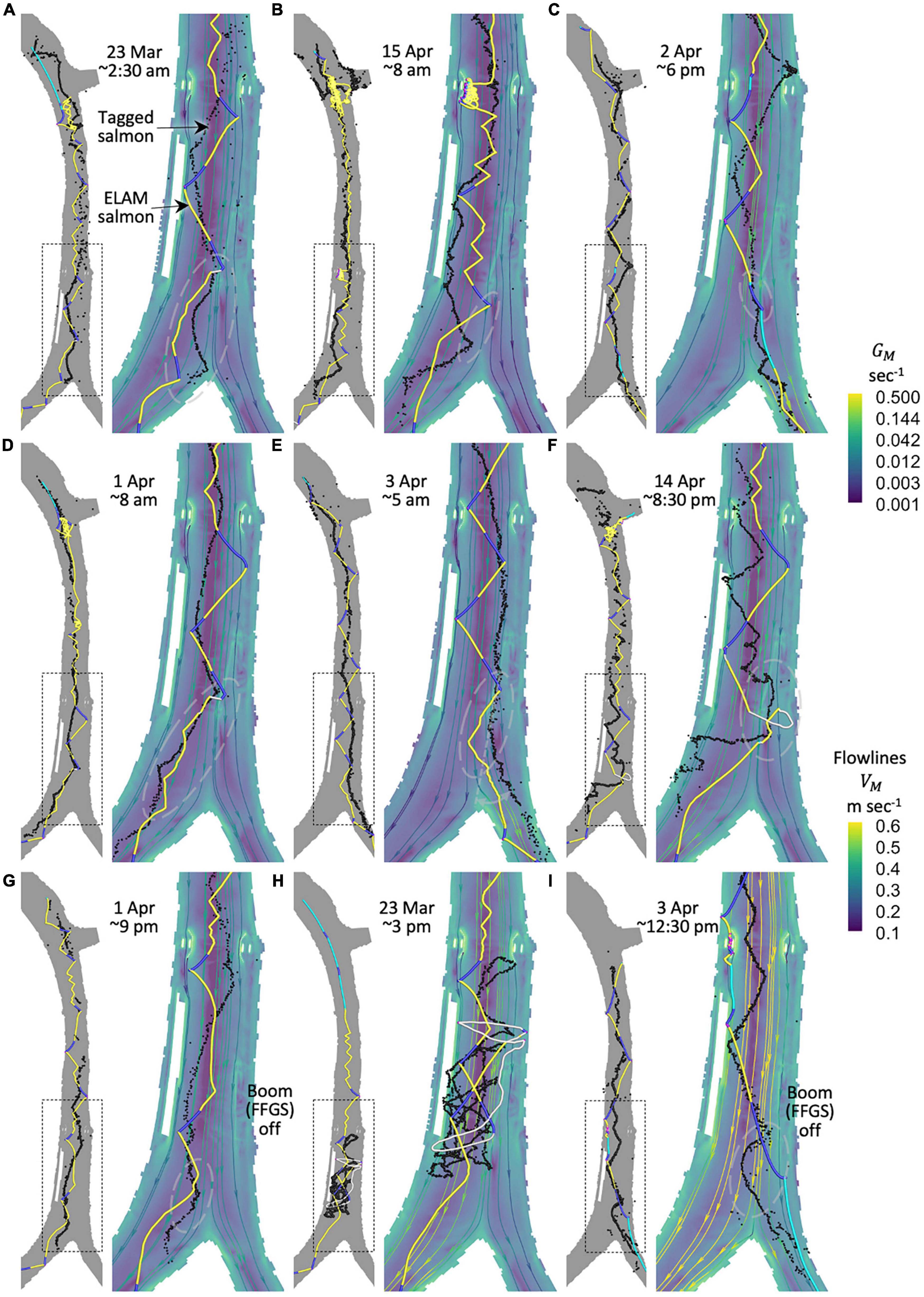
Figure 9. Year 2014 tagged and ELAM salmon response to the engineered surface guidance boom (FFGS) and the resulting entrainment. The ELAM model is built and calibrated with 2009 data, then applied without modification to year 2014 river conditions with the FFGS. Simulated salmon swim paths are responding to time-varying hydrodynamics at the same time that tagged fish are observed swimming through the river reach. Simulated salmon paths in the figure are included in Figure 8 heatmaps. Simulated salmon paths are colored by the behavior B (Tables 4, 5) and the tagged fish trajectory is colored black. Movement dynamics of simulated and tagged salmon near the FFGS are provided as dyads, where the left side is a zoomed-out view of the river reach and the right is a zoomed-in view of the FFGS with GM contoured as a fill color and river water flowlines colored separately. Each dyad (A–I) represents a different category of context-based salmon response to surface boom hydrodynamics. Additional details: the tagged salmon in panel (A) returns later and the one in panel (I) several days later. Paths in panel (B) illustrate a tagged and ELAM salmon that begin around midnight while the hydrodynamics are plotted for 8 am when the fish pass the FFGS and junction. In panel (E), we add a light gray geometric line and arc angle to ease visual interpretation of the tagged salmon direction before re-orientation toward Georgiana Slough. The tagged salmon path in panel (H) is longer than displayed and truncated here to ease visual comparison where primary similarities exist with the simulated fish.
We find that year 2014 simulated salmon swim paths in 2-D are not as heterogeneous as 3-D trajectories from year 2009. At least two factors are responsible. First, year 2014 lacks vertical heterogeneity. Second, horizontally, the 2-D depth-averaged hydrodynamic model output has a more diffuse laterally-distributed high-velocity core compared to the flow field rendered with an explicit 3-D flow field model (Figure 4). That is, in our 2-D flow field simulation, the higher velocity core is less concentrated in the river thalweg and distributed across a wider portion of the river’s width compared to 3-D rendering of the flow field. A 2-D representation of the river does not perfectly correspond with a particular depth from an explicit 3-D rendering of the flow field since 2-D and 3-D modeling assumptions are different. The more diffuse high-velocity core in 2-D flow field rendering has a concomitant impact on hydraulic derivatives, particularly GM. The impact of a more diffuse high-velocity core on GM results in wider cross-sectional excursions of the simulated fish. The greater amplitude of 2-D zig-zag paths can also be attributed to the physical domain of the river. Natural channel cross-sections are often u-shaped (Figure 5 upper left), so simulated salmon deeper will have less width (amplitude) before encountering hydrodynamics that trigger re-orientation compared to fish nearer the water surface where the river is widest.
Despite inherent tradeoffs involved with 2-D hydrodynamic simulation relative to 3-D, we can still use year 2014 outcomes to explain how salmon guidance and entrainment operates in the context of a salmon’s past hydrodynamic experiences integrated at multiple scales. The simulated salmon swim paths in Figure 9 are responding to time-varying hydrodynamics at the same time when tagged fish are observed swimming through the river reach. Simulated salmon paths in Figure 9 are included in the Figure 8 heatmaps. Simulated salmon perceptually sense and respond only to river hydrodynamics associated with the boom’s presence in the water flow field, that is, modeled fish do not physically interact with the FFGS structure rendered in the mesh and they can pass through to the other side by, conceptually, swimming under in 2-D.
We find that caution should be exercised when attributing observed salmon movement and entrainment to a surface guidance boom’s configuration and alignment. When the FFGS is deployed (on), hydrodynamics that emanate from the structure result in a filament of GM that starts at the boom downriver endpoint and extends to the riverbank apex at the junction point where the river bifurcates (Figure 9). Salmon initially deflected at the boom toward the Sacramento River can be subsequently attracted to the GM filament, drawing them toward Georgiana Slough (Figure 9A dashed gray region). However, not all boom encounters are followed subsequent attraction to the GM filament (Figure 9D dashed gray region). Salmon can be hydrodynamically deflected toward the Sacramento River at the boom (Figure 9A) and also by the GM filament downriver of the structure (Figure 9B dashed gray region). If the perceptual context is different, however, the filament can attract salmon into Georgiana Slough (Figure 9C dashed gray region).
Entry into Georgiana Slough is not always a result of filament attraction, as river flow can re-orient a salmon toward Georgiana Slough even if the salmon is initially deflected toward the Sacramento River (Figure 9E dashed gray region). Salmon can also respond to the boom by milling behind the structure (Figure 9F dashed gray region) or in front between the FFGS and dock on the opposite riverbank (Figure 9H dashed gray region).
River flow alone can direct salmon into the Sacramento River when the boom is not deployed (Figure 9G dashed gray region). Also, the GM filament exists in shorter form when the FFGS is off, extending upriver from the riverbank apex point of bifurcation. At times, the shortened filament can act in combination with GM emanating from the riverbank near the boom to attract salmon into Georgiana Slough even when it requires the fish to cross the critical streakline or water flowlines entering separate routes downriver (Figure 9I dashed gray region).
In summary, GM can both repulse, B{2}, and attract, B{3}, nearby salmon. Broadly, influence of the guidance boom on salmon depends on the context of the fish’s decision-making at the time of the boom encounter. Specifically, perceived hydrodynamic stimuli depend not only on the fish’s momentary sensing but also on its memories of past hydrodynamic experiences that are integrated at multiple scales.
Figure 10 summarizes all computational movements of simulated salmon. The increase in riverbank boundary interactions in 2-D (Figure 10) compared to 3-D and 2-D extractions of year 2009 hydrodynamics is a result of releasing simulated salmon where tagged fish are first detected. Some tagged fish show up for the first time at the riverbank where the geometric configuration of Eulerian mesh elements are complex because of wetting and drying. As the water surface rises and falls with river flow, mesh elements along the riverbank are identified as wet or dry by the 2-D hydrodynamic model. Since the ELAM model does not permit simulated fish to enter or cross dry mesh elements, the geometric configuration of wet elements at the river’s edge can, at times, be complex and in a practical sense trap some individuals from moving into the river toward the thalweg. Simulated fish that remain trapped along the riverbank for the duration of the simulation window in year 2014 show up in Figure 10 as mesh boundary encounters, but are otherwise not factored into our analyses. For instance, the trapped simulated individuals are treated as out-of-bounds releases and do not contribute to the swim path heatmaps.
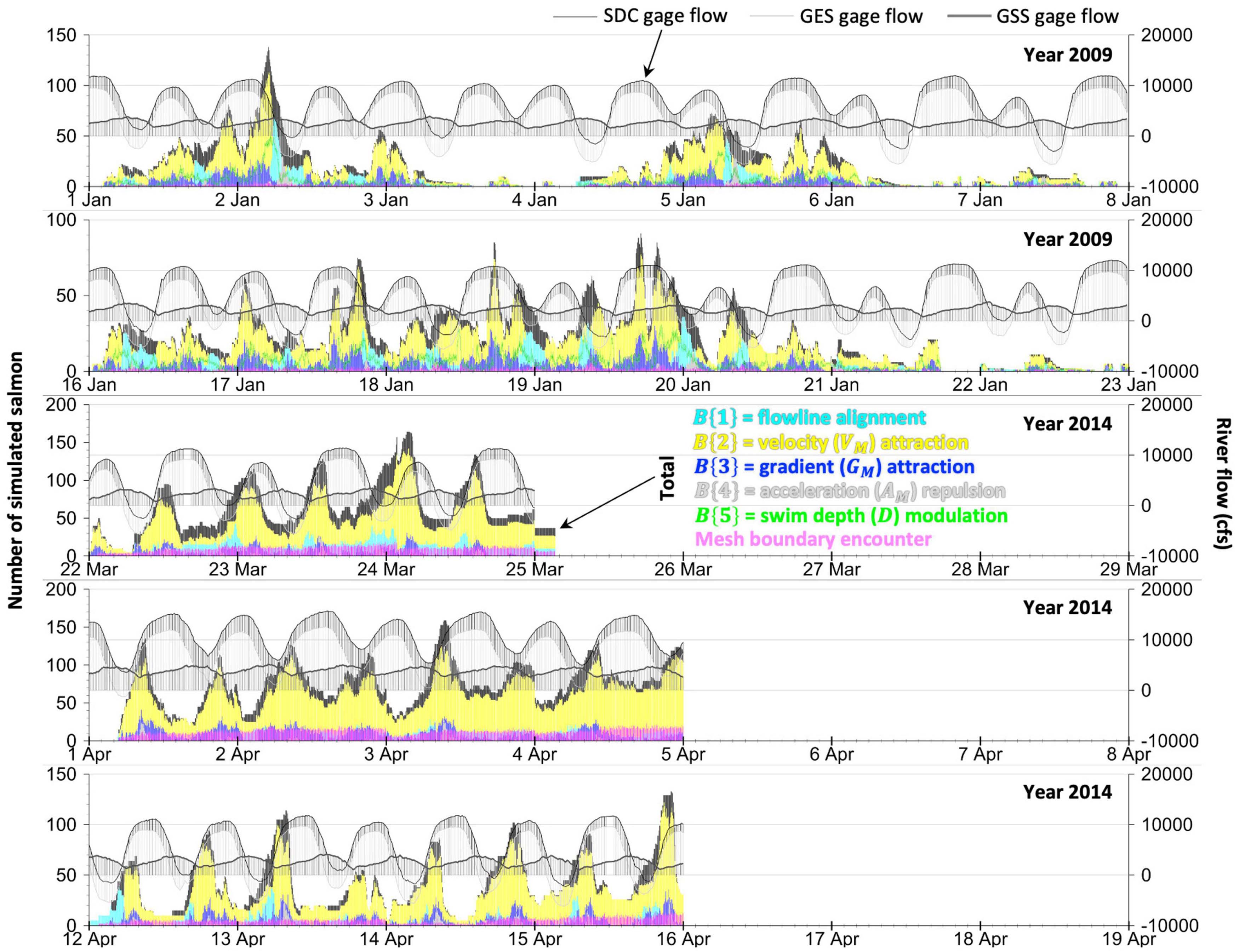
Figure 10. The distribution of behaviors B{1,2,3,4,5} over time within the simulated salmon population throughout the river reach that underlie the movement mode heatmaps (Figure 8), simulated salmon paths near the FFGS in year 2014 (Figure 9), and modeled entrainment (Figure 11). The sum total of simulated salmon making decisions within the ELAM model domain at any given time (black) is decomposed into the number implementing each constituent behavior. Behavior proportions are overlaid, not stacked, with behaviors least represented in the population plotted overtop more predominant responses. Note how flow hydrodynamics as viewed by the gage stations (Figures 1, 2) change temporally and also by location within the river reach. Simulated salmon behaviors are updated every 2s in response to river hydrodynamics that update at 3−min intervals. Note that B{5} is a vertical-only response that occurs simultaneously together with an xy-plane orientation set by one of the following behaviors from B{1,2,3,4} and can only be implemented in the year 2009 3-D mesh.
4.2. Passage/entrainment
The model performs well in the quantitative performance metric of greatest interest to our study, passage/entrainment (Figure 11). Final passage/entrainment is the permanent, final exit of individuals into either Georgiana Slough or the Sacramento River downriver of the junction (Figure 8). Root-mean-square error (RMSE) is a simple yet robust metric that quantifies the difference in the final passage percentages (i.e., ultimate measured fate or entrainment) between the tagged and simulated salmon across 7−day contiguous multi-day windows for year 2009 and 3− and 4−day contiguous windows for year 2014. The ELAM model generally reproduces past and predicts the near-future passage/entrainment with an RMSE ≤ 10 (Figure 11).
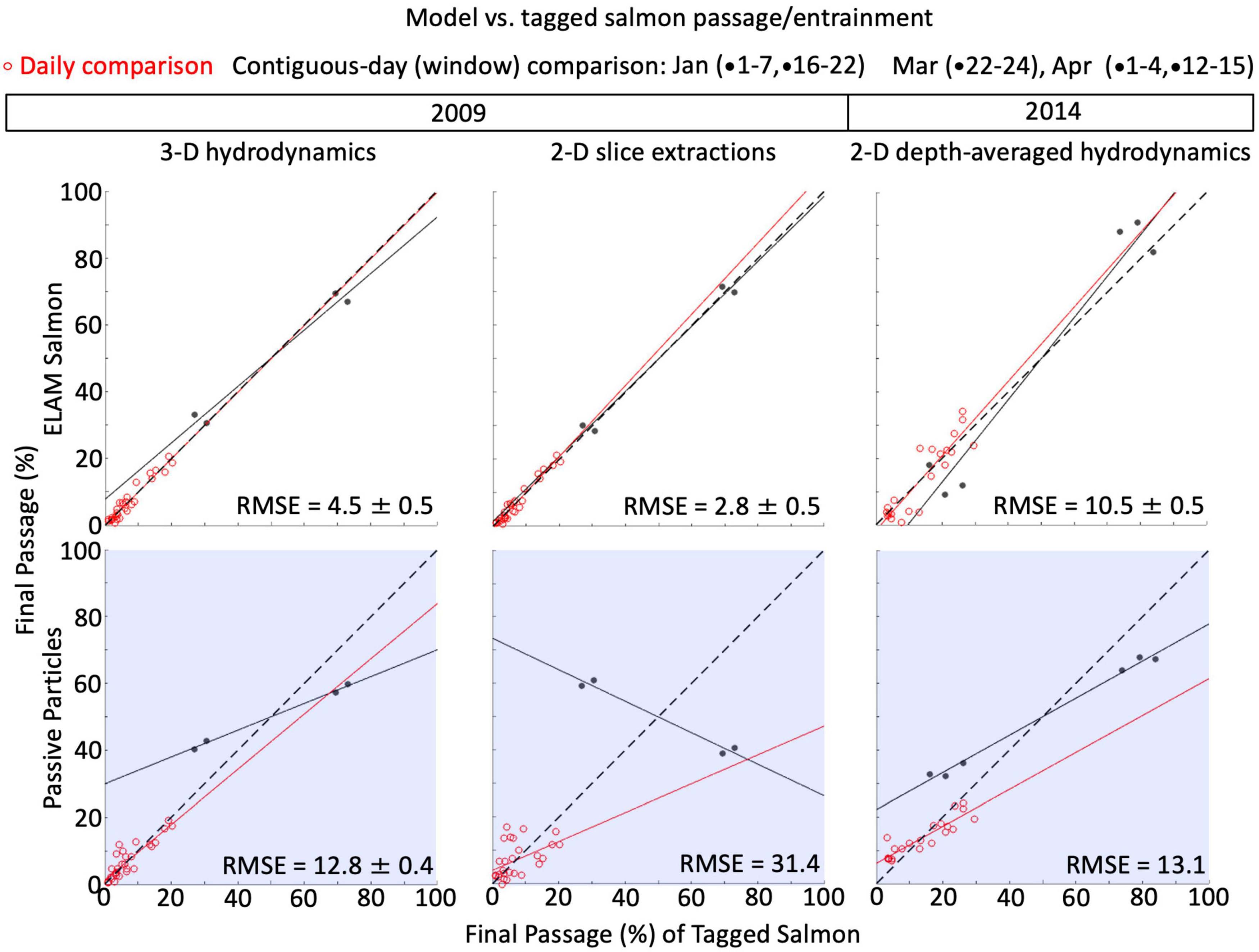
Figure 11. Comparison of tagged versus modeled salmon passage/entrainment. The ELAM model is developed with year 2009 data (left and middle panels), then applied without modification to out-of-sample, year 2014, river conditions that include a surface-oriented boom for guiding salmon (right panels). Passive particle passage/entrainment is plotted with a blue shade background. Each dot represents a comparison of tagged salmon versus simulated individual (fish or particle) passage/entrainment on a percentage basis (%) downriver into either Georgiana Slough or the Sacramento River. There is one dot for the Georgiana Slough proportion and one for the Sacramento River. There are two black dots (Georgiana, Sacramento) for each simulation window (Figure 2), which represent the total cumulative passage/entrainment; for instance, in year 2009, there are two black dots for the cumulative passage during 1–7 January and another two black dots representing the total entrainment across 16–22 January, resulting in four total black dots. Red dots are smaller in magnitude because they represent the daily portion of the total (window) percent that went downriver in each route. The root-mean-square error (RMSE) is based on the cumulative passage/entrainment on a simulation window basis, i.e., the black dots. No 3-D model is used for year 2014; instead, a 2-D depth-averaged model is used to render year 2014 river hydrodynamics with the surface guidance boom.
We run sensitivity analyses to evaluate some key uncertainties in the model and its intended future use. Specifically, the standard deviation following the ± symbol (Figure 11) is generated by varying the random number generator seed that is part of the algorithm ensemble (Table 6) and, for 3-D, we also vary the random guesses of the release depth (z-coordinate).
Simulated salmon and passive particles that make up the passage/entrainment proportions are responding to time-varying hydrodynamics, and the classified movement modes of all these modeled individuals are heatmapped (Figure 8). A temporal distribution of behaviors (Figure 10) throughout the river reach underlies resultant passage/entrainment (Figure 11). No single hydrodynamically-mediated response behavior is solely responsible for the passage/entrainment pattern at the junction.
Passive particle passage/entrainment (Figure 11 blue shade background) represents neutrally-buoyant individual movement when the perceptual decision-making behavior is turned off. Passive particles are analogous to an entity merely following the flow/flowlines.
4.3. 3-D vs. 2-D
In 2-D simulations, both the vertical z-coordinate (depth-oriented) hydrodynamics and fish swim orientation/speed are eliminated. In the 2-D slice extractions for year 2009, a 2-D xy-plane horizontal slice is extracted from just under the water surface for each output in the original 3-D flow field time series. Simulated salmon passage/entrainment is resilient to the simpler 2-D descriptions of the river (Figure 11). Also, we provide an example comparison of a 3-D swim path (Supplementary Figure 1) and its 2-D counterpart within an extracted slice of the same hydrodynamic condition (Supplementary Figure 2).
The 3-D vs. 2-D passage/entrainment outcome suggests that the analysis of salmon with modeled perceptual decision-making may not always require the maximum permissible hydrodynamic resolution. Elimination of the vertical hydrodynamics and swim orientation/speed alone does not appreciably change the simulated salmon entrainment or trajectories, e.g., comparing Supplementary Figures 1 vs. 2, in our relatively shallow system domain. Nonetheless, modeling hydrodynamics as depth-averaged in lieu of 3-D phenomena does appear to influence the character of year 2014 swim path cross-sectional excursions compared to those in year 2009 regardless of whether the simulated salmon movement is generated from 3-D or 2-D slice representations of the water flow field.
4.4. When salmon entry pattern is unknown
Future predictions of fish movement behavior for informing water operations engineering and management do not always have the benefit of knowing how salmon will enter the domain of interest. We revisit year 2009 and 2014 passage/entrainment results without the benefit of tagged salmon to inform the release of simulated individuals (fish and passive particles) and with the added simplification that B{4} is a cruise speed response regardless of the river flow field. The B{4} simplification stems from more recent continuing efforts to simplify the model wherever possible, finding that the parsimony has an undetectable impact on simulated passage/entrainment.
While one can discount the timing of releases in steady (unchanging with time) hydrodynamics, e.g., Smith et al. (2010), when the environment itself varies with time then both the time sequencing and spatial distribution of individual entries into the domain could impact model outcome. To release simulated fish and passive particles into the domain without the aid of tagged salmon data, we arbitrarily use three different quantities of individuals per 24-h period, three spatial configurations (i.e., point, normal, log-normal distributions), and up to twelve different time intervals (Figure 12). Spatially, we release all simulated individuals within the same cross-sectional transect located at “abc” (Figure 8). Temporally, we release individuals separately and in clusters (Figure 12 upper right). Simulated individuals are released irrespective of the river flow condition at the moment of release.
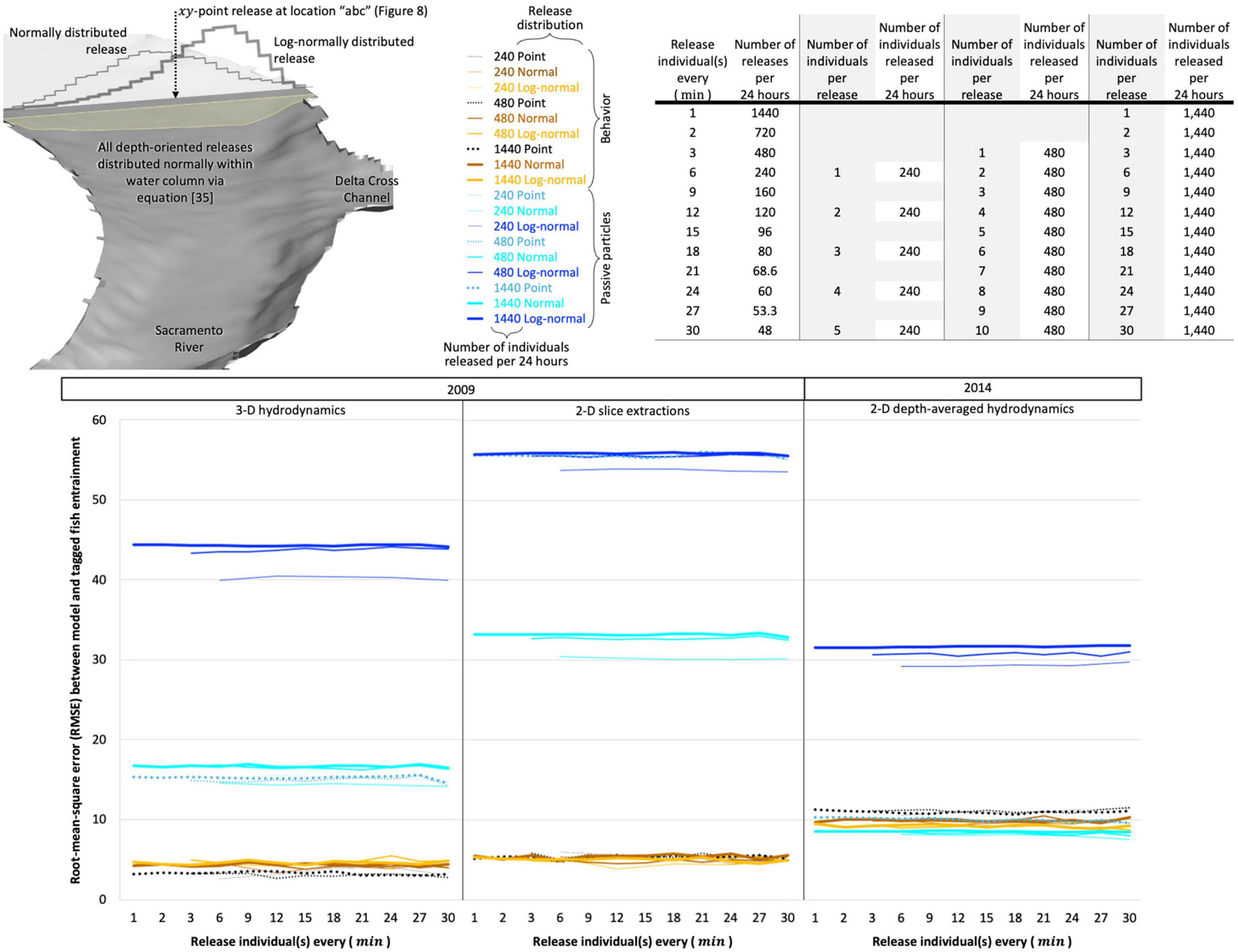
Figure 12. Modeled passage/entrainment without the benefit of tagged salmon to inform the release of simulated individuals. Simulated individuals (fish and passive particles) are released using three different quantities per 24-h period, three spatial distributions (point, normal, log-normal) and, in time, up to twelve different ways (upper right). All simulated individuals are released within the same cross-sectional transect located at “abc” (upper left). Model accuracy in the form of root-mean-square error (RMSE) for each release alternative is plotted separately using a unique line and color combination (upper middle). The RMSE of simulated fish passage/entrainment relative to tagged salmon is plotted using black or shades of orange while passive particles use shades of blue (upper middle). RMSE quantifies the difference in final exit passage/entrainment proportions (ultimate measured fate) between tagged salmon and simulated individuals (bottom half).
We plot the results of the sensitivity analysis in the form of root-mean-square error (RMSE) of the release alternative outcomes. The RMSE quantifies the difference in final exit passage/entrainment proportions (ultimate measured fate) between tagged salmon and the simulated individuals. A result is not plotted if the number of permanent exits downriver is less than 75% of the total attempted releases, which occurs only in two instances: point releases of 1, 440 passive particles in the year 2009 3-D domain when released at intervals of 6 and 21min apart.
Simulated fish passage/entrainment is resilient to alternative releases when RMSE is based on a contiguous passage/entrainment fate integrated over multiple days: 7−day windows for year 2009 and 3− and 4−day windows for year 2014 — the same method in Figure 11. Passive particles can resemble the passage/entrainment during 2014 hydrologic conditions when released using a point or normal spatial distribution, but log-normally distributed passive particles biased toward the outside bend of the river perform poorly for both year 2014 and 2009.
5. Discussion
We describe a cognitive approach to the mechanistic modeling of fish behavior responses to river hydrodynamics at the scale that water operations infrastructure is designed and managed. The ELAM model quantitatively describes and reproduces selective tidal stream transport patterns of downstream-migrating juvenile Pacific salmonids and predicts their guidance and passage/entrainment patterns in out-of-sample data across diverse environmental contexts. We find that a mix of behaviors (Figure 10) underlies our modeled swim paths (Figure 8) and passage/entrainment outcomes (Figure 11).
Our theoretical approach suggests that a behavioral mix is most likely to emerge in regions dominated by nonacute stimuli. ELAM analysis helps conceptualize the nuanced influence that engineered structures have on the movement of downstream-migrating salmon (Table 5: Engineering design relevance). The intended use of the ELAM model is to inform how future fish passage/entrainment outcomes may result from water operations infrastructure management and design. A numerical behavior model in which simulated fish quantitatively reproduce observed, tagged salmon passage/entrainment patterns (Figure 11) aligns with the tool’s intended purpose.
Reproducing past animal movement patterns (hindcasting) is one way to establish confidence in a model’s validity (Getz et al., 2018; Leitch et al., 2021). A model’s accuracy should stem from the underlying mechanisms, and comparing quantitative predictions to new observational data is one of the strongest tests of scientific theory (Dietze et al., 2018).
Our goal at the outset of the study was to develop a decision-support tool capable of quantitatively reproducing passage/entrainment proportions within an arbitrary root-mean-square error (RMSE) of approximately ten, similar to previous work in other environmental contexts (Goodwin et al., 2006, 2014). In this system, ELAM model accuracy visibly degrades as RMSE exceeds approximately twelve (Figure 11) and RMSE much below ten has diminishing benefit.
A key finding of our work is that the repertoire of hydrodynamic responses in a tidal setting are theoretically consistent with — a superset of — the behaviors that juvenile Pacific salmonids exhibit in simpler, steady flow reservoir settings (Figure 13). Salmon often navigate both reservoirs and dams in the upper watershed (Martinez et al., 2021) followed by tidal environments closer to their ocean entry. The ability to mathematically describe, reproduce, and predict fish movement behavior across such diverse environments strengthens water operations decision-support in application to scenarios outside the range of conditions to which the tool is calibrated, a typical need of engineering and management design future forecasting.
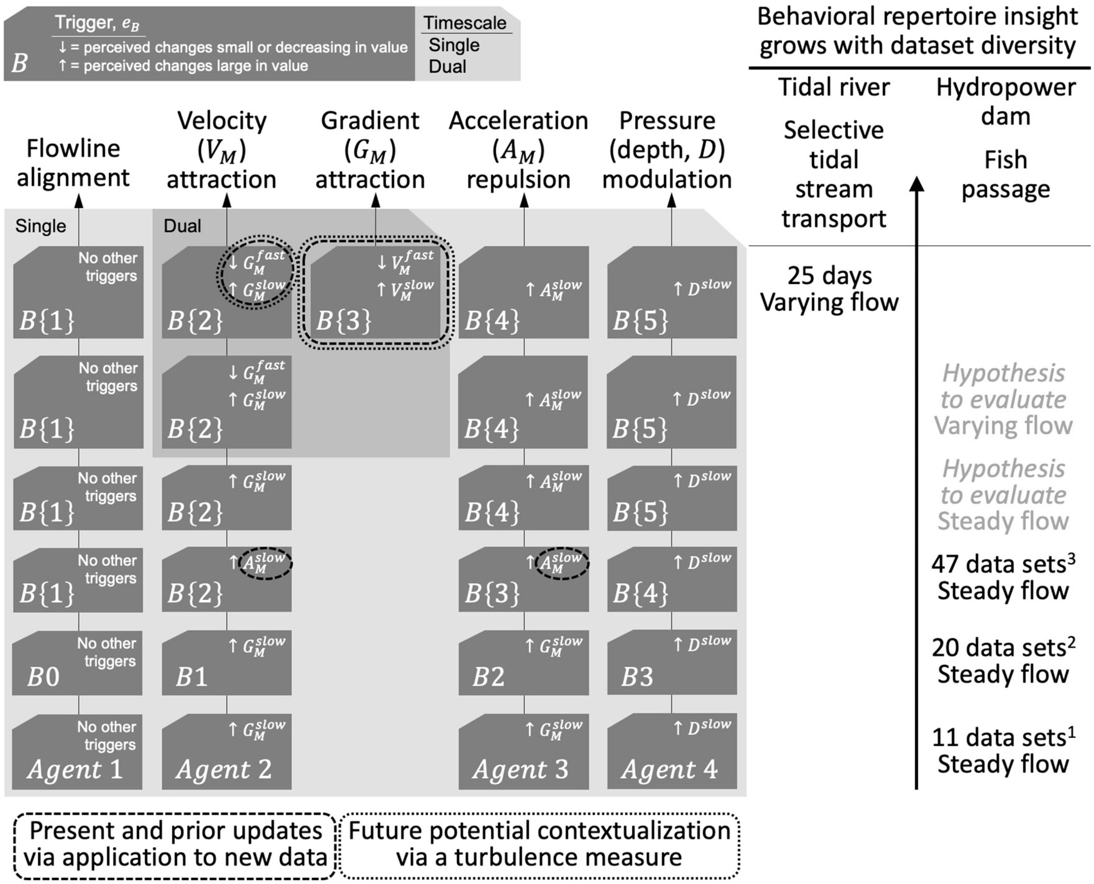
Figure 13. Results to date and future potential improvements from iterative near-term ecological forecasting (Dietze et al., 2018) in the context of fish passage, guidance, and movement prediction for water operations management and infrastructure design. The salmon movement behavioral repertoire developed in our tidal study is a conceptual superset of the fish hydrodynamic responses found in simpler environments represented with steady flow. Old notation from past applications: to a single dam 1Lower Granite Dam (Goodwin, 2004), 2multiple dams (Goodwin et al., 2006), and 3basin-wide (Goodwin et al., 2014) where GM and the term strain in prior works1,2 are interchangeable for the data and acclimatization is used1,2 instead of the terms habituation and memory used herein.
The model herein is an abstraction of reality and the underlying mechanics are not a holistic description of salmon movement behavior or the cognitive architecture of fish. There is no such thing as a perfect ecological forecast (Dietze et al., 2018). Numerous questions remain for future study. In the model’s minutiae, for instance, we identify at least two instances where practical functionality deviates from anticipated theory. First, E4 differs from the nsd construct of other stimuli, Equation 20 vs. 2; that is, our current formulation for describing perceived changes in intensity does not appear to work as anticipated when using depth as a proxy for salmon swim bladder pressure. Second, outperforms I2 in from Equation 24; that is, we find that I2 in does not work and that Equation 24 is the construct that works within our modeling approach for an immersed individual to perceive meaningful large spatiotemporal scale changes in river water speed due to the tides. Perhaps the deviations are the result of simulated abstraction and limited mensuration of the real world.
At a broader level, our work raises the question of how many timescales animals may use and how the number might be related to environmental and social complexity (Rodriguez-Santiago et al., 2022; Tump et al., 2022; Li et al., 2023). Our work provides a basis upon which further improvement and advancement is likely. Further improvement must confront nontrivial tradeoffs that we discuss next.
5.1. Model realism vs. usefulness
The ELAM is similar to other models in that it is a simple, finite, and abstract representation of reality. Perhaps the single biggest challenge of our work is finding the best balance between model realism and usefulness in the context of how the tool is to be used. Tradeoffs between model realism and complexity are a common problem (Getz et al., 2018). Increasing model complexity can come at the expense of concomitant deleterious impacts on tool transferability to settings beyond which the tool is calibrated (Yates et al., 2018).
Realism can be added in the form of more detailed hydrodynamics and/or behavior rules. The practical downside of increasing the model’s complexity for realism alone is the additional computational burden incurred, which then reduces the resources available to explore and improve the model elsewhere. Determining the most important real-world features for a model to reproduce is paramount, yet rarely straightforward. The demands of scientific inquiry and engineering construction deadlines are rarely in perfect synchrony.
Hydrodynamic modeling impacts the realism of simulated trajectories. Additional flow field heterogeneity and stochasticity provided by DES or LES compared to RANS (Figure 4) would likely result in more heterogeneous, and thus realistic, simulated trajectories. As is, our modeled salmon entrainment predictions (Figure 11) are generally insensitive to vertical hydrodynamics and vertically-aligned movement behavior B{5} in the relatively shallow Sacramento River. Nonetheless, secondary currents (Dinehart and Burau, 2005; Fong et al., 2009; Constantinescu et al., 2011a; Moradi et al., 2019; Yan et al., 2020; Schreiner et al., 2023) and water column heterogeneity should not be entirely discounted as a factor in salmon entrainment (Ramón et al., 2018). Selective tidal stream transport (Creutzberg, 1961) may be driven by multiple factors (Benson et al., 2021; Gross et al., 2021b) including vertically-aligned hydrostatic pressure (Tielmann et al., 2015) and horizontal, cross-sectional gradients in water turbidity (Bennett and Burau, 2015).
Adding explicit behavioral variation to our simulations through distributions of animal characteristics, such as size or orientation tendencies (movement modes), would likely improve the realism of simulated trajectories. Presently, we eliminate (zero-out) all permissible stochasticity and heterogeneity not explicitly required to meet our primary objective — reproduce and predict future passage/entrainment — in order to minimize the number of tunable parameters. We find that discerning meaningful parameter influences on key mechanics of the model is far more challenging when other forms of variability (stochasticity) are present in the model, e.g., attributes with the sole purpose of increasing the “wiggle” realism in simulated fish trajectories. While discerning parameter influence on model performance amid stochasticity is a challenge that can be met with Monte Carlo or similar methods, again, increasing the computational burden within a study has tradeoffs with those resources becoming unavailable elsewhere where they might have a greater overall impact. ELAM model parameter values herein do not change during simulation and are identical across all the analyses described, the only exception being the random number seed varied for computing the standard deviations in modeled entrainment (Figure 11).
There are many opportunities for future improvement relevant to the data presented herein and in application to other systems. For example, alternative algorithms exist for every ensemble constituent (Table 6). Continuing work can improve our understanding of fish and the mechanics required to meet fish passage research and water operations goals, just as this work builds upon previous work (Figure 13 and Tables 1, 3). In the next section, we discuss some of the more noticeable aspects of our modeling approach, shortcomings, limitations, and future improvement opportunities.
5.2. Fish swim paths
Simulated salmon paths emerge from behaviors that depend on past experience, resulting in movement trajectories that differ among individuals experiencing the same momentary condition. In our approach, two hypothetical fish experiencing the same condition at a moment in time will exhibit different behaviors and, therefore, movement paths because their past histories are not identical.
While examples can be found in our study in which two simulated salmon — or a simulated and tagged fish — trace nearly the same path (e.g., Figures 8, 9), more generally, pairs of individuals (modeled versus modeled; modeled versus tagged) do not have identical trajectories that coincide both spatially and temporally. Thus, our study highlights a surprising but useful paradox: that is, one-to-one paired synchrony between simulated and tagged salmon paths, while desirable, is not a requisite for satisfactory hindcasting and future prediction of route passage/entrainment. Upon inspection, there are several reasons for the paradox.
One reason for the paradox is that movement dynamics near the junction are more important for determining entrainment than behavior elsewhere within the river reach. Therefore, paths do not have to coincide perfectly both spatially and temporally throughout the entire reach. The most important factors for the correspondence between modeled and tagged fish passage/entrainment proportions in our tidal study are that each of the sample populations (i) volitionally control much of their displacement and fate within the river channel, in contrast to passive particles, and (ii) make decisions similarly-enough in similar-enough proportions across a broad range of conditions. Location holding is one way that a tagged salmon may sample river hydrodynamics analogous to a simulated salmon, but at a later time after milling in a region for a while. Another reason for the paradox is that the sample sizes, while somewhat relatively small once parsed to our simulation windows (Figure 3 upper left), are sufficient to average out a variety of characteristics both in salmon movement and in experienced water flow patterns as evidenced by the sensitivity analysis (Figure 12).
5.2.1. Movement mode heatmaps
We use heatmaps to compare swim path patterns and movement modes across our samples of virtual and real fish. The relatively concentrated simulated salmon swim paths along the river thalweg (Figure 8), compared to tagged fish (Figure 3), can likely be improved by distributing the modeled fish further throughout (across) the river’s width by increasing the presently-negligible stochasticity in swim orientation. Increasing swim orientation stochasticity, however, will come at the expense of slowing down their speed-over-ground that is already slower than tagged fish. Speed-over-ground could be increased by implementing faster swim velocities (e.g., larger fish), but bigger individuals will bias the decision-support tool away from resembling the smaller-sized salmon important to water operations management. A distribution of small-to-large salmon fork lengths is likely a desired next step, but not part of the study herein.
Another possibility for reducing the discrepancy between simulated and tagged salmon path concentrations is modifying how the sensitivity of perceived changes in GM and VM are handled. Presently, GM and VM perceived changes are handled via threshold values that do not change with time. Perhaps the threshold values, instead, depend on previous hydrodynamic experience, which would add yet another layer of contextuality to behavior.
Further, the GM trigger and attraction behavior may themselves be contextualized via multimodal signal integration (Gil-Guevara et al., 2022) with a turbulence measure (Figure 13). While our development efforts with year 2009 data reveal that TKE is sometimes not present in areas where salmon repeatedly re-orient (Figure 6 and Supplementary Figures 1, 3, 5), perhaps the less pronounced TKE values have value in eliciting less concentrated paths when used in combination with our existing hydrodynamic triggers (Table 5). A challenge within the above endeavor is to realize a more distributed concentration of simulated salmon swim paths across the river’s width without incurring a concomitant increase in boundary interactions.
Other observed discrepancies between simulated and tagged salmon evident from the heatmaps (Figure 3 vs. Figure 8) include more tagged salmon exhibiting reach milling and riverbank tendencies, although this is a natural byproduct of our focus on zig-zagging behavior. Interestingly, heatmaps reveal similarities between tagged and simulation salmon milling near the bridge despite the piers (and associated hydrodynamics) being absent from the year 2009 flow field renderings.
5.2.2. Synchronizing modeled and tagged fish swim paths
A better end-state of the model would preserve the existing entrainment fidelity while gaining full synchronization between real and simulated fish trajectories (path plus timing), which requires reproducing the emergence of different movement modes in the same proportions. Manual classification was best able to handle anomalies in the real-world fish data for this present study, but future work should focus on automated methods that can assist the development and parameterization of more realistic reproductions of tagged fish movement modes and individual trajectories.
A solid next step would be a quantitatively rigorous movement mode classification (Romine et al., 2014; Vilk et al., 2022) combined with trajectory similarity measures such as the Fréchet distance or dynamic time warping (Magdy et al., 2015; Cleasby et al., 2019; Su et al., 2020; Tao et al., 2021) for gauging the one-to-one correspondence between pairs of simulated and tagged salmon swim paths. Larger (longer) river spatial domains and temporal windows would facilitate the analysis of movement mode emergence, allowing us to better understand whether modes are more closely correlated with specific individuals, a particular sequence of environmental experiences, or a mix of factors.
Existing travel time discrepancies between simulated and real fish may be improved through the previously mentioned tactic of releasing modeled salmon with a distribution of sizes (fork lengths). Larger fish swim faster if the assumed bodylengthspersecond remains unchanged, although it is also possible to modify the assumptions of drift, cruise, and burst swimming BL s−1 for our identically-sized 120 mm salmon. With the model as is, we discuss three possible explanations for the slower transit time of the simulated salmon example in ebb flow (Figure 8 and Supplementary Figures 1, 2): swimming depth, rheotaxis, and RANS flow field modeling, all of which relate to hydrodynamic model fidelity that we discuss in the next section.
5.2.3. Hydrodynamic model fidelity
Rivers have more heterogeneity than we can fully measure or model (Figure 4), and the issue is relevant to fish movement analysis as evident in the comparison of real and simulated travel times in Figure 8 and Supplementary Figures 1, 2 during ebb flow. Our fish behavior simulations using 2-D xy-plane horizontal slices use the hydrodynamics extracted from just under the water surface where river flow is typically fastest (Supplementary Figure 2). In 2-D, simulated individuals cannot move along the river bottom where water speed is slower and sometimes approaches zero. Given that 2-D simulated fish transit times (Supplementary Figure 2 particle: 46min; salmon: 1h 1min) are similar to the results from 3-D (Figure 8 and Supplementary Figure 1 particle: 46min; salmon: 1h 3min), we can conclude that vertical heterogeneity in river flow contributes negligibly to the travel time of these specific individuals over the duration they journey the reach in this flow condition.
Notice that the tagged fish transits the stretch in 41min while the passive particle takes 46min. The result appears at first inconsistent with our finding that simulated salmon must orient against the flow, which slows ELAM fish relative to a passive particle. Orienting the simulated 120mm sized salmon more with the flow (negative rheotaxis), however, increases the zig-zag period (wavelength) that reduces similarity between simulated and tagged fish swim paths.
Another possible explanation for the longer simulated salmon transit time resides in the notion that RANS modeling represents an average flow field condition of the river (Figure 4). RANS flow field modeling can miss high-velocity regions or cores (Constantinescu et al., 2011b). We surmise that real-world flow field heterogeneity provides tagged salmon opportunities in the real world to exploit regions of faster-than-RANS water that is unavailable to simulated fish and may at least partially explain the slower transit times of the modeled fish in ebb flow (Figure 8 and Supplementary Figures 1, 2).
5.2.4. Behavioral choice/decision model fidelity
Mathematical models of decision choice, and the dynamics that underlie them, are an active area of research not only in ecology and ethology but other fields as well, especially the field of economics, and have been for more than a half-century (Table 1). There are many different choice/decision models to choose from. The scale of our study and the assumptions we invoke do not make our study or findings the best platform to advocate for one theoretical approach (theory, model) over another. Others may find in work at the same scale (but different environmental context) or at different scales (the laboratory) that there are advantages/disadvantages to a particular theoretical approach which differ from our experience here. In this study, using sensory evidence accumulators at our available scale, we find that for the rise and fall of competing behaviors in the hierarchical repertoire to generate the type of fast response dynamics we observe in tagged fish in particular areas (e.g., near the riverbank) that we need the contribution of inhibition in our decision model. In our approach, inhibition facilitates a better transition between behaviors B{2, 3} by keeping their sensory accumulators, eB (Equations 4–7), in a more stable harmony compared to the same formulation without inhibition. Without inhibition, we find that B{2, 3} responses in some contexts are simply too slow to resolve themselves when needed because the impending behavior must catch-up and overtake the accumulated evidence of another behavior’s eB and by the time the former outraces the latter the simulated fish encounters a boundary, is captured, or is entrained, for instance.
5.3. Fish passage/entrainment
Synchronizing real and simulated worlds in order to compare salmon passage/entrainment proportions is not straightforward. Tagged salmon may occupy the river reach domain prior to our simulation window and/or remain in the area afterward (Figure 8), which limits the number of tagged salmon that we can leverage in short windows. Analyzing the entire 2008–2009 and 2014 field seasons (Figure 2) with larger spatial domains extending upriver and downriver would allow us to piece apart further nuances of salmon movement modes, as previously mentioned, as well as incorporate more of the available fish field data. ELAM applications that far exceed previous limitations are becoming viable with hardware improvements (Rodi, 2017) and the ability to work with trillion-cell hydrodynamic solutions on a common computer (Imlay et al., 2018).
5.3.1. Release distribution
Decoupling the cognitive algorithm ensemble from a realistic entry of fish into the river reach domain results in simulated individuals that cannot sample the environment perfectly in line with tagged salmon. We can use alternative release distributions to assess the model’s prediction performance in the context of an unknown future, but in which post-construction monitoring may provide data on how real fish responded to the management action. We measure model accuracy using RMSE based on multi-day contiguous windows (Figures 11, 12). Daily passage/entrainment numbers are inherently more variable due to the fewer available numbers of tagged salmon (Table 2) and simulated fish that make up the proportions. There is value in integrating field and model passage/entrainment data over multiple days.
5.4. Guiding fish swim paths with surface booms and engineered hydrodynamics
Fish guidance is a major focus of water operations management and engineering in many rivers worldwide. Fish guidance has been attributed to turbulence plumes (Coutant, 1998, 2001; Zielinski et al., 2021) and also to velocity VM attraction triggered by a stimulus (Goodwin et al., 2006, 2014). The VM attraction hypothesis of fish guidance assumes the two hypotheses are compatible as turbulence is correlated in many settings with GM and AM identified as trigger proxies (Figure 13).
Analyses of fish guidance along surface booms using 3-D hydrodynamic modeling that led to the VM attraction hypothesis have yielded different triggers, and the exact trigger remains unclear. Initial studies using the VM hypothesis attributed the trigger to GM only for later analysis to suggest AM (Figure 13). Our study here advances past contradictions toward a consistent explanation worth evaluating further; that is, GM and AM play different roles near guidance structures. Here, we find that GM triggers VM attraction along booms which corroborates some findings in laboratory experiments (Swanson et al., 2020). Acceleration AM on the other hand acts to repulse salmon.
A topic for future research is whether GM attraction (triggered by VM) acts in combination with VM attraction (triggered by GM) to elicit salmon guidance along infrastructure and, if so, the relative contribution of GM attraction. Also worthy of further investigation, as mentioned previously, is how turbulence may act in combination with GM and VM as a trigger. Regarding acceleration, our findings add to the body of evidence that AM can repulse fish (Haro et al., 1998; Kemp et al., 2005; Enders et al., 2009a,2012; Vowles et al., 2014).
5.5. Other behavioral stimuli — temperature, dissolved gases, sound, and bubbles
Many of the concepts and theory that we leverage do not originate from studies on fish or hydrodynamics. Therefore, our approach may be extendable in aquatic systems to other environmental variables (Table 1). Insonified bubble curtains with light stimuli were deployed at the Sacramento River junction with Georgiana Slough in years 2011 and 2012 (California Department of Water Resources, 2012, 2013; Perry et al., 2014) and remain a future management option in the Bay-Delta to improve system-wide salmon survival.
5.6. Engineering best practices for predicting fish response to water operations
To facilitate iterative near-term ecological forecasting (Dietze et al., 2018) that can support water operations infrastructure engineering and management, we need best practices. We can begin developing engineering best practices for using fish movement simulations to inform civil infrastructure design and water operations management in the context of future environmental conditions that cannot be fully known in advance. While fish in the future observed during post-action monitoring are likely to experience hydrodynamics that differ in some ways from the assumptions in management design, there are several ways to maximize the utility of fish movement prediction given inherent and unavoidable limitations.
The first way to maximize the utility of fish movement prediction in design is to simulate their response to alternative designs, with each engineering concept evaluated across numerous future environmental conditions. Best practice would be to simulate across, or bracket, the likely future environmental conditions. Unfortunately, the drawback of the first method is the large number of simulations that can quickly outrace available resources.
The second method compares future design alternatives only in the context of the same conditions as past observations. The benefit of the second method is that past observations can inform some of the model’s initial conditions, e.g., fish entry patterns, and simulated future outcomes can be benchmarked relative to historical data in the null case of zero changes. The downside of the second method is the limitation of the design analysis to only past observed conditions that may not be relevant to the future.
The third method compares the performance of alternative design concepts relative to one another, with no relation back to past observed historical patterns. The benefit of the third method is that the analysis of future designs can use environmental conditions that differ from the past and fewer contexts (simulations) are needed for a trend to emerge that may identify a particular design as most robust across diverse environmental states. The downside of the third approach is that at least two design alternatives are needed to make a minimal, relative comparison.
5.7. Real-time fish prediction with theory-informed machine learning
Emerging new forms of automation can help address existing ELAM model shortcomings. Easier and faster implementation of the ELAM is needed to scale-up our approach for informing water operations management and design. We are working to encode our cognitive approach, such as multiplex signal disentanglement via multi-timescale perceptions, into a reduced-order form using theory-informed neural networks. The potential is motivated by the recent revolution of physics-informed neural networks (Karniadakis et al., 2021), reinforcement learning (Reddy et al., 2018; Ullman, 2019; Gunnarson et al., 2021; Li L. et al., 2021; Zhu Y. et al., 2021), and emerging concepts for improving machine learning by constraining them with psychological theory (Bhatia and He, 2021; Peterson et al., 2021). A reduced-order form of the ensemble algorithms in our approach may work better for the tight schedules that are common in engineering design projects. Machine learning has the potential to improve cognitive modeling by circumventing complicated assumptions about perception, attention, and memory that burden many existing methods (Bhatia and He, 2021; Peterson et al., 2021).
At the same time, hydrodynamic RANS, DES, and LES models will only grow in capability. As 3-D modeling of rivers becomes more sophisticated, cognitive-based approaches to mechanistic and machine learning based fish prediction may find particular value in new, in situ measurement technologies such as Infrared Quantitative Image Velocimetry or IR-QIV (Schweitzer and Cowen, 2021). River-wide, centimeter-scale IR-QIV hydrodynamic measurements can not only inform hydrodynamic modeling but also, paired with biologgers measuring fish orientation and swim speed, provide the real-time data streams needed to inform on-the-fly ELAM theory-informed machine learning. On-the-fly ELAM theory-informed machine learning has potential to provide real-time fish prediction of behavioral response, whether seconds or days in advance, greatly reducing the present time it takes to implement an ELAM prediction analysis.
5.8. Ethohydraulics with environmental modeling to improve waterways engineering
Recursively applying near-term predictions of fish movement followed by later comparison with observed data improves ecological research relevance to society by informing sustainable decision-making (Johnson et al., 2020) and accelerating the pace of scientific discovery (Dietze et al., 2018). Our present approach to behavior modeling is an outcome of iterative, trial-and-error work (Figure 13) to account for fish cognition in the interpretation and near-future prediction of their movement near water operations infrastructure. In the grand scheme of needed decision-support tools, our approach is a scaffold upon which future improvement is encouraged. There are many avenues for future improvement and research. For instance, the model does not presently account for foraging or seasonal influences on feeding behavior. Also, the environment can modify the cognitive dynamics of a species (Austin and Dunlap, 2023), so the potential exists that salmon decision-making is changing whilst we’re interpreting their movement behaviors from past years.
In civil and environmental engineering, a practical difficulty is the effort needed to develop 3-D representations of a river compared to less-realistic 2-D renderings (Robinson et al., 2019), especially when predicting future hydrologic conditions. Simulated salmon swim paths in 2-D are not as realistic yet sufficient to predict passage/entrainment as well as some specific trajectory patterns. In our study, the 2-D hydrodynamic features are sometimes less concentrated in the river thalweg resulting in simulated fish trajectories with wider cross-sectional excursions. Nonetheless, our findings suggest that a cognitive approach to mechanistic fish movement behavior modeling does not always require the maximum possible resolution in river hydrodynamics.
By juxtaposing the findings from multiple studies, we can deduce further hypotheses for future evaluation to build a more holistic understanding of salmon movement behavior as well as for other downstream-migrating species (Figure 13). The potential appears to exist for a single parameterization capable of predicting near-future, out-of-sample juvenile Pacific salmonids across diverse reservoir, dam, and tidal environments – and in different river basins – sufficient for water operations management and engineering design. Further, we speculate the repertoire (Table 5, Figure 13) is relevant to other species with a goal to move downriver and that inverted forms of the stimuli-responses may describe aspects of upstream-moving fish (McElroy et al., 2012; Zielinski et al., 2018, 2021; Zeng, 2022; Kerr et al., 2023; Luis and Pasternack, 2023).
Here, we demonstrate how prior experiences and the temporal sequencing of stimuli are central to understanding salmon movement behavior in rivers. Practically, our findings show that it is possible to construct an abstracted form of animal cognition for a mechanistic behavior model that can operate at the scale of real-world waterways infrastructure, a critical step toward making quantitative near-term predictions of fish movement a reality for improving water resources planning, management, and engineering design.
Data availability statement
The original contributions presented in this study are included in the article/Supplementary material, further inquiries can be directed to the corresponding author.
Author contributions
RG, YL, DS, JM, RT, and RR designed the research. RG performed the research, analyzed the data, and wrote the manuscript. RG, YL, DT, and DS contributed new analysis tools. All authors contributed to the article and approved the submitted version.
Funding
Funding was provided by the State of California Department of Water Resources (CA DWR) and the U.S. Bureau of Reclamation. The U.S. Army Engineer Research and Development Center, Environmental Laboratory was funded through a Cooperative Research and Development Agreement with CA DWR.
Acknowledgments
We gratefully acknowledge the collaboration and data sharing by the U.S. Geological Survey, Western Fisheries Research Center (Cook, WA) and California Water Science Center (Sacramento, CA), particularly Jason G. Romine and Aaron R. Blake. We thank Ashley Wood and Tammy Threadgill for mesh generation assistance, Xiaochun Wang, Joshua I. Gold, and James R. Kerr for providing comments on manuscript drafts, Alexandra Gedrose for the sensory ovoid illustrations in Figure 5, Ibraheem Alsufi for map illustrations in Figure 1, Seth Schweitzer and Kevin Flora for snapshots of their work in Figure 4, and the reviewers whose constructive comments were invaluable.
Conflict of interest
DT was employed by Tecplot, Inc.
The remaining authors declare that the research was conducted in the absence of any commercial or financial relationships that could be construed as a potential conflict of interest.
Publisher’s note
All claims expressed in this article are solely those of the authors and do not necessarily represent those of their affiliated organizations, or those of the publisher, the editors and the reviewers. Any product that may be evaluated in this article, or claim that may be made by its manufacturer, is not guaranteed or endorsed by the publisher.
Supplementary material
The Supplementary Material for this article can be found online at: https://www.frontiersin.org/articles/10.3389/fevo.2023.703946/full#supplementary-material
References
Abdelaziz, S., Bui, M. D., Atsushi, N., and Rutschmann, P. (2013). “Numerical simulation of flow and upstream fish movement inside a pool-and-weir fishway,” in Proceedings of the 35th IAHR World Congress, Chengdu.
Adrian, R. J. (2005). Twenty years of particle image velocimetry. Exp. Fluids 39, 159–169. doi: 10.1007/s00348-005-0991-7
Akrami, A., Kopec, C. D., Diamond, M. E., and Brody, C. D. (2018). Posterior parietal cortex represents sensory history and mediates its effects on behaviour. Nature 554, 368–372. doi: 10.1038/nature25510
Akre, K. L., and Johnsen, S. (2014). Psychophysics and the evolution of behavior. Trends Ecol. Evol. 29, 291–300. doi: 10.1016/j.tree.2014.03.007
Albayrak, I., Boes, R. M., Kriewitz-Byun, C. R., Peter, A., and Tullis, B. P. (2020). Fish guidance structures: Hydraulic performance and fish guidance efficiencies. J. Ecohydraul. 5, 113–131. doi: 10.1080/24705357.2019.1677181
Alexander, R. M. (1982). “Buoyancy,” in Locomotion of animals tertiary level biology, ed. M. Hildebrand (Dordrecht: Springer), 39–53. doi: 10.1007/978-94-011-6009-4_3
Anderson, J. J. (2002). An agent-based event driven foraging model. Nat. Resour. Model. 15, 55–82. doi: 10.1111/j.1939-7445.2002.tb00080.x
Anderson, J. J., Bracis, C., and Goodwin, R. A. (2010). “Pavlovian conditioning from a foraging perspective,” in Proceedings of the annual meeting of the cognitive science society (CogSci 2010), (Portland: Cognitive Science Society).
Anderson, R. A., and Enger, P. S. (1968). Microphonic potentials from the sacculus of a teleost fish. Comp. Biochem. Physiol. 27, 879–881.
Anjum, N., and Tanaka, N. (2020). Hydrodynamics of longitudinally discontinuous, vertically double layered and partially covered rigid vegetation patches in open channel flow. River Res. Appl. 36, 115–127. doi: 10.1002/rra.3546
Applegate, V. C., Smith, B. R., and Nielsen, W. L. (1952). Use of electricity in the control of sea lampreys: Electromechanical weirs and traps and electrical barriers. Washington, DC: US Department of the Interior, Fish and Wildlife Service.
Arenas, A., Politano, M., Weber, L. J., and Timko, M. A. (2015). Analysis of movements and behavior of smolts swimming in hydropower reservoirs. Ecol. Model. 312, 292–307. doi: 10.1016/j.ecolmodel.2015.05.015
Arnold, G. P. (1974). Rheotropism in fishes. Biol. Rev. 49, 515–576. doi: 10.1111/j.1469-185X.1974.tb01173.x
Auger-Méthé, M., Newman, K., Cole, D., Empacher, F., Gryba, R., King, A. A., et al. (2021). A guide to state-space modeling of ecological time series. Ecol. Monogr. 91:e01470. doi: 10.1002/ecm.1470
Ault, J. S., Luo, J., Smith, S. G., Serafy, J. E., Wang, J. D., Humston, R., et al. (1999). A spatial dynamic multistock production model. Can. J. Fish. Aquatic Sci. 56, 4–25. doi: 10.1139/f99-216
Austin, M. W., and Dunlap, A. S. (2023). Resource availability affects seasonal trajectories of population-level learning. Am. Nat. 201, 16–37. doi: 10.1086/722235
Bahl, A., and Engert, F. (2020). Neural circuits for evidence accumulation and decision making in larval zebrafish. Nat. Neurosci. 23, 94–102. doi: 10.1038/s41593-019-0534-9
Bailey, J. D., King, A. J., Codling, E. A., Short, A. M., Johns, G. I., and Fürtbauer, I. (2021). “Micropersonality” traits and their implications for behavioral and movement ecology research. Ecol. Evol. 11, 3264–3273. doi: 10.1002/ece3.7275
Bak-Coleman, J., Court, A., Paley, D. A., and Coombs, S. (2013). The spatiotemporal dynamics of rheotactic behavior depends on flow speed and available sensory information. J. Exp. Biol. 216, 4011–4024. doi: 10.1242/jeb.090480
Balchen, J. G. (1979). “Modeling, prediction, and control of fish behavior,” in Control and dynamic systems, ed. C. T. Leondes (New York, NY: Academic Press), 99–146.
Ballerini, M., Cabibbo, N., Candelier, R., Cavagna, A., Cisbani, E., Giardina, I., et al. (2008). Interaction ruling animal collective behavior depends on topological rather than metric distance: Evidence from a field study. Proc. Natl. Acad. Sci. U. S. A. 105, 1232–1237. doi: 10.1073/pnas.0711437105
Bartsch, J., Brander, K., Heath, M., Munk, P., Richardson, K., and Svendsen, E. (1989). Modelling the advection of herring larvae in the North Sea. Nature 340, 632–636. doi: 10.1038/340632a0
Beamish, F. W. H. (1978). “Locomotion,” in Fish physiology volume VII, eds W. S. Hoar and D. J. Randall (New York, NY: Academic Press), 101–183.
Beck, C. (2020). Fish protection and fish guidance at water intakes using innovative curved-bar rack bypass systems. Ph.D. thesis. Zürich: Versuchsanstalt für Wasserbau, doi: 10.3929/ethz-b-000439606
Bedford, K. W., and Babajimopoulos, C. (1980). Verifying lake transport models with spectral statistics. J. Hydraul. Div. 106, 21–38. doi: 10.1061/JYCEAJ.0005345
Belletti, B., de Leaniz, C. G., Jones, J., Bizzi, S., Börger, L., Segura, G., et al. (2020). More than one million barriers fragment Europe’s rivers. Nature 588, 436–441. doi: 10.1038/s41586-020-3005-2
Ben Jebria, N., Carmigniani, R., Drouineau, H., De Oliveira, E., Tétard, S., and Capra, H. (2021). Coupling 3D hydraulic simulation and fish telemetry data to characterize the behaviour of migrating smolts approaching a bypass. J. Ecohydraul. 1–14. doi: 10.1080/24705357.2021.1978345
Bennett, W. A., and Burau, J. R. (2015). Riders on the storm: Selective tidal movements facilitate the spawning migration of threatened Delta Smelt in the San Francisco Estuary. Estuaries Coasts 38, 826–835. doi: 10.1007/s12237-014-9877-3
Benson, T., de Bie, J., Gaskell, J., Vezza, P., Kerr, J. R., Lumbroso, D., et al. (2021). Agent-based modelling of juvenile eel migration via selective tidal stream transport. Ecol. Model. 443:109448. doi: 10.1016/j.ecolmodel.2021.109448
Bernacchia, A., Seo, H., Lee, D., and Wang, X. J. (2011). A reservoir of time constants for memory traces in cortical neurons. Nat. Neurosci. 14, 366–372. doi: 10.1038/nn.2752
Bhatia, S., and He, L. (2021). Machine-generated theories of human decision-making. Science 372, 1150–1151. doi: 10.1126/science.abi7668
Bi, Z., and Zhou, C. (2020). Understanding the computation of time using neural network models. Proc. Natl. Acad. Sci. U. S. A. 117, 10530–10540. doi: 10.1073/pnas.1921609117
Bialek, W. (2022). On the dimensionality of behavior. Proc. Natl. Acad. Sci. U. S. A. 119:e2021860119. doi: 10.1073/pnas.2021860119
Bierbach, D., Laskowski, K. L., and Wolf, M. (2017). Behavioural individuality in clonal fish arises despite near-identical rearing conditions. Nat. Commun. 8:15361. doi: 10.1038/ncomms15361
Bjørnås, K. L., Railsback, S. F., Calles, O., and Piccolo, J. J. (2021). Modeling Atlantic salmon (Salmo salar) and brown trout (S. trutta) population responses and interactions under increased minimum flow in a regulated river. Ecol. Eng. 162:106182. doi: 10.1016/j.ecoleng.2021.106182
Bleckmann, H. (1994). Reception of hydrodynamic stimuli in aquatic and semiaquatic animals. Progress in Zoology. No. 41. New York, NY: Gustav Fischer Verlag.
Bleckmann, H. (2008). Peripheral and central processing of lateral line information. J. Comp. Physiol. A 194, 145–158.
Blumberg, A. F., Dunning, D. J., Li, H., Heimbuch, D., and Rockwell Geyer, W. (2004). Use of a particle-tracking model for predicting entrainment at power plants on the Hudson River. Estuaries 27, 515–526. doi: 10.1007/BF02803543
Blumstein, D. T. (2016). Habituation and sensitization: New thoughts about old ideas. Anim. Behav. 120, 255–262. doi: 10.1016/j.anbehav.2016.05.012
Bogacz, R., Brown, E., Moehlis, J., Holmes, P., and Cohen, J. D. (2006). The physics of optimal decision making: A formal analysis of models of performance in two-alternative forced-choice tasks. Psychol. Rev. 113, 700–765. doi: 10.1037/0033-295X.113.4.700
Bogacz, R., Usher, M., Zhang, J., and McClelland, J. L. (2007). Extending a biologically inspired model of choice: Multi-alternatives, nonlinearity and value-based multidimensional choice. Philos. Trans. R. Soc. B Biol. Sci. 362, 1655–1670. doi: 10.1098/rstb.2007.2059
Bolnick, D. I., Svanbäck, R., Fordyce, J. A., Yang, L. H., Davis, J. M., Hulsey, C. D., et al. (2002). The ecology of individuals: Incidence and implications of individual specialization. Am. Nat. 161, 1–28. doi: 10.1086/343878
Booker, D. J., Dunbar, M. J., and Ibbotson, A. (2004). Predicting juvenile salmonid drift-feeding habitat quality using a three-dimensional hydraulic-bioenergetic model. Ecol. Model. 177, 157–177.
Booker, D. J., Wells, N. C., and Smith, I. P. (2008). Modelling the trajectories of migrating Atlantic salmon (Salmo salar). Can. J. Fish. Aquatic Sci. 65, 352–361. doi: 10.1139/f07-173
Borazjani, I., and Sotiropoulos, F. (2008). Numerical investigation of the hydrodynamics of carangiform swimming in the transitional and inertial flow regimes. J. Exp. Biol. 211, 1541–1558. doi: 10.1242/jeb.015644
Borazjani, I., and Sotiropoulos, F. (2009). Numerical investigation of the hydrodynamics of anguilliform swimming in the transitional and inertial flow regimes. J. Exp. Biol. 212, 576–592. doi: 10.1242/jeb.025007
Borazjani, I., and Sotiropoulos, F. (2010). On the role of form and kinematics on the hydrodynamics of self-propelled body/caudal fin swimming. J. Exp. Biol. 213, 89–107. doi: 10.1242/jeb.030932
Bracis, C. (2010). A model of the ocean migration of Pacific salmon. Ph.D. thesis. Seattle, WA: University of Washington.
Bracis, C., and Anderson, J. J. (2012). An investigation of the geomagnetic imprinting hypothesis for salmon. Fish. Oceanogr. 21, 170–181. doi: 10.1111/j.1365-2419.2012.00617.x
Bracis, C., Gurarie, E., Van Moorter, B., and Goodwin, R. A. (2015). Memory effects on movement behavior in animal foraging. PLoS One 10:e0136057. doi: 10.1371/journal.pone.0136057
Braithwaite, V. A., and Burt de Perera, T. (2006). Short-range orientation in fish: How fish map space. Marine Freshwater Behav. Physiol. 39, 37–47. doi: 10.1080/10236240600562844
Braun, C. B., and Coombs, S. (2000). The overlapping roles of the inner ear and lateral line: The active space of dipole source detection. Philos. Trans. R. Soc. B Biol. Sci. 355, 1115–1119. doi: 10.1098/rstb.2000.0650
Brett, J. R. (1952). Temperature tolerance in young Pacific salmon, genus Oncorhynchus. J. Fish. Res. Board Can. 9, 265–323. doi: 10.1139/f52-016
Brett, J. R. (1956). Some principles in the thermal requirements of fishes. Q. Rev. Biol. 31, 75–87. doi: 10.1086/401257
Brett, J. R., and Alderdice, D. F. (1958). Research on guiding young salmon at two British Columbia field stations. Bull. Fish. Res. Board Can. 117, 1–75.
Brett, J. R., and MacKinnon, D. (1953). Preliminary experiments using lights and bubbles to deflect migrating young spring salmon. J. Fish. Board Can. 10, 548–559. doi: 10.1139/f53-032
Bromberg-Martin, E. S., Matsumoto, M., Nakahara, H., and Hikosaka, O. (2010). Multiple timescales of memory in lateral habenula and dopamine neurons. Neuron 67, 499–510. doi: 10.1016/j.neuron.2010.06.031
Brosnan, I. G., and Welch, D. W. (2020). A model to illustrate the potential pairing of animal biotelemetry with individual-based modeling. Anim. Biotelemetry 8:36. doi: 10.1186/s40317-020-00221-z
Brown, C., Laland, K., and Krause, J. (2011). Fish cognition and behavior: 2nd edition. Fish and aquatic resources. Oxford, UK: Wiley-Blackwell.
Brown, R. S., Pflugrath, B. D., Colotelo, A. H., Brauner, C. J., Carlson, T. J., Deng, Z. D., et al. (2012). Pathways of barotrauma in juvenile salmonids exposed to simulated hydroturbine passage: Boyle’s law vs. Henry’s law. Fish. Res. 121-122, 43–50. doi: 10.1016/j.fishres.2012.01.006
Brunner, G., Savant, G., and Heath, R. E. (2020). Modeler application guidance for steady versus unsteady, and 1D versus 2D versus 3D hydraulic modeling. Davis, CA: U.S. Army Corps of Engineers, Hydrologic Engineering Center, 114.
Bullen, C. R., and Carlson, T. J. (2003). Non-physical fish barrier systems: Their development and potential applications to marine ranching. Rev. Fish Biol. Fish. 13, 201–212. doi: 10.1023/B:RFBF.0000019481.10670.94
Burke, B. J. (2014). Yearling Chinook salmon ecology and behavior during early-ocean migration. Ph.D. thesis. Seattle, WA: University of Washington.
Burke, B. J., Anderson, J. J., and Baptista, A. M. (2014). Evidence for multiple navigational sensory capabilities of Chinook salmon. Aquatic Biol. 20, 77–90. doi: 10.3354/ab00541
Byron, C. J., and Burke, B. J. (2014). Salmon ocean migration models suggest a variety of population-specific strategies. Rev. Fish Biol. Fish. 24, 737–756. doi: 10.1007/s11160-014-9343-0
Byron, C. J., Pershing, A. J., Stockwell, J. D., Xue, H., and Kocik, J. F. (2014). Migration model of post-smolt Atlantic salmon (Salmo salar) in the Gulf of Maine. Fish. Oceanogr. 23, 172–189. doi: 10.1111/fog.12052
Cada, G. F., and Odeh, M. (2001). Turbulence at hydroelectric power plants and its potential effects on fish. Portland, OR: U.S. Department of Energy, Bonneville Power Administration, 37. doi: 10.2172/781814
California Department of Water Resources (2012). 2011 Georgiana Slough non-physical barrier performance evaluation project report. Sacramento, CA: Bay-Delta Office, 228.
California Department of Water Resources (2013). 2012 Georgiana Slough non-physical barrier performance evaluation project report. Sacramento, CA: Bay-Delta Office, 296.
California Department of Water Resources (2016). 2014 Georgiana Slough floating fish guidance structure performance evaluation project report. Sacramento, CA: Bay-Delta Office, 486.
California Department of Water Resources (2022). Bay Delta [Online]. Sacramento, CA: Bay-Delta Office.
Campos-Candela, A., Palmer, M., Balle, S., Álvarez, A., and Alós, J. (2019). A mechanistic theory of personality-dependent movement behaviour based on dynamic energy budgets. Ecol. Lett. 22, 213–232. doi: 10.1111/ele.13187
Carriot, J., Cullen, K. E., and Chacron, M. J. (2021). The neural basis for violations of Weber’s law in self-motion perception. Proc. Natl. Acad. Sci. U. S. A. 118:e2025061118. doi: 10.1073/pnas.2025061118
Carter, K. (2005). The effects of dissolved oxygen on steelhead trout, coho salmon, and Chinook salmon biology and function by life stage. Calif. Reg. Water Qual. Control Board 10, 1–9.
Chagnaud, B. P., and Coombs, S. (2013). Information encoding and processing by the peripheral lateral line system. New York, NY: Springer, 1–44. doi: 10.1007/2506_2013_15
Chagnaud, B. P., Brucker, C., Hofmann, M. H., and Bleckmann, H. (2008). Measuring flow velocity and flow direction by spatial and temporal analysis of flow fluctuations. J. Neurosci. 28, 4479–4487.
Chamberlain, F. M. (1907). Some Observations on Salmon and Trout in Alaska. Washington, DC: Bureau of Fisheries.
Chen, A. B., Deb, D., Bahl, A., and Engert, F. (2021). Algorithms underlying flexible phototaxis in larval zebrafish. J. Exp. Biol. 224:jeb238386. doi: 10.1242/jeb.238386
Chidester, F. E. (1924). A critical examination of the evidence for physical and chemical influences on fish migration. J. Exp. Biol. 2, 79–118. doi: 10.1242/jeb.2.1.79
Chittenden, C. M., Ådlandsvik, B., Pedersen, O. P., Righton, D., and Rikardsen, A. H. (2013). Testing a model to track fish migrations in polar regions using pop-up satellite archival tags. Fish. Oceanogr. 22, 1–13. doi: 10.1111/fog.12000
Churchill, E. P. Jr. (1916). The learning of a maze by goldfish. J. Anim. Behav. 6, 247–255. doi: 10.1037/h0073981
Clancey, K., Saito, L., Hellmann, K., Svoboda, C., Hannon, J., and Beckwith, R. (2017). Evaluating head-of-reservoir water temperature for juvenile Chinook salmon and steelhead at Shasta Lake with modeled temperature curtains. North Am. J. Fish. Manag. 37, 1161–1175. doi: 10.1080/02755947.2017.1350223
Cleasby, I. R., Wakefield, E. D., Morrissey, B. J., Bodey, T. W., Votier, S. C., Bearhop, S., et al. (2019). Using time-series similarity measures to compare animal movement trajectories in ecology. Behav. Ecol. Sociobiol. 73:151. doi: 10.1007/s00265-019-2761-1
Codling, E. A., Hill, N. A., Pitchford, J. W., and Simpson, S. D. (2004). Random walk models for the movement and recruitment of reef fish larvae. Marine Ecol. Progress Ser. 279, 215–224. doi: 10.1016/j.jtbi.2012.03.016
Collins, G. B. (1952). Factors Influencing the Orientation of Migrating Anadromous Fishes, 73 Edn. Washington, DC: U.S. Fish and Wildlife Service.
Constantinescu, G., Koken, M., and Zeng, J. (2011a). The structure of turbulent flow in an open channel bend of strong curvature with deformed bed: Insight provided by detached eddy simulation. Water Resour. Res. 47:W05515. doi: 10.1029/2010WR010114
Constantinescu, G., Miyawaki, S., Rhoads, B., Sukhodolov, A., and Kirkil, G. (2011b). Structure of turbulent flow at a river confluence with momentum and velocity ratios close to 1: Insight provided by an eddy-resolving numerical simulation. Water Resour. Res. 47:W05507. doi: 10.1029/2010WR010018
Cooke, S. J., Bergman, J. N., Twardek, W. M., Piczak, M. L., Casselberry, G. A., Lutek, K., et al. (2022). The movement ecology of fishes. J. Fish Biol. 101, 756–779. doi: 10.1111/jfb.15153
Coombs, S., and Montgomery, J. C. (1999). “The enigmatic lateral line system,” in Comparative hearing: Fish and amphibians, eds R. R. Fay and A. N. Popper (New York, NY: Springer-Verlag), 319–362.
Coombs, S., Bak-Coleman, J., and Montgomery, J. C. (2020). Rheotaxis revisited: a multi-behavioral and multisensory perspective on how fish orient to flow. J. Exp. Biol. 223:jeb223008. doi: 10.1242/jeb.223008
Cotel, A. J., and Webb, P. W. (2015). Living in a turbulent world - A new conceptual framework for the interactions of fish and eddies. Integr. Comp. Biol. 55, 662–672. doi: 10.1093/icb/icv085
Cotel, A. J., Webb, P. W., and Tritico, H. M. (2006). Do brown trout choose locations with reduced turbulence? Trans. Am. Fish. Soc. 135, 610–619. doi: 10.1577/T04-196.1
Coutant, C. C. (1975). Responses of bass to natural and artificial temperature regimes. CONF-750205-1. Oak Ridge, TN: Oak Ridge National Laboratory.
Coutant, C. C. (1985). Striped bass, temperature, and dissolved oxygen: A speculative hypothesis for environmental risk. Trans. Am. Fish. Soc. 114, 31–61. doi: 10.1577/1548-86591985114<31:SBTADO<2.0.CO;2
Coutant, C. C. (1998). Turbulent attraction flows for juvenile salmonid passage at dams. ORNL/TM-13608. Oak Ridge, TN: Oak Ridge National Laboratory.
Coutant, C. C. (2001). “Turbulent attraction flows for guiding juvenile salmonids at dams,” in Behavioral Technologies for Fish Guidance, ed. C. C. Coutant (Bethesda, MD: American Fisheries Society), 57–77.
Coutant, C. C. (2023). Hydropower peaking and stalled salmon migration are linked by altered reservoir hydraulics: A multidisciplinary synthesis and hypothesis. River Res. Applic. doi: 10.1002/rra.4146
Coutant, C. C., and Whitney, R. R. (2000). Fish behavior in relation to passage through hydropower turbines: A review. Trans. Am. Fish. Soc. 129, 351–380.
Couzin, I. D., Krause, J., Franks, N. R., and Levin, S. A. (2005). Effective leadership and decision-making in animal groups on the move. Nature 433, 513–516. doi: 10.1038/nature03236
Couzin, I. D., Krause, J., James, R., Ruxton, G. D., and Franks, N. R. (2002). Collective memory and spatial sorting in animal groups. J. Theor. Biol. 218, 1–11. doi: 10.1006/jtbi.2002.3065
Creaser, C. W. (1930). Relative importance of hydrogen-ion concentration, temperature, dissolved oxygen, and carbon-dioxide tension, on habitat selection by brook-trout. Ecology 11, 246–262. doi: 10.2307/1930261
Cresci, A., De Rosa, R., Fraissinet, S., Scanu, M., Putman, N. F., and Agnisola, C. (2018). Zebrafish “personality” influences sensitivity to magnetic fields. Acta Ethol. 21, 195–201. doi: 10.1007/s10211-018-0292-9
Creutzberg, F. (1961). On the orientation of migrating elvers (Anguilla vulgaris Turt.) in a tidal area. Netherlands J. Sea Res. 1, 257–338. doi: 10.1016/0077-7579(61)90007-2
Crowder, D. W., and Diplas, P. (2000). Evaluating spatially explicit metrics of stream energy gradients using hydrodynamic model simulations. Can. J. Fish. Aquatic Sci. 57, 1497–1507. doi: 10.1139/f00-074
Crowder, D. W., and Diplas, P. (2002). Vorticity and circulation: Spatial metrics for evaluating flow complexity in stream habitats. Can. J. Fish. Aquatic Sci. 59, 633–645. doi: 10.1139/f02-037
Crowley, C. J., Pughe-Sanford, J. L., Toler, W., Krygier, M. C., Grigoriev, R. O., and Schatz, M. F. (2022). Turbulence tracks recurrent solutions. Proc. Natl. Acad. Sci. U. S. A. 119:e2120665119. doi: 10.1073/pnas.2120665119
Cupp, A. R., Lopez, A. K., Smerud, J. R., Tix, J. A., Rivera, J. M., Swyers, N. M., et al. (2021). Telemetry evaluation of carbon dioxide as a behavioral deterrent for invasive carps. J. Great Lakes Res. 47, 59–68. doi: 10.1016/j.jglr.2020.10.004
Cupp, A. R., Tix, J. A., Smerud, J. R., Erickson, R. A., Fredricks, K. T., Amberg, J. J., et al. (2017). Using dissolved carbon dioxide to alter the behavior of invasive round goby. Manag. Biol. Invas. 8, 567–574. doi: 10.3391/mbi.2017.8.4.12
Dabiri, J. O. (2017). Biomechanics: How fish feel the flow. Nature 547, 406–407. doi: 10.1038/nature23096
Daniels, J. A., and Kemp, P. S. (2022). Personality-dependent passage behaviour of an aquatic invasive species at a barrier to dispersal. Anim. Behav. 192, 63–74. doi: 10.1016/j.anbehav.2022.07.005
Das, S., Sadanandappa, M. K., Dervan, A., Larkin, A., Lee, J. A., Sudhakaran, I. P., et al. (2011). Plasticity of local GABAergic interneurons drives olfactory habituation. Proc. Natl. Acad. Sci. U. S. A. 108, E646–E654. doi: 10.1073/pnas.1106411108
Davidson, F. J. M., and Deyoung, B. (1995). Modelling advection of cod eggs and larvae on the Newfoundland Shelf. Fish. Oceanogr. 4, 33–51. doi: 10.1111/j.1365-2419.1995.tb00059.x
DeAngelis, D. L. (1978). Model for the movement and distribution of fish in a body of water. ORNL/TM-6310. Oak Ridge, TN: Oak Ridge National Laboratory, 80. doi: 10.2172/7028099
DeAngelis, D. L., and Diaz, S. G. (2019). Decision-making in agent-based modeling: A current review and future prospectus. Front. Ecol. Evol. 6:237. doi: 10.3389/fevo.2018.00237
Déjeans, B. S., Mullarney, J. C., and MacDonald, I. T. (2022). Lagrangian observations and modeling of turbulence along a tidally influenced river. Water Resour. Res. 58:e2020WR027894. doi: 10.1029/2020WR027894
Dennis, I. C. E., and Sorensen, P. W. (2020). Common carp are initially repelled by a broadband outboard motor sound in a lock chamber but habituate rapidly. North Am. J. Fish. Manag. 40, 1499–1509. doi: 10.1002/nafm.10517
Dennis, I. C. E., Zielinski, D. P., and Sorensen, P. W. (2019). A complex sound coupled with an air curtain blocks invasive carp passage without habituation in a laboratory flume. Biol. Invas. 21, 2837–2855. doi: 10.1007/s10530-019-02017-6
Denton, E. J., and Gray, J. A. B. (1988). “Mechanical factors in the excitation of the lateral line of fishes,” in Sensory biology of aquatic animals, eds J. Atema, R. R. Fay, A. N. Popper, and W. N. Tavolga (New York, NY: Springer-Verlag), 595–617.
Denton, E. J., and Gray, J. A. B. (1989). “Some observations on the forces acting on neuromasts in fish lateral line canals,” in The mechanosensory lateral line: Neurobiology and evolution, eds S. Coombs, P. Görner, and H. Münz (New York, NY: Springer-Verlag), 229–246.
DiBenedetto, M. H., Helfrich, K. R., Pires, A., Anderson, E. J., and Mullineaux, L. S. (2022). Responding to the signal and the noise: Behavior of planktonic gastropod larvae in turbulence. J. Exp. Biol. 225:jeb243209. doi: 10.1242/jeb.243209
Dietze, M. C., Fox, A., Beck-Johnson, L. M., Betancourt, J. L., Hooten, M. B., Jarnevich, C. S., et al. (2018). Iterative near-term ecological forecasting: Needs, opportunities, and challenges. Proc. Natl. Acad. Sci. U. S. A. 115, 1424–1432. doi: 10.1073/pnas.1710231115
Dijkgraaf, S. (1963). The functioning and significance of the lateral-line organs. Biol. Rev. 38, 51–105. doi: 10.1111/j.1469-185X.1963.tb00654.x
Dinehart, R. L., and Burau, J. R. (2005). Averaged indicators of secondary flow in repeated acoustic Doppler current profiler crossings of bends. Water Resour. Res. 41:W09405. doi: 10.1029/2005WR004050
Dodson, J. J. (1988). The nature and role of learning in the orientation and migratory behavior of fishes. Environ. Biol. Fish. 23, 161–182. doi: 10.1007/BF00004908
Domenici, P., Booth, D., Blagburn, J. M., and Bacon, J. P. (2008). Cockroaches keep predators guessing by using preferred escape trajectories. Curr. Biol. 18, 1792–1796. doi: 10.1016/j.cub.2008.09.062
Donaldson, M. R., Amberg, J., Adhikari, S., Cupp, A., Jensen, N., Romine, J. G., et al. (2016). Carbon dioxide as a tool to deter the movement of invasive bigheaded carps. Trans. Am. Fish. Soc. 145, 657–670. doi: 10.1080/00028487.2016.1143397
Dragomir, E. I., Štih, V., and Portugues, R. (2020). Evidence accumulation during a sensorimotor decision task revealed by whole-brain imaging. Nat. Neurosci. 23, 85–93. doi: 10.1038/s41593-019-0535-8
Drucker, E. G., and Lauder, G. V. (2003). Function of pectoral fins in rainbow trout: Behavioral repertoire and hydrodynamic forces. J. Exp. Biol. 206, 813–826. doi: 10.1242/jeb.00139
Ducharme, L. J. A. (1972). An application of louver deflectors for guiding Atlantic salmon (Salmo salar) smolts from power turbines. J. Fish. Res. Board Can. 29, 1397–1404.
Dukas, R. (1998). Cognitive ecology: The evolutionary ecology of information processing and decision making. Chicago, IL: University of Chicago Press.
Elder, J., and Coombs, S. (2015). The influence of turbulence on the sensory basis of rheotaxis. J. Comp. Physiol. A 201, 667–680. doi: 10.1007/s00359-015-1014-7
Eliassen, S., Andersen, B. S., Jørgensen, C., and Giske, J. (2016). From sensing to emergent adaptations: Modelling the proximate architecture for decision-making. Ecol. Model. 326, 90–100. doi: 10.1016/j.ecolmodel.2015.09.001
Enders, E. C., Boisclair, D., and Roy, A. G. (2003). The effect of turbulence on the cost of swimming for juvenile Atlantic salmon (Salmo salar). Can. J. Fish. Aquatic Sci. 60, 1149–1160. doi: 10.1139/F03-101
Enders, E. C., Gessel, M. H., and Williams, J. G. (2009a). Development of successful fish passage structures for downstream migrants requires knowledge of their behavioural response to accelerating flow. Can. J. Fish. Aquatic Sci. 66, 2109–2117.
Enders, E. C., Roy, M. L., Ovidio, M., Hallot, É. J., Boyer, C., Petit, F., et al. (2009b). Habitat choice by Atlantic salmon parr in relation to turbulence at a reach scale. North Am. J. Fish. Manag. 29, 1819–1830. doi: 10.1577/M08-249.1
Enders, E. C., Gessel, M. H., Anderson, J. J., and Williams, J. G. (2012). Effects of decelerating and accelerating flows on juvenile salmonid behavior. Trans. Am. Fish. Soc. 141, 357–364. doi: 10.1080/00028487.2012.664604
Erichsen Jones, J. R. (1952). The reactions of fish to water of low oxygen concentration. J. Exp. Biol. 29, 403–415. doi: 10.1242/jeb.29.3.403
Fagan, W. F., Lewis, M. A., Auger-Méthé, M., Avgar, T., Benhamou, S., Breed, G., et al. (2013). Spatial memory and animal movement. Ecol. Lett. 16, 1316–1329. doi: 10.1111/ele.12165
Fagan, W. F., McBride, F., and Koralov, L. (2023). Reinforced diffusions as models of memory-mediated animal movement. J. R. Soc. Interface 20:20220700. doi: 10.1098/rsif.2022.0700
Fahimipour, A. K., Gil, M. A., Celis, M. R., Hein, G. F., Martin, B. T., and Hein, A. M. (2023). Wild animals suppress the spread of socially transmitted misinformation. Proc. Natl. Acad. Sci. U. S. A. 120:e2215428120. doi: 10.1073/pnas.2215428120
Fausch, K. D. (1993). Experimental analysis of microhabitat selection by juvenile steelhead (Oncorhynchus mykiss) and coho salmon (O. kisutch) in a British Columbia stream. Can. J. Fish. Aquatic Sci. 50, 1198–1207.
Fausch, K. D., and White, R. J. (1981). Competition between brook trout (Salvelinus fontinalis) and brown trout (Salmo trutta) for position in a Michigan stream. Can. J. Fish. Aquatic Sci. 38, 1220–1227. doi: 10.1139/f81-164
Febrina, R., Sekine, M., Noguchi, H., Yamamoto, K., Kanno, A., Higuchi, T., et al. (2015). Modeling the preference of ayu (Plecoglossus altivelis) for underwater sounds to determine the migration path in a river. Ecol. Model. 299, 102–113. doi: 10.1016/j.ecolmodel.2014.12.010
Feist, B. E., and Anderson, J. J. (1991). Review of fish behavior relevant to fish guidance systems. Seattle, WA: F.R. Institute, 100.
Ferguson, R. G. (1958). The preferred temperature of fish and their midsummer distribution in temperate lakes and streams. J. Fish. Board Can. 15, 607–624. doi: 10.1139/f58-032
Fields, P. E., Johnson, D. E., Finger, G. L., Adkins, R. J., and Carney, R. E. (1956). A field test of the effectiveness of two intensities of shaded and unshaded lights in guiding downstream migrant salmon. Seattle, WA: University of Washington, 1–33.
Flammang, M. K., Weber, M. J., and Thul, M. D. (2014). Laboratory evaluation of a bioacoustic bubble strobe light barrier for reducing walleye escapement. North Am. J. Fish. Manag. 34, 1047–1054. doi: 10.1080/02755947.2014.943864
Fletcher, R. I. (1994). Flows and fish behavior: Large double-entry screening systems. Trans. Am. Fish. Soc. 123, 866–885.
Flora, K. S. (2021). Experimental and numerical study for improved high-fidelity numerical modeling of complex features in natural rivers. Ph.D. thesis. Stony Brook, NY: State University of New York.
Flora, K., and Khosronejad, A. (2021). On the impact of bed-bathymetry resolution and bank vegetation on the flood flow field of the American River, California: Insights gained using data-driven large-eddy simulation. J. Irrigat. Drainage Eng. 147:04021036. doi: 10.1061/(ASCE)IR.1943-4774.0001593
Flora, K., and Khosronejad, A. (2022). Uncertainty quantification of large-eddy simulation results of riverine flows: A field and numerical study. Environ. Fluid Mech. 22, 1135–1159. doi: 10.1007/s10652-022-09882-1
Flores Martin, N., Leighton, T. G., White, P. R., and Kemp, P. S. (2021). The response of common carp (Cyprinus carpio) to insonified bubble curtains. J. Acoust. Soc. Am. 150, 3874–3888. doi: 10.1121/10.0006972
Fong, D. A., Monismith, S. G., Stacey, M. T., and Burau, J. R. (2009). Turbulent stresses and secondary currents in a tidal-forced channel with significant curvature and asymmetric bed forms. J. Hydraul. Eng. 135, 198–208. doi: 10.1061/(ASCE)0733-94292009135:3(198)
Foreman, M. G. G., Baptista, A. M., and Walters, R. A. (1992). Tidal model studies of particle trajectories around a shallow coastal bank. Atmosphere Ocean 30, 43–69. doi: 10.1080/07055900.1992.9649430
Fossette, S., Putman, N. F., Lohmann, K. J., Marsh, R., and Hays, G. C. (2012). A biologist’s guide to assessing ocean currents: A review. Marine Ecol. Progress Ser. 457, 285–301. doi: 10.3354/meps09581
Fraenkel, G. S., and Gunn, D. L. (1940). The orientation of animals: Kineses, taxes and compass reactions. Oxford, UK: Oxford University Press.
Friedland, K. D. (2001). “Forecasts of Atlantic salmon transoceanic migration: Climate change scenarios,” in Sea Grant Symposium: Fisheries in a Changing Climate, Phoenix, AZ, 20-21 August 2001, ed. N. A. McGinn (Bethesda, MD: American Fisheries Society).
Fujita, I. (1997). “Surface velocity measurement of river flow using video images of an oblique angle,” in Proceedings of the 27th Congress of IAHR, (San Francisco, CA: American Society of Civil Engineers), 227–232.
Fujita, I., Muste, M., and Kruger, A. (1998). Large-scale particle image velocimetry for flow analysis in hydraulic engineering applications. J. Hydraul. Res. 36, 397–414. doi: 10.1080/00221689809498626
Furuichi, N. (2002). Dynamics between a predator and a prey switching two kinds of escape motions. J. Theor. Biol. 217, 159–166. doi: 10.1006/jtbi.2002.3027
Galtsoff, P. S. (1924). Seasonal migrations of mackerel in the Black Sea. Ecology 5, 1–5. doi: 10.2307/1929159
Gao, Z., Andersson, H. I., Dai, H., Jiang, F., and Zhao, L. (2016). A new Eulerian–Lagrangian agent method to model fish paths in a vertical slot fishway. Ecol. Eng. 88, 217–225. doi: 10.1016/j.ecoleng.2015.12.038
García-Vega, A., Ruiz-Legazpi, J., Fuentes-Pérez, J. F., Bravo-Córdoba, F. J., and Sanz-Ronda, F. J. (2023). Effect of thermo-velocity barriers on fish: Influence of water temperature, flow velocity and body size on the volitional swimming capacity of northern straight-mouth nase (Pseudochondrostoma duriense). J. Fish Biol. 102, 689–706. doi: 10.1111/jfb.15310
Garside, E. T., and Tait, J. S. (1958). Preferred temperature of rainbow trout (Salmo gairdneri Richardson) and its unusual relationship to acclimation temperature. Can. J. Zool. 36, 563–567. doi: 10.1139/z58-052
Gazzola, A., Balestrieri, A., Scribano, G., Fontana, A., and Pellitteri-Rosa, D. (2021). Contextual behavioural plasticity in Italian agile frog (Rana latastei) tadpoles exposed to native and alien predator cues. J. Exp. Biol. 224:jeb240465. doi: 10.1242/jeb.240465
Getz, W. M., Marshall, C. R., Carlson, C. J., Giuggioli, L., Ryan, S. J., Romañach, S. S., et al. (2018). Making ecological models adequate. Ecol. Lett. 21, 153–166. doi: 10.1111/ele.12893
Gil-Guevara, O., Bernal, H. A., and Riveros, A. J. (2022). Honey bees respond to multimodal stimuli following the principle of inverse effectiveness. J. Exp. Biol. 225:jeb243832. doi: 10.1242/jeb.243832
Gillespie, D. T. (1996). Exact numerical simulation of the Ornstein-Uhlenbeck process and its integral. Phys. Rev. E 54, 2084–2091. doi: 10.1103/PhysRevE.54.2084
Gilmanov, A., Zielinski, D. P., Voller, V. R., and Sorensen, P. W. (2019). The effect of modifying a CFD-AB approach on fish passage through a model hydraulic dam. Water 11:1776. doi: 10.3390/w11091776
Gisen, D. C., Schütz, C., and Weichert, R. B. (2022). Development of behavioral rules for upstream orientation of fish in confined space. PLoS One 17:e0263964. doi: 10.1371/journal.pone.0263964
Giske, J., Huse, G., and Fiksen, O. (1998). Modelling spatial dynamics of fish. Rev. Fish Biol. Fish. 8, 57–91. doi: 10.1023/A:1008864517488
Giske, J., Mangel, M., Jakobsen, P., Huse, G., Wilcox, C., and Strand, E. (2003). Explicit trade-off rules in proximate adaptive agents. Evol. Ecol. Res. 5, 835–865.
Gleitman, H., and Rozin, P. (1971). “Learning and memory,” in Fish physiology, eds W. S. Hoar and D. J. Randall (New York, NY: Academic Press), 191–278. doi: 10.1016/S1546-5098(08)60149-1
Godin, J. G. J. (1997). “Evading predators,” in Behavioural ecology of teleost fishes, ed. J. G. J. Godin (Oxford: Oxford University Press), 191–236.
Goodwin, R. A. (2000). Simulating mobile populations in aquatic ecosystems. M.S. thesis. Ithaca, NY: Civil and Environmental Engineering, Cornell University.
Goodwin, R. A. (2004). Hydrodynamics and juvenile salmon movement behavior at Lower Granite Dam: Decoding the relationship using 3-D space-time (CEL Agent IBM) simulation. Ph.D. thesis. Ithaca, NY: Civil and Environmental Engineering, Cornell University.
Goodwin, R. A., Nestler, J. M., Anderson, J. J., Weber, L. J., and Loucks, D. P. (2006). Forecasting 3-D fish movement behavior using a Eulerian-Lagrangian-agent method (ELAM). Ecol. Model. 192, 197–223. doi: 10.1016/j.ecolmodel.2005.08.004
Goodwin, R. A., Politano, M., Garvin, J. W., Nestler, J. M., Hay, D., Anderson, J. J., et al. (2014). Fish navigation of large dams emerges from their modulation of flow field experience. Proc. Natl. Acad. Sci. U. S. A. 111, 5277–5282. doi: 10.1073/pnas.1311874111
Govoni, J. J., and Forward, R. B. (2008). “Buoyancy,” in Fish larval physiology, ed. R. N. Finn (Boca Raton, FL: CRC Press), 495–521.
Gray, J. (1933b). Studies in animal locomotion. I. The movement of fish with special reference to the eel. J. Exp. Biol. 10, 88–104.
Gray, J. (1933a). Directional control of fish movement. Proc. R. Soc. B Biol. Sci. 113, 115–125. doi: 10.1098/rspb.1933.0035
Greggor, A. L., Berger-Tal, O., and Blumstein, D. T. (2020). The rules of attraction: The necessary role of animal cognition in explaining conservation failures and successes. Annu. Rev. Ecol. Evol. Syst. 51, 483–503. doi: 10.1146/annurev-ecolsys-011720-103212
Grill, G., Lehner, B., Thieme, M., Geenen, B., Tickner, D., Antonelli, F., et al. (2019). Mapping the world’s free-flowing rivers. Nature 569, 215–221. doi: 10.1038/s41586-019-1111-9
Gross, E. S., Korman, J., Grimaldo, L. F., MacWilliams, M. L., Bever, A. J., and Smith, P. E. (2021b). Modeling Delta Smelt distribution for hypothesized swimming behaviors. San Francisco Estuary Watershed Sci. 19, doi: 10.15447/sfews.2021v19iss1art3
Gross, E. S., Holleman, R. C., Thomas, M. J., Fangue, N. A., and Rypel, A. L. (2021a). Development and evaluation of a Chinook salmon smolt swimming behavior model. Water 13:2904. doi: 10.3390/w13202904
Guensch, G. R., Hardy, T. B., and Addley, R. C. (2001). Examining feeding strategies and position choice of drift-feeding salmonids using an individual-based, mechanistic foraging model. Can. J. Fish. Aquatic Sci. 58, 446–457. doi: 10.1139/f00-257
Gunnarson, P., Mandralis, I., Novati, G., Koumoutsakos, P., and Dabiri, J. O. (2021). Learning efficient navigation in vortical flow fields. Arxiv [Preprint]. doi: 10.48550/arXiv.2102.10536
Gurarie, E., Fleming, C. H., Fagan, W. F., Laidre, K. L., Hernández-Pliego, J., and Ovaskainen, O. (2017). Correlated velocity models as a fundamental unit of animal movement: Synthesis and applications. Mov. Ecol. 5:13. doi: 10.1186/s40462-017-0103-3
Gutsell, J. S. (1929). Influence of certain water conditions, especially dissolved gasses, on trout. Ecology 10, 77–96. doi: 10.2307/1940514
Hajiesmaeili, M., Addo, L., Watz, J., Railsback, S. F., and Piccolo, J. J. (2023). Individual-based modelling of hydropeaking effects on brown trout and Atlantic salmon in a regulated river. River Res. Appl. 39, 522–537. doi: 10.1002/rra.4037
Hansen, M. J., Steel, A. E., Cocherell, D. E., Patrick, P. H., Sills, M., Cooke, S. J., et al. (2019). Experimental evaluation of the effect of a light-emitting diode device on Chinook salmon smolt entrainment in a simulated river. Hydrobiologia 841, 191–203. doi: 10.1007/s10750-019-04022-1
Harley, C. B. (1981). Learning the evolutionarily stable strategy. J. Theor. Biol. 89, 611–633. doi: 10.1016/0022-5193(81)90032-1
Harlow, F. H., and Nakayama, P. I. (1968). Transport of turbulence energy decay rate. Los Alamos, NM: University of California.
Haro, A., Odeh, M., Noreika, J., and Castro-Santos, T. (1998). Effect of water acceleration on downstream migratory behavior and passage of Atlantic salmon smolts and juvenile American shad at surface bypasses. Trans. Am. Fish. Soc. 127, 118–127.
Harris, J. D. (1943). Habituatory response decrement in the intact organism. Psychol. Bull. 40, 385–422. doi: 10.1037/h0053918
Harrison, P. M., Keeler, R. A., Robichaud, D., Mossop, B., Power, M., and Cooke, S. J. (2019). Individual differences exceed species differences in the movements of a river fish community. Behav. Ecol. 30, 1289–1297. doi: 10.1093/beheco/arz076
Hasler, C. T., Woodley, C. M., Schneider, E. V., Hixson, B. K., Fowler, C. J., Midway, S. R., et al. (2019). Avoidance of carbon dioxide in flowing water by bighead carp. Can. J. Fish. Aquatic Sci. 76, 961–969. doi: 10.1139/cjfas-2018-0026
Hayes, J. W., and Jowett, I. G. (1994). Microhabitat models of large drift-feeding brown trout in three New Zealand rivers. North Am. J. Fish. Manag. 14, 710–725. doi: 10.1577/1548-86751994014<0710:MMOLDF<2.3.CO;2
Heath, M., Zenitani, H., Watanabe, Y., Kimura, R., and Ishida, M. (1998). Modelling the dispersal of larval Japanese sardine, Sardinops melanostictus, by the Kuroshio Current in 1993 and 1994. Fish. Oceanogr. 7, 3–4. doi: 10.1046/j.1365-2419.1998.00076.x
Hein, A. M. (2022). Ecological decision-making: From circuit elements to emerging principles. Curr. Opin. Neurobiol. 74:102551. doi: 10.1016/j.conb.2022.102551
Helfman, G. S., Collette, B. B., Facey, D. E., and Bowen, B. W. (2009). The diversity of fishes: Biology, evolution, and ecology. Hoboken, NJ: John Wiley & Sons.
Hermann, A. J., Hinckley, S., Megrey, B. A., and Stabeno, P. J. (1996). Interannual variability of the early life history of walleye pollock near Shelikof Strait as inferred from a spatially explicit, individual-based model. Fish. Oceanogr. 5, 39–57. doi: 10.1111/j.1365-2419.1996.tb00081.x
Hinckley, S., Hermann, A. J., and Megrey, B. A. (1996). Development of a spatially explicit, individual-based model of marine fish early life history. Marine Ecol. Progress Ser. 139, 47–68. doi: 10.7717/peerj.4814
Hocutt, C. H., Stauffer, J. R. Jr., Edinger, J. E., Hall, L. W. Jr., and Morgan, R. P. II (1980). Power plants: Effects on fish and shellfish behavior. New York, NY: Academic Press.
Holleman, R. C., Gross, E. S., Thomas, M. J., Rypel, A. L., and Fangue, N. A. (2022). Swimming behavior of emigrating Chinook salmon smolts. PLoS One 17:e0263972. doi: 10.1371/journal.pone.0263972
Honegger, K. S., Smith, M. A. Y., Churgin, M. A., Turner, G. C., and de Bivort, B. L. (2020). Idiosyncratic neural coding and neuromodulation of olfactory individuality in Drosophila. Proc. Natl. Acad. Sci. U. S. A. 117, 23292–23297. doi: 10.1073/pnas.1901623116
Humphries, D. A., and Driver, P. M. (1970). Protean defence by prey animals. Oecologia 5, 285–302. doi: 10.1007/BF00815496
Humston, R. (2001). Development of movement models to assess the spatial dynamics of marine fish populations. Ph.D. thesis. Coral Gables, FL: University of Miami.
Humston, R., Ault, J. S., Lutcavage, M., and Olson, D. B. (2000). Schooling and migration of large pelagic fishes relative to environmental cues. Fish. Oceanogr. 9, 136–146. doi: 10.1046/j.1365-2419.2000.00132.x
Humston, R., Olson, D. B., and Ault, J. S. (2004). Behavioral assumptions in models of fish movement and their influence on population dynamics. Trans. Am. Fish. Soc. 133, 1304–1328. doi: 10.1577/T03-040.1
Iigaya, K., Ahmadian, Y., Sugrue, L. P., Corrado, G. S., Loewenstein, Y., Newsome, W. T., et al. (2019). Deviation from the matching law reflects an optimal strategy involving learning over multiple timescales. Nat. Commun. 10:1466. doi: 10.1038/s41467-019-09388-3
Ikeda, M., Nakano, S., Giles, A. C., Xu, L., Costa, W. S., Gottschalk, A., et al. (2020). Context-dependent operation of neural circuits underlies a navigation behavior in Caenorhabditis elegans. Proc. Natl. Acad Sci. U. S. A. 117, 6178–6188. doi: 10.1073/pnas.1918528117
Imlay, S. T., Mackey, C. A., and Taflin, D. E. (2018). “Visualizing a trillion-cell simulated CFD solution on an engineering workstation,” in 2018 Fluid Dynamics Conference, (Atlanta, GA: American Institute of Aeronautics and Astronautics, Inc.), 25–29. doi: 10.2514/6.2018-3725
Jager, H. I., and DeAngelis, D. L. (2018). The confluences of ideas leading to, and the flow of ideas emerging from, individual-based modeling of riverine fishes. Ecol. Model. 384, 341–352. doi: 10.1016/j.ecolmodel.2018.06.013
Javaid, M. Y., and Anderson, J. M. (1967). Thermal acclimation and temperature selection in Atlantic salmon, Salmo salar, and rainbow trout, S. gairdneri. J. Fish. Board Can. 24, 1507–1513. doi: 10.1139/f67-124
Jesus, J., Amorim, M. C. P., Fonseca, P. J., Teixeira, A., Natário, S., Carrola, J., et al. (2019). Acoustic barriers as an acoustic deterrent for native potamodromous migratory fish species. J. Fish Biol. 95, 247–255. doi: 10.1111/jfb.13769
Jesus, J., Cortes, R. M. V., and Teixeira, A. (2021). Acoustic and light selective behavioral guidance systems for freshwater fish. Water 13:745. doi: 10.3390/w13060745
Johnson, E. D., and Cowen, E. A. (2016). Remote monitoring of volumetric discharge employing bathymetry determined from surface turbulence metrics. Water Resour. Res. 52, 2178–2193. doi: 10.1002/2015WR017736
Johnson, E. D., and Cowen, E. A. (2017a). Estimating bed shear stress from remotely measured surface turbulent dissipation fields in open channel flows. Water Resour. Res. 53, 1982–1996. doi: 10.1002/2016WR018898
Johnson, E. D., and Cowen, E. A. (2017b). Remote determination of the velocity index and mean streamwise velocity profiles. Water Resour. Res. 53, 7521–7535. doi: 10.1002/2017WR020504
Johnson, E. D., and Cowen, E. A. (2020). Remote estimation of turbulence intensity variation in open channels. J. Hydraul. Eng. 146:04020062. doi: 10.1061/(ASCE)HY.1943-7900.0001774
Johnson, G. E., Adams, N. S., Johnson, R. L., Rondorf, D. W., Dauble, D. D., and Barila, T. Y. (2000). Evaluation of the prototype surface bypass for salmonid smolts in spring 1996 and 1997 at Lower Granite Dam on the Snake River, Washington. Trans. Am. Fish. Soc. 129, 381–397.
Johnson, G. E., Richmond, M. C., Hedgepeth, J. B., Ploskey, G. R., Anderson, M. G., Deng, Z., et al. (2009). Smolt responses to hydrodynamic conditions in forebay flow nets of surface flow outlets, 2007. Portland, OR: U.S. Army Corps of Engineers.
Johnson, M. F., Thorne, C. R., Castro, J. M., Kondolf, G. M., Mazzacano, C. S., Rood, S. B., et al. (2020). Biomic river restoration: A new focus for river management. River Res. Appl. 36, 3–12. doi: 10.1002/rra.3529
Johnson, N. S., Thompson, H. T., Holbrook, C. M., and Tix, J. A. (2014). Blocking and guiding adult sea lamprey with pulsed direct current from vertical electrodes. Fish. Res. 150, 38–48. doi: 10.1016/j.fishres.2013.10.006
Johnson, P. N. (2003). “Fish entrainment control at Ballard Locks in 2002,” in Proceedings, Greater Lake Washington Chinook Workshop, (Washington, DC).
Jones, F. R. H. (1949). The teleostean swimbladder and vertical migration. Nature 164:847. doi: 10.1038/164847a0
Jones, F. R. H. (1951). The swimbladder and the vertical movements of Teleostean fishes: I. Physical factors. J. Exp. Biol. 28, 553–566. doi: 10.1242/jeb.28.4.553
Jones, F. R. H. (1952). The swimbladder and the vertical movements of Teleostean fishes: II. The restriction to rapid and slow movements. J. Exp. Biol. 29, 94–109. doi: 10.1242/jeb.29.1.94
Jones, F. R. H. (1956). An apparent reaction of fish to linear accelerations. Nature 178, 642–643. doi: 10.1038/178642a0
Jones, K. A., Jackson, A. L., and Ruxton, G. D. (2011). Prey jitters; protean behaviour in grouped prey. Behav. Ecol. 22, 831–836. doi: 10.1093/beheco/arr062
Jones, P. E., Tummers, J. S., Galib, S. M., Woodford, D. J., Hume, J. B., Silva, L. G. M., et al. (2021). The use of barriers to limit the spread of aquatic invasive animal species: A global review. Front. Ecol. Evol. 9:611631. doi: 10.3389/fevo.2021.611631
Kacelnik, A., Krebs, J. R., and Ens, B. (2013). “Foraging in a changing environment: An experiment with Starlings (Sturnus vulgaris),” in Foraging: Quantitative analyses of behavior, eds M. L. Commons, A. Kacelnik, and S. J. Shettleworth (Hillsdale, NJ: Psychology Press), 63–87.
Kalmijn, A. J. (1988). “Hydrodynamic and acoustic field detection,” in Sensory Biology of Aquatic Animals, eds J. Atema, R. R. Fay, A. N. Popper, and W. N. Tavolga (New York, NY: Springer), 83–130.
Kalmijn, A. J. (1989). “Functional evolution of lateral line and inner-ear sensory systems,” in The Mechanosensory Lateral Line: Neurobiology and Evolution, eds S. Coombs, P. Görner, and H. Münz (New York, NY: Springer-Verlag), 187–215.
Kanter, M. J., and Coombs, S. (2003). Rheotaxis and prey detection in uniform currents by Lake Michigan mottled sculpin (Cottus bairdi). J. Exp. Biol. 206, 59–70. doi: 10.1242/jeb.00056
Kareiva, P. M., and Shigesada, N. (1983). Analyzing insect movement as a correlated random walk. Oecologia 56, 234–238. doi: 10.1007/BF00379695
Karniadakis, G. E., Kevrekidis, I. G., Lu, L., Perdikaris, P., Wang, S., and Yang, L. (2021). Physics-informed machine learning. Nat. Rev. Phys. 3, 422–440. doi: 10.1038/s42254-021-00314-5
Kato, S., Xu, Y., Cho, C. E., Abbott, L. F., and Bargmann, C. I. (2014). Temporal responses of C. elegans chemosensory neurons are preserved in behavioral dynamics. Neuron 81, 616–628. doi: 10.1016/j.neuron.2013.11.020
Katopodis, C., and Williams, J. G. (2012). The development of fish passage research in a historical context. Ecol. Eng. 48, 8–18. doi: 10.1016/j.ecoleng.2011.07.004
Katz, Y., Tunstrøm, K., Ioannou, C. C., Huepe, C., and Couzin, I. D. (2011). Inferring the structure and dynamics of interactions in schooling fish. Proc. Natl. Acad. Sci. U. S. A. 108, 18720–18725. doi: 10.1073/pnas.1107583108
Kelley, J. L., and Magurran, A. E. (2006). “Learned defences and counterdefences in predator-prey interactions,” in Fish cognition and behavior, eds C. Brown, K. Laland, and J. Krause (Oxford, UK: John Wiley & Sons), 28–48.
Kemp, P. S., Gessel, M. H., and Williams, J. G. (2005). Fine-scale behavioral responses of Pacific salmonid smolts as they encounter divergence and acceleration of flow. Trans. Am. Fish. Soc. 134, 390–398. doi: 10.1577/T04-039.1
Kemp, P. S., Gilvear, D. J., and Armstrong, J. D. (2003). Do juvenile Atlantic salmon parr track local changes in water velocity? River Res. Appl. 19, 569–575. doi: 10.1002/rra.727
Kerr, J. R., and Kemp, P. S. (2019). Masking a fish’s detection of environmental stimuli: Application to improving downstream migration at river infrastructure. J. Fish Biol. 95, 228–237. doi: 10.1111/jfb.13812
Kerr, J. R., Manes, C., and Kemp, P. S. (2016). Assessing hydrodynamic space use of brown trout, Salmo trutta, in a complex flow environment: A return to first principles. J. Exp. Biol. 219, 3480–3491. doi: 10.1242/jeb.134775
Kerr, J. R., Tummers, J. S., Benson, T., Lucas, M. C., and Kemp, P. S. (2023). Modelling fine scale route choice of upstream migrating fish as they approach an instream structure. Ecol. Model. 478:110210. doi: 10.1016/j.ecolmodel.2022.110210
Keylock, C. J., Constantinescu, G., and Hardy, R. J. (2012). The application of computational fluid dynamics to natural river channels: Eddy resolving versus mean flow approaches. Geomorphology 179, 1–20. doi: 10.1016/j.geomorph.2012.09.006
Keylock, C. J., Hardy, R. J., Parsons, D. R., Ferguson, R. I., Lane, S. N., and Richards, K. S. (2005). The theoretical foundations and potential for large-eddy simulation (LES) in fluvial geomorphic and sedimentological research. Earth Sci. Rev. 71, 271–304. doi: 10.1016/j.earscirev.2005.03.001
Khan, A. H., Hussmann, K. R., Powalla, D., Hoerner, S., Kruusmaa, M., and Tuhtan, J. A. (2022). An open 3D CFD model for the investigation of flow environments experienced by freshwater fish. Ecol. Inform. 69:101652. doi: 10.1016/j.ecoinf.2022.101652
Khosronejad, A., Flora, K., and Kang, S. (2020). Effect of inlet turbulent boundary conditions on scour predictions of coupled LES and morphodynamics in a field-scale river: Bankfull flow conditions. J. Hydraul. Eng. 146:04020020. doi: 10.1061/(ASCE)HY.1943-7900.0001719
Khosronejad, A., Le, T., DeWall, P., Bartelt, N., Woldeamlak, S., Yang, X., et al. (2016). High-fidelity numerical modeling of the Upper Mississippi River under extreme flood condition. Adv. Water Res. 98, 97–113. doi: 10.1016/j.advwatres.2016.10.018
Kieffer, J. D., and Colgan, P. W. (1992). The role of learning in fish behaviour. Rev. Fish Biol. Fish. 2, 125–143. doi: 10.1007/BF00042881
Kirk, M. A., Caudill, C. C., Syms, J. C., and Tonina, D. (2017). Context-dependent responses to turbulence for an anguilliform swimming fish, Pacific lamprey, during passage of an experimental vertical-slot weir. Ecol. Eng. 106, 296–307. doi: 10.1016/j.ecoleng.2017.05.046
Kochkov, D., Smith, J. A., Alieva, A., Wang, Q., Brenner, M. P., and Hoyer, S. (2021). Machine learning-accelerated computational fluid dynamics. Proc. Natl. Acad. Sci. U. S. A. 118:e2101784118. doi: 10.1073/pnas.2101784118
Kock, T. J., Evans, S. D., Liedtke, T. L., Rondorf, D. W., and Kohn, M. (2009). Evaluation of strobe lights to reduce turbine entrainment of juvenile steelhead (Oncorhynchus mykiss) at Cowlitz Falls Dam, Washington. Northwest Sci. 83, 308–314. doi: 10.3955/046.083.0402
Konorski, J. (1948). Conditioned reflexes and neuron organization. New York, NY: Cambridge University Press.
Kowalski, D. A., Gardunio, E. I., and Garvey, C. A. (2022). Evaluating the effects of an electric barrier on fish entrainment in an irrigation canal in Colorado. River Res. Appl. 38, 539–547. doi: 10.1002/rra.3915
Kramer, B. A., Sarabia del Castillo, J., and Pelkmans, L. (2022). Multimodal perception links cellular state to decision-making in single cells. Science 377, 642–648. doi: 10.1126/science.abf4062
Kramer, D. L. (1987). Dissolved oxygen and fish behavior. Environ. Biol. Fish. 18, 81–92. doi: 10.1007/BF00002597
Kroese, A. B. A., and Schellart, N. A. M. (1992). Velocity- and acceleration-sensitive units in the trunk lateral line of the trout. J. Neurophysiol. 68, 2212–2221. doi: 10.1152/jn.1992.68.6.2212
Kulić, T., Lončar, G., Kovačević, M., and Fliszar, R. (2021). Application of agent-based modelling for selecting configuration of vertical slot fishway. Graðevinar 73, 235–247. doi: 10.14256/JCE.3150.2021
Kummu, M., de Moel, H., Ward, P. J., and Varis, O. (2011). How close do we live to water? A global analysis of population distance to freshwater bodies. PLoS One 6:e20578. doi: 10.1371/journal.pone.0020578
LaBone, E. D., Rose, K. A., Justic, D., Huang, H., and Wang, L. (2021). Effects of spatial variability on the exposure of fish to hypoxia: A modeling analysis for the Gulf of Mexico. Biogeosciences 18, 487–507. doi: 10.5194/bg-18-487-2021
Lacey, R. W. J., Neary, V. S., Liao, J. C., Enders, E. C., and Tritico, H. M. (2012). The IPOS framework: Linking fish swimming performance in altered flows from laboratory experiments to rivers. River Res. Appl. 28, 429–443. doi: 10.1002/rra.1584
Lai, Y. G. (2000). Unstructured grid arbitrarily shaped element method for fluid flow simulation. AIAA J. 38, 2246–2252. doi: 10.2514/2.915
Lai, Y. G. (2010). Two-dimensional depth-averaged flow modeling with an unstructured hybrid mesh. J. Hydraul. Eng. 136, 12–23. doi: 10.1061/(ASCE)HY.1943-7900.0000134
Lai, Y. G. (2022). Flow characteristics at a river diversion juncture and implications for juvenile salmon entrainment. Fluids 7:98. doi: 10.3390/fluids7030098
Lai, Y. G., Goodwin, R. A., Smith, D. L., and Reeves, R. L. (2017). “Complex unsteady flow patterns at a river junction and their relation with fish movement behavior,” in ASCE world environmental and water resources congress, eds C. N. Dunn and B. V. Weele (Sacramento, CA: ASCE), 8–15. doi: 10.1061/9780784480625.002
Lai, Y. G., Weber, L. J., and Patel, V. C. (2003). Nonhydrostatic three-dimensional model for hydraulic flow simulation. I: Formulation and verification. J. Hydraul. Eng. 129, 196–205. doi: 10.1061/(ASCE)0733-94292003129:3(196)
Lane, S. N., Bradbrook, K. F., Richards, K. S., Biron, P. A., and Roy, A. G. (1999). The application of computational fluid dynamics to natural river channels: Three-dimensional versus two-dimensional approaches. Geomorphology 29, 1–20.
Langford, M. T., Zhu, D. Z., and Leake, A. (2016). Upstream hydraulics of a run-of-the river hydropower facility for fish entrainment risk assessment. J. Hydraul. Eng. 142:05015006. doi: 10.1061/(ASCE)HY.1943-7900.0001101
Lauder, G. V., and Tytell, E. D. (2004). Three Gray classics on the biomechanics of animal movement. J. Exp. Biol. 207, 1597–1599. doi: 10.1242/jeb.00921
Launder, B. E., and Spalding, D. B. (1974). The numerical computation of turbulent flows. Comput. Methods Appl. Mech. Eng. 3, 269–289.
Le, T. B., Khosronejad, A., Sotiropoulos, F., Bartelt, N., Woldeamlak, S., and Dewall, P. (2019). Large-eddy simulation of the Mississippi River under base-flow condition: Hydrodynamics of a natural diffluence-confluence region. J. Hydraul. Res. 57, 836–851. doi: 10.1080/00221686.2018.1534282
Leander, J., Klaminder, J., Hellström, G., and Jonsson, M. (2021). Bubble barriers to guide downstream migrating Atlantic salmon (Salmo salar): An evaluation using acoustic telemetry. Ecol. Eng. 160:106141. doi: 10.1016/j.ecoleng.2020.106141
Lehman, B., Huff, D. D., Hayes, S. A., and Lindley, S. T. (2017). Relationships between Chinook salmon swimming performance and water quality in the San Joaquin River, California. Trans. Am. Fish. Soc. 146, 349–358. doi: 10.1080/00028487.2016.1271827
Leitch, K. J., Ponce, F. V., Dickson, W. B., van Breugel, F., and Dickinson, M. H. (2021). The long-distance flight behavior of Drosophila supports an agent-based model for wind-assisted dispersal in insects. Proc. Natl. Acad. Sci. U. S. A. 118:e2013342118. doi: 10.1073/pnas.2013342118
Lemasson, B. H., Anderson, J. J., and Goodwin, R. A. (2009). Collective motion in animal groups from a neurobiological perspective: The adaptive benefits of dynamic sensory loads and selective attention. J. Theor. Biol. 261, 501–510. doi: 10.1016/j.jtbi.2009.08.013
Lemasson, B. H., Anderson, J. J., and Goodwin, R. A. (2013). Motion-guided attention promotes adaptive communications during social navigation. Proc. Natl. Acad. Sci. U. S. A. 280:20122003. doi: 10.1098/rspb.2012.2003
Lewandoski, S. A., Hrodey, P., Miehls, S., Piszczek, P. P., and Zielinski, D. P. (2021). Behavioral responses of sea lamprey (Petromyzon marinus) and white sucker (Catostomus commersonii) to turbulent flow during fishway passage attempts. Can. J. Fish. Aquatic Sci. 78, 409–421. doi: 10.1139/cjfas-2020-0223
Li, L., Liu, D., Deng, J., Lutz, M. J., and Xie, G. (2021). Fish can save energy via proprioceptive sensing. Bioinspirat. Biomimet. 16:056013. doi: 10.1088/1748-3190/ac165e
Li, M., An, R., Chen, M., and Li, J. (2022). Evaluation of volitional swimming behavior of Schizothorax prenanti using an open-channel flume with spatially heterogeneous turbulent flow. Animals 12:752. doi: 10.3390/ani12060752
Li, M., Chen, M., Wu, W., Li, J., and An, R. (2023). Differences in the natural swimming behavior of Schizothorax prenanti Individual and schooling in spatially heterogeneous turbulent flows. Animals 13:1025. doi: 10.3390/ani13061025
Li, P., Zhang, W., Burnett, N. J., Zhu, D. Z., Casselman, M., and Hinch, S. G. (2021). Evaluating dam water release strategies for migrating adult salmon using computational fluid dynamic modeling and biotelemetry. Water Resour. Res. 57:e2020WR028981. doi: 10.1029/2020WR028981
Liao, J. C. (2006). The role of the lateral line and vision on body kinematics and hydrodynamic preference of rainbow trout in turbulent flow. J. Exp. Biol. 209, 4077–4090. doi: 10.1242/jeb.02487
Liao, J. C. (2007). A review of fish swimming mechanics and behaviour in altered flows. Philos. Trans. R. Soc. B Biol. Sci. 362, 1973–1993. doi: 10.1098/rstb.2007.2082
Liao, J. C., and Cotel, A. J. (2013). “Effects of turbulence on fish swimming in aquaculture,” in Swimming physiology of fish, eds A. P. Palstra and J. V. Planas (Berlin: Springer), 109–127. doi: 10.1007/978-3-642-31049-2_5
Liao, L., Chen, M., An, R., Li, J., Tang, X., and Yan, Z. (2022). Identifying three-dimensional swimming corridors for fish to match their swimming characteristics under different hydropower plant operations: Optimization of entrance location for fish-passing facilities. Sci. Total Environ. 822:153599. doi: 10.1016/j.scitotenv.2022.153599
Lilly, J., Honkanen, H. M., McCallum, J. M., Newton, M., Bailey, D. M., and Adams, C. E. (2022). Combining acoustic telemetry with a mechanistic model to investigate characteristics unique to successful Atlantic salmon smolt migrants through a standing body of water. Environ. Biol. Fish. 105, 2045–2063. doi: 10.1007/s10641-021-01172-x
Lin, H. Y., Fagan, W. F., and Jabin, P. E. (2021). Memory-driven movement model for periodic migrations. J. Theor. Biol. 508:110486. doi: 10.1016/j.jtbi.2020.110486
Lough, R. G., Smith, W. G., Werner, F. E., Loder, J. W., Page, F. H., Hannah, C. G., et al. (1994). Influence of wind-driven advection on interannual variability in cod egg and larval distributions on Georges Bank: 1982 vs 1985. ICES Marine Sci. Symposia 198, 356–378.
Lowe, R. H. (1952). The influence of light and other factors on the seaward migration of the silver eel (Anguilla anguilla L.). J. Anim. Ecol. 21, 275–309. doi: 10.2307/1963
Luis, S. M., and Pasternack, G. B. (2023). Local hydraulics influence habitat selection and swimming behavior in adult California Central Valley Chinook salmon at a large river confluence. Fish. Res. 261:106634. doi: 10.1016/j.fishres.2023.106634
Lupandin, A. I. (2005). Effect of flow turbulence on swimming speed of fish. Biol. Bull. 32, 461–466. doi: 10.1007/s10525-005-0125-z
Lynch, A. J., Cooke, S. J., Deines, A. M., Bower, S. D., Bunnell, D. B., Cowx, I. G., et al. (2016). The social, economic, and environmental importance of inland fish and fisheries. Environ. Rev. 24, 115–121. doi: 10.1139/er-2015-0064
MacKinnon, D., and Hoar, W. S. (1953). Responses of coho and chum salmon fry to current. J. Fish. Board Can. 10, 523–538. doi: 10.1139/f53-030
Maddahi, M., Hagenbüchli, R., Mendez, R., Zaugg, C., Boes, R. M., and Albayrak, I. (2022). Field investigation of hydraulics and fish guidance efficiency of a horizontal bar rack-bypass system. Water 14:776. doi: 10.3390/w14050776
Magdy, N., Sakr, M. A., Mostafa, T., and El-Bahnasy, K. (2015). “Review on trajectory similarity measures,” in IEEE Seventh International Conference on Intelligent Computing and Information Systems (ICICIS), (Cairo: IEEE), 613–619. doi: 10.1109/IntelCIS.2015.7397286
Mahesh, K., Constantinescu, S. G., and Moin, P. (2004). A numerical method for large eddy simulation in complex geometries. J. Comp. Phys. 197, 215–240.
Mann, R. P. (2018). Collective decision making by rational individuals. Proc. Natl. Acad. Sci. U. S. A. 115, E10387–E10396. doi: 10.1073/pnas.1811964115
Mann, R. P. (2020). Collective decision-making by rational agents with differing preferences. Proc. Natl. Acad. Sci. U. S. A. 117, 10388–10396. doi: 10.1073/pnas.2000840117
Margenberg, N., Hartmann, D., Lessig, C., and Richter, T. (2022). A neural network multigrid solver for the Navier-Stokes equations. J. Comp. Phys. 460:110983. doi: 10.1016/j.jcp.2022.110983
Marshall, J. A. R., Favreau-Peigne, A., Fromhage, L., McNamara, J. M., Meah, L. F. S., and Houston, A. I. (2015). Cross inhibition improves activity selection when switching incurs time costs. Curr. Zool. 61, 242–250.
Martinez, J., Fu, T., Li, X., Hou, H., Wang, J., Eppard, M. B., et al. (2021). A large dataset of detection and submeter-accurate 3-D trajectories of juvenile Chinook salmon. Sci. Data 8:211. doi: 10.1038/s41597-021-00992-x
Mawer, R., Pauwels, I. S., Bruneel, S. P., Goethals, P. L. M., Kopecki, I., Elings, J., et al. (2023). Individual based models for the simulation of fish movement near barriers: Current work and future directions. J. Environ. Manag. 335:117538. doi: 10.1016/j.jenvman.2023.117538
McCauley, R. W., and Huggins, N. W. (1979). Ontogenetic and non-thermal seasonal effects on thermal preferenda of fish. Am. Zool. 19, 267–271. doi: 10.1093/icb/19.1.267
McClintock, B. T., Johnson, D. S., Hooten, M. B., Ver Hoef, J. M., and Morales, J. M. (2014). When to be discrete: The importance of time formulation in understanding animal movement. Mov. Ecol. 2, 21–34. doi: 10.1186/s40462-014-0021-6
McClintock, B. T., King, R., Thomas, L., Matthiopoulos, J., McConnell, B. J., and Morales, J. M. (2012). A general discrete-time modeling framework for animal movement using multistate random walks. Ecol. Monogr. 82, 335–349. doi: 10.1890/11-0326.1
McCutcheon, F. H. (1966). Pressure sensitivity, reflexes, and buoyancy responses in teleosts. Anim. Behav. 14, 204–217. doi: 10.1016/S0003-3472(66)80074-X
McElroy, B., DeLonay, A., and Jacobson, R. (2012). Optimum swimming pathways of fish spawning migrations in rivers. Ecology 93, 29–34. doi: 10.1890/11-1082.1
McGaugh, J. L. (2000). Memory - a century of consolidation. Science 287, 248–251. doi: 10.1126/science.287.5451.248
McIlvenny, J., Youngson, A., Williamson, B. J., Gauld, N. R., Goddijn-Murphy, L., and Del Villar-Guerra, D. (2021). Combining acoustic tracking and hydrodynamic modelling to study migratory behaviour of Atlantic salmon (Salmo salar) smolts on entry into high-energy coastal waters. ICES J. Marine Sci. 78, 2409–2419. doi: 10.1093/icesjms/fsab111
McLaughlin, R. L., and Noakes, D. L. (1998). Going against the flow: An examination of the propulsive movements made by young brook trout in streams. Can. J. Fish. Aquatic Sci. 55, 853–860. doi: 10.1139/f97-308
McLeod, A. M., and Neményi, P. (1941). An investigation of fishways. Iowa City, IA: State University of Iowa, doi: 10.17077/006165
McMillen, T., and Holmes, P. (2006). The dynamics of choice among multiple alternatives. J. Math. Psychol. 50, 30–57. doi: 10.1016/j.jmp.2005.10.003
McNamara, A. M., Magidson, P. D., Linster, C., Wilson, D. A., and Cleland, T. A. (2008). Distinct neural mechanisms mediate olfactory memory formation at different timescales. Learn. Mem. 15, 117–125. doi: 10.1101/lm.785608
McNamara, J. M., Fawcett, T. W., and Houston, A. I. (2013). An adaptive response to uncertainty generates positive and negative contrast effects. Science 340, 1084–1086. doi: 10.1126/science.1230599
Meister, M. (2022). Learning, fast and slow. Curr. Opin. Neurobiol. 75:102555. doi: 10.1016/j.conb.2022.102555
Mickle, M. F., Miehls, S. M., Johnson, N. S., and Higgs, D. M. (2019). Hearing capabilities and behavioural response of sea lamprey (Petromyzon marinus) to low-frequency sounds. Can. J. Fish. Aquatic Sci. 76, 1541–1548. doi: 10.1139/cjfas-2018-0359
Miehls, S. M., Johnson, N. S., and Hrodey, P. J. (2017). Test of a nonphysical barrier consisting of light, sound, and bubble screen to block upstream movement of sea lampreys in an experimental raceway. North Am. J. Fish. Manag. 37, 660–666. doi: 10.1080/02755947.2017.1308892
Miles, J., Vowles, A. S., and Kemp, P. S. (2023). The influence of flow velocity on the response of rheophilic fish to visual cues. PLoS One 18:e0281741. doi: 10.1371/journal.pone.0281741
Miller, M., de Bie, J., Sharkh, S. M., and Kemp, P. S. (2021). Behavioural response of downstream migrating European eel (Anguilla anguilla) to electric fields under static and flowing water conditions. Ecol. Eng. 172:106397. doi: 10.1016/j.ecoleng.2021.106397
Miller, M., Sharkh, S. M., and Kemp, P. S. (2022). Response of upstream migrating juvenile European eel (Anguilla anguilla) to electric fields: Application of the marginal gains concept to fish screening. PLoS One 17:e0270573. doi: 10.1371/journal.pone.0270573
Moin, P., and Mahesh, K. (1998). Direct numerical simulation: A tool in turbulence research. Annu. Rev. Fluid Mech. 30, 539–578. doi: 10.1146/annurev.fluid.30.1.539
Montgomery, J. C., Baker, C. F., and Carton, A. G. (1997). The lateral line can mediate rheotaxis in fish. Nature 389, 960–963.
Montgomery, J. C., Bleckmann, H., and Coombs, S. (2013). Sensory ecology and neuroethology of the lateral line. New York, NY: Springer, 1–30. doi: 10.1007/2506_2013_17
Montgomery, J. C., Carton, A. G., Voigt, R., Baker, C. F., and Diebel, C. (2000). Sensory processing of water currents by fishes. Philos. Trans. R. Soc. B Biol. Sci. 355, 1325–1327.
Moradi, G., Vermeulen, B., Rennie, C. D., Cardot, R., and Lane, S. N. (2019). Evaluation of aDcp processing options for secondary flow identification at river junctions. Earth Surface Process. Landforms 44, 2903–2921. doi: 10.1002/esp.4719
Morales, J. M., Haydon, D. T., Frair, J. L., Holsinger, K. E., and Fryxell, J. M. (2004). Extracting more out of relocation data: Building movement models as mixtures of random walks. Ecology 85, 2436–2445. doi: 10.1890/03-0269
Moreau, F. A. (1876). Recherches expérimentales sur les fonctions de la vessie natatoire. Ann. Sci. Nat. Zool. 4, 1–85.
Moriarty, P. E., Byron, C. J., Pershing, A. J., Stockwell, J. D., and Xue, H. (2016). Predicting migratory paths of post-smolt Atlantic salmon (Salmo salar). Marine Biol. 163:74. doi: 10.1007/s00227-016-2847-5
Mork, K. A., Gilbey, J., Hansen, L. P., Jensen, A. J., Jacobsen, J. A., Holm, M., et al. (2012). Modelling the migration of post-smolt Atlantic salmon (Salmo salar) in the Northeast Atlantic. ICES J. Marine Sci. 69, 1616–1624. doi: 10.1093/icesjms/fss108
Morrice, K. J., Baptista, A. M., and Burke, B. J. (2020). Environmental and behavioral controls on juvenile Chinook salmon migration pathways in the Columbia River estuary. Ecol. Modell. 427:109003. doi: 10.1016/j.ecolmodel.2020.109003
Moss, D. D., and Scott, D. C. (1961). Dissolved-oxygen requirements of three species of fish. Trans. Am. Fish. Soc. 90, 377–393.
Müller, S., Wilson, C. A. M. E., Ouro, P., and Cable, J. (2021). Experimental investigation of physical leaky barrier design implications on juvenile rainbow trout (Oncorhynchus mykiss) movement. Water Res. Res. 57:e2021WR030111. doi: 10.1029/2021WR030111
Murray, D. N., Bunnell, D. B., Rogers, M. W., Lynch, A. J., Douglas, B., and Funge-Smith, S. (2020). Trends in inland commercial fisheries in the United States. Fisheries 45, 585–596. doi: 10.1002/fsh.10483
Murray, J. D., Bernacchia, A., Freedman, D. J., Romo, R., Wallis, J. D., Cai, X., et al. (2014). A hierarchy of intrinsic timescales across primate cortex. Nat. Neurosci. 17, 1661–1663. doi: 10.1038/nn.3862
Mussen, T. D., Cocherell, D. E., Hockett, Z., Ercan, A., Bandeh, H., Kavvas, M. L., et al. (2013). Assessing juvenile Chinook salmon behavior and entrainment risk near unscreened water diversions: Large flume simulations. Trans. Am. Fish. Soc. 142, 130–142. doi: 10.1080/00028487.2012.720633
Mussen, T. D., Patton, O., Cocherell, D. E., Ercan, A., Bandeh, H., Kavvas, M. L., et al. (2014). Can behavioral fish-guidance devices protect juvenile Chinook salmon (Oncorhynchus tshawytscha) from entrainment into unscreened water-diversion pipes? Can. J. Fish. Aquatic Sci. 71, 1209–1219. doi: 10.1139/cjfas-2013-0601
Muste, M., Fujita, I., and Hauet, A. (2008). Large-scale particle image velocimetry for measurements in riverine environments. Water Resour. Res. 44:W00D19. doi: 10.1029/2008WR006950
Muste, M., Yu, K., and Spasojevic, M. (2004). Practical aspects of ADCP data use for quantification of mean river flow characteristics; part I: Moving-vessel measurements. Flow Meas. Instr. 15, 1–16. doi: 10.1016/j.flowmeasinst.2003.09.001
Naisbett-Jones, L. C., Putman, N. F., Stephenson, J. F., Ladak, S., and Young, K. A. (2017). A magnetic map leads juvenile European eels to the Gulf Stream. Curr. Biol. 27, 1236–1240. doi: 10.1016/j.cub.2017.03.015
Nassar, M. R., Wilson, R. C., Heasly, B., and Gold, J. I. (2010). An approximately Bayesian delta-rule model explains the dynamics of belief updating in a changing environment. J. Neurosci. 30, 12366–12378. doi: 10.1523/JNEUROSCI.0822-10.2010
Natvig, E., and Subbey, S. (2011). “Modelling vertical fish migration using mixed Ornstein-Uhlenbeck processes,” in Proceedings Norsk informatikkonferanse NIK 2011, (Norway: University of Tromsø).
Neill, W. H. (1979). Mechanisms of fish distribution in heterothermal environments. Am. Zool. 19, 305–317. doi: 10.1093/icb/19.1.305
Nestler, J. M., Goodwin, R. A., Cole, T., Degan, D., and Dennerline, D. (2002). Simulating movement patterns of blueback herring in a stratified southern impoundment. Trans. Am. Fish. Soc. 131, 55–69.
Nestler, J. M., Goodwin, R. A., Smith, D. L., Anderson, J. J., and Li, S. (2008). Optimum fish passage and guidance designs are based in the hydrogeomorphology of natural rivers. River Res. Appl. 24, 148–168. doi: 10.1002/rra.1056
Nestler, J. M., Ploskey, G. R., Pickens, J., Menezes, J., and Schilt, C. R. (1992). Responses of blueback herring to high-frequency sound and implications for reducing entrainment at hydropower dams. North Am. J. Fish. Manag. 12, 667–683.
New, J. G., Fewkes, L. A., and Khan, A. N. (2001). Strike feeding behavior in the muskellunge, Esox masquinongy: Contributions of the lateral line and visual sensory systems. J. Exp. Biol. 204, 1207–1221. doi: 10.1242/jeb.204.6.1207
Newton, M., Barry, J., Lothian, A., Main, R., Honkanen, H. M., Mckelvey, S., et al. (2021). Counterintuitive active directional swimming behaviour by Atlantic salmon during seaward migration in the coastal zone. ICES J. Marine Sci. 78, 1730–1743. doi: 10.1093/icesjms/fsab024
NMFS (2022). NOAA Fisheries West Coast Region anadromous salmonid passage design manual. Portland, OR: National Marine Fisheries Service.
Noatch, M. R., and Suski, C. D. (2012). Non-physical barriers to deter fish movements. Environ. Rev. 20, 71–82. doi: 10.1139/A2012-001
Odling-Smee, L., and Braithwaite, V. A. (2003). The role of learning in fish orientation. Fish Fish. 4, 235–246. doi: 10.1046/j.1467-2979.2003.00127.x
Okubo, A. (1980). Diffusion and ecological problems: Mathematical models. Biomathematics. New York, NY: Springer-Verlag.
Olivetti, S., Gil, M. A., Sridharan, V. K., and Hein, A. M. (2021). Merging computational fluid dynamics and machine learning to reveal animal migration strategies. Methods Ecol. Evol. 12, 1186–1200. doi: 10.1111/2041-210X.13604
Oram, T. B., and Card, G. M. (2022). Context-dependent control of behavior in Drosophila. Curr. Opin. Neurobiol. 73:102523. doi: 10.1016/j.conb.2022.02.003
Orszag, S. A., and Patterson, G. Jr. (1972). Numerical simulation of three-dimensional homogeneous isotropic turbulence. Phys. Rev. Lett. 28, 76–79. doi: 10.1103/PhysRevLett.28.76
Ossmy, O., Moran, R., Pfeffer, T., Tsetsos, K., Usher, M., and Donner, T. H. (2013). The timescale of perceptual evidence integration can be adapted to the environment. Curr. Biol. 23, 981–986. doi: 10.1016/j.cub.2013.04.039
Oteiza, P., Odstrcil, I., Lauder, G. V., Portugues, R., and Engert, F. (2017). A novel mechanism for mechanosensory-based rheotaxis in larval zebrafish. Nature 547, 445–448. doi: 10.1038/nature23014
Ounsley, J. P., Gallego, A., Morris, D. J., and Armstrong, J. D. (2020). Regional variation in directed swimming by Atlantic salmon smolts leaving Scottish waters for their oceanic feeding grounds - a modelling study. ICES J. Marine Sci. 77, 315–325. doi: 10.1093/icesjms/fsz160
Padgett, T. E., Thomas, R. E., Borman, D. J., and Mould, D. C. (2020). Individual-based model of juvenile eel movement parametrized with computational fluid dynamics-derived flow fields informs improved fish pass design. R. Soc. Open Sci. 7:191505. doi: 10.1098/rsos.191505
Park, I. J., Hein, A. M., Bobkov, Y. V., Reidenbach, M. A., Ache, B. W., and Principe, J. C. (2016). Neurally encoding time for olfactory navigation. PLoS Comput. Biol. 12:e1004682. doi: 10.1371/journal.pcbi.1004682
Parker, G. H. (1912). Sound as a directing influence in the movements of fishes. Bull. Bureau Fish. 30, 99–104.
Patlak, C. S. (1953). A mathematical contribution to the study of orientation of organisms. Bull. Math. Biophys. 15, 431–476. doi: 10.1007/BF02476435
Patrick, P. H., Christie, A. E., Sager, D., Hocutt, C., and Stauffer, J. Jr. (1985). Responses of fish to a strobe light/air-bubble barrier. Fish. Res. 3, 157–172. doi: 10.1016/0165-7836(85)90016-5
Pavlov, D. S., and Tjurjukov, S. N. (1995). Reactions of dace to linear accelerations. J. Fish Biol. 46, 768–774.
Pavlov, D. S., and Tyuryukov, S. N. (1993). The role of lateral-line organs and equilibrium in the behavior and orientation of the dace. Leuciscus leuciscus, in a turbulent flow. J. Ichthyol. 33, 45–55.
Pavlov, D. S., Lupandin, A. I., and Skorobogatov, M. A. (2000). The effects of flow turbulence on the behavior and distribution of fish. J. Ichthyol. 40, S232–S261.
Pavlov, D. S., Lupandin, A. I., Degtyareva, N. G., and Dedov, S. M. (1995). Role of turbulence in the distribution of downstream migrating young fishes (early larval stages) in wlde and narrow channels. Doklady Biol. Sci. 341, 211–215.
Pavlov, D. S., Skorobogatov, M. A., and Shtaf, L. G. (1982). Influence of degree of stream turbulence on the magnitude of the critical current velocity for fish. Doklady Biol. Sci. 267, 560–562.
Peeke, H. V. S., and Peeke, S. C. (1973). “Habituation in fish with special reference to intraspecific aggressive behavior,” in Habituation: Behavioral studies, eds H. V. S. Peeke and M. J. Herz (New York, NY: Academic Press), 59–83.
Perry, R. W., Pope, A. C., Romine, J. G., Brandes, P. L., Burau, J. R., Blake, A. R., et al. (2018). Flow-mediated effects on travel time, routing, and survival of juvenile Chinook salmon in a spatially complex, tidally forced river delta. Can. J. Fish. Aquatic Sci. 75, 1886–1901. doi: 10.1139/cjfas-2017-0310
Perry, R. W., Romine, J. G., Adams, N. S., Blake, A. R., Burau, J. R., Johnston, S. V., et al. (2014). Using a non-physical behavioural barrier to alter migration routing of juvenile Chinook salmon in the Sacramento-San Joaquin river delta. River Res. Appl. 30, 192–203. doi: 10.1002/rra.2628
Peterson, J. C., Bourgin, D. D., Agrawal, M., Reichman, D., and Griffiths, T. L. (2021). Using large-scale experiments and machine learning to discover theories of human decision-making. Science 372, 1209–1214. doi: 10.1126/science.abe2629
Petrucco, L., Lavian, H., Wu, Y. K., Svara, F., Štih, V., and Portugues, R. (2022). Neural dynamics and architecture of the heading direction circuit in a vertebrate brain. Biorxiv [Preprint]. doi: 10.1101/2022.04.27.489672
Piet, A. T., El Hady, A., and Brody, C. D. (2018). Rats adopt the optimal timescale for evidence integration in a dynamic environment. Nat. Commun. 9:4265. doi: 10.1038/s41467-018-06561-y
Piper, A. T., White, P. R., Wright, R. M., Leighton, T. G., and Kemp, P. S. (2019). Response of seaward-migrating European eel (Anguilla anguilla) to an infrasound deterrent. Ecol. Eng. 127, 480–486. doi: 10.1016/j.ecoleng.2018.12.001
Popper, A. N., and Carlson, T. J. (1998). Application of sound and other stimuli to control fish behavior. Trans. Am. Fish. Soc. 127, 673–707. doi: 10.1371/journal.pone.0063696
Popper, A. N., Hawkins, A. D., Jacobs, F., Jacobson, P. T., Johnson, P. N., and Krebs, J. R. (2020). Use of sound to guide the movement of eels and other fishes within rivers: A critical review. Rev. Fish Biol. Fish. 30, 605–622. doi: 10.1007/s11160-020-09620-0
Powalla, D., Hoerner, S., Cleynen, O., and Thévenin, D. (2022). A numerical approach for active fish behaviour modelling with a view toward hydropower plant assessment. Renew. Energy 188, 957–966. doi: 10.1016/j.renene.2022.02.064
Powers, E. B., and Clark, R. T. (1943). Further evidence on chemical factors affecting the migratory movements of fishes, especially the salmon. Ecology 24, 109–113. doi: 10.2307/1929865
Prada, A. F., George, A. E., Stahlschmidt, B. H., Jackson, P. R., Chapman, D. C., and Tinoco, R. O. (2021). Using turbulence to identify preferential areas for grass carp (Ctenopharyngodon idella) larvae in streams: A laboratory study. Water Resour. Res. 57:e2020WR028102. doi: 10.1029/2020WR028102
Pratt, T. C., Stanley, D. R., Schlueter, S., La Rose, J. K. L., Weinstock, A., and Jacobson, P. T. (2021). Towards a downstream passage solution for out-migrating American eel (Anguilla rostrata) on the St. Lawrence River. Aquacul. Fish. 6, 151–168. doi: 10.1016/j.aaf.2021.01.003
Prchalová, M., Slavík, O., and Bartoš, L. (2006). Patterns of cyprinid migration through a fishway in relation to light, water temperature and fish circling behaviour. Int. J. River Bas. Manage. 4, 213–218. doi: 10.1080/15715124.2006.9635290
Putman, N. F., Lumpkin, R., Sacco, A. E., and Mansfield, K. L. (2016). Passive drift or active swimming in marine organisms? Proc. R. Soc. B Biol. Sci. U. S. A. 283:20161689. doi: 10.1098/rspb.2016.1689
Quaranta, E., Katopodis, C., Revelli, R., and Comoglio, C. (2017). Turbulent flow field comparison and related suitability for fish passage of a standard and a simplified low-gradient vertical slot fishway. River Res. Appl. 33, 1295–1305. doi: 10.1002/rra.3193
Quinlan, J. A., Blanton, B. O., Miller, T. J., and Werner, F. E. (1999). From spawning grounds to the estuary: Using linked individual-based and hydrodynamic models to interpret partterns and processes in the oceanic phase of Atlantic menhaden Brevoortia tyrannus life history. Fish. Oceanogr. 8, 224–246.
Quinn, B. K., Trudel, M., Wilson, B. M., Carr, J., Daniels, J., Haigh, S., et al. (2022). Modelling the effects of currents and migratory behaviours on the dispersal of Atlantic salmon (Salmo salar) post-smolts in a coastal embayment. Can. J. Fish. Aquatic Sci. 79, 2087–2111. doi: 10.1139/cjfas-2021-0316
Quinn, T. P. (1991). Models of Pacific salmon orientation and navigation on the open ocean. J. Theor. Biol. 150, 539–545. doi: 10.1016/S0022-5193(05)80445-X
Railsback, S. F., Harvey, B. C., Kupferberg, S. J., Lang, M. M., McBain, S., and Welsh, H. H. Jr. (2016). Modeling potential river management conflicts between frogs and salmonids. Can. J. Fish. Aquatic Sci. 73, 773–784. doi: 10.1139/cjfas-2015-0267
Ramón, C. L., Acosta, M., and Rueda, F. J. (2018). Hydrodynamic drivers of juvenile-salmon out-migration in the Sacramento River: Secondary circulation. J. Hydraul. Eng. 144:04018042. doi: 10.1061/(ASCE)HY.1943-7900.0001484
Ranc, N., Cagnacci, F., and Moorcroft, P. R. (2022). Memory drives the formation of animal home ranges: Evidence from a reintroduction. Ecol. Lett. 25, 716–728. doi: 10.1111/ele.13869
Rand, P. S., Scandol, J. P., and Walter, E. E. (1997). NerkaSim: A research and educational tool to of Pacific salmon in a dynamic environment. Fisheries 22, 6–13.
Rankin, C. H., Abrams, T., Barry, R. J., Bhatnagar, S., Clayton, D. F., Colombo, J., et al. (2009). Habituation revisited: An updated and revised description of the behavioral characteristics of habituation. Neurobiol. Learn. Mem. 92, 135–138. doi: 10.1016/j.nlm.2008.09.012
Ratcliff, R. (1978). A theory of memory retrieval. Psychol. Rev. 85, 59–108. doi: 10.1037/0033-295X.85.2.59
Reddy, G., Wong-Ng, J., Celani, A., Sejnowski, T. J., and Vergassola, M. (2018). Glider soaring via reinforcement learning in the field. Nature 562, 236–239. doi: 10.1038/s41586-018-0533-0
Reed, M. L., and Balchen, J. G. (1982). A multidimensional continuum model of fish population dynamics and behaviour: Application to the Barents Sea capelin (Mallotus villosus). Model. Identif. Control 3, 65–109. doi: 10.4173/mic.1982.2.1
Reeves, C. D. (1919). Discrimination of light of different wave-lengths by fish. Behav. Monogr. 4:106.
Renardy, S., Ciraane, U. D., Benitez, J.-P., Dierckx, A., Archambeau, P., Pirotton, M., et al. (2023). Combining fine-scale telemetry and hydraulic numerical modelling to understand the behavioural tactics and the migration route choice of smolts at a complex hydropower plant. Hydrobiologia doi: 10.1007/s10750-023-05237-z
Reyes, E., Sklar, F. H., and Day, J. W. (1994). A regional organism exchange model for simulating fish migration. Ecol. Model. 74, 255–276. doi: 10.1016/0304-3800(94)90122-8
Richardson, G., Dickinson, P., Burman, O. H. P., and Pike, T. W. (2018). Unpredictable movement as an anti-predator strategy. Proc. R. Soc. B Biol. Sci. 285:20181112. doi: 10.1098/rspb.2018.1112
Robinson, D., Zundel, A., Kramer, C., Nelson, R., deRosset, W., Hunt, J., et al. (2019). Two-dimensional hydraulic modeling for highways in the river environment. Washington, DC: U.S. Department of Transportation.
Rodi, W. (2017). Turbulence modeling and simulation in hydraulics: A historical review. J. Hydraul. Eng. 143:03117001. doi: 10.1061/(ASCE)HY.1943-7900.0001288
Rodriguez-Santiago, M., Jordan, A., and Hofmann, H. A. (2022). Neural activity patterns differ between learning contexts in a social fish. Proc. R. Soc. B Biol. Sci. 289:20220135. doi: 10.1098/rspb.2022.0135
Romine, J. G., Perry, R. W., Brewer, S. J., Adams, N. S., Liedtke, T. L., Blake, A. R., et al. (2013). The regional salmon outmigration study - survival and migration routing of juvenile chinook salmon in the sacramento-san joaquin river delta during the winter of 2008-09. Open File Report 2013-1142. Reston, VA: U.S. Geological Survey, 46.
Romine, J. G., Perry, R. W., Johnston, S. V., Fitzer, C. W., Pagliughi, S. W., and Blake, A. R. (2014). Identifying when tagged fishes have been consumed by piscivorous predators: Application of multivariate mixture models to movement parameters of telemetered fishes. Anim. Biotelemetry 2:3. doi: 10.1186/2050-3385-2-3
Romine, J. G., Perry, R. W., Pope, A. C., Stumpner, P., Liedtke, T. L., Kumagai, K. K., et al. (2017). Evaluation of a floating fish guidance structure at a hydrodynamically complex river junction in the Sacramento-San Joaquin River Delta. California, USA. Marine Freshwater Res. 68, 878–888. doi: 10.1071/MF15285
Romine, J. G., Perry, R. W., Stumpner, P. R., Blake, A. R., and Burau, J. R. (2021). Effects of tidally varying river flow on entrainment of juvenile salmon into Sutter and Steamboat Sloughs. San Francisco Estuary Watershed Sci. 19, 1–17. doi: 10.15447/sfews.2021v19iss2art4
Rose, J. K., and Rankin, C. H. (2001). Analyses of habituation in Caenorhabditis elegans. Learn. Mem. 8, 63–69. doi: 10.1101/lm.37801
Rossington, K., and Benson, T. (2020). An agent-based model to predict fish collisions with tidal stream turbines. Renew. Energy 151, 1220–1229. doi: 10.1016/j.renene.2019.11.127
Royce, W. F., Smith, L. S., and Hartt, A. C. (1968). Models of oceanic migrations of Pacific salmon and comments on guidance mechanisms. Fish. Bull. 66, 441–462.
Russon, I. J., and Kemp, P. S. (2011). Advancing provision of multi-species fish passage: Behaviour of adult European eel (Anguilla anguilla) and brown trout (Salmo trutta) in response to accelerating flow. Ecol. Eng. 37, 2018–2024. doi: 10.1016/j.ecoleng.2011.08.005
Sabal, M. C., Merz, J. E., Alonzo, S. H., and Palkovacs, E. P. (2020). An escape theory model for directionally moving prey and an experimental test in juvenile Chinook salmon. J. Anim. Ecol. 89, 1824–1836. doi: 10.1111/1365-2656.13233
Sager, D. R., Hocutt, C. H., and Stauffer, J. R. Jr. (1987). Estuarine fish responses to strobe light, bubble curtains and strobe light/bubble-curtain combinations as influenced by water flow rate and flash frequencies. Fish. Res. 5, 383–399. doi: 10.1016/0165-7836(87)90054-3
Salena, M. G., Turko, A. J., Singh, A., Pathak, A., Hughes, E., Brown, C., et al. (2021). Understanding fish cognition: A review and appraisal of current practices. Anim. Cogn. 24, 395–406. doi: 10.1007/s10071-021-01488-2
Savant, G., Trahan, C. J., Berger, C., McAlpin, J. T., and McAlpin, T. O. (2018). Refinement indicator for dynamic-mesh adaption in three-dimensional shallow-water equation modeling. J. Hydraul. Eng. 144:06017026. doi: 10.1061/(ASCE)HY.1943-7900.0001394
Scheibe, T. D., and Richmond, M. C. (2002). Fish individual-based numerical simulator (FINS): A particle-based model of juvenile salmonid movement and dissolved gas exposure history in the Columbia River basin. Ecol. Model. 147, 233–252.
Schilt, C. R. (2007). Developing fish passage and protection at hydropower dams. Appl. Anim. Behav. Sci. 104, 295–325. doi: 10.1016/j.applanim.2006.09.004
Schreiner, H. K., Rennie, C. D., and Mohammadian, A. (2023). Insights into secondary flow structure from clusters of instantaneous vortices. Environ. Fluid Mech. 23, 89–101. doi: 10.1007/s10652-022-09907-9
Schurger, A., Sitt, J. D., and Dehaene, S. (2012). An accumulator model for spontaneous neural activity prior to self-initiated movement. Proc. Natl. Acad. Sci. U. S. A. 109, E2904–E2913. doi: 10.1073/pnas.1210467109
Schwartz, E. (1974). “Lateral-line mechano-receptors in fishes and amphibians,” in Electroreceptors and other specialized receptors in lower vertrebrates, ed. A. Fessard (Berlin: Springer), 257–278. doi: 10.1016/0301-0082(89)90016-6
Schweitzer, S. A., and Cowen, E. A. (2021). Instantaneous river-wide water surface velocity field measurements at centimeter scales using infrared quantitative image velocimetry. Water Resour. Res. 57:e2020WR029279. doi: 10.1029/2020WR029279
Sharpless, S., and Jasper, H. (1956). Habituation of the arousal reaction. Brain 79, 655–680. doi: 10.1093/brain/79.4.655
Shelford, V. E., and Allee, W. C. (1913). The reactions of fishes to gradients of dissolved atmospheric gases. J. Exp. Zool. 14, 207–266.
Shen, Y., Dasgupta, S., and Navlakha, S. (2020). Habituation as a neural algorithm for online odor discrimination. Proc. Natl. Acad. Sci. U. S. A. 117, 12402–12410. doi: 10.1073/pnas.1915252117
Shettleworth, S. J. (1998). Cognition, evolution, and behavior. Oxford, UK: Oxford University Press.
Shettleworth, S. J. (2001). Animal cognition and animal behaviour. Anim. Behav. 61, 277–286. doi: 10.1006/anbe.2000.1606
Shiklomanov, I. A. (1993). “World fresh water resources,” in Water in crisis: A guide to the world’s fresh water resources, ed. P. H. Gleick (New York, NY: Oxford University Press), 13–24.
Silva, A. T., Bærum, K. M., Hedger, R. D., Baktoft, H., Fjeldstad, H.-P., Gjelland, K. Ø, et al. (2020). The effects of hydrodynamics on the three-dimensional downstream migratory movement of Atlantic salmon. Sci. Total Environ. 705:135773. doi: 10.1016/j.scitotenv.2019.135773
Silva, A. T., Katopodis, C., Santos, J. M., Ferreira, M. T., and Pinheiro, A. N. (2012). Cyprinid swimming behaviour in response to turbulent flow. Ecol. Eng. 44, 314–328. doi: 10.1016/j.ecoleng.2012.04.015
Silva, A. T., Santos, J. M., Ferreira, M. T., Pinheiro, A. N., and Katopodis, C. (2011). Effects of water velocity and turbulence on the behaviour of Iberian barbel (Luciobarbus bocagei, Steindachner 1864) in an experimental pool-type fishway. River Res. Appl. 27, 360–373. doi: 10.1002/rra.1363
Siniff, D. B., and Jessen, C. R. (1969). A simulation model of animal movement patterns. Adv. Ecol. Res. 6, 185–219. doi: 10.1016/S0065-2504(08)60259-7
Skorobogatov, M. A., Pavlov, D. S., and Lupandin, A. I. (1996). Effect of current velocity and turbulence intensity on the distribution of the roach Rutilus rutilus in a water stream. J. Ichthyol. 36, 654–658.
Smagorinsky, J. (1963). General circulation experiments with the primitive equations: I. the basic experiment. Monthly Weather Rev. 91, 99–164.
Smith, D. L. (2003). The shear flow environment of juvenile salmonids. Ph.D. thesis. Moscow, ID: University of Idaho.
Smith, D. L., Brannon, E. L., and Odeh, M. (2005). Response of juvenile rainbow trout to turbulence produced by prismatoidal shapes. Trans. Am. Fish. Soc. 134, 741–753.
Smith, D. L., Goodwin, R. A., and Nestler, J. M. (2014). Relating turbulence and fish habitat: A new approach for management and research. Rev. Fish. Sci. Aquaculture 22, 123–130. doi: 10.1080/10641262.2013.803516
Smith, D. L., Nestler, J. M., Johnson, G. E., and Goodwin, R. A. (2010). Species-specific spatial and temporal distribution patterns of emigrating juvenile salmonids in the Pacific Northwest. Rev. Fish. Sci. 18, 40–64. doi: 10.1080/10641260903304487
Snyder, M. N., Schumaker, N. H., Ebersole, J. L., Dunham, J. B., Comeleo, R. L., Keefer, M. L., et al. (2019). Individual based modeling of fish migration in a 2-D river system: Model description and case study. Landsc. Ecol. 34, 737–754. doi: 10.1007/s10980-019-00804-z
Sogard, S. M., and Olla, B. L. (1993). Effects of light, thermoclines and predator presence on vertical distribution and behavioral interactions of juvenile walleye pollock. Theragra chalcogramma Pallas. J. Exp. Marine Biol. Ecol. 167, 179–195.
Soo, S. L., Tien, C. L., and Kadambi, V. (1959). Determination of turbulence characteristics of solid particles in a two-phase stream by optical autocorrelation. Rev. Sci. Instr. 30, 821–824. doi: 10.1063/1.1716763
Spalart, P. R., and Allmaras, S. R. (1992). “A one-equation turbulence model for aerodynamic flows,” in AIAA 30th aerospace sciences meeting and exhibit, (Reno, NV), 439. doi: 10.2514/6.1992-439
Spalart, P. R., Jou, W. H., Strelets, M., and Allmaras, S. (1997). “Comments on the feasibility of LES for wings and on a hybrid RANS/LES approach,” in Proceedings of first AFOSR international conference on DNS/LES, eds C. Liu and Z. Liu (Dayton: Greyden Press).
Spitmaan, M., Seo, H., Lee, D., and Soltani, A. (2020). Multiple timescales of neural dynamics and integration of task-relevant signals across cortex. Proc. Natl. Acad. Sci. U. S. A. 117, 22522–22531. doi: 10.1073/pnas.2005993117
Sridharan, V. K., Jackson, D., Hein, A. M., Perry, R. W., Pope, A. C., Hendrix, N., et al. (2023). Simulating the migration dynamics of juvenile salmonids through rivers and estuaries using a hydrodynamically driven enhanced particle tracking model. Ecol. Model. 482:110393. doi: 10.1016/j.ecolmodel.2023.110393
Standen, E. M., Hinch, S. G., and Rand, P. S. (2004). Influence of river speed on path selection by migrating adult sockeye salmon (Oncorhynchus nerka). Can. J. Fish. Aquatic Sci. 61, 905–912. doi: 10.1139/f04-035
Standen, E. M., Hinch, S. G., Healey, M. C., and Farrell, A. P. (2002). Energetic costs of migration through the Fraser River Canyon, British Columbia, in adult pink (Oncorhynchus gorbuscha) and sockeye (Oncorhynchus nerka) salmon as assessed by EMG telemetry. Can. J. Fish. Aquatic Sci. 59, 1809–1818. doi: 10.1139/f02-151
Steele-Feldman, A. M. (2006). Learning and animal behavior: Exploring the dynamics of simple models. M.S. thesis. Seattle, WA: School of Aquatic and Fishery Sciences, University of Washington.
Stiassny, M. L. J. (1996). An overview of freshwater biodiversity: With some lessons from African fishes. Fisheries 21, 7–13.
Stone, M. (1960). Models for choice-reaction time. Psychometrika 25, 251–260. doi: 10.1007/BF02289729
Strand, E., Jørgensen, C., and Huse, G. (2005). Modelling buoyancy regulation in fishes with swimbladders: Bioenergetics and behaviour. Ecol. Model. 185, 309–327.
Su, G., Logez, M., Xu, J., Tao, S., Villéger, S., and Brosse, S. (2021). Human impacts on global freshwater fish biodiversity. Science 371, 835–838. doi: 10.1126/science.abd3369
Su, H., Liu, S., Zheng, B., Zhou, X., and Zheng, K. (2020). A survey of trajectory distance measures and performance evaluation. VLDB J. 29, 3–32. doi: 10.1007/s00778-019-00574-9
Suckling, E. E., and Suckling, J. A. (1964). Lateral line as a vibration receptor. J. Acoust. Soc. Am. 36, 2214–2216.
Sukenik, N., Vinogradov, O., Weinreb, E., Segal, M., Levina, A., and Moses, E. (2021). Neuronal circuits overcome imbalance in excitation and inhibition by adjusting connection numbers. Proc. Natl. Acad. Sci. U. S. A. 118:e2018459118. doi: 10.1073/pnas.2018459118
Sullivan, C. M., and Fisher, K. C. (1953). Seasonal fluctuations in the selected temperature of speckled trout, Salvelinus fontinalis (Mitchill). J. Fish. Board Can. 10, 187–195. doi: 10.1139/f53-014
Sutterlin, A. M., and Waddy, S. (1975). Possible role of the posterior lateral line in obstacle entrainment by brook trout (Salvelinus fontinalis). J. Fish. Res. Board Can. 32, 2441–2446. doi: 10.1139/f75-281
Swanson, S. T., Tullos, D. D., and Goodwin, R. A. (2020). Experiments on the hydraulics and swimming responses of juvenile Chinook salmon encountering a floating guidance structure. River Res. Appl. 36, 1633–1645. doi: 10.1002/rra.3693
Sweeney, C. E., Hall, R., Giorgi, A. E., Miller, M., and Johnson, G. E. (2007). Surface bypass program comprehensive review report. Portland, OR: U.S. Army Corps of Engineers.
Syms, J. C., Kirk, M. A., Caudill, C. C., and Tonina, D. (2021). A biologically based measure of turbulence intensity for predicting fish passage behaviours. J. Ecohydraul. doi: 10.1080/24705357.2020.1856007
Szabo-Meszaros, M., Silva, A. T., Bærum, K. M., Baktoft, H., Alfredsen, K., Hedger, R. D., et al. (2021). Validation of a swimming direction model for the downstream migration of Atlantic salmon smolts. Water 13:1230. doi: 10.3390/w13091230
Szopa-Comley, A. W., and Ioannou, C. C. (2022). Responsive robotic prey reveal how predators adapt to predictability in escape tactics. Proc. Natl. Acad. Sci. U. S. A. 119:e2117858119. doi: 10.1073/pnas.2117858119
Szyszka, P., Stierle, J. S., Biergans, S., and Galizia, C. G. (2012). The speed of smell: Odor-object segregation within milliseconds. PLoS One 7:e36096. doi: 10.1371/journal.pone.0036096
Tafreshiha, A., van der Burg, S. A., Smits, K., Blömer, L. A., and Heimel, J. A. (2021). Visual stimulus-specific habituation of innate defensive behaviour in mice. J. Exp. Biol. 224:jeb230433. doi: 10.1242/jeb.230433
Tan, J., Liu, Z., Wang, Y., Wang, Y., Ke, S., and Shi, X. (2022). Analysis of movements and behavior of Bighead Carps (Hypophthalmichthys nobilis) considering fish passage energetics in an experimental vertical slot fishway. Animals 12:1725. doi: 10.3390/ani12131725
Tan, J., Tao, L., Gao, Z., Dai, H., Yang, Z., and Shi, X. (2018). Modeling fish movement trajectories in relation to hydraulic response relationships in an experimental fishway. Water 10:1511. doi: 10.3390/w10111511
Tao, Y., Both, A., Silveira, R. I., Buchin, K., Sijben, S., Purves, R. S., et al. (2021). A comparative analysis of trajectory similarity measures. GISci. Remote Sens. 58, 643–669. doi: 10.1080/15481603.2021.1908927
Thompson, R. F. (2009). Habituation: A history. Neurobiol. Learn. Mem. 92, 127–134. doi: 10.1016/j.nlm.2008.07.011
Thompson, R. F., and Spencer, W. A. (1966). Habituation: A model phenomenon for the study of neuronal substrates of behavior. Psychol. Rev. 73, 16–43. doi: 10.1037/h0022681
Thomson, K. A., Ingraham, W. J. Jr., Healey, M. C., LeBlond, P. H., Groot, C., and Healey, C. G. (1994). Computer simulations of the influence of ocean currents on Fraser River sockeye salmon (Oncorhynchus nerka) return times. Can. J. Fish. Aquatic Sci. 51, 441–449. doi: 10.1139/f94-046
Thomson, K. A., Ingraham, W. J., Healey, M. C., LeBlond, P. H., Groot, C., and Healey, C. G. (1992). The influence of ocean currents on latitude of landfall and migration speed of sockeye salmon returning to the Fraser River. Fish. Oceanogr. 1, 163–179. doi: 10.1111/j.1365-2419.1992.tb00035.x
Tielmann, M., Reiser, S., Hufnagl, M., Herrmann, J.-P., Eckardt, A., and Temming, A. (2015). Hydrostatic pressure affects selective tidal stream transport in the North Sea brown shrimp (Crangon crangon). J. Exp. Biol. 218, 3241–3248. doi: 10.1242/jeb.125773
Tiffan, K. F., Kock, T. J., Haskell, C. A., Connor, W. P., and Steinhorst, R. K. (2009). Water velocity, turbulence, and migration rate of subyearling fall Chinook salmon in the free-flowing and impounded Snake River. Trans. Am. Fish. Soc. 138, 373–384. doi: 10.1577/T08-051.1
Treanor, H. B., Ray, A. M., Layhee, M., Watten, B. J., Gross, J. A., Gresswell, R. E., et al. (2017). Using carbon dioxide in fisheries and aquatic invasive species management. Fisheries 42, 621–628. doi: 10.1080/03632415.2017.1383903
Tregenza, T. (1995). Building on the Ideal Free Distribution. Adv. Ecol. Res. 26, 253–307. doi: 10.1016/S0065-2504(08)60067-7
Triki, Z., Granell-Ruiz, M., Fong, S., Amcoff, M., and Kolm, N. (2022). Brain morphology correlates of learning and cognitive flexibility in a fish species (Poecilia reticulata). Proc. R. Soc. B Biol. Sci. 289:20220844. doi: 10.1098/rspb.2022.0844
Tritico, H. M., and Cotel, A. J. (2010). The effects of turbulent eddies on the stability and critical swimming speed of creek chub (Semotilus atromaculatus). J. Exp. Biol. 213, 2284–2293. doi: 10.1242/jeb.041806
Tritico, H. M., Cotel, A. J., and Clarke, J. N. (2007). Development, testing and demonstration of a portable submersible miniature particle imaging velocimetry device. Meas. Sci. Technol. 18, 2555–2562. doi: 10.1088/0957-0233/18/8/031
Tsetsos, K., Gao, J., McClelland, J. L., and Usher, M. (2012). Using time-varying evidence to test models of decision dynamics: Bounded diffusion vs. the leaky competing accumulator model. Front. Neurosci. 6:79. doi: 10.3389/fnins.2012.00079
Tump, A. N., Deffner, D., Pleskac, T. J., Romanczuk, P., and Kurvers, R. H. J. M. (2022). A cognitive computational approach to social and collective decision-making. OSF [Preprint]. doi: 10.31219/osf.io/7aykm
Tyler, J. A., and Rose, K. A. (1994). Individual variability and spatial heterogeneity in fish population models. Rev. Fish Biol. Fish. 4, 91–123. doi: 10.1007/BF00043262
U.S. Army Corps of Engineers (2018). National inventory of dams. Washington, DC: U.S. Army Corps of Engineers.
U.S. Army Corps of Engineers (2020). National levee database. Washington, DC: U.S. Army Corps of Engineers.
U.S. Geological Survey (2020). National water information system data available on the world wide web (USGS Water Data for the Nation). Reston: U.S. Geological Survey, doi: 10.5066/F7P55KJN
Uhlenbeck, G. E., and Ornstein, L. S. (1930). On the theory of the Brownian motion. Phys. Rev. 36, 823–841. doi: 10.1103/PhysRev.36.823
Ullman, S. (2019). Using neuroscience to develop artificial intelligence. Science 363, 692–693. doi: 10.1126/science.aau6595
Usher, M., and McClelland, J. L. (2001). The time course of perceptual choice: The leaky, competing accumulator model. Psychol. Rev. 108, 550–592. doi: 10.1037/0033-295X.108.3.550
Van Moorter, B., Visscher, D., Benhamou, S., Börger, L., Boyce, M. S., and Gaillard, J. M. (2009). Memory keeps you at home: A mechanistic model for home range emergence. Oikos 118, 641–652. doi: 10.1111/j.1600-0706.2008.17003.x
Vickers, D. (1970). Evidence for an accumulator model of psychophysical discrimination. Ergonomics 13, 37–58. doi: 10.1080/00140137008931117
Vilk, O., Aghion, E., Nathan, R., Toledo, S., Metzler, R., and Assaf, M. (2022). Classification of anomalous diffusion in animal movement data using power spectral analysis. J. Phys. A Math. Theor. 55:334004. doi: 10.1088/1751-8121/ac7e8f
Vinuesa, R., and Brunton, S. L. (2022). Enhancing computational fluid dynamics with machine learning. Nat. Comput. Sci. 2, 358–366. doi: 10.1038/s43588-022-00264-7
von Baumgarten, R. J., Baldrighi, G., Atema, J., and Shillinger, G. L. Jr. (1971a). Behavioral responses to linear accelerations in blind goldfish. Space Life Sci. 3, 25–33.
von Baumgarten, R. J., Baldrighi, G., Atema, J., and Shillinger, G. L. Jr. (1971b). Behavioral responses to linear accelerations in blind goldfish I: The gravity reference response. Space Life Sci. 3, 25–33.
Vowles, A. S., Anderson, J. J., Gessel, M. H., Williams, J. G., and Kemp, P. S. (2014). Effects of avoidance behaviour on downstream fish passage through areas of accelerating flow when light and dark. Anim. Behav. 92, 101–109. doi: 10.1016/j.anbehav.2014.03.006
Walsh, J. J., Wirick, C. D., Dieterle, D. A., and Tingle, A. G. (1981). Environmental constraints on larval fish survival in the Sea. Rapp. P V Reun. Cons. Int. Explor. Mer. 178, 24–27.
Walter, E. E., Scandol, J. P., and Healey, M. C. (1997). A reappraisal of the ocean migration patterns of Fraser River sockeye salmon (Oncorhynchus nerka) by individual-based modelling. Can. J. Fish. Aquatic Sci. 54, 847–858. doi: 10.1139/f96-336
Wang, H., and Salmaniw, Y. (2023). Open problems in PDE models for knowledge-based animal movement via nonlocal perception and cognitive mapping. J. Math. Biol. 86:71. doi: 10.1007/s00285-023-01905-9
Webb, P. W. (1989). Station-holding by three species of benthic fishes. J. Exp. Biol. 145, 303–320. doi: 10.1242/jeb.145.1.303
Weber, E. H. (1846). “Der Tastsinn und das Gemeingefühl,” in Handwörterbuch der Physiologie mit Rücksicht auf physiologische Pathologie, ed. R. Wagner (Braunschweig: Vieweg), 481–588.
Weitkamp, L. A. (2008). Buoyancy regulation by hatchery and wild coho salmon during the transition from freshwater to marine environments. Trans. Am. Fish. Soc. 137, 860–868. doi: 10.1577/T07-081.1
Wells, M. M. (1913). The resistance of fishes to different concentrations and combinations of oxygen and carbon dioxide. Biol. Bull. 25, 323–347. doi: 10.1016/0168-1605(96)01001-x
Werner, F. E., Cowen, R. K., and Paris, C. B. (2007). Coupled biological and physical models: Present capabilities and necessary developments for future studies of population connectivity. Oceanography 20, 54–69.
Werner, F. E., Page, F. H., Lynch, D. R., Loder, J. W., Lough, R. G., Perry, R. I., et al. (1993). Influences of mean advection and simple behavior on the distribution of cod and haddock early life stages on Georges Bank. Fish. Oceanogr. 2, 43–64. doi: 10.1111/j.1365-2419.1993.tb00120.x
Werner, F. E., Perry, R. I., Lough, R. G., and Naimie, C. E. (1996). Trophodynamic and advective influences on Georges Bank larval cod and haddock. Deep Sea Res. Part II Top. Stud. Oceanogr. 43, 1793–1822. doi: 10.1016/S0967-0645(96)00042-2
Werner, F. E., Quinlan, J. A., Lough, R. G., and Lynch, D. R. (2001). Spatially-explicit individual based modeling of marine populations: A review of the advances in the 1990s. Sarsia 86, 411–421. doi: 10.1080/00364827.2001.10420483
Whitmore, C. M., Warren, C. E., and Doudoroff, P. (1960). Avoidance reactions of salmonid and centrarchid fishes to low oxygen concentrations. Trans. Am. Fish. Soc. 89, 17–26.
Whitty, J. M., Riesgraf, A. T., Zielinski, D. P., and Sorensen, P. W. (2022). Movements of a model fish, the common carp, through a generic Mississippi River lock and dam demonstrate how fish swimming performance, behavior, and discharge-driven flow-fields determine fish passage rates in ways that can be predicted and modified using fish passage models. River Res. Appl. 38, 670–683. doi: 10.1002/rra.3942
Wiegleb, J., Hirsch, P. E., Seidel, F., Rauter, G., and Burkhardt-Holm, P. (2023). Impact of hydraulic forces on the passage of round goby (Neogobius melanostomus), gudgeon (Gobio gobio) and bullhead (Cottus gobio) in a vertical slot fish pass. Ecol. Freshwater Fish 32, 416–430. doi: 10.1111/eff.12696
Willis, J. (2011). Modelling swimming aquatic animals in hydrodynamic models. Ecol. Model. 222, 3869–3887. doi: 10.1016/j.ecolmodel.2011.10.004
Wilson, D. A., and Linster, C. (2008). Neurobiology of a simple memory. J. Neurophysiol. 100, 2–7. doi: 10.1152/jn.90479.2008
Wilson, R. C., Nassar, M. R., and Gold, J. I. (2013). A mixture of delta-rules approximation to Bayesian inference in change-point problems. PLoS Comput. Biol. 9:e1003150. doi: 10.1371/journal.pcbi.1003150
Wilson, R. C., Nassar, M. R., Tavoni, G., and Gold, J. I. (2018). Correction: A mixture of delta-rules approximation to Bayesian inference in change-point problems. PLoS Comput. Biol. 14:e1006210. doi: 10.1371/journal.pcbi.1006210
Windsor, S. P., Norris, S. E., Cameron, S. M., Mallinson, G. D., and Montgomery, J. C. (2010a). The flow fields involved in hydrodynamic imaging by blind Mexican cave fish (Astyanax fasciatus). Part I: Open water and heading towards a wall. J. Exp. Biol. 213, 3819–3831. doi: 10.1242/jeb.040741
Windsor, S. P., Norris, S. E., Cameron, S. M., Mallinson, G. D., and Montgomery, J. C. (2010b). The flow fields involved in hydrodynamic imaging by blind Mexican cave fish (Astyanax fasciatus). Part II: Gliding parallel to a wall. J. Exp. Biol. 213, 3832–3842. doi: 10.1242/jeb.040790
Yan, X., Rennie, C. D., and Mohammadian, A. (2020). A three-dimensional numerical study of flow characteristics in strongly curved channel bends with different side slopes. Environ. Fluid Mech. 20, 1491–1510. doi: 10.1007/s10652-020-09751-9
Yang, X., Pavelsky, T. M., Ross, M. R. V., Januchowski-Hartley, S. R., Dolan, W., Altenau, E. H., et al. (2022). Mapping flow-obstructing structures on global rivers. Water Resour. Res. 58:e2021WR030386. doi: 10.1029/2021WR030386
Yates, K. L., Bouchet, P. J., Caley, M. J., Mengersen, K., Randin, C. F., Parnell, S., et al. (2018). Outstanding challenges in the transferability of ecological models. Trends Ecol. Evol. 33, 790–802. doi: 10.1016/j.tree.2018.08.001
Yeon, J., and Rahnev, D. (2020). The suboptimality of perceptual decision making with multiple alternatives. Nat. Commun. 11:3857. doi: 10.1038/s41467-020-17661-z
Yoo, S. B. M., Hayden, B. Y., and Pearson, J. M. (2021). Continuous decisions. Philos. Trans. R. Soc. B Biol. Sci. 376:20190664. doi: 10.1098/rstb.2019.0664
Zabel, R. W. (1994). Spatial and temporal models of migrating juvenile salmon with applications. Ph.D. thesis. Seattle, WA: School of Aquatic and Fishery Sciences, University of Washington.
Zeng, Y.-X. (2022). Hydraulics and performance evaluations of fish passages based on computational fluid dynamics and individual-based methods. Ph.D. thesis. State College, PA: Civil and Environmental Engineering, Pennsylvania State University.
Zhang, Y. J., Ye, F., Stanev, E. V., and Grashorn, S. (2016). Seamless cross-scale modeling with SCHISM. Ocean Model. 102, 64–81. doi: 10.1016/j.ocemod.2016.05.002
Zhang, Z., Flora, K., Kang, S., Limaye, A. B., and Khosronejad, A. (2022). Data-driven prediction of turbulent flow statistics past bridge piers in large-scale rivers using convolutional neural networks. Water Resour. Res. 58:e2021WR030163. doi: 10.1029/2021WR030163
Zhu, G., Zhou, Z., and Andersson, H. I. (2020). Role of transient characteristics in fish trajectory modeling. Sustainability 12:6765. doi: 10.3390/su12176765
Zhu, L., Li, J., Deng, Y., Liao, B., Liao, L., and An, R. (2021). Based on a biological particle model to predict the trace behavior of fish. Water Supply 21, 4044–4057. doi: 10.2166/ws.2021.159
Zhu, Y., Tian, F. B., Young, J., Liao, J. C., and Lai, J. C. S. (2021). A numerical study of fish adaption behaviors in complex environments with a deep reinforcement learning and immersed boundary-lattice Boltzmann method. Sci. Rep. 11:1691. doi: 10.1038/s41598-021-81124-8
Zielinski, D. P., Hondzo, M., and Voller, V. R. (2014a). Mathematical evaluation of behavioral deterrent systems to disrupt fish movement. Ecol. Model. 272, 150–159.
Zielinski, D. P., McLaughlin, R. L., Pratt, T. C., Goodwin, R. A., and Muir, A. M. (2020). Single-stream recycling inspires selective fish passage solutions for the connectivity conundrum in aquatic ecosystems. BioScience 70, 871–886. doi: 10.1093/biosci/biaa090
Zielinski, D. P., Miehls, S., Burns, G., and Coutant, C. C. (2021). Adult sea lamprey respond to induced turbulence in a low current system. J. Ecohydraul. 6, 82–90. doi: 10.1080/24705357.2020.1775504
Zielinski, D. P., and Sorensen, P. W. (2015). Field test of a bubble curtain deterrent system for common carp. Fish. Manag. Ecol. 22, 181–184. doi: 10.1111/fme.12108
Zielinski, D. P., and Sorensen, P. W. (2016). Bubble curtain deflection screen diverts the movement of both Asian and common carp. North Am. J. Fish. Manag. 36, 267–276. doi: 10.1080/02755947.2015.1120834
Zielinski, D. P., and Sorensen, P. W. (2017). Silver, bighead, and common carp orient to acoustic particle motion when avoiding a complex sound. PLoS One 12:e0180110. doi: 10.1371/journal.pone.0180110
Zielinski, D. P., Voller, V. R., and Sorensen, P. W. (2018). A physiologically inspired agent-based approach to model upstream passage of invasive fish at a lock-and-dam. Ecol. Model. 382, 18–32. doi: 10.1016/j.ecolmodel.2018.05.004
Keywords: ecohydraulics, ethohydraulics, multi-timescale perception, perceptual decision-making, multiplex signal disentanglement, psychophysics, habituation, fish behavior model
Citation: Goodwin RA, Lai YG, Taflin DE, Smith DL, McQuirk J, Trang R and Reeves R (2023) Predicting near-term, out-of-sample fish passage, guidance, and movement across diverse river environments by cognitively relating momentary behavioral decisions to multiscale memories of past hydrodynamic experiences. Front. Ecol. Evol. 11:703946. doi: 10.3389/fevo.2023.703946
Received: 01 May 2021; Accepted: 03 May 2023;
Published: 15 June 2023.
Edited by:
Tal Avgar, Utah State University, United StatesReviewed by:
Mystera M. Samuelson, University of Nebraska Medical Center, United StatesIvars Reinfelds, NSW Government, Australia
Copyright © 2023 Goodwin, Lai, Taflin, Smith, McQuirk, Trang and Reeves. This is an open-access article distributed under the terms of the Creative Commons Attribution License (CC BY). The use, distribution or reproduction in other forums is permitted, provided the original author(s) and the copyright owner(s) are credited and that the original publication in this journal is cited, in accordance with accepted academic practice. No use, distribution or reproduction is permitted which does not comply with these terms.
*Correspondence: R. Andrew Goodwin, QW5keS5Hb29kd2luQHVzYWNlLmFybXkubWls