Objects detection theory for evaluating the city environmental quality

Introduction: The primary focus of this paper is to assess urban ecological environments by employing object detection on spatial-temporal data images within a city, in conjunction with other relevant information through data mining.

Methods: Firstly, an improved YOLOv7 algorithm is applied to conduct object detection, particularly counting vehicles and pedestrians within the urban spatial-temporal data. Subsequently, the k-means superpixel segmentation algorithm is utilized to calculate vegetation coverage within the urban spatial-temporal data, allowing for the quantification of vegetation area. This approach involves the segmentation of vegetation areas based on color characteristics, providing the vegetation area’s measurements. Lastly, an ecological assessment of the current urban environment is conducted based on the gathered data on human and vehicle density, along with vegetation coverage.

Results: The enhanced YOLOv7 algorithm employed in this study yields a one-percent improvement in mean AP (average precision) compared to the original YOLOv7 algorithm. Furthermore, the AP values for key categories of interest, namely, individuals and vehicles, have also improved in this ecological assessment.

Discussion: Specifically, the AP values for the ‘person’ and ‘pedestrian’ categories have increased by 13.9% and 9.3%, respectively, while ‘car’ and ‘van’ categories have seen AP improvements of 6.7% and 4.9%. The enhanced YOLOv7 algorithm contributes to more accurate data collection regarding individuals and vehicles in subsequent research. In the conclusion of this paper, we further validate the reliability of the urban environmental assessment results by employing the Recall-Precision curve.

1 Introduction

In the last two decades, ecological and environmental issues have steadily intensified, giving rise to various ecological disasters, including extreme weather events (Schipper, 2020; Sippel et al., 2020) and various natural calamities (Karn and Sharma, 2021). According to statistical data, the period from 2000 to 2019 witnessed a significant deterioration in soil and water quality due to climate change, resulting in a probability increase of over 75% for extreme weather events such as droughts and floods compared to the period from 1980 to 1999 (Kumar et al., 2022). Simultaneously, the data indicates that from 2000 to 2020, globally, the direct deaths attributed to extreme cold and severe winter weather were approximately 14,900 people, with around 96.1 million people directly affected, leading to a total economic loss of 31.3 billion USD. The direct deaths caused by extreme heatwaves were approximately 157,000 people, with around 320,000 people directly affected, resulting in a total economic loss of 13.4 billion USD. Additionally, natural disasters such as storms and droughts have had a significant adverse impact on human life. Between 2000 and 2020, storms led to 201,000 direct deaths globally, with approximately 773 million people directly affected. Drought-related natural disasters caused 21,300 direct deaths, affecting approximately 1.44 billion people. The total economic losses incurred separately from storm and drought disasters were 1.3 trillion USD and 119 billion USD (Clarke et al., 2022). These disasters have had severe adverse impacts on both human society and urban ecological systems (Fischer et al., 2021).Therefore, it is imperative that we continually monitor the changes in urban ecological environments, harnessing the information embedded in urban spatial-temporal data (Guanqiu, 2021), and utilizing environmental assessments (Oláh et al., 2020; Sarkodie and Owusu, 2021) as a crucial tool to promptly identify environmental problems (Li et al., 2020), thus providing a solid foundation for crafting effective mitigation strategies.

Early ecological assessment methods traditionally relied on manual data collection and subjective evaluations, involving the establishment of environmental monitoring stations for periodic checks on air quality (Han and Ruan, 2020; Gu et al., 2021), soil quality (Kiani et al., 2020), and vegetation coverage (Feng et al., 2021; Shi et al., 2022). Based on data obtained from air monitoring stations, some scholars have employed modeling approaches to predict and assess the concentration of nitrogen dioxide in the air within urban areas. The average error in their predictions is reported to be −0.03 μg/m³ (van Zoest et al., 2020). Additionally, other researchers have utilized data from monitoring stations to quantify the concentration of pollutants in the air. They have identified ozone and nitrogen dioxide, along with various particulate matter in urban areas, as secondary pollutants contributing to serious health issues (Isaifan, 2020; Shi and Brasseur, 2020). Furthermore, they have conducted regular soil sampling and analyzed the impact of crop residues on the soil. Around 3.5–4 × 10⁹ Mg of plant, residues are produced each year globally, among which 75% come from cereals (Mirzaei et al., 2021). A survey of a wide range of vegetation in different regions revealed that forests, grasslands and scrublands were most efficient in soil erosion control on 20°–30°, 0°–25° and 10°–25° slopes respectively (Wu et al., 2020).With the development of image processing technology, researchers have employed manual techniques to interpret satellite and aerial imagery for assessing alterations in land cover and land use (Hussein et al., 2020; Talukdar et al., 2020; Rousset et al., 2021; Srivastava and Chinnasamy, 2021; Aljenaid et al., 2022; Arshad et al., 2022; Baltodano et al., 2022; Sumangala and Kini, 2022; Nath et al., 2023), some scholars have conducted accuracy analysis of geographical spatial remote sensing images using the Kappa coefficient, achieving an overall accuracy of 80% or higher for all image classifications. Furthermore, other researchers have adjusted decisions on land use and land cover change (LULC) categories obtained from remote sensing images using diverse auxiliary data. They have employed a maximum likelihood classifier to generate seven LULC maps, and the overall accuracy of these seven raster classification maps has exceeded 85%. In the early stages of ecological environment assessment, the majority of methods heavily relied on manual sampling to acquire environmental information within the current region. Additionally, mathematical models and simulation tools are frequently employed for predicting changes and responses within ecosystems, often necessitating considerable manual input and parameter configuration (Aguzzi et al., 2020; Lucas and Deleersnijder, 2020; Ejigu, 2021). As researchers gradually adopted remote sensing imagery for ecological environment assessment, this method involved mining data from the images to evaluate the current ecological environment based on the obtained information. Nevertheless, this process necessitated a significant investment of both specialized knowledge and time.

In order to reduce the problem of manually setting a large number of parameters and relying on a large amount of expertise to assess the ecological environment, and to improve the immediacy of monitoring. We plan to obtain real-time image information of the current urban area through drones, and use deep learning-based object detection algorithms to detect the urban area in the current image. Based on the detection results of different categories in the image, we will make an intelligent and comprehensive evaluation of the urban ecological environment. With the advancement of machine learning, computer vision, and remote sensing technologies, intelligent and automated methods have begun to transform the way urban ecological assessments are conducted, rendering them more efficient and precise (Mirmozaffari et al., 2020; Shao et al., 2020; Frühe et al., 2021; Onyango et al., 2021; Yousefi et al., 2021; Meyer and Pebesma, 2022; Zeng et al., 2022). Some researchers are leveraging machine learning and data mining techniques to extract valuable information, patterns, and trends from urban spatial-temporal data, thereby achieving intelligent environmental assessments. As hardware performance continues to improve, accompanied by the accumulation of substantial urban spatial-temporal data, deep learning, with its outstanding data modeling capabilities, outperforms traditional machine learning methods in environmental assessment tasks (Choi et al., 2020; Sarker, 2021). However, challenges persist when evaluating ecological systems through intelligent means.

The efficient extraction of spatial information poses a significant challenge in intelligent ecological environment assessment. To tackle this challenge, it is imperative to overcome the intricacies of ecosystem distribution, enabling the efficient extraction and analysis of spatial information (Rasti et al., 2020).Urban ecological environment assessment encompasses various aspects, including atmospheric conditions, soil quality, and vegetation coverage (da Silva et al., 2020). In contemporary urban settings, the substantial increase in the number of motor vehicles has led to a significant rise in exhaust emissions, resulting in severe environmental issues such as elevated temperatures. To safeguard the ecological environment, a common approach involves expanding vegetation coverage to enhance carbon dioxide absorption for air purification, thereby improving air quality and mitigating the adverse effects of exhaust emissions, effectively alleviating the greenhouse effect (Lee et al., 2020; WMikhaylov et al., 2020). Hence, the efficient detection of vehicular targets and vegetation coverage from urban spatial-temporal data becomes a crucial aspect of urban ecological environment assessment. When deep learning is applied to the field of target detection, end-to-end training streamlines the process, eliminating the tedious manual feature design. Moreover, training on large-scale datasets ensures that the model possesses robust generalization capabilities. Specifically, algorithms like the YOLO (You Only Look Once) series for target detection have become widely adopted due to their optimization of network structure and inference processes, making them adaptable to various scenarios and target categories in practical environments (Adibhatla et al., 2020; Parico and Ahamed, 2020; Deng et al., 2021; Kusuma et al., 2021; Tan et al., 2021; Gai et al., 2023; Majumder and Wilmot, 2023). Therefore, we can tailor YOLO network models to the characteristics of the dataset, allowing for precise detection of vehicular targets in urban spatial data. This targeted optimization strategy aims to enhance the performance of target detection models in specific scenarios, supporting efficient computer vision solutions for accurate detection and extraction of vehicular targets within urban spatial information. Building upon this, it becomes feasible to comprehensively analyze vehicular density and regional vegetation coverage, establishing a target detection-based model for urban environmental assessment.

The rest of this paper is organized as follows. The second chapter provides a detailed exposition of the YOLOv7 object detection algorithm and the K-means superpixel segmentation algorithm. In the third chapter, we delve into the improvements made to the YOLOv7 object detection algorithm, presenting these changes through the demonstration of enhanced results. The fourth chapter is dedicated to elucidating the details of various indicators in urban environmental scoring, along with the methodology employed for calculating urban environmental scores. Simultaneously, experimental comparisons were conducted on the modified YOLOv7 algorithm introduced in this paper, and the results of these experiments are thoroughly discussed. In Chapter 5, we review the methods used in previous studies, focusing on the application of the YOLOv7 algorithm to ecological environments. We also analyze some of the limitations of the assessment approach in this paper and suggest directions for future research. Finally, in Chapter 6 the whole study is summarized, conclusions are presented and a comprehensive summary of our work is given.

2 Problem formulation

As stated in Section 1, YOLO network models will be improved for the characteristics of the dataset to allow precise detection of vehicular targets in urban spatial data. In the field of deep learning, YOLOv7 stands as a significant advancement in the YOLO series of object detection algorithms, demonstrating higher accuracy and faster processing speed (Fu et al., 2023). By introducing model reparameterization and the novel ELAN module (Liu et al., 2023), it notably enhances the detection performance, especially for fine-grained objects, resulting in a significant improvement in object detection tasks.

YOLOv7 employs a comprehensive set of CBS (Convolutional, Batch Normalization, Silu activation) modules during the feature extraction stage in the network backbone, effectively extracting features from input images. The CBS module, formed by concatenating convolutional layers, batch normalization operations, and Silu activation functions (Yang, 2021), robustly shapes the feature maps. When dealing with aerial data, where vehicles and people showcase diverse models and perspectives in terms of size and distance, YOLOv7 adapts to this diversity. The varied sizes and dimensions of vehicles and people, particularly ranging from small to large cars, are effectively learned by the algorithm, demonstrating its ability for generalization. The combined use of convolution, batch normalization, and Silu activation functions allows the algorithm to better understand vehicles and people of different sizes and shapes. This strategy, incorporating convolutional operations, proves particularly effective when dealing with complex aerial datasets.

Vehicle targets typically exhibit distinctive textural characteristics, including reflections on windows and the glossiness of their body surfaces. Additionally, the overall shape and contours of vehicles are key features, encompassing the overall appearance of the body and the relative positions of its various components. Notably, vehicle wheels often present circular or elliptical contours, a feature that plays a crucial role in distinguishing vehicles from other objects. Therefore, both the contour and texture features of vehicles are vital information for algorithms to accurately identify targets as vehicles. The YOLOv7 algorithm introduces max-pooling layers after certain convolutional layers to retain contour and texture features, capturing essential information in the images. The use of max-pooling layers reduces the spatial dimensions of feature maps while alleviating computational load and preserving image significance. This process also imparts some degree of position invariance to the algorithm, enabling it to correctly recognize features even if the objects have slightly shifted positions. This contributes to the accurate identification of vehicle targets by the algorithm.

In the feature extraction phase of YOLOv7, a series of convolution, activation, and pooling operations are iteratively applied within the network. These operations progressively reduce the spatial dimensions of the feature maps while simultaneously increasing their depth. This iterative process systematically extracts feature maps with diverse levels of hierarchy and semantic information from the input image. The iterative nature of this process enables the network to gradually abstract and comprehend information within the input image, providing a richer feature representation for subsequent predictions of target bounding boxes and class probabilities. Based on the key feature information extracted from the images, YOLOv7 predicts the coordinates of bounding boxes for each grid cell and anchor box. YOLOv7 also predicts a confidence score, indicating whether an object is present within the bounding box. The confidence score (Yunus, 2023) is usually treated with an $sigmoid$ function to ensure that it is between 0 and 1. After the model generates prediction results, it compares these predictions with the actual labels, calculates relative losses, and adjusts the model’s weights through gradient descent to minimize these losses, thus improving the model’s ability to predict targets. Subsequently, a non-maximum suppression (NMS) technique is applied for filtering (Zaghari et al., 2021). All detection boxes are sorted based on their confidence scores in descending order, resulting in a sorted list of detection boxes. The detection box with the highest confidence score is selected from the list as the network prediction result.

Classification is done based on the number of vehicles and people detected in the input image by applying a target detection algorithm. Subsequently, we define the regions of green vegetation in the images with precise pixel boundaries and employ the K-means superpixel segmentation algorithm (Zhang J. et al., 2023) for preprocessing. Firstly, we transform the images from the RGB color space to the LAB color space, which provides a more comprehensive representation of colors. The input M*N image is segmented into K superpixel blocks, with each superpixel block having a size of $\frac{MN}{K}$. The dimensions of each superpixel block are defined as S. The calculation formula for S is Equation 1:

$\begin{array}{ll}S=\sqrt{\frac{M*N}{K}}& (1)\end{array}$

By traversing the eight neighboring pixels around the center point $(\frac{S}{2},\frac{S}{2})$ of each superpixel block and calculating the gradient using a difference-based method, we determine the pixel with the minimum gradient value as the new center point for the pixel block. The pixel gradient is calculated as in Equation 2:

$\begin{array}{ll}Grandient(x,y)=dx(i,j)+dy(i,j)& (2)\end{array}$

where $dx(i,j)$ and $dy(i,j)$ are calculated by Equations 3, 4:

$\begin{array}{ll}dx(i,j)=I(i+1,j)-I(i,j)& (3)\end{array}$

$\begin{array}{ll}dy(i,j)=I(i,j+1)-I(i,j)& (4)\end{array}$

where $I(i,j)$, $I(i+1,j)$ and $I(i,j+1)$ denote the pixel values at, $(i,j)$, $(i+1,j)$ and $(i,j+1)$ respectively.

Subsequently, we perform clustering on the newly obtained K superpixel block centers using the K-means algorithm. Initially, we use the K superpixel block centers as the initial cluster centers. Then, we assign data points by assigning each data point to the nearest cluster center, thus forming K clusters, which is calculated as shown in Equation 5.

$\begin{array}{ll}I{v}_k=\{\begin{array}{l}1ifk=\arg {\min }_j\Vert x_i-c_j{\Vert }^2\\ 0else\end{array}& (5)\end{array}$

where data points are represented as $x_i$, $c_j$ stands for cluster centers, and $I{v}_k$ is an indicator variable for each data point belonging to the K-th cluster. It takes the value 1 if the data point belongs to cluster $k$, and 0 otherwise.

Finally, the new center of each cluster is computed, i.e., the mean $M_k$ of all data points in that cluster, is calculated as shown in Equation 6.

$\begin{array}{ll}{M}_k=\frac{1}{N_k}{\displaystyle {\sum }_{i=1}^{N}I{v}_k{x}_i}& (6)\end{array}$

where ${\text{N}}_{\text{k}}$ is the number of data points in the K-th cluster. Repeat the above steps until the cluster centers no longer undergo significant changes. Based on the continuously updated ${\text{Iv}}_{\text{k}}$ and ${\text{M}}_{\text{k}}$ through iterations, achieve the minimum intra-cluster sum of squares, thereby achieving the effectiveness of the K-means clustering algorithm.

Accordingly, the calculation of the area share of the corresponding pixel range of the green vegetation is completed. From the obtained area share data, the percentage of green vegetation coverage can be determined and used as part of the ecological environment evaluation index.

3 Theoretical analyses

3.1 Understanding the sensitive objects

As technology continues to advance, unmanned aerial vehicle (UAV) technology has become increasingly mature, and the use of UAVs for city data acquisition has become a popular method for environmental assessment. However, UAV aerial images often exhibit characteristics such as small and densely distributed targets in large quantities. To address this, we have modified the original YOLOv7 algorithm to make it suitable for the task of environmental assessment using UAV aerial images. In the original YOLOv7 backbone, after inputting the image, there are four CBS modules used for channel modification, feature extraction, and down sampling. In order to retain image features and prioritize coarse-grained filtering, we introduced the proposed Biff module after the four CBS modules to replace the ELANB module in the original network. The Biff module applies Biformer to the gradient flow main branch. Biformer is a Transformer architecture designed to address visual tasks in dense scenes. In urban environments, UAVs detect a large number and variety of targets, which can lead to interference when sampling shared query-key pairs within the image, making it challenging for the model to correctly distinguish between targets in different semantic regions. This issue is also present in Vision Transformers (Bazi et al., 2021) (VIT) and Swin Transformers (Tummala et al., 2022) (Hierarchical Vision Transformer using Shifted Windows, SwinT). In dense scenes, due to the multitude of targets, Transformer models need to focus on different regions of the image to capture relevant features. Typically, Transformer models use self-attention mechanisms to achieve this goal. However, due to the presence of shared query-key pairs, the model can introduce interference between different regions, thus reducing performance. The design goal of Biformer is to address this issue by employing a Bi-level Routing Attention (BRA) mechanism, ensuring that the model can correctly focus on different regions or features in dense scenes.

The core module of Biformer, known as Bi-Level Routing Attention, initially employs a Patchify operation to partition the input features from their original format of (H, W, C) into smaller segments of dimensions (${\text{S}}^2$, $\frac{\text{HW}}{S^2}$, $\text{C}$). The Patchify operation involves the subdivision of a larger image into smaller blocks, often referred to as patches, the Patchify operation is shown in Equation 7. This enables the analysis, processing, or feeding into a neural network for predictive purposes of each individual patch.

This approach is instrumental for the comprehensive examination, manipulation, or neural network training with large-scale images. Neural networks are often better suited to handle inputs of fixed dimensions, making this partitioning process essential. In this context, $In$ denotes the input feature map, and $Ps$ represents the desired dimensions for splitting the input into smaller blocks.

$\begin{array}{ll}x=patchify(In,Ps=H//S)& (7)\end{array}$

Subsequently, the linear projection of query, key, value and the region query and key are generated by Equations 8, 9.

$\begin{array}{ll}query,key,value=linearq,k,v(x).chunk(3,\dim =-1)& (8)\end{array}$

$\begin{array}{ll}quer{y}_r,ke{y}_r=query.m(\dim =1),key.m(\dim =1)& (9)\end{array}$

The $linea{r}_{q,k,v}(x)$ operation involves linearly projecting and mapping the input features. The purpose of the $chunk$ operation is to partition a tensor along a specified dimension and return these partitions as a tuple. In this context, when dim=−1 is used, it signifies that the tensor is divided along its last dimension, with each partition containing three elements. The variable $m$ is utilized to compute the mean of query and key vectors along the second dimension (dim=1). The resultant regional $query$ and $key$ vectors are then employed to generate the adjacency matrix $A_r$ for the region graph, and the adjacency matrix Ar is calculated as shown in Equation 10.

$\begin{array}{ll}{A}_r=quer{y}_r{(ke{y}_r)}^T& (10)\end{array}$

Subsequently, the routing index matrix $RIM$ is computed, where $to{p}_k$ is an indexing operation on the adjacency matrix to obtain the indexes where its first k maxima are located, pruning the adjacency matrix by reserving only top-k connections for each region, RIM is computed as shown in Equation 11.

$\begin{array}{ll}RIM=to{p}_k(A_r)& (11)\end{array}$

The new $ke{y}_g$ and $valu{e}_g$ vectors are obtained by aggregating key with the routing index matrix and value with the routing index matrix by the $gather$ operation. The $gather$ operation obtains the specified specified elements from $key$ and $value$ according to the indexes in the routing index matrix $RIM$ and composes a new tensor, which is computed as shown in Equation 12 and Equation 13, respectively.

$\begin{array}{ll}ke{y}_g=gather(key,RIM)& (12)\end{array}$

$\begin{array}{ll}valu{e}_g=gather(value,RIM)& (13)\end{array}$

The BRA attention mechanism is calculated as shown in Equation 14:

$\begin{array}{ll}Output=unpatchify(bmm(A,valu{e}_g))+LCE(V)& (14)\end{array}$

where bmm is the batch matrix multiplication and A is calculated as shown in Equation 15:

$\begin{array}{ll}A=Soft\max (bmm(query,ke{y}_g.transpose(-2,-1)))& (15)\end{array}$

The $LCE(V)$ operation for local context enhancement employs Depthwise Convolution (Zhao et al., 2021) (DWConv). Depthwise convolution represents a convolutional operation within convolutional neural networks, specifically designed to process convolutions among different channels, also referred to as feature maps, within input data. The computation of depthwise convolution unfolds as follows:

Firstly, it computes Depthwise Convolution, which is calculated by Equation 16.

$\begin{array}{ll}{M}_i=D_i*X& (16)\end{array}$

where $D_i$ is a convolution kernel of size K×K, $M_i$ is the intermediate feature map, $X$ is the input feature map, and $*$ denotes the convolution operation.

Then, a channel-by-channel convolution operation is applied to the intermediate feature map $M_i$ using a convolution kernel of size 1×1, $P_i$ to combine the results from different channels to generate the final output feature map $Y$. This process can be represented by Equation 17.

$\begin{array}{ll}Y={\displaystyle {\sum }_{i=1}^{C_{in}}(P_i*M_i)}& (17)\end{array}$

where $P_i$ denotes the convolution kernel used for the ith channel and $*$ denotes the channel convolution operation.

The specific design of the Biformer module comprises the following steps: Initially, it employs a 3x3 Depthwise Separable Convolution (DWConv) to encode relative position information. Subsequently, it utilizes the BRA (Bi-Level Routing Attention) attention mechanism along with an MLP (Multi-Layer Perceptron) module with two layers, having an expansion rate of $e$, for modeling cross-position relationships and embedding on a per-position basis. The BRA attention mechanism prioritizes the filtering of the least relevant key-value pairs at a coarser-grained region level before computing token-level attention for the remaining regions. This operation is performed using sparse sampling instead of down sampling, thereby preserving fine-grained details, which is particularly crucial for small target objects in dense scenarios.

Building upon this foundation, we introduce the Biff module. Initially, it calculates the product of $c_2$ and $e$ and converts the resulting product into an integer through the $int$ operation. This yields the hidden feature channel count, where $c_2$ represents the output channel count. The symbol c denotes the number of channels and is calculated as shown in Equation 18. The symbol $e$ is the base of the natural logarithm in mathematics.

$\begin{array}{ll}c=\mathrm{int}(c_2*e)& (18)\end{array}$

Subsequently, the input feature x is processed by the CBS module for feature extraction to improve the perceptual field and feature representation of the network as shown in Equation 19.

$\begin{array}{ll}y=CBS(x)& (19)\end{array}$

Then, as shown in Equation 20 we split y into two parts y₁, y₂ along dimension 1 by $Split$ operation. The symbol c is the split point of the split operation.

$\begin{array}{ll}(y_1,y_2)=Split(y,c,1)& (20)\end{array}$

And y₂ as input, as shown in Equation 21, we process y₂ through BiFormer module operations:

$\begin{array}{ll}{y}_2=Biformer(y_2)& (21)\end{array}$

Subsequently, as shown in Equation 22, we join y₁ with the processed y₂ and pass the result through a second CBS.

$\begin{array}{ll}z=CBS(Concat(y_1,y_2),\dim =1)& (22)\end{array}$

where $Concat$ denotes the concatenate operation is used to join $y_1,y_2$ together to generate a new tensor and $z$ is the final output.

The rich gradient flow is preserved by connecting two different feature branches and an additional $Split$ operation. Finally, the multi-layer feature information is spliced and a Biformer module with state sparse attention is added to the backbone of the module, aiming to enhance the detailed information and fine-grained features of the image.

We replaced the first ELANB module in the YOLOv7 model with a Biff module of our design and compared it in terms of parametric network performance and parameters. As shown in Table 1, the network model parameters are listed in the table, including the coefficients controlling the depth of the channel, the coefficients controlling the width of the network, the number of layers of the network model, the number of parameters of the network, and the floating-point computational power of the network, and other important information.

Table 1

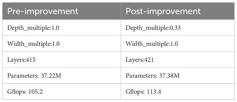
Table 1 Comparison of network model parameters.

As can be seen from the data in the table, we keep the original network width coefficient in the improved network, reduce the depth coefficient of the network to realize the scaling of the network channel, and substantially enhance the computational ability of the model under the condition of small increase in the number of network layers and parameters. Therefore, it can be demonstrated that the improved Biff module can substantially enhance the computational power of the network at the cost of a small increase in parameters. Subsequently, the effectiveness of the Biff module in target detection will be verified for enhancement.

To assess the effectiveness of the Biff module, this study conducted experiments using the Visdrone2019 aerial dataset. The Visdrone2019 dataset was meticulously curated by the AISKYEYE team from the Machine Learning and Data Mining Laboratory at Tianjin University in China. This dataset encompasses information from multiple sampling points in urban and rural areas within 14 different cities across China, spanning thousands of kilometers. The dataset’s information was captured by various models of unmanned aerial vehicle (UAV) cameras and includes ten predefined categories: pedestrian, person, car, van, bus, truck, motor, bicycle, awning-tricycle, and tricycle. These data were collected using different UAV models under diverse scenarios, weather conditions, and lighting conditions. In total, the dataset comprises 10,209 static images, with 6,471 images used for model training, 548 for validation, and 3,190 for testing. The images typically exhibit high resolutions ranging from 1080p to 4k, boasting a high level of detail. Notably, the detection targets within the images tend to be small in scale, set against complex backgrounds, and often occluded by other objects, leading to relatively low mAP scores. It is precisely due to these challenges that this dataset holds immense research value, enabling researchers to explore and enhance object detection algorithms to address a variety of complex real-world application scenarios.

As shown in Figure 1, the heat map is generated after passing the input image through four CBS modules and one ELANB module in the original YOLOv7 network. In contrast, Figure 2 presents the heat map obtained after the input image passed through four CBS modules and the Biff module designed in this study. A clear comparison reveals that after processing with the Biff module, irrelevant information, such as anti-overturning barriers on the motor vehicle lanes and dividing lines on sidewalks, has been filtered out. Additionally, it is evident that the attention on distant vehicles has significantly improved through comparison.

Figure 1

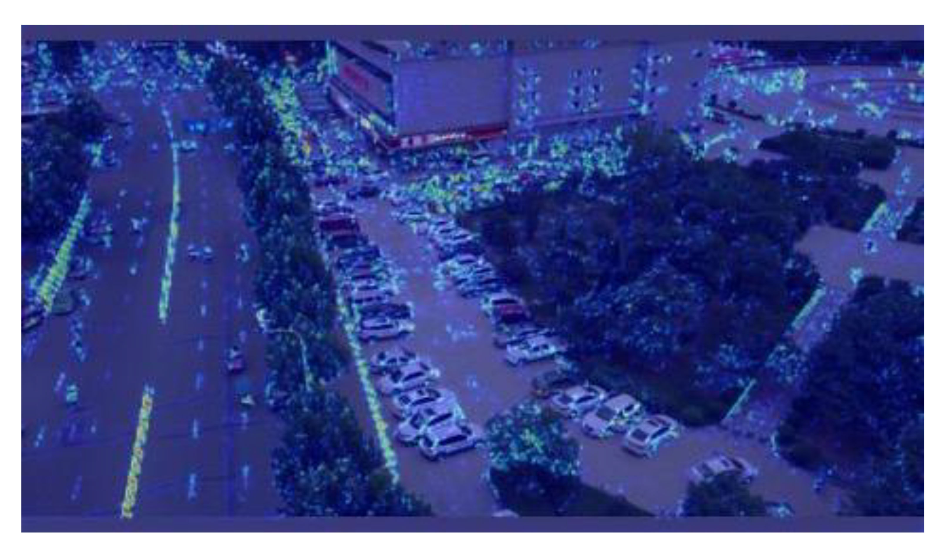
Figure 1 Heat map of YOLOv7 after four CBS modules and one ELANB module.

Figure 2

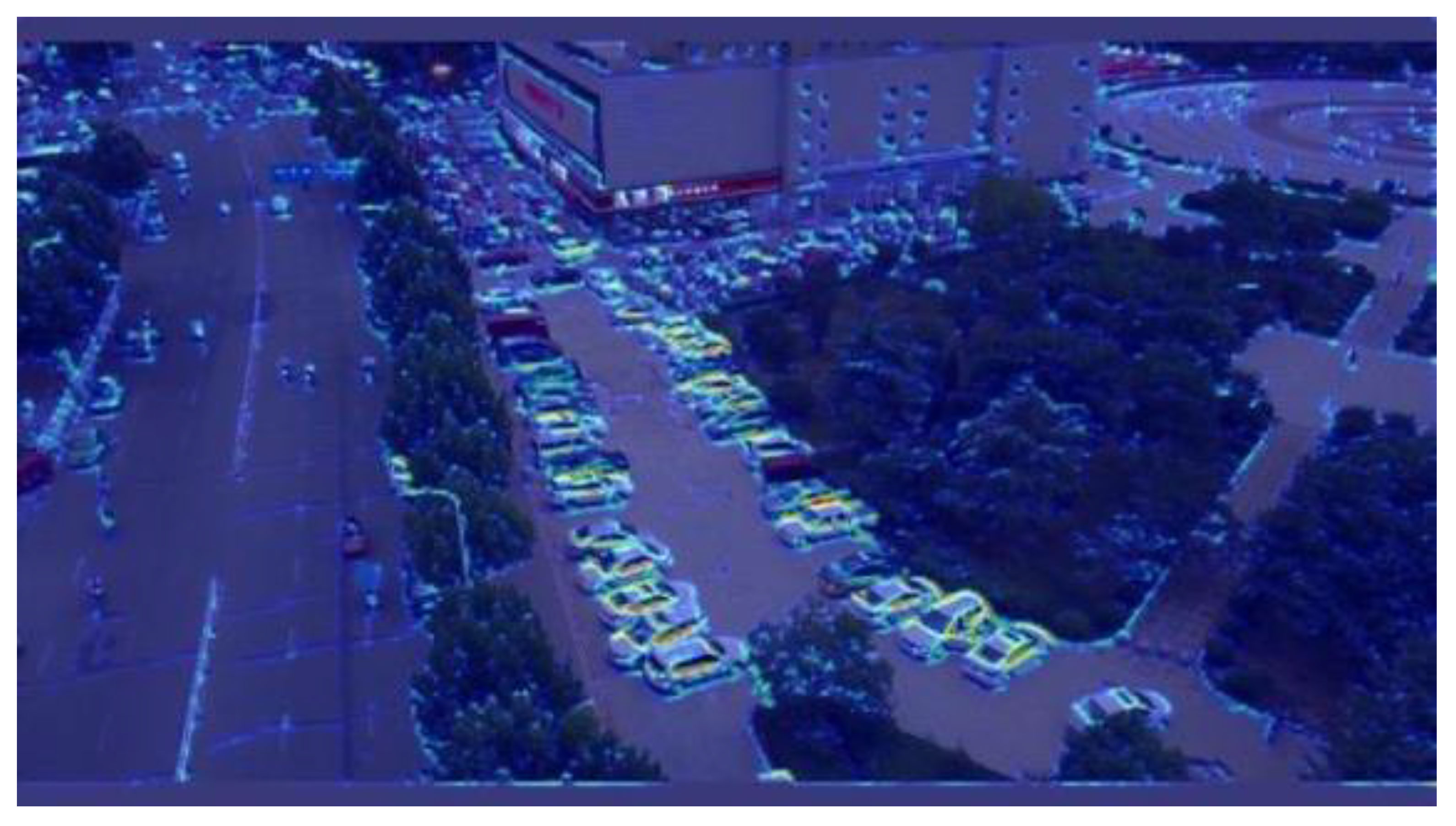
Figure 2 Heat map after 4 CBS modules and replacing ELANB module with Biff module.

3.2 Improving the YOLOv7 heat map

In urban UAV (Unmanned Aerial Vehicle) aerial images, a prevalent scenario involves a multitude of vehicle targets, often characterized by their small scale and high abundance. Accurate detection of these small targets necessitates a more precise assessment of the overlap between predicted bounding boxes and the ground truth boxes. To address this challenge, we have undertaken improvements to the original YOLOv7 algorithm by enhancing the IOU (Intersection over Union) loss function. This enhancement aims to reduce false positives and false negatives by ensuring correct matching. The original YOLOv7 algorithm utilizes the CIOU (Ni et al., 2021) (Complete Intersection over Union) loss function for IOU calculation. The CIOU is calculated as shown in Equation 23:

$\begin{array}{ll}{L}_{CIoU}=1-IoU+\frac{{\rho }^2((Bbo{x}_x,Bbo{x}_y),(PBbo{x}_x,PBo{x}_y))}{c^2}+\alpha V& (23)\end{array}$

where $\alpha$ is a balancing parameter that is not involved in the gradient calculation and is calculated as shown in Equation 24. $\rho$ is the computed Euclidean distance. $c$ is the diagonal distance of the smallest enclosure that covers both the target and the predicted bounding box. $(Bbo{x}_x,Bbo{x}_y)$ are the center coordinates of the bounding box, $(PBbo{x}_x,PBo{x}_y)$ are the center coordinates of the prediction box.

$\begin{array}{ll}\alpha =\frac{V}{(1-IoU)+V}& (24)\end{array}$

$V$ is used to calculate the consistency of the target bounding box and predicted bounding box aspect ratios, which is calculated as in Equation 25:

$\begin{array}{ll}V=\frac{4}{{\pi }^2}{(\arctan \frac{Bbo{x}_w}{Bbo{x}_h}-\arctan \frac{PBbo{x}_w}{PBbo{x}_h})}^2& (25)\end{array}$

Where $Bbo{x}_w$ and $Bbo{x}_h$ are the width and height of the bounding box respectively. $PBbo{x}_w$ and $PBbo{x}_h$ are the width and height of the prediction box respectively.

While the CIoU (Complete Intersection over Union) loss function takes into account the overlap area, center point distance, and aspect ratio in bounding box regression, it uses the relative proportion of width and height to represent aspect ratio differences, rather than employing the absolute values of width and height. Consequently, this approach can hinder the model’s effective optimization of similarity. To address this limitation, we have replaced the original CIoU loss function in YOLOv7 with the EIoU (Wu et al., 2023) (Enhanced Intersection over Union) loss function. The calculation formula for EIOU is Equation 26.

$\begin{array}{ll}\begin{array}{l}{L}_{EIoU}=1-IoU+\frac{{\rho }^2((Bbo{x}_x,Bbo{x}_y),(PBbo{x}_x,PBo{x}_y))}{c^2}\\ +\frac{{\rho }^2(Bbo{x}_w,PBbo{x}_w)}{c_{w}2}+\frac{{\rho }^2(Bbo{x}_h,PBbo{x}_h)}{c_{h}2}\end{array}& (26)\end{array}$

In this context, $c_w$ and $c_h$ refer to the width and height of the smallest bounding box that can simultaneously encompass both the target and predicted bounding boxes. The EIoU (Enhanced Intersection over Union) loss function extends the CIOU (Complete Intersection over Union) loss function by separately calculating the influence of aspect ratios on the length and width of both the target and predicted bounding boxes. This direct minimization of the disparity in width and height between the target and predicted bounding boxes aids in achieving higher localization precision in UAV aerial image detection tasks. Furthermore, it enhances convergence speed, facilitating efficient and accurate detection of small-sized vehicle targets in aerial images.

A comparison of the visualized heatmap of the original YOLOv7 version with the enhanced YOLOv7 algorithm proposed in this study is illustrated in Figures 3, 4. Our algorithm incorporates specific optimizations in the network’s backbone to better accommodate densely distributed detection targets and increase the focus on relevant objects. This contribution leads to improved predictions of detection boxes and consequently enhances the overall detection accuracy. By introducing the EIoU (Enhanced Intersection over Union) loss function to fine-tune the model training weights, we have bolstered the detection performance, particularly for small-sized targets. These heat map visualizations clearly illustrate that the enhanced algorithm, in the context of handling densely distributed small target detection tasks, has achieved significant improvements over the original YOLOv7 network.

Figure 3

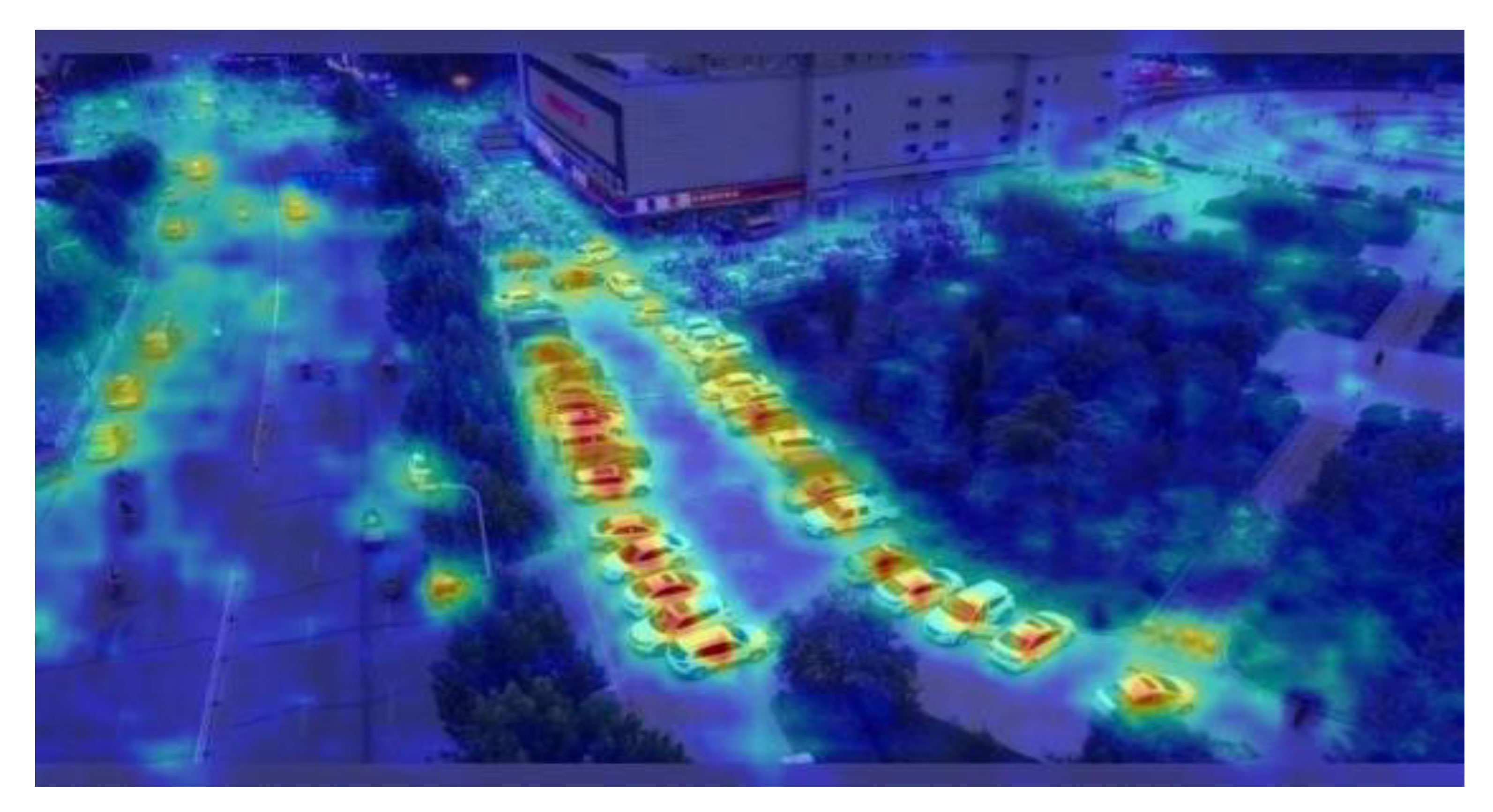
Figure 3 Original YOLOv7 heat map.

Figure 4

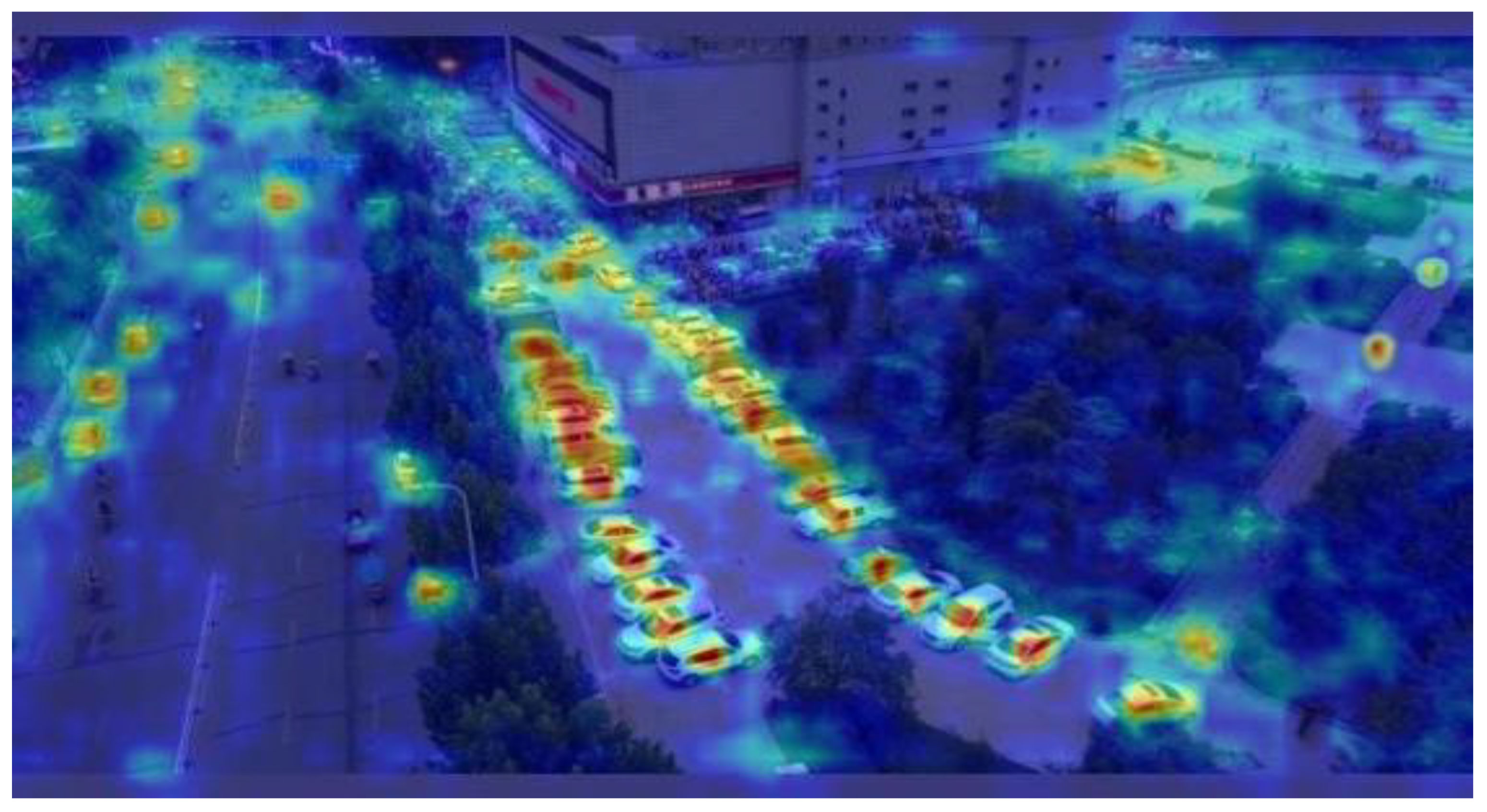
Figure 4 Improved YOLOv7 heat map.

Shown in Figure 5 is the original image from the VisDrone2019 dataset. In Figure 6 shows the performance of our enhanced YOLOv7 network in the detection task. It is clear from these figures that the algorithm proposed in this paper has the ability to accurately detect distant vehicle targets.

Figure 5

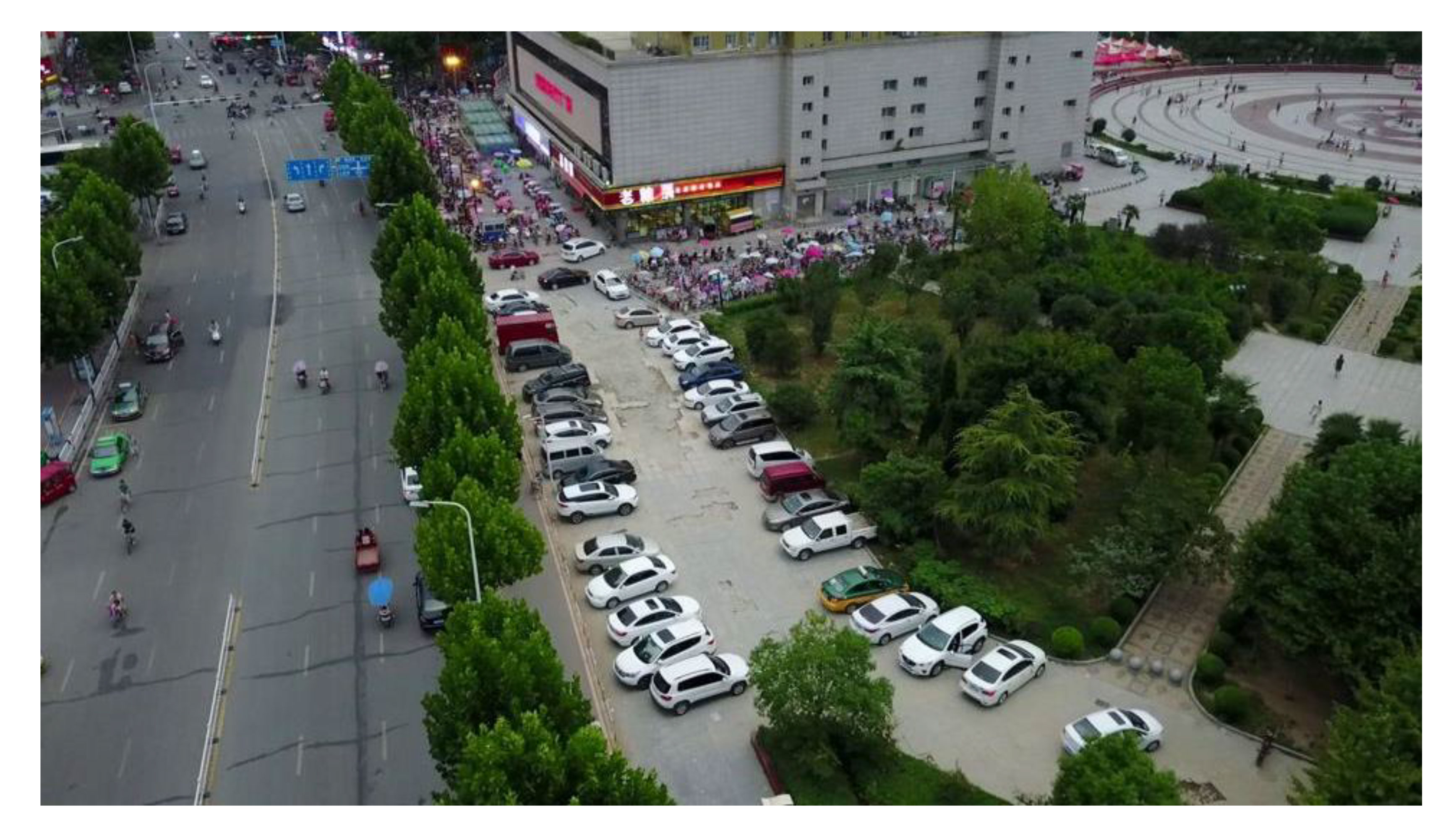
Figure 5 Original image.

Figure 6

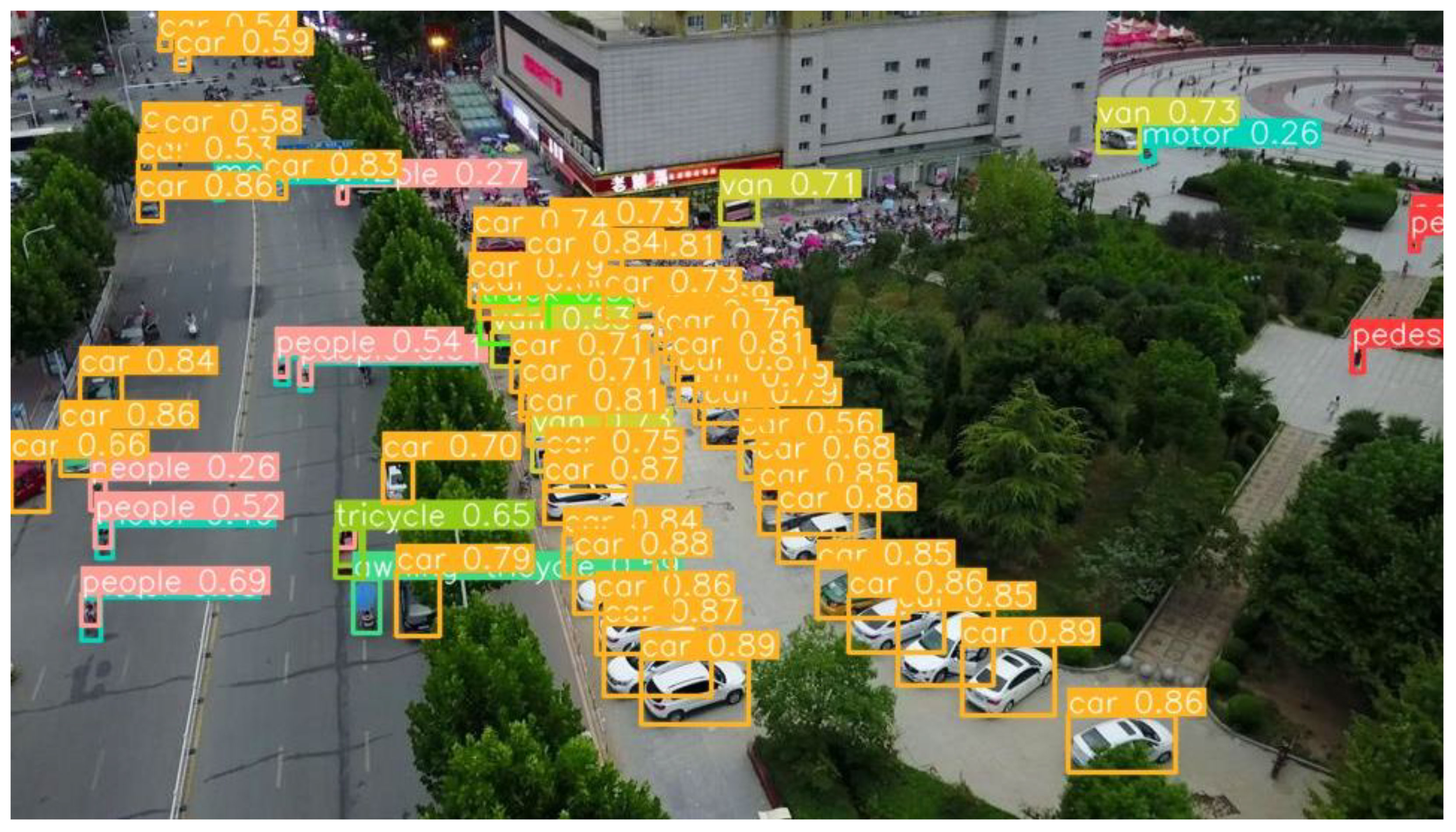
Figure 6 Improved YOLOv7 detection effect diagram.

The improved YOLOv7 network structure of this paper is shown in Figure 7, and both the Biff module and the original Biformer module are also shown in the figure. In our design, the custom-developed Biff module is indicated in red, highlighting its position within the network. The Biff module’s structural diagram is represented in blue, while the Biformer module within the Biff module is distinguished by its purple color.

Figure 7

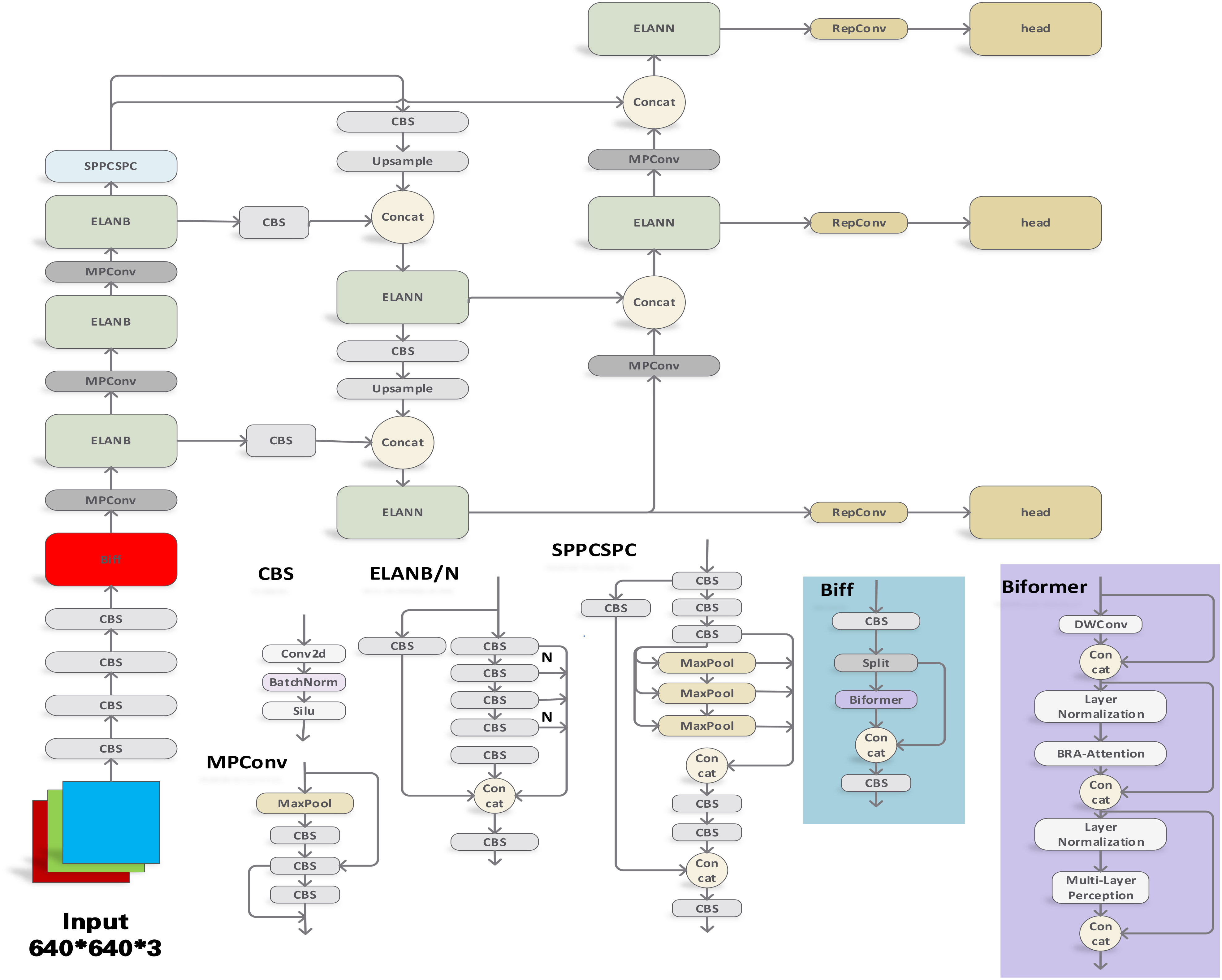
Figure 7 Improved YOLOv7 network structure diagram.

4 Evaluation of the city environmental quality

4.1 Detected vehicles and persons

We selected 600 images from the Visdrone2019 dataset for our subsequent environmental assessment research. These 600 images are categorized into four categories:

Category 1. High vegetation coverage, low human and vehicle density;

Category 2. High vegetation coverage, high human and vehicle density;

Category 3. Low vegetation coverage, low human and vehicle density;

Category 4. Low vegetation coverage, high human and vehicle density.

Each category consists of 150 images and we have selected some of the detection results to be presented in Figure 8.

Figure 8

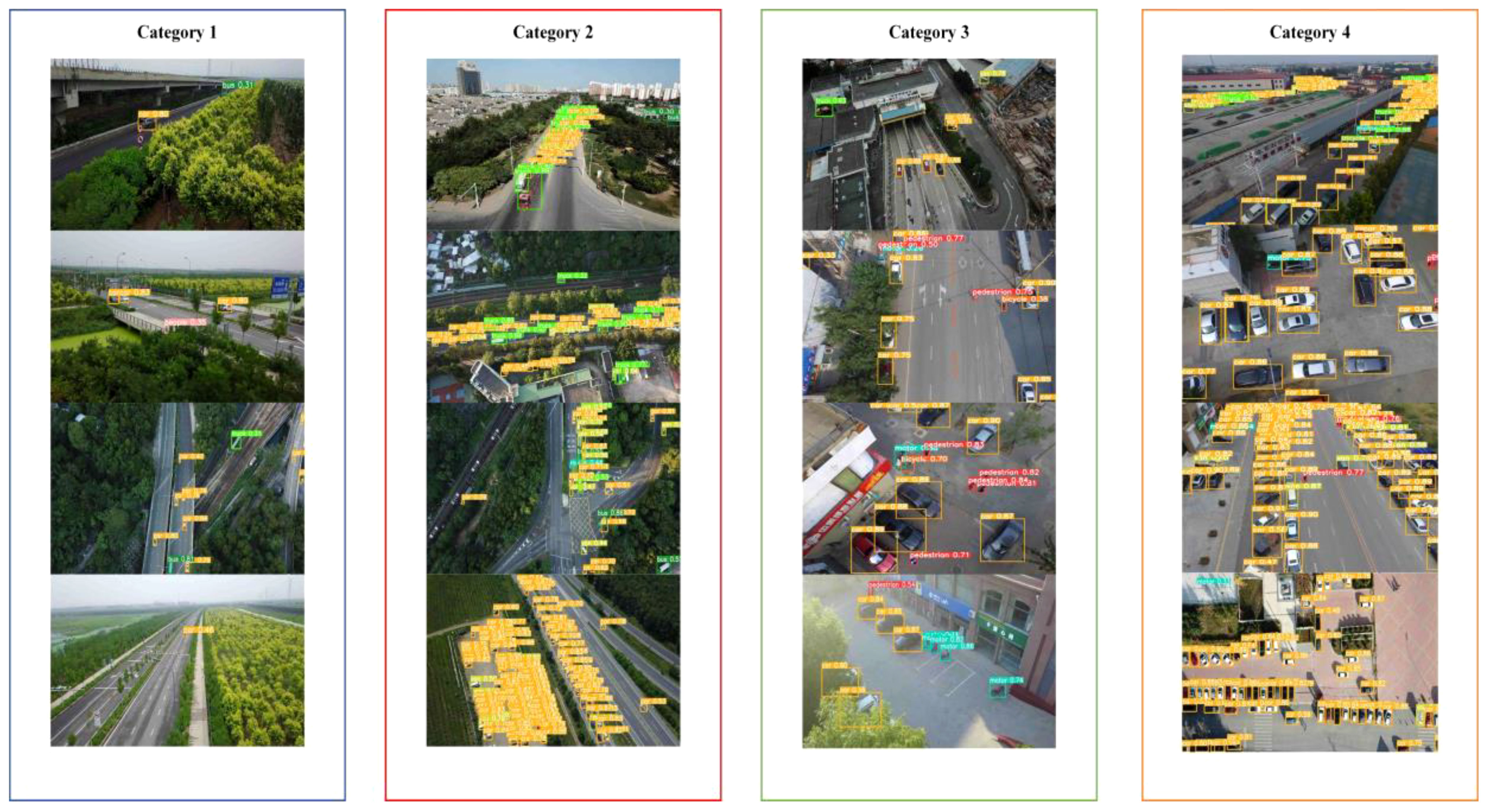
Figure 8 Effectiveness demonstration of the four categories.

The detection results shown within the blue box depict the target detection performance under conditions of high vegetation coverage and low human and vehicle density. The detection results in the red box exemplify the target detection performance under conditions of high vegetation coverage and high human and vehicle density. The green box illustrates the detection results in conditions of low vegetation coverage and low human and vehicle density, while the yellow box demonstrates the detection results in conditions of low vegetation coverage and high human and vehicle density. In the presented results, it is evident that vehicles of different scales, such as cars, buses, and motorcycles, are accurately detected.

4.2 Calculated vegetation coverage

In Figure 9 the preprocessing results of color superpixel segmentation achieved by K-means clustering algorithm are shown. In Scenes 1–2, precise segmentation of vegetation within the images has been successfully accomplished, distinguishing between buildings and barren land within green areas and isolating them from the images. In Scene 3, accurate identification of vegetation occluded by buildings is also achieved. In Scene 6, not only is extensive vegetation accurately identified, but also the fine linear green spaces between urban roads are precisely segmented. In Scenes 5–8, we observe clear segmentation results of vast and continuous vegetation areas. The green vegetation regions in the images have been accurately delineated, providing a robust foundation for subsequent vegetation coverage statistics.

Figure 9

Figure 9 Segmentation effect in different scenes.

After successfully segmenting the targeted vegetation objects within the images, their areas are computed, followed by the calculation of their proportion within the images to assess vegetation coverage. VC1 to VC8 in the figure represent different levels of vegetation coverage. When evaluating vegetation coverage, the following criteria are employed:

(1) If the percentage of vegetation objects in the image area exceeds 30%, it is categorized as high coverage, indicating a high level of urban greening.

(2) If the percentage of vegetation objects in the image area falls between 10% and 20%, it is categorized as moderate coverage, indicating a moderate level of urban greening.

If the percentage of vegetation objects in the image area is below 10%, it is categorized as low coverage, indicating a relatively low level of urban greening.

(3) This assessment method helps us gain a comprehensive understanding of urban greening and provides quantitative information regarding vegetation coverage, which is of significant importance for ecological and evolutionary research.

4.3 Number of sensitive objects

The Figure 10 demonstrates the process of utilizing the ‘detect.py’ file within the YOLOv7 model to load pre-trained model weights and perform inference on test images. The results of this inference are visually presented on the images, including detected bounding boxes, categories, and confidence scores. Additionally, in the development environment, real-time printing of the detection count for each category is provided. Through the calculation of the number of targets belonging to the ‘person’ and ‘motor vehicle’ categories, an assessment of vehicle density is conducted. This methodology aids in a deeper understanding of the distribution of vehicles within the urban environment. From Figure 10, it is apparent that we have conducted population counts for both vehicles and pedestrians in Regions 1–6 and Region 8. In Region 7, motorcycles have also been included in the count. In Region 9, we have specifically tallied motor vehicles and a modest number of pedestrians, with non-motorized vehicle categories such as bicycles excluded from the calculation. In Regions 10–16, it is evident that the population counts for different vehicle categories maintain a high level of precision. This precision plays a pivotal role in establishing a robust foundation for our subsequent ecological and environmental assessments.

Figure 10

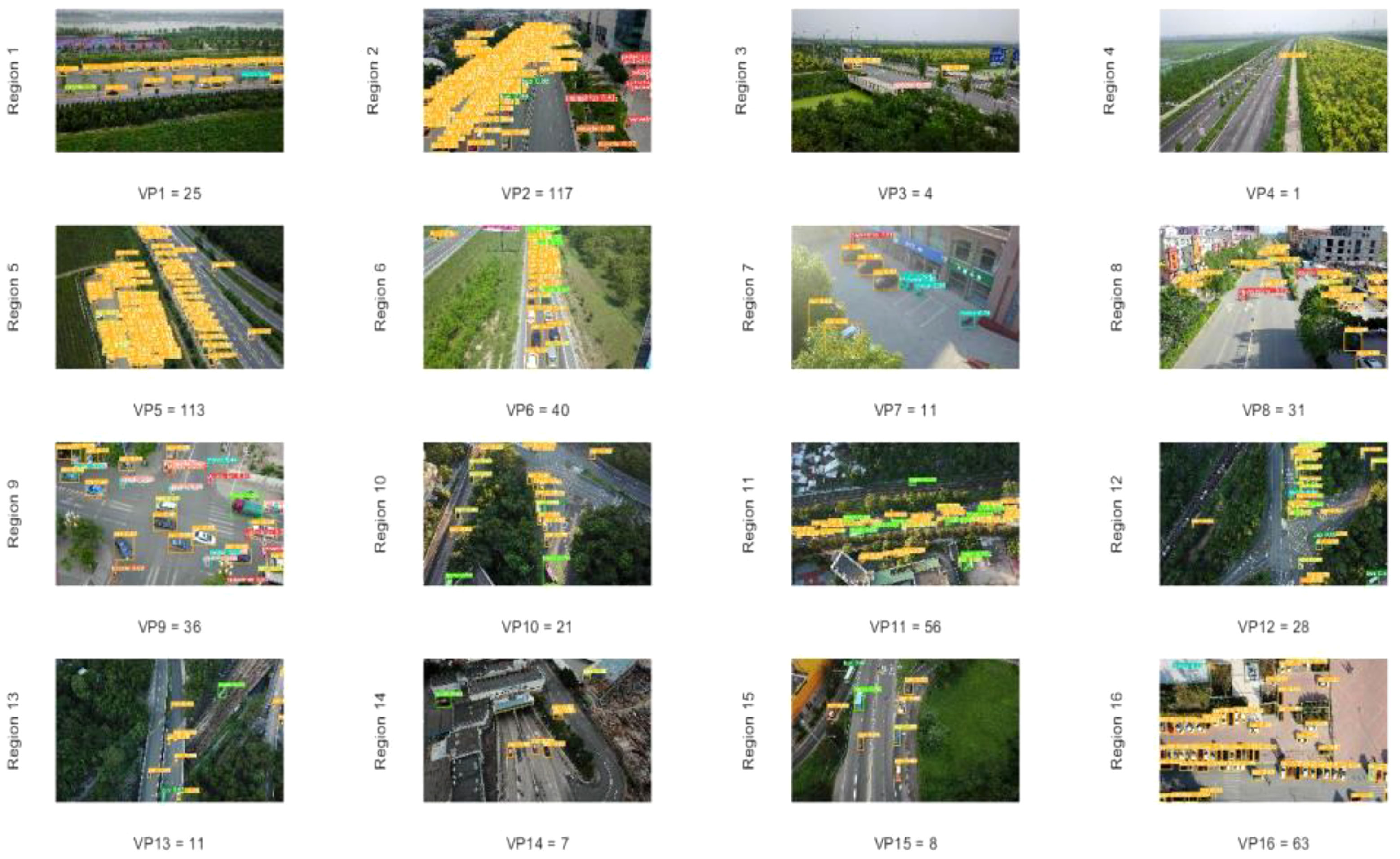
Figure 10 Statistics on the number of people and vehicles in different scenarios.

In Figure 10, we present the results of the improved YOLOv7 algorithm on test images, where it accurately detects corresponding targets based on the classification from the Visdrone2019 dataset. Subsequently, we focus on the categories of motor vehicles and humans, calculating their cumulative counts, which are prominently displayed at the bottom of the image. VP1 to VP16 respectively represent the cumulative counts for motor vehicles and humans in images 1 to 16.

4.4 Calculating the Air Quality Index

The air quality in urban areas is one of the key factors in assessing the ecological environment of cities. In order to comprehensively evaluate the urban ecological environment, data on air quality is collected from various monitoring points to assess the changes in urban air quality over a specific period. The evaluation is carried out by calculating the Air Quality Index for the urban air quality. The AQI is determined based on-air quality standards and the impact of pollutants such as particulate matter (PM₁₀, PM_2.5), sulfur dioxide (SO₂), nitrogen dioxide (NO₂), ozone (O₃), and carbon monoxide (CO) on human health, ecology, and the environment. The conventional concentrations of monitored pollutants are simplified into a single conceptual index, representing the degree of air pollution and the graded condition of air quality. The calculation method for the Air Quality Index varies by region, and different countries may adjust and modify the calculation methods based on their national circumstances. In this study, we adhere to the air quality index calculation standards of China. The AQI is calculated by Equations 27, 28:

$\begin{array}{ll}AQ=\frac{A{Q}_{high}-A{Q}_{low}}{P{C}_{high}-P{C}_{low}}(C-P{C}_{low})+A{Q}_{low}& (27)\end{array}$

where $AQ$ is the air quality sub-index and C is the pollutant concentration limit value when the actual test is conducted. $P{C}_{high}$ and $P{C}_{low}$ are obtained from Table 2 based on the values of C. $P{C}_{high}$ is the pollutant concentration limit for pollutants greater than or equal to C, and $P{C}_{low}$ is the pollutant concentration limit for pollutants less than or equal to C. $A{Q}_{high}$ is the air quality sub-index limit for $P{C}_{high}$, and $A{Q}_{low}$ is the air quality sub-index limit for $P{C}_{low}$.

Table 2

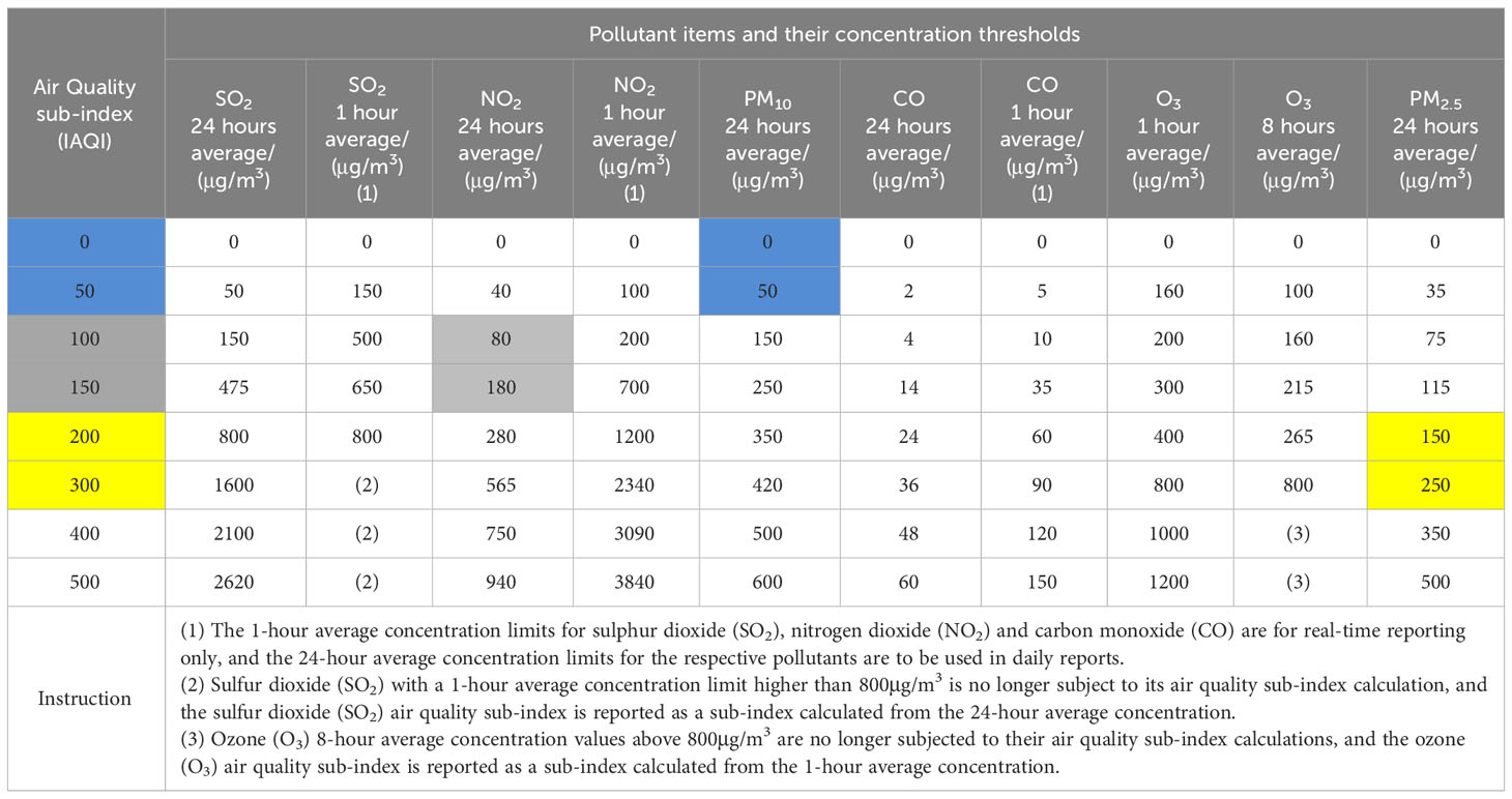
Table 2 Thresholds for pollutant concentrations corresponding to air pollution indices (Dionova et al., 2020; Popov et al., 2020), the yellow, grey and blue areas are the corresponding pollutant concentration limits and AQSIs when the 24-hour average concentration values of PM_2.5, NO₂ and PM₁₀ are 157, 150 and 40, respectively.

In Table 2, C is the current measured pollutant concentration. The limits of PM_2.5, NO₂, PM₁₀ are calculated as follows, employing 24 hours as an example. When the current measured PM_2.5 concentration value C is 157, its corresponding pollutant concentration limit and air quality sub-index limit correspond to the yellow area in the table. If the current measured concentration value C of NO₂ is 150, the corresponding pollutant concentration limits and air quality sub-index limits correspond to the gray area in the table. When the current measured PM₁₀ concentration C is 40, the corresponding pollutant concentration limits and air quality sub-index limits correspond to the blue area in the table. The limits of other pollutants can also be calculated similarly in this way.

The calculated value of AQI is usually a quantitative characterization of the pollution level of the main pollutants, which is calculated by Equation 28:

$\begin{array}{ll}AQI=\max (A{Q}_1,A{Q}_2,A{Q}_3\dots A{Q}_n)& (28)\end{array}$

According to the calculated Air Quality Index, we are able to comprehensively assess the current air quality. A lower numerical value of the Air Quality Index indicates a better current air quality, while a higher value signifies poorer air quality. This index is computed based on a comprehensive evaluation of various pollutant concentrations in the air, providing us with an effective means to objectively measure and compare air quality conditions in different regions and at different time points.

In the first two weeks of November 2023, we selected Shenyang City in Liaoning Province, China, as the monitoring site to measure the concentrations of six different pollutants in the air. In Figure 11, the distribution of concentrations for six pollutants during the first two weeks of November is presented in the form of box plots. These box plots are constructed using data information such as upper and lower bounds, median, upper and lower quartiles, and outliers. From the box plots, it is evident that concentrations of PM_2.5, PM₁₀, SO₂ and O₃ exhibited outlier values during the first two weeks of November, indicating data points that surpassed the normal range. This implies that on certain dates, pollutant concentrations exceeded the anticipated levels.

Figure 11

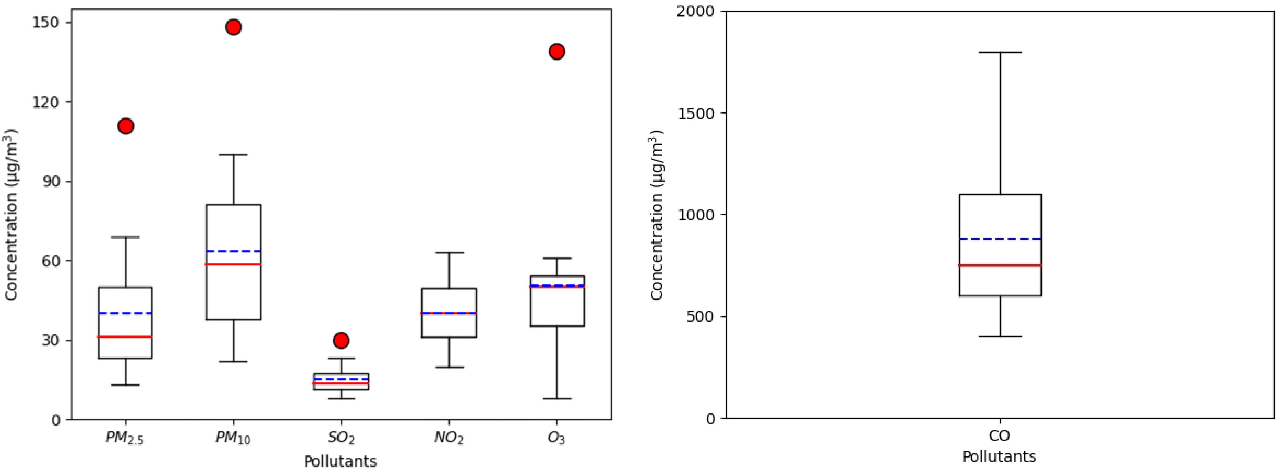
Figure 11 Box-plot of air pollutant concentration index for November 2023 in Shenyang, China. Because the concentration of CO is much higher than that of other pollutant units (left), we show a separate boxplot of CO concentration (right).

In Figure 11, the red solid line represents the median concentration of pollutants during this period, while the blue dashed line indicates the mean concentration of pollutants. Comparing the calculated median and mean values facilitates a more comprehensive analysis of the central tendencies and distribution of the overall data. The use of box plots vividly presents the dispersion of pollutant concentration data, allowing for a clear understanding of the changing trends of different pollutants during this period and identifying potential anomalies.

The assessment method of Air Quality Index is of paramount importance for maintaining the living environment of urban residents. By adopting corresponding protective measures based on different levels of air quality, the aim is to ensure the health and well-being of citizens. Utilizing the Air Quality Index to evaluate urban air quality provides an accurate depiction of the extent of atmospheric pollution. Its simplicity and clarity in calculation make it easily understandable for both urban residents and relevant authorities. This enables timely implementation of appropriate protective measures in response to diverse air quality conditions, contributing to the provision of a healthy living environment for city dwellers. Therefore, the calculation of the Air Quality Index stands as an effective tool for assessing and monitoring the ecological environment of urban areas.

4.5 Calculating the noise index

With the improvement of urban residents’ living standards and the advancement of science and technology, the number of vehicles in cities has significantly increased. Traffic noise has become one of the primary factors detrimental to the urban ecological environment. Traffic noise refers to the noise generated by various modes of transportation during their movement, primarily composed of engine noise, intake, and exhaust noise, among others. Accurate calculation and assessment of traffic noise are beneficial for evaluating the urban environment and safeguarding the health of city residents.

Currently, smartphones have become indispensable in people’s lives. Simultaneously, smartphones are equipped with rich sensors and computing capabilities that can be utilized for environmental noise monitoring (Nuryantini et al., 2021). Noise pollution in urban areas was assessed by collecting noise information using smartphone devices at selected sampling points in the Vidrone2019 aerial dataset. The chosen noise sampling locations are mainly distributed along major roads with heavy traffic flow in urban areas and near residential areas with lower vehicular density. To ensure the reliability of experimental data, noise information measurements were conducted continuously for ten minutes from different angles at each sampling point. The noise level (NL) is expressed in decibels (dB).

According to environmental noise standards, urban noise standards can be classified into five categories, with their standard values shown in Table 3.

Table 3

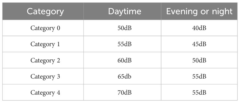
Table 3 Urban Class 5 Ambient Noise Standards.

When the noise level exceeds 65dB, the environmental noise is defined as severe noise pollution. When the noise level is within the range of 60–65dB, the environmental noise is classified as moderate noise pollution. In the case of noise levels ranging from 55–60dB, the environmental noise is designated as mild noise pollution. Class 0 and Class 1 standards are suitable for areas primarily dedicated to residential living and educational institutions. Class 2 standards are appropriate for mixed-use areas with a combination of residential, commercial, and industrial activities. Class 3 and Class 4 standards are suitable for major traffic arteries and industrial zones within urban areas. The noise levels measured from various angles in both main roads and residential areas in the city are presented in part in Figure 12.

Figure 12

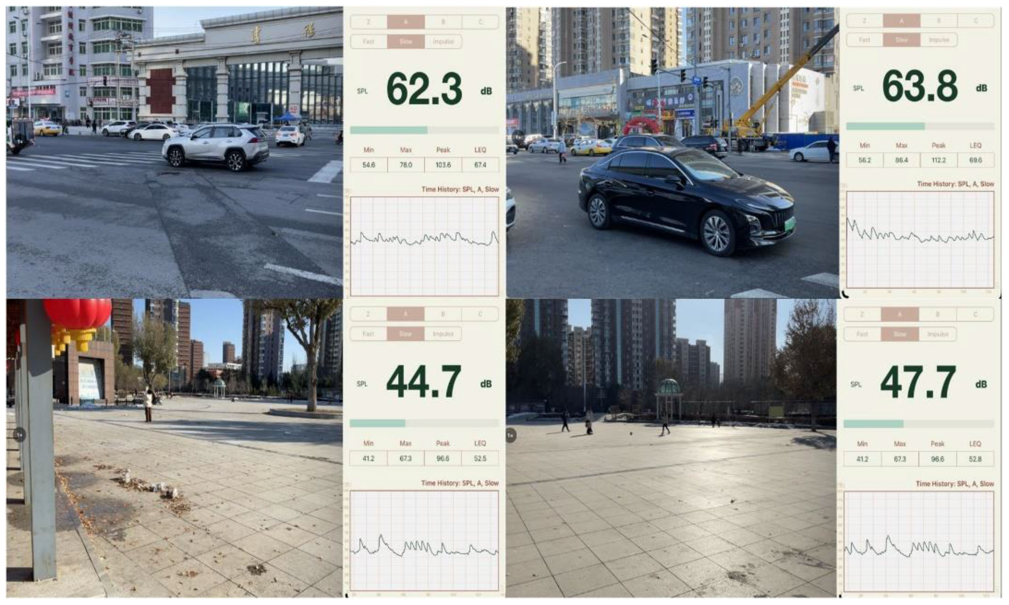
Figure 12 Measurement results of some urban trunk roads and residential areas.

In urban life, traffic noise is still primarily attributed to vehicular noise. Based on long-term measurements of noise levels, areas with significant noise pollution are identified. Strategies to mitigate noise impact in these identified areas include implementing real-time road traffic control and planting noise-reducing green belts along roadsides. These measures aim to enhance the quality of the urban ecological environment.

4.6 Score of the regional environment

Calculate the current ecological score for the urban area based on statistical data such as vegetation cover, human and vehicle density, air quality and noise levels. Calculated as shown in Equation 29:

$\begin{array}{ll}Currentenvironmentalsituation=\frac{100*VC}{\alpha *VP+\beta *AQI+\lambda *NL}& (29)\end{array}$

where VC denotes the vegetation coverage and VP denotes the cumulative sum of the counted personnel categories and vehicle categories. The paraments $\alpha$, $\beta$, $\lambda$ are the weight values corresponding to the different impact indicators in the environmental assessment, which are all non-negative and the sum of the three weight values is one.

When the computed result exceeds a certain threshold, it indicates that the self-optimization of the urban environment is insufficient, necessitating the strengthening of environmental protection measures. When the computed result falls within the range between two thresholds, the urban vegetation environment may contribute to a slight mitigation of the greenhouse effect, providing a pleasant living environment. When the computed result is below the minimum threshold, the urban vegetation environment significantly reduces the greenhouse effect, resulting in a relatively pleasant living environment. The scores calculated according to the urban condition assessment formula are shown in Figure 13, where the values of β and $\lambda$ are set to 0 and the value of α is set to 1. Only the density of people and vehicles and the vegetation cover are taken into account.

Figure 13

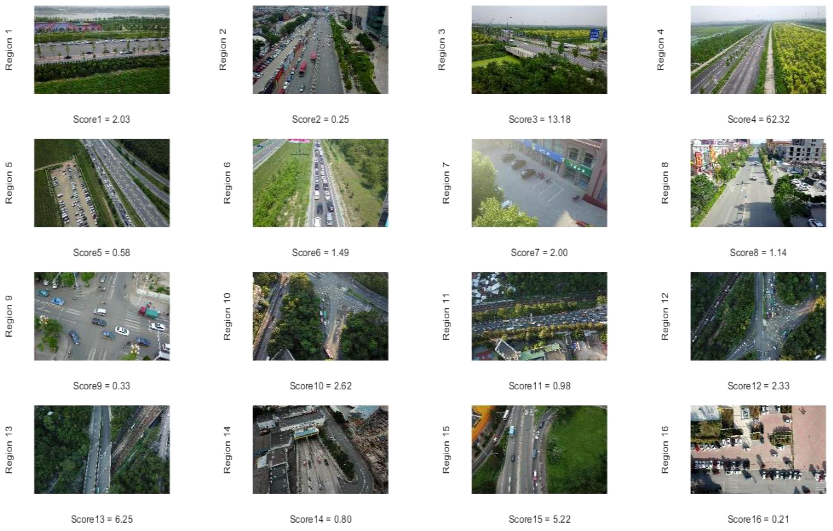
Figure 13 Environmental score assessment: $\alpha =1$, $\beta =\lambda =0$.

In Figure 13, in Regions 1–2, 5–8, 10–11, and 15, despite abundant vegetation coverage, the presence of a significant number of individuals and vehicles within the area results in a lower environmental rating. In contrast, Regions 3–4, 13, and 15 exhibit extensive vegetation coverage with fewer individuals and vehicles in the images, leading to higher environmental ratings. In Regions 9, 14, and 16, the vegetation coverage is relatively sparse, and some vehicles are still present within the area, resulting in lower environmental ratings.

In Figure 14, we utilized multiple ecological evaluation indicators to calculate the urban ecological environment scores for the current sampling points over a specific period. The ecological assessment scores according to the four different scenario categories mentioned in Section 4.1 of this paper are presented in Figure 14. As the displayed images were randomly captured at monitoring points on November 7, 2023, the AQI values for that day were employed for the air quality assessment.

Figure 14

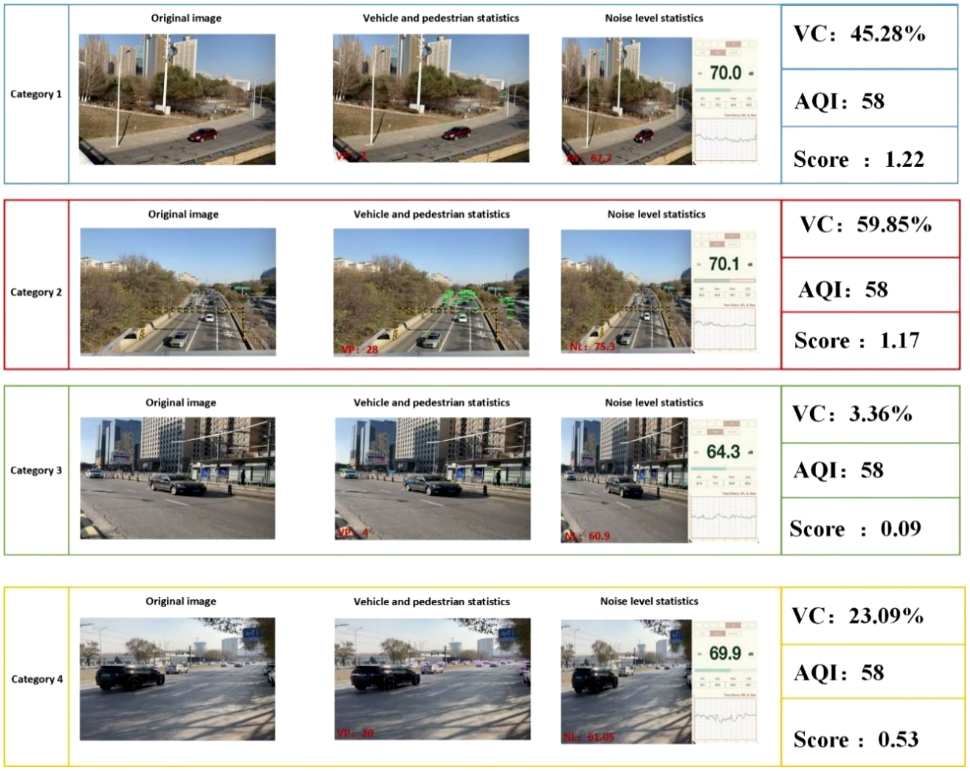
Figure 14 Environmental score assessment: $\alpha =0.4$, $\beta =\lambda =0.3$.

In this assessment, aiming for a comprehensive evaluation of urban ecological quality, we introduced information on noise levels and the Air Quality Index within the current time frame. Adjustments were made to the weight parameters in the urban environment assessment. Specifically, for this assessment, we set the value of α to 0.4, and the values of λ and β were set to 0.3 each. The use of this comprehensive assessment method aims to consider various factors affecting the urban ecological environment more comprehensively, providing more accurate results for urban ecological assessments. This approach not only takes into account factors such as vegetation coverage but also adequately considers crucial elements like noise and air quality, enhancing the effectiveness and practicality of the assessment. The careful selection of these weight parameters aims to balance the relative importance of each indicator to better reflect the overall urban ecological quality.

Observing Figure 14 it is evident that in monitoring points with higher vegetation coverage on the given day, the urban ecological environment assessment scores show a significant improvement. In the first category, due to the higher vegetation coverage in the current area, there is a relatively lower number of vehicles and pedestrians, and the air quality level on that day is considered good. Therefore, the environmental score for the first category is relatively high. In the second category, although the vegetation coverage exceeds that of the first category, the presence of a large number of moving vehicles in the current area leads to elevated noise levels. Additionally, the emission of exhaust fumes from vehicles surpasses that of the first category. Consequently, the second category, characterized by more vegetation coverage and a higher presence of vehicles and pedestrians, receives a lower score than the first category, which has more vegetation coverage and fewer vehicles and pedestrians. In the third and fourth categories, it is evident that the current area’s vegetation coverage is significantly lower than that of the first and second categories. While the noise level test may not visually depict the noise caused by construction sites around the current area, the statistical data on noise levels indicate an increasing trend in the indices. Therefore, the third category, representing cities with less vegetation and fewer vehicles and pedestrians, as well as the fourth category, denoting cities with less vegetation and more vehicles and pedestrians, exhibit urban ecological scores significantly lower than the first two categories.

In the calculation of ecological environment scores, we determined the weight values α, λ, β based on surveys conducted in different types of regions. The research results indicate that in cities with a higher concentration of industrial zones, urban residents exhibit a heightened concern for air quality. Conversely, in residential areas situated farther away from industrial zones, residents are more attentive to both current air quality and vegetation coverage in their vicinity. Consequently, we established the weight values according to the primary concerns of urban residents regarding the ecological environment, enabling the computation of the current ecological environment assessment scores. When α=1, λ=β=0, the calculated daily data yields environmental scores for four different categories, namely 22.63, 2.14, 0.84, and 1.15. In the case of α=0.5, λ=0.3, β=0.2, the computed scores for the same four categories are 1.46, 1.29, 0.11, and 0.58, respectively. This indicates that varying weight values result in distinct environmental score outcomes, thereby facilitating a differentiated assessment of the ecological environment in different regions. The judicious setting of weight values in environmental scoring allows us to more accurately reflect the concerns of residents in different areas. Furthermore, it provides robust support for the formulation of targeted measures for ecological conservation and improvement.

4.7 Comparisons with the other YOLOs

In practical applications, multi-class object detection is common, making mAP (Mean Average Precision) highly valuable for the holistic evaluation of model performance. where mAP is calculated as shown in Equation 30:

$\begin{array}{ll}mAP={\displaystyle \int P(R)dR}& (30)\end{array}$

where precision $P$ and recall $R$ are calculated as shown in Equation 31 and Equation 32, respectively.

$\begin{array}{ll}P=\frac{TP}{TP+FP}& (31)\end{array}$

$\begin{array}{ll}R=\frac{TP}{TP+FN}& (32)\end{array}$

In the formula, TP stands for True Positives, which denotes cases where the detected object is a true positive, meaning it is a real target and is correctly detected as such. FP represents False Positives, indicating instances where the detected object is a false positive, meaning it is not a real target, but the detection falsely identifies it as one. FN represents False Negatives, signifying situations where the detected object is a false negative, meaning it is a real target but is not correctly identified by the detection algorithm. P(R) represents the non-linear equation of the PR curve. mAP stands for mean Average Precision, a comprehensive performance metric. P stands for Precision, and R stands for Recall. The individual mAP curves and corresponding values for the improved YOLOv7 algorithm for the 10 different categories in the Visdrone2019 dataset are shown in Figure 15. mAP is a comprehensive performance evaluation metric that considers precision-recall curves for different categories and computes their average. mAP offers a comprehensive assessment of multi-class object detection performance.

Figure 15

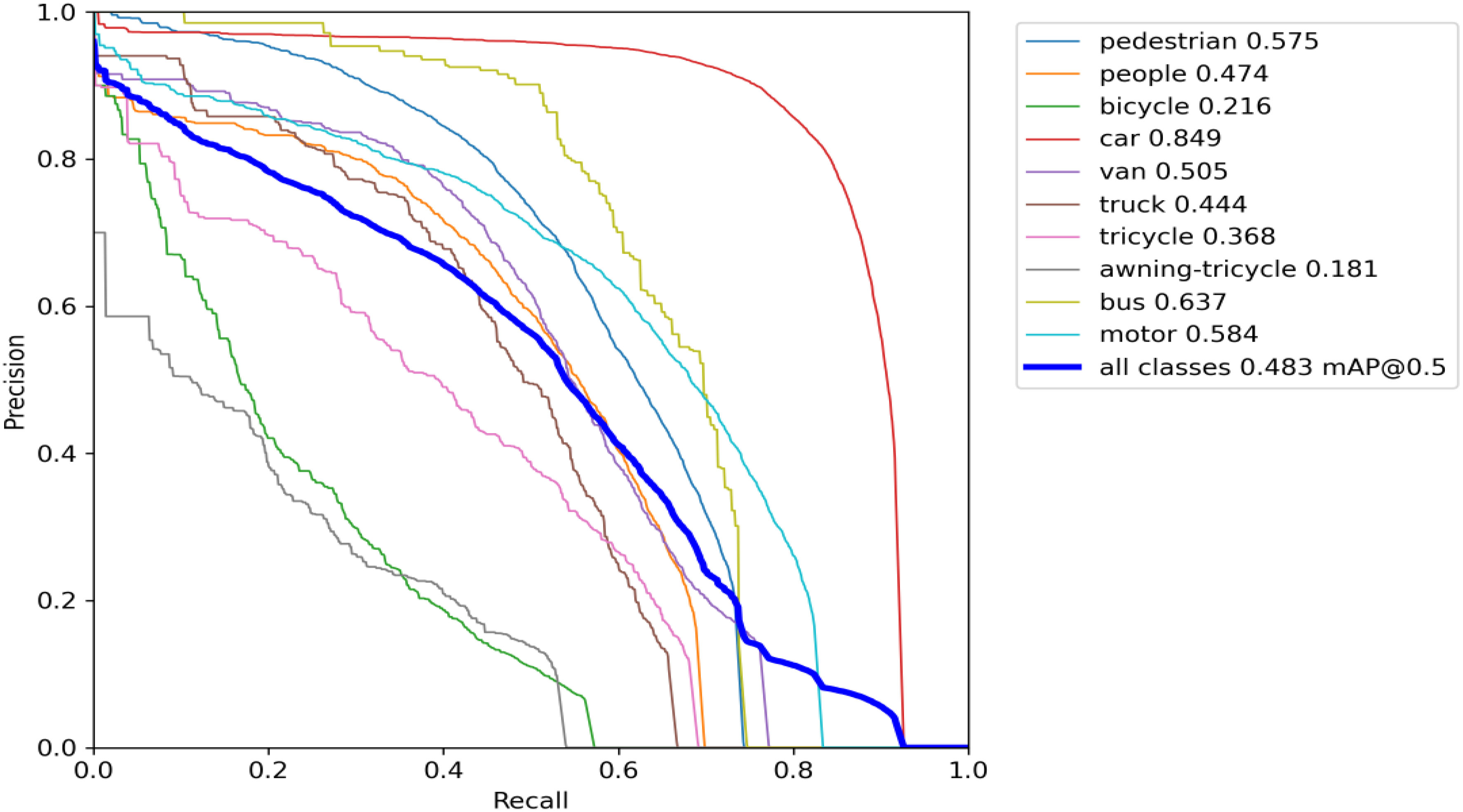
Figure 15 Map curve of the improved YOLOv7 algorithm map.

As shown in Table 4, to further validate the detection performance of our improved algorithm in this study, we conducted a comprehensive evaluation on the VisDrone2019 dataset and compared it with mainstream deep learning-based object detection algorithms. We used the mAP (Mean Average Precision) metric for comparative analysis. It can be observed that our improved algorithm achieved a relative increase of 17.6% in mAP0.5 compared to YOLOv4, an 11% improvement compared to TPH-YOLOv5, and an 8.1% enhancement compared to YOLOv8. Specifically, we noted a significant improvement in the detection accuracy of categories such as pedestrians and people within the dataset. Compared to YOLOv4, the average precision of the pedestrian category increased by 32.7%, and the average precision of the people category increased by 34.8%. For larger targets such as trucks and buses, there was also a notable improvement in detection average precision, with increases of 21.7% and 19.4%, respectively. These experimental results confirm the effective detection performance of our improved algorithm for densely populated small objects in UAV aerial imagery.

Table 4

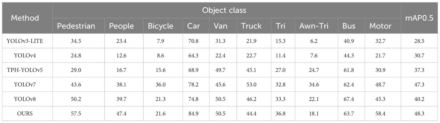
Table 4 Comparison experiments with different detection algorithms.

5 Discussion

With the rapid development of deep learning technology, the YOLOv7 algorithm, as the next-generation efficient object detection tool in the YOLO series, has found extensive applications in various ecological assessment domains. In the field of greenhouse gas assessment, the improved YOLOv7 object detection algorithm is applied for real-time detection, tracking, and counting of vehicles in urban areas. The calculated number of vehicles is then used to assess the current air quality. When there is an excess of vehicles, timely traffic flow management is implemented to reduce carbon emissions and improve urban air quality (Chung et al., 2023; Rouf et al., 2023; Zhang et al., 2023). In the domain of air pollution ecological assessment, the YOLOv7 object detection algorithm is employed to detect emission sources in low-rise suburban areas and assess the current air quality (Szczepański, 2023). In the field of vegetation ecological assessment, the YOLOv7 object detection algorithm is utilized to identify harmful plants such as weeds that may pose a threat to other vegetation. Based on the assessment results, prompt measures are taken to address areas with severe ecological damage (Gallo et al., 2023; Peng et al., 2023). Additionally, the YOLOv7 object detection algorithm is applied to extract features from trees, analyze them based on the extracted key features, and assess their health status to ensure the healthy growth of trees (Dong et al., 2023). Despite the widespread applications of the YOLOv7 algorithm in various ecological assessment domains, its application in the field of urban ecological environment assessment remains relatively limited. This presents a promising avenue for future research. By combining the YOLOv7 algorithm with urban spatial-temporal data, it becomes feasible to achieve real-time monitoring and assessment of urban ecological environments, thus promoting the preservation and sustainable development of urban ecosystems.

In the current field of ecological research, urban ecological assessment is a critically important task. Some scholars utilize fish DNA damage and physiological response biomarkers to assess the ecology of urban streams (Bae et al., 2020). Simultaneously, to gain a more comprehensive understanding of ecosystem status, other scholars employ Bayesian networks to integrate various types of knowledge, analyze the probabilities of different scenarios, and conduct risk assessments for urban ecological environments (Kaikkonen et al., 2021). Furthermore, soil cover change is a key factor in assessing ecological environments; some scholars, through spatial autocorrelation analysis, interpret risk aggregation patterns to achieve more precise ecological assessments (Ji et al., 2021). Air quality is also a crucial factor assessed by many researchers in urban ecological environments. Some researchers analyze the water-soluble concentrations of harmful heavy metals in urban roads, quantify their health risks in the urban ecology, and use this information to assess the urban ecological environment (Faisal et al., 2022). Additionally, some scholars collect dust samples along urban traffic routes, calculate the average concentrations of toxic pollutants such as lead, copper, and chromium, and use the results to evaluate the current urban air quality (Kabir et al., 2022). Some researchers construct comprehensive ecological security assessment systems for ecosystems by considering the importance of ecosystem services, ecological sensitivity, and landscape connectivity (Xu et al., 2023). Remote sensing satellite technology is commonly used to acquire ecological environment data, enabling the detection and analysis of dynamic changes in the ecological environment in urban ecological assessments. Urban ecological environments can be assessed spatially and temporally based on remote sensing surface temperature data and urban surface ecological conditions (Estoque et al., 2020; Firozjaei et al., 2020). Some scholars extract past climate change rates and extreme weather information from tree rings using new statistical tools, applying them in urban vegetation ecological assessments (Wilmking et al., 2020). Mathematical modeling and computer simulations are also employed to simulate ecosystem dynamics and responses to different pollution and management scenarios. High-resolution modeling methods and soil-crop models quantify factors such as greenhouse gas balance, allowing for the calculation of greenhouse gas emissions and the assessment of the impacts of the greenhouse effect (Launay et al., 2021). These studies have provided valuable insights for our work, emphasizing the significance of air quality and vegetation coverage as crucial factors in ecological assessment. In urban environments, vehicle exhaust emissions and the dense distribution of the population are two primary contributors to urban greenhouse gas effects. The density of people and vehicles in urban areas is a key environmental factor, second only to vegetation coverage. Consequently, we have chosen to conduct a comprehensive assessment of urban ecological environments based on combined metrics of population density, vehicle density, and vegetation coverage. This approach aims to assist governmental authorities in formulating environmental policies and facilitating more effective urban planning to enhance the quality of urban ecological environments. Past research has primarily focused on direct exploration of acquired spatiotemporal data or, based on this foundation, utilized mathematical modeling and statistical tools for analysis. During data sample collection, significant manpower and equipment are typically required. Upon completing the data collection process, mathematical models are established based on the obtained data, involving a large number of parameters that need manual design, resulting in substantial computational complexity. There has not been sufficient utilization of deep learning algorithms capable of uncovering latent features in data without the need for manual rule design. Simultaneously, there has been a lack of comprehensive analysis and research based on information detected from images. In this context, the ecological factors related to visual information have not been fully utilized. Therefore, it is a meaningful attempt for us to apply the deep learning-based YOLO target detection theory to urban ecological assessment in this paper.

The introduction of the YOLOv7 object detection algorithm offers us a novel approach to emphasize crucial visual information in ecological environment assessment. By initially conducting object detection through image data, we can recognize and highlight key elements in the environment, such as population density, vegetation coverage, and others. Subsequently, we employ the detected object information to acquire relevant data, enabling further analysis and evaluation of the ecological environment. The potential advantage of this method lies in its ability to intuitively capture visual information within the ecological environment and integrate it with traditional data, thereby providing a more comprehensive ecological assessment. To this end, we have enhanced the YOLOv7 algorithm by introducing a custom-designed Biff module in the backbone of the network model. This module serves to reduce interference from irrelevant information in the images, enhancing the focus on specific targets, and providing a solid foundation for coordinate prediction and inference stages. Furthermore, we have modified the IoU calculation section of the original network model’s loss function, replacing the original CIoU loss function with the EIoU loss function, and adjusted the training weights of the model. These adjustments have strengthened the detection performance for small-sized targets. Following 400 epochs of training and ensuring consistency between network parameters and image input sizes, we compared our improved algorithm with the original YOLOv7 and other YOLO-series-based algorithms proposed by other researchers, using the Visdrone2019 datasets. Experimental results show that, compared to the original YOLOv7, our improved algorithm achieves a one-point increase in the mAP (average precision) evaluation metric and demonstrates significant improvements in the AP values for the person, pedestrian, car, and van categories. Specifically, the AP values for the people and pedestrian categories have increased by 13.9% and 9.3%, while those for the car and van categories have improved by 6.7% and 4.9%. These results robustly affirm the effectiveness of our improved algorithm.

However, some limitations still persist in the improved algorithm. Firstly, the Visdrone2019 dataset commonly contains small-scale, densely distributed, and indistinct target instances, leading to occasional instances of missed detections. Consequently, when utilizing the improved YOLOv7 algorithm for object counting, certain biases may arise. To address this concern, we have implemented manual corrections to statistically adjust the counts of persons and vehicles. Secondly, in the context of vegetation coverage statistics, complex background scenes pose a challenge. While superpixel segmentation techniques can accurately detect and distinguish regions resembling vegetation coverage, setting uniform color thresholds for segmentation across different scenes remains problematic. Lastly, our improved YOLO object detection algorithm has yet to consider other factors affecting environmental assessment, including waste disposal, air pollution, sewage discharge, and more. In future research, we will expand the ecological and environmental image dataset to cover various situations, such as images of skies and urban rivers with different pollution levels. By applying target detection algorithms, we will identify pollution areas in the images and calculate corresponding color thresholds. Based on these color thresholds, we will compare the pollution situation in the ecological and environmental dataset to assess the current pollution level and further determine the degree of urban air and water pollution. Meanwhile, we will refine the noise data generated by factors such as pedestrian conversations, driving cars, and construction sites. By analyzing the movement status and quantity of different objects and people in the images, we will calculate the noise generated and thus evaluate the noise level at the current location. To obtain rich information using a single collection device, we plan to equip drones with sound sensors and air quality detection sensors to collect multiple urban ecological information in real-time from specific areas, thus achieving a comprehensive assessment of the current urban region’s ecological environment. Utilizing drone equipment for comprehensive urban ecological assessment will be a major direction in our future research.

6 Conclusions

The rapid development of deep learning technology has facilitated the widespread adoption of the YOLOv7 algorithm in various domains, including healthcare, industry, agriculture, and transportation, leading to a significant enhancement in the efficiency and precision of object detection. However, despite its extensive application in diverse fields, its potential utility in the realm of ecological environment assessment remains relatively unexplored. This paper presents an innovative approach that combines the improved YOLOv7 object detection algorithm with urban spatial-temporal data to enable real-time monitoring and evaluation of urban ecological environments, thereby promoting ecosystem conservation and sustainable development. This methodology holds potential significance in urban planning and environmental policy formulation, particularly in enhancing the quality of urban ecological environments. In comparison to traditional ecological assessment methods, this approach makes full use of visual information, providing fresh perspectives and directions for future research.

Nevertheless, there are still some unresolved issues associated with this objection theory for ecological environment assessment, which we intend to address in our subsequent work:

1. Addressing the issue of small-scale, densely distributed, and indistinct features in unmanned aerial vehicle (UAV) aerial datasets. This will involve making targeted improvements to the YOLOv7 network model and augmenting the existing dataset with high-quality images containing rich information to reduce biases in small object detection tasks, thereby enhancing data accuracy.

2. Tackling the complexity of background scenery in vegetation coverage statistics. The current reliance on a single threshold for precise vegetation area detection is challenging. We plan to explore updated classification algorithms, as deep learning technology continues to mature, with the expectation of achieving superior performance compared to the k-means superpixel segmentation algorithm.

3. The current paper assesses urban ecological environments solely based on the density of individuals, vehicles, and vegetation coverage, without incorporating other environmental impact factors. Our future work will involve enriching the dataset to include categories such as water quality, urban waste, and air visibility, enabling comprehensive and accurate assessments of urban environments from multiple perspectives.

Data availability statement

The datasets presented in this study can be found in online repositories. The names of the repository/repositories and accession number(s) can be found below: https://gitcode.com/mirrors/visdrone/visdrone-dataset/overview?utm_source=csdn_github_accelerator&isLogin=1.

Author contributions

TL: Writing – original draft. XH: Writing – original draft. YX: Writing – review & editing. BT: Writing – review & editing. YG: Writing – review & editing. WW: Writing – review & editing.

Funding

The author(s) declare financial support was received for the research, authorship, and/or publication of this article. This work was supported by the Liaoning Provincial Science and Technology Plan Project 2023JH2/101300205 and the Shenyang Science and Technology Plan Project 23-407-3-33. This research was funded by Shanghai High-level Base-building Project for Industrial Technology Innovation (1021GN204005-A06).

Conflict of interest

The authors declare that the research was conducted in the absence of any commercial or financial relationships that could be construed as a potential conflict of interest.

Publisher’s note

All claims expressed in this article are solely those of the authors and do not necessarily represent those of their affiliated organizations, or those of the publisher, the editors and the reviewers. Any product that may be evaluated in this article, or claim that may be made by its manufacturer, is not guaranteed or endorsed by the publisher.

References

Adibhatla V. A., Chih H. C., Hsu C. C., Cheng J., Abbod M. F., Shieh J. S. (2020). Defect detection in printed circuit boards using you-only-look-once convolutional neural networks. Electronics 9 (9), 1547. doi: 10.3390/electronics9091547

CrossRef Full Text | Google Scholar

Aguzzi J., Chatzievangelou D., Francescangeli M., Marini S., Bonofiglio F., Del Rio J., et al. (2020). The hierarchic treatment of marine ecological information from spatial networks of benthic platforms. Sensors 20 (6), 1751. doi: 10.3390/s20061751

PubMed Abstract | CrossRef Full Text | Google Scholar

Aljenaid S. S., Kadhem G. R., AlKhuzaei M. F., Alam J. B. (2022). Detecting and assessing the spatio-temporal land use land cover changes of Bahrain Island during 1986–2020 using remote sensing and GIS. Earth Syst. Environ. 6 (4), 787–802. doi: 10.1007/s41748-022-00315-z

CrossRef Full Text | Google Scholar

Arshad S., Hasan Kazmi J., Fatima M., Khan N. (2022). Change detection of land cover/land use dynamics in arid region of Bahawalpur District, Pakistan. Appl. Geomatics 14 (2), 387–403. doi: 10.1007/s12518-022-00441-3

CrossRef Full Text | Google Scholar

Bae D. Y., Atique U., Yoon J. H., Lim B. J., An K. G. (2020). Ecological risk assessment of urban streams using fish biomarkers of DNA damage and physiological responses. Polish J. Environ. Stud. 29 (2), 1–10. doi: 10.15244/pjoes/104660

CrossRef Full Text | Google Scholar

Baltodano A., Agramont A., Reusen I., van Griensven A. (2022). Land cover change and water quality: how remote sensing can help understand driver–impact relations in the Lake Titicaca Basin. Water 14 (7), 1021. doi: 10.3390/w14071021

CrossRef Full Text | Google Scholar

Bazi Y., Bashmal L., Rahhal M. M. A., Dayil R. A., Ajlan N. A. (2021). Vision transformers for remote sensing image classification. Remote Sens. 13 (3), 516. doi: 10.3390/rs13030516

CrossRef Full Text | Google Scholar

Choi R. Y., Coyner A. S., Kalpathy-Cramer J., Chiang M. F., Campbell J. P. (2020). Introduction to machine learning, neural networks, and deep learning. Trans. Vision Sci. Technol. 9 (2), 14–14. doi: 10.1167/tvst.9.2.14

CrossRef Full Text | Google Scholar

Chung M. A., Wang T. H., Lin C. W. (2023). Advancing ESG and SDGs goal 11: enhanced YOLOv7-based UAV detection for sustainable transportation in cities and communities. Urban Sci. 7 (4), 108. doi: 10.3390/urbansci7040108

CrossRef Full Text | Google Scholar

Clarke B., Otto F., Stuart-Smith R., Harrington L. (2022). Extreme weather impacts of climate change: an attribution perspective. Environ. Res.: Climate 1 (1), 012001. doi: 10.1088/2752-5295/ac6e7d

CrossRef Full Text | Google Scholar

da Silva V. S., Salami G., da Silva M. I. O., Silva E. A., Monteiro Junior J. J., Alba E. (2020). Methodological evaluation of vegetation indexes in land use and land cover (LULC) classification. Geol. Ecol. Landscapes 4 (2), 159–169. doi: 10.1080/24749508.2019.1608409

CrossRef Full Text | Google Scholar

Deng J., Lu Y., Lee V. C. S. (2021). Imaging-based crack detection on concrete surfaces using You Only Look Once network. Struct. Health Monit. 20 (2), 484–499. doi: 10.1177/1475921720938486

CrossRef Full Text | Google Scholar

Dionova B. W., Mohammed M. N., Al-Zubaidi S., Yusuf E. (2020). Environment indoor air quality assessment using fuzzy inference system. Ict Express 6 (3), 185–194. doi: 10.1016/j.icte.2020.05.007

CrossRef Full Text | Google Scholar

Dong C., Cai C., Chen S., Xu H., Yang L., Ji J., et al. (2023). Crown width extraction of metasequoia glyptostroboides using improved YOLOv7 based on UAV images. Drones 7 (6), 336. doi: 10.3390/drones7060336

CrossRef Full Text | Google Scholar

Ejigu M. T. (2021). Overview of water quality modeling. Cogent Eng. 8 (1), 1891711. doi: 10.1080/23311916.2021.1891711

CrossRef Full Text | Google Scholar

Estoque R. C., Ooba M., Seposo X. T., Togawa T., Hijioka Y., Takahashi K., et al. (2020). Heat health risk assessment in Philippine cities using remotely sensed data and social-ecological indicators. Nat. Commun. 11 (1), 1581. doi: 10.1038/s41467-020-15218-8

PubMed Abstract | CrossRef Full Text | Google Scholar

Faisal M., Wu Z., Wang H., Hussain Z., Zhou Y., Wang H. (2022). Ecological and health risk assessment of dissolved heavy metals in the urban road dust. Environ. Pollutants Bioavailability 34 (1), 102–111. doi: 10.1080/26395940.2022.2052356

CrossRef Full Text | Google Scholar

Feng D., Fu M., Sun Y., Bao W., Zhang M., Zhang Y., et al. (2021). How large-scale anthropogenic activities influence vegetation cover change in China? A Rev. Forests 12 (3), 320. doi: 10.3390/f12030320

CrossRef Full Text | Google Scholar

Firozjaei M. K., Fathololoumi S., Weng Q., Kiavarz M., Alavipanah S. K. (2020). Remotely sensed urban surface ecological index (RSUSEI): an analytical framework for assessing the surface ecological status in urban environments. Remote Sens. 12 (12), 2029. doi: 10.3390/rs12122029

CrossRef Full Text | Google Scholar

Fischer J., Riechers M., Loos J., Martin-Lopez B., Temperton V. M. (2021). Making the UN decade on ecosystem restoration a social-ecological endeavour. Trends Ecol. Evol. 36 (1), 20–28. doi: 10.1016/j.tree.2020.08.018

PubMed Abstract | CrossRef Full Text | Google Scholar

Frühe L., Cordier T., Dully V., Breiner H. W., Lentendu G., Pawlowski J., et al. (2021). Supervised machine learning is superior to indicator value inference in monitoring the environmental impacts of salmon aquaculture using eDNA metabarcodes. Mol. Ecol. 30 (13), 2988–3006. doi: 10.1111/mec.15434

PubMed Abstract | CrossRef Full Text | Google Scholar

Fu X., Wei G., Yuan X., Liang Y., Bo Y. (2023). Efficient YOLOv7-drone: an enhanced object detection approach for drone aerial imagery. Drones 7 (10), 616. doi: 10.3390/drones7100616

CrossRef Full Text | Google Scholar

Gai R., Chen N., Yuan H. (2023). A detection algorithm for cherry fruits based on the improved YOLO-v4 model. Neural Computing Appl. 35 (19), 13895–13906. doi: 10.1007/s00521-021-06029-z

CrossRef Full Text | Google Scholar

Gallo I., Rehman A. U., Dehkordi R. H., Landro N., La Grassa R., Boschetti M. (2023). Deep object detection of crop weeds: Performance of YOLOv7 on a real case dataset from UAV images. Remote Sens. 15 (2), 539. doi: 10.3390/rs15020539

CrossRef Full Text | Google Scholar

Gu S., Guenther A., Faiola C. (2021). Effects of anthropogenic and biogenic volatile organic compounds on Los Angeles air quality. Environ. Sci. Technol. 55 (18), 12191–12201. doi: 10.1021/acs.est.1c01481

PubMed Abstract | CrossRef Full Text | Google Scholar

Guanqiu W. (2021). Study on the urban agglomerations structure of the Guangdong-Hong Kong-Macao Greater Bay Area based on spatial-temporal big data. Natl. Remote Sens. Bull. 25 (2), 665–676. doi: 10.11834/jrs.20210590

CrossRef Full Text | Google Scholar

Han K. T., Ruan L. W. (2020). Effects of indoor plants on air quality: A systematic review. Environ. Sci. pollut. Res. 27 (14), 16019–16051. doi: 10.1007/s11356-020-08174-9

CrossRef Full Text | Google Scholar

Hussein K., Alkaabi K., Ghebreyesus D., Liaqat M. U., Sharif H. O. (2020). Land use/land cover change along the Eastern Coast of the UAE and its impact on flooding risk. Geomatics Natural Hazards Risk 11 (1), 112–130. doi: 10.1080/19475705.2019.1707718

CrossRef Full Text | Google Scholar

Isaifan R. J. (2020). The dramatic impact of the Coronavirus outbreak on air quality: Has it saved as much as it has killed so far? Global J. Environ. Sci. Manage. 6 (3), 275–288. doi: 10.22034/gjesm.2020.03.01

CrossRef Full Text | Google Scholar

Ji Y., Bai Z., Hui J. (2021). Landscape ecological risk assessment based on LUCC—A case study of Chaoyang county, China. Forests 12 (9), 1157. doi: 10.3390/f12091157

CrossRef Full Text | Google Scholar

Kabir M. H., Kormoker T., Shammi R. S., Tusher T. R., Islam M. S., Khan R., et al. (2022). A comprehensive assessment of heavy metal contamination in road dusts along a hectic national highway of Bangladesh: Spatial distribution, sources of contamination, ecological and human health risks. Toxin Rev. 41 (3), 860–879. doi: 10.1080/15569543.2021.1952436

CrossRef Full Text | Google Scholar

Kaikkonen L., Parviainen T., Rahikainen M., Uusitalo L., Lehikoinen A. (2021). Bayesian networks in environmental risk assessment: A review. Integrated Environ. Assess. Manage. 17 (1), 62–78. doi: 10.1002/ieam.4332

CrossRef Full Text | Google Scholar

Karn M., Sharma M. (2021). Climate change, natural calamities and the triple burden of disease. Nat. Climate Change 11 (10), 796–797. doi: 10.1038/s41558-021-01164-w

CrossRef Full Text | Google Scholar

Kiani M., Hernandez-Ramirez G., Quideau S. A. (2020). Spatial variation of soil quality indicators as a function of land use and topography. Can. J. Soil Sci. 100 (4), 463–478. doi: 10.1139/cjss-2019-0163

CrossRef Full Text | Google Scholar

Kumar A., Bhattacharya T., Mukherjee S., Sarkar B. (2022). A perspective on biochar for repairing damages in the soil–plant system caused by climate change-driven extreme weather events. Biochar 4 (1), 22. doi: 10.1007/s42773-022-00148-z

CrossRef Full Text | Google Scholar

Kusuma T. A. A. H., Usman K., Saidah S. (2021). People counting for public transportations using you only look once method. J. Teknik Informatika (Jutif) 2 (1), 57–66. doi: 10.20884/1.jutif.2021.2.2.77

CrossRef Full Text | Google Scholar

Launay C., Constantin J., Chlebowski F., Houot S., Graux A. I., Klumpp K., et al. (2021). Estimating the carbon storage potential and greenhouse gas emissions of French arable cropland using high-resolution modeling. Global Change Biol. 27 (8), 1645–1661. doi: 10.1111/gcb.15512

CrossRef Full Text | Google Scholar

Lee B. X. Y., Hadibarata T., Yuniarto A. (2020). Phytoremediation mechanisms in air pollution control: a review. Water Air Soil pollut. 231 (8), 437. doi: 10.1007/s11270-020-04813-6

CrossRef Full Text | Google Scholar

Li R., Yuan Y., Li C., Sun W., Yang M., Wang X. (2020). Environmental health and ecological risk assessment of soil heavy metal pollution in the coastal cities of Estuarine Bay—A case study of Hangzhou Bay, China. Toxics 8 (3), 75. doi: 10.3390/toxics8030075

PubMed Abstract | CrossRef Full Text | Google Scholar

Liu K., Sun Q., Sun D., Peng L., Yang M., Wang N. (2023). Underwater target detection based on improved YOLOv7. J. Mar. Sci. Eng. 11 (3), 677. doi: 10.3390/jmse11030677

CrossRef Full Text | Google Scholar

Lucas L. V., Deleersnijder E. (2020). Timescale methods for simplifying, understanding and modeling biophysical and water quality processes in coastal aquatic ecosystems: A review. Water 12 (10), 2717. doi: 10.3390/w12102717

CrossRef Full Text | Google Scholar

Majumder M., Wilmot C. (2023). Automated vehicle counting from pre-recorded video using you only look once (YOLO) object detection model. J. Imaging 9 (7), 131. doi: 10.3390/jimaging9070131

PubMed Abstract | CrossRef Full Text | Google Scholar

Meyer H., Pebesma E. (2022). Machine learning-based global maps of ecological variables and the challenge of assessing them. Nat. Commun. 13 (1), 2208. doi: 10.1038/s41467-022-29838-9

PubMed Abstract | CrossRef Full Text | Google Scholar

Mirmozaffari M., Yazdani M., Boskabadi A., Ahady Dolatsara H., Kabirifar K., Amiri Golilarz N. (2020). A novel machine learning approach combined with optimization models for eco-efficiency evaluation. Appl. Sci. 10 (15), 5210. doi: 10.3390/app10155210

CrossRef Full Text | Google Scholar

Mirzaei M., Gorji Anari M., Razavy-Toosi E., Asadi H., Moghiseh E., Saronjic N., et al. (2021). Preliminary effects of crop residue management on soil quality and crop production under different soil management regimes in corn-wheat rotation systems. Agronomy 11 (2), 302. doi: 10.3390/agronomy11020302

CrossRef Full Text | Google Scholar

Nath A., Koley B., Choudhury T., Saraswati S., Ray B. C., Um J. S., et al. (2023). Assessing coastal land-use and land-cover change dynamics using geospatial techniques. Sustainability 15 (9), 7398. doi: 10.3390/su15097398

CrossRef Full Text | Google Scholar

Ni X., Ma Z., Liu J., Shi B., Liu H. (2021). Attention network for rail surface defect detection via consistency of intersection-over-union (IoU)-guided center-point estimation. IEEE Trans. Ind. Inf. 18 (3), 1694–1705. doi: 10.1109/TII.2021.3085848

CrossRef Full Text | Google Scholar

Nuryantini A. Y., Zakwandi R., Ariayuda M. A. (2021). Home-made simple experiment to measure sound intensity using smartphones. J. Ilmiah Pendidikan Fisika Al-Biruni 10 (1), 159–166. doi: 10.24042/jipfalbiruni.v10i1.8180

CrossRef Full Text | Google Scholar

Oláh J., Aburumman N., Popp J., Khan M. A., Haddad H., Kitukutha N. (2020). Impact of Industry 4.0 on environmental sustainability. Sustainability 12 (11), 4674. doi: 10.3390/su12114674

CrossRef Full Text | Google Scholar

Onyango D. O., Ikporukpo C. O., Taiwo J. O., Opiyo S. B. (2021). Monitoring the extent and impacts of watershed urban development in the Lake Victoria Basin, Kenya, using a combination of population dynamics, remote sensing and GIS techniques. Environ. Socio-economic Stud. 9 (2), 11–25. doi: 10.2478/environ-2021-0007

CrossRef Full Text | Google Scholar

Parico A. I. B., Ahamed T. (2020). An aerial weed detection system for green onion crops using the you only look once (YOLOv3) deep learning algorithm. Eng. Agricult. Environ. Food 13 (2), 42–48. doi: 10.37221/eaef.13.2_42

CrossRef Full Text | Google Scholar

Peng M., Zhang W., Li F., Xue Q., Yuan J., An P. (2023). Weed detection with improved yolov 7. EAI Endorsed Trans. Internet Things 9 (3), e1–e1. doi: 10.4108/eetiot.v9i3.3468

CrossRef Full Text | Google Scholar

Popov O., Iatsyshyn A., Kovach V., Artemchuk V., Kameneva I., Taraduda D., et al. (2020). Risk assessment for the population of Kyiv, Ukraine as a result of atmospheric air pollution. J. Health pollut. 10 (25), 200303. doi: 10.5696/2156-9614-10.25.200303

PubMed Abstract | CrossRef Full Text | Google Scholar

Rasti B., Hong D., Hang R., Ghamisi P., Kang X., Chanussot J., et al. (2020). Feature extraction for hyperspectral imagery: The evolution from shallow to deep: Overview and toolbox. IEEE Geosci. Remote Sens. Magazine 8 (4), 60–88. doi: 10.1109/MGRS.2020.2979764

CrossRef Full Text | Google Scholar

Rouf M. A., Wu Q., Yu X., Iwahori Y., Wu H., Wang A. (2023). Real-time vehicle detection, tracking and counting system based on YOLOv7. Embedded Selforganising Syst. 10 (7), 4–8. doi: 10.14464/ess.v10i7.598

CrossRef Full Text | Google Scholar

Rousset G., Despinoy M., Schindler K., Mangeas M. (2021). Assessment of deep learning techniques for land use land cover classification in southern new Caledonia. Remote Sens. 13 (12), 2257. doi: 10.3390/rs13122257

CrossRef Full Text | Google Scholar

Sarker I. H. (2021). Deep learning: a comprehensive overview on techniques, taxonomy, applications and research directions. SN Comput. Sci. 2 (6), 420. doi: 10.1007/s42979-021-00815-1

PubMed Abstract | CrossRef Full Text | Google Scholar

Sarkodie S. A., Owusu P. A. (2021). Global assessment of environment, health and economic impact of the novel coronavirus (COVID-19). Environment Dev. Sustainability 23 (4), 5005–5015. doi: 10.1007/s10668-020-00801-2

CrossRef Full Text | Google Scholar

Schipper E. L. F. (2020). Maladaptation: when adaptation to climate change goes very wrong. One Earth 3 (4), 409–414. doi: 10.1016/j.oneear.2020.09.014

CrossRef Full Text | Google Scholar

Shao Z., Ding L., Li D., Altan O., Huq M. E., Li C. (2020). Exploring the relationship between urbanization and ecological environment using remote sensing images and statistical data: A case study in the Yangtze River Delta, China. Sustainability 12 (14), 5620. doi: 10.3390/su12145620

CrossRef Full Text | Google Scholar

Shi X., Brasseur G. P. (2020). The response in air quality to the reduction of Chinese economic activities during the COVID-19 outbreak. Geophysical Res. Lett. 47 (11), e2020GL088070. doi: 10.1029/2020GL088070

CrossRef Full Text | Google Scholar

Shi P., Li P., Li Z., Sun J., Wang D., Min Z. (2022). Effects of grass vegetation coverage and position on runoff and sediment yields on the slope of Loess Plateau, China. Agric. Water Manage. 259, 107231. doi: 10.1016/j.agwat.2021.107231

CrossRef Full Text | Google Scholar

Sippel S., Meinshausen N., Fischer E. M., Székely E., Knutti R. (2020). Climate change now detectable from any single day of weather at global scale. Nat. Climate Change 10 (1), 35–41. doi: 10.1038/s41558-019-0666-7

CrossRef Full Text | Google Scholar

Srivastava A., Chinnasamy P. (2021). Investigating impact of land-use and land cover changes on hydro-ecological balance using GIS: insights from IIT Bombay, India. SN Appl. Sci. 3 (3), 343. doi: 10.1007/s42452-021-04328-7

CrossRef Full Text | Google Scholar

Sumangala N., Kini S. (2022). A systematic review of machine learning applications in land use land cover change detection using remote sensing. Int. J. Appl. Eng. Manage. Lett. (IJAEML) 6 (2), 327–350. doi: 10.47992/IJAEML.2581.7000.0162

CrossRef Full Text | Google Scholar

Szczepański M. (2023). Vision-based detection of low-emission sources in suburban areas using unmanned aerial vehicles. Sensors 23 (4), 2235. doi: 10.3390/s23042235

PubMed Abstract | CrossRef Full Text | Google Scholar

Talukdar S., Singha P., Mahato S., Pal S., Liou Y. A., Rahman A. (2020). Land-use land-cover classification by machine learning classifiers for satellite observations—A review. Remote Sens. 12 (7), 1135. doi: 10.3390/rs12071135

CrossRef Full Text | Google Scholar

Tan Y., Cai R., Li J., Chen P., Wang M. (2021). Automatic detection of sewer defects based on improved you only look once algorithm. Automation Construction 131, 103912. doi: 10.1016/j.autcon.2021.103912

CrossRef Full Text | Google Scholar

Tummala S., Kim J., Kadry S. (2022). BreaST-Net: Multi-class classification of breast cancer from histopathological images using ensemble of swin transformers. Mathematics 10 (21), 4109. doi: 10.3390/math10214109

CrossRef Full Text | Google Scholar

van Zoest V., Osei F. B., Hoek G., Stein A. (2020). Spatio-temporal regression kriging for modelling urban NO2 concentrations. Int. J. Geographical Inf. Sci. 34 (5), 851–865. doi: 10.1080/13658816.2019.1667501

CrossRef Full Text | Google Scholar

Wilmking M., van der Maaten-Theunissen M., van der Maaten E., Scharnweber T., Buras A., Biermann C., et al. (2020). Global assessment of relationships between climate and tree growth. Global Change Biol. 26 (6), 3212–3220. doi: 10.1111/gcb.15057

CrossRef Full Text | Google Scholar

WMikhaylov A., Moiseev N., Aleshin K., Burkhardt T. (2020). Global climate change and greenhouse effect. Entrepreneurship Sustainability Issues 7 (4), 2897. doi: 10.9770/jesi.2020.7.4(21)

CrossRef Full Text | Google Scholar

Wu Y., Gao D., Fang Y., Xu X., Gao H., Ju Z. (2023). SDE-YOLO: A novel method for blood cell detection. Biomimetics 8 (5), 404. doi: 10.3390/biomimetics8050404

PubMed Abstract | CrossRef Full Text | Google Scholar

Wu G. L., Liu Y. F., Cui Z., Liu Y., Shi Z. H., Yin R., et al. (2020). Trade-off between vegetation type, soil erosion control and surface water in global semi-arid regions: A meta-analysis. J. Appl. Ecol. 57 (5), 875–885. doi: 10.1111/1365-2664.13597

CrossRef Full Text | Google Scholar

Xu X., Wang S., Yan G., He X. (2023). Ecological security assessment based on the “Importance–sensitivity–connectivity” Index and pattern construction: A case study of **liu ditch in the yellow river Basin, China. Land 12 (7), 1296. doi: 10.3390/land12071296

CrossRef Full Text | Google Scholar

Yang Z. (2021). Activation function: cell recognition based on YoLov5s/m. J. Comput. Commun. 9 (12), 1–16. doi: 10.4236/jcc.2021.912001

CrossRef Full Text | Google Scholar

Yousefi S., Pourghasemi H. R., Avand M., Janizadeh S., Tavangar S., Santosh M. (2021). Assessment of land degradation using machine-learning techniques: A case of declining rangelands. Land Degradation Dev. 32 (3), 1452–1466. doi: 10.1002/ldr.3794

CrossRef Full Text | Google Scholar

Yunus E. Ğ. İ. (2023). YOLO V7 and computer vision-based mask-wearing warning system for congested public areas. J. Institute Sci. Technol. 13 (1), 22–32. doi: 10.21597/jist.1243233

CrossRef Full Text | Google Scholar

Zaghari N., Fathy M., Jameii S. M., Shahverdy M. (2021). The improvement in obstacle detection in autonomous vehicles using YOLO non-maximum suppression fuzzy algorithm. J. Supercomputing 77 (11), 13421–13446. doi: 10.1007/s11227-021-03813-5

CrossRef Full Text | Google Scholar

Zeng X., Yu Y., Yang S., Lv Y., Sarker M. N. I. (2022). Urban resilience for urban sustainability: Concepts, dimensions, and perspectives. Sustainability 14 (5), 2481. doi: 10.3390/su14052481

CrossRef Full Text | Google Scholar

Zhang J., Zhong F., He K., Ji M., Li S., Li C. (2023). Recent Advancements and Perspectives in the Diagnosis of Skin Diseases Using Machine Learning and Deep Learning: A Review. Diagnostics 13 (23), 3506. doi: 10.3390/diagnostics13233506

PubMed Abstract | CrossRef Full Text | Google Scholar

Zhang Y., Sun Y., Wang Z., Jiang Y. (2023). YOLOv7-RAR for urban vehicle detection. Sensors 23 (4), 1801. doi: 10.3390/s23041801

PubMed Abstract | CrossRef Full Text | Google Scholar

Zhao Y., Zhang H., Zhang X., Chen X. (2021). Fire smoke detection based on target-awareness and depthwise convolutions. Multimedia Tools Appl. 80 (18), 27407–27421. doi: 10.1007/s11042-021-11037-1

CrossRef Full Text | Google Scholar