 Zheng Zhou
 Hai-Bin Xiong1,2,3
95% of researchers rate our articles as excellent or good
Learn more about the work of our research integrity team to safeguard the quality of each article we publish.
Find out more
ORIGINAL RESEARCH article
Front. Ecol. Evol. , 22 September 2023
Sec. Environmental Informatics and Remote Sensing
Volume 11 - 2023 | https://doi.org/10.3389/fevo.2023.1257854
This article is part of the Research Topic Spatial Modelling and Failure Analysis of Natural and Engineering Disasters through Data-Based Methods,volume III View all 18 articles
The response surface model has been widely used in slope reliability analysis owing to its efficiency. However, this method still has certain limitations, especially the curse of high dimensionality when considering the spatial variability of geotechnical parameters. The slice inverse regression dimensionality reduction method is efficient to obtaining the dimensionality-reduction variables from the original soil parameters space, before constructing the response surface. However, the dimensionality reduction process may cause accuracy deficiency due to the loss of variable information. An adaptive slope reliability analysis method is proposed to quantify and correct information loss and errors. Additionally, the slope failure probability based on the response surface in the dimensionality reduction space is modified to an unbiased one based on the finite model in the original space. In this study, two soil slopes considering spatial variability are taken as examples. The results illustrate that this method can effectively reduce the loss of accuracy in the dimensionality reduction process, while obtaining unbiased finite-element-based failure probability effectually. The method addresses the limitation whereby the accuracy of the dimensionality reduction process depends on the sample size and the number of dimensionality-reduction variables. Simultaneously, the proposed method significantly improves the computational efficiency of the sliced inverse regression method and realizes a reasonable dimensionality reduction effect, thereby improving the application of the response surface in practical slope reliability high-dimensional issues.
The reliability analysis of slope stability is a crucial issue in geotechnical engineering considering the uncertainties of geotechnical parameters (Deng et al., 2017; Xiao et al., 2018; Cao et al., 2019; Liu et al., 2019; Deng et al., 2020; Wang et al., 2020a; Wang et al., 2020b; Zhang et al., 2023a; Zhang et al., 2023b). Many reliability analysis methods have been proposed, such as the Monte Carlo simulation (MCS) (e.g., Griffiths and Fenton, 2004; Cho, 2007; Cho, 2010; Huang et al., 2010; Li et al., 2015b), first-order second moment method (FOSM) (e.g., Christian et al., 1994; Hassan and Wolff, 1999; Xue and Gavin, 2007), first-order reliability method (FORM) (e.g., Low and Tang, 1997; Low and Tang, 2004; Ji, 2014; Low, 2014; Zeng and Jimenez, 2014), second-order reliability method (SORM) (e.g., Cho, 2009; Low, 2014), and advanced Monte Carlo simulation, Subset Simulation method (e.g., Au and Beck, 2001; Wang et al., 2010; Wang et al., 2011; Li et al., 2016b). Among these, the failure probability must be obtained by repeating slope stability analysis, which is computationally expensive. In recent years, the response surface (RS) method has been proven to be an effective method to solve this issue. The principle is to develop an RS with small computational cost to approximate the original complex model; therefore, the slope reliability can be estimated almost negligible costs based on this RS model.
To date, many scholars have proposed various RS models to perform slope reliability analysis, such as the quadratic polynomial (Xu and Low, 2006; Ji and Low, 2012; Ji et al., 2012; Tan et al., 2013), Hermite polynomial chaos expansion (Jiang et al., 2014; Jiang et al., 2015; Li et al., 2016c), support vector machine (Tan et al., 2011; Li et al., 2013; Chang et al., 2020; Huang et al., 2020a), neural network (Cho, 2009; Tan et al., 2011; Piliounis and Lagaros, 2014; Huang et al., 2020c), and Kriging model (Luo et al., 2012a; Luo et al., 2012b; Zhang et al., 2013). Although the RS model has been widely used in reliability problems, several challenges remain to be resolved. The curse of high dimensionality is a major criticism restricting the application of RS in reliability analysis. When the dimensionality increases rapidly, the number of required training samples is dramatically increased to develop more complex RS forms. This computational burden may even be higher than the direct Monte Carlo methods, which is contrary to the original purpose of establishing response surfaces. In slope reliability analysis, as the inherent spatial variability of soil properties is one of the most significant geotechnical uncertainties affecting the slope failure mechanism (Christian et al., 1994; Griffiths and Fenton, 2004; Wang et al., 2011; Huang et al., 2013; Li et al., 2015a; Li et al., 2016a; Li et al., 2016b; Xiao et al., 2016; Xiao et al., 2017; Jiang et al., 2018; Li et al., 2019a; Varkey et al., 2019; Huang et al., 2020b; Deng et al., 2022; Nie et al., 2023; Zhang et al., 2023c), the curse of high dimensionality is particularly when the spatial variability of soil parameters is simulated using random fields.
Two dimensionality reduction techniques are usually used to solve high-dimensional problems: simplifying the RS form and reducing the number of random variables. In the former, different methods are applied to constructing the sparse structure of the polynomial chaos model, such as the stepwise regression technique (Blatman and Sudret, 2010) or the least-angle regression technique (Blatman and Sudret, 2011), the weighted 𝓁1 minimization algorithm with a priori information (Peng et al., 2014), and the Bayesian compressed sensing technique (Zhou et al., 2020), while other researchers constructed the sparse RS based on different basic terms, such as support vector regression (Cheng and Lu, 2018) and the quadratic polynomial (Guimarães et al., 2018). However, the computational costs of developing sparse forms remain still large when considering more time-consuming and complex models with a large number of random variables (Al-Bittar and Soubra, 2014).
The latter reduces the random variables and then develops an RS model with dimensionality-reduced parameters. Al-Bittar and Soubra (2014) applied the Sobol index of global sensitivity analysis to recognize significant input variables. However, it may lose efficiency when the contributions of each variable are similar. Rotation-based linear mapping techniques (Constantine et al., 2014; Yang et al., 2016) required partial derivatives of input variables and output, which may be computationally expensive. Alternatively, the input variables are linearly combined and transformed into a new dimensionality-reduced space, such as principal component analysis (PCA) (Jolliffe, 2002) and sliced inverse regression (SIR) (Li, 2000; Pan and Dias, 2017; Li et al., 2019b; Deng et al., 2021). Specifically, PCA takes the principle of maximizing the variance to linearly combine the original space. The effectiveness of the PCA method depends on the data structure of the input variables, which is not efficient when the input variables are independent or low correlated. The SIR method linearly transforms the original space into the dimensionality-reduced space using the relationship between response values and input variables, which makes it more efficient than the PCA method in independent soil parameters of random fields. However, subsequent studies found that the accuracy of the SIR method depends on the initial training sample size. In addition, both two dimensionality reduction techniques would lose some accuracy due to the loss of variable information in the dimensionality reduction process. There are few reasonable solutions for quantifying and correcting information loss and errors in the dimensionality reduction process.
In this study, an adaptive reliability analysis method is proposed to solve the curse of high dimensionality of the RS method and problem-dependent accuracy of the SIR method, which integrates the dimensionality reduction method, active learning method, and response conditioning method. This method can correct the information deficiency in the process of SIR dimensionality reduction and generate unbiased reliability results with low variability for slope stability in spatially varying soils. The SIR method is firstly introduced to reduce the random variables, and the accuracy-dependent problem of the SIR method is discussed, as described in Section 2. In Section 3, the adaptive reliability analysis corrects the preliminary slope reliability analysis results of the RS model in a dimensionality-reduced space to an unbiased target reliability based on the finite element (FE) model in the original space. The method uses representative samples from the response conditioning method to iteratively update the principal direction of the SIR and the RS model near the failure domain to obtain a stable unbiased target reliability. Furthermore, two slope examples considering the spatial variability are studied in Section 4 and Section 5 to validate the capacity of this method.
In slope reliability analysis, the geotechnical parameters with spatial variability are non-negligible indicators that affect the slope failure mode and its stability. When the random field is applied to simulate the spatial variability, a large number of spatially correlated random variables are generated, causing the curse of high dimensionality in slope reliability analysis. Taking the Karhunen–Loève expansion method (Li and Der Kiureghian, 1993; Phoon et al., 2002) as an example, the log-normal random field R can be described as a set of independent standard normal random variables, ξ = [ξ1, ξ2, …, ξr]T:
where μ and σ represent the mean and standard deviation of normal random field ln(R); r is the truncated number of the first largest eigenvalues and the corresponding eigenvectors, λi and φx,i (i = 1, 2,…, r), at locations x, which is determined by the required accuracy of random field discretization, such as 95% (Phoon et al., 2002; Jiang et al., 2014; Xiao et al., 2015). Although the Karhunen–Loève expansion method can reduce the number of random variables by converting the number of coordinate points at different locations into the number of expansion terms, it is affected by the type of the correlation function, the autocorrelation distance, and the scale of the random field. It may require a large number of truncation terms, r, to meet the accuracy requirement.
To reduce the large number of truncation terms, r, the SIR method is utilized in this study for further dimensionality reduction. The basic idea of the SIR method is to construct a smaller number of linear combinations from the original high-dimensional variables and to develop new variables in low-dimensional space. To ensure that each linear combination component reflects more original information, an eigenvalue decomposition of the covariance matrix V of ξ is applied, as shown in the following equation:
where βj represents the eigenvector and λj represents the eigenvalue of the covariance matrix V of dimension r.
Before the eigenvalue decomposition, the SIR method usually divides the original space according to the relationship between ξ and its response value, Y, and obtains the covariance matrix of conditional expectation E(ξ|Y), which makes it easier to determine the principal direction (see Figure 1). In the following example, N is set as the number of training samples, (ξ,Y). The SIR algorithm is shown in the following steps:
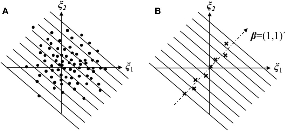
Figure 1 Schematic diagram of sliced inverse regression.
(i) Standardize the input variables of ξ and sort the training samples by the value of the response value of Y.
(ii) Divide the sorted training samples as evenly as possible into H slices, S1, S2,…, SH (see Figure 1A); the number of samples in each slice is approximated as nh = N/H. The previous studies have stated that a certain range of H has no significant influence on the dimensionality-reduced results of SIR (Li, 2000).
(iii) Calculate the mean of each slice of ξ; the conditional expectation is set as , h=1, …, H, i=1,…, nh.
(iv) Calculate the covariance matrix () of the mean of each slice, with the corresponding weight for each sample set as nh/N.
where () represents the mean value of the input variables ξ at all sample points; T denotes the matrix transpose.
(v) Calculate the eigenvalues and eigenvectors of the covariance matrix to determine the principal direction of the SIR algorithm, as shown in the following equation:
where eigenvector represents the respective vector in the jth direction of SIR (i.e., β = (1,1) as the eigenvector between ξ1 and ξ2; see Figure 1B). Normally, the first d large vectors are regarded as the principal direction (Pan and Dias, 2017).
(vi) Obtain new variables by conducting a linear combination of the original variables ξ according to the principal directions of SIR. The first d larger direction vectors correspond to d new variables, i.e.,
The ability to obtain finite and large eigenvalues of λj determines the effectiveness of SIR dimensionality reduction methods. Compared with SIR, the PCA method directly uses the covariance matrix of ξ for the eigenvalue decomposition without preprocessing. However, the PCA method has certain limitations; for instance, the same principal direction may be obtained based on two samples with the same distribution and different response values. In contrast, SIR explores the inverse regression curve of the conditional expectation E(ξ|Y) to investigate how the associated ξ changes with Y. The eigenvalue decomposition according to the covariance matrix of E(ξ|Y) can obtain the principal direction effectively. However, the accuracy of the SIR method is parameter-dependent and information loss will increase with the decrease of the initial training sample size. Taking the arithmetic examples (Rackwitz (2001); Pan and Dias, 2017) as an example to explain the information loss:
where ζi, i = 1, …, r denotes random variables with independent lognormal distributions, where the mean value is 1 and the standard deviation is 0.2; r represents the dimensionality of the random variable. To quantify the information loss and error in the SIR dimensionality reduction process, the root mean square error (ε) and the correlation coefficient (ρ) between the original space and the dimensionality-reduced space are used as indicators. The root mean square error (ε) is calculated as
where Nt denotes the test sample number, GRS is the response value in the dimensionality-reduced space calculated based on the RS, and G is the actual value in the original space calculated by Eq(5).
As shown in Figure 2, the dimensionality reduction of SIR is more effective than the PCA method in random variables. In the SIR method, the first three larger eigenvalues can be selected from 40 random variables and the value of the fourth eigenvalue quickly decays to 10−20, while in the PCA method, the values of eigenvalues of random variables are nearly the same and it is difficult to select the main eigenvalues and directions for constructing new dimension-reduced variables.
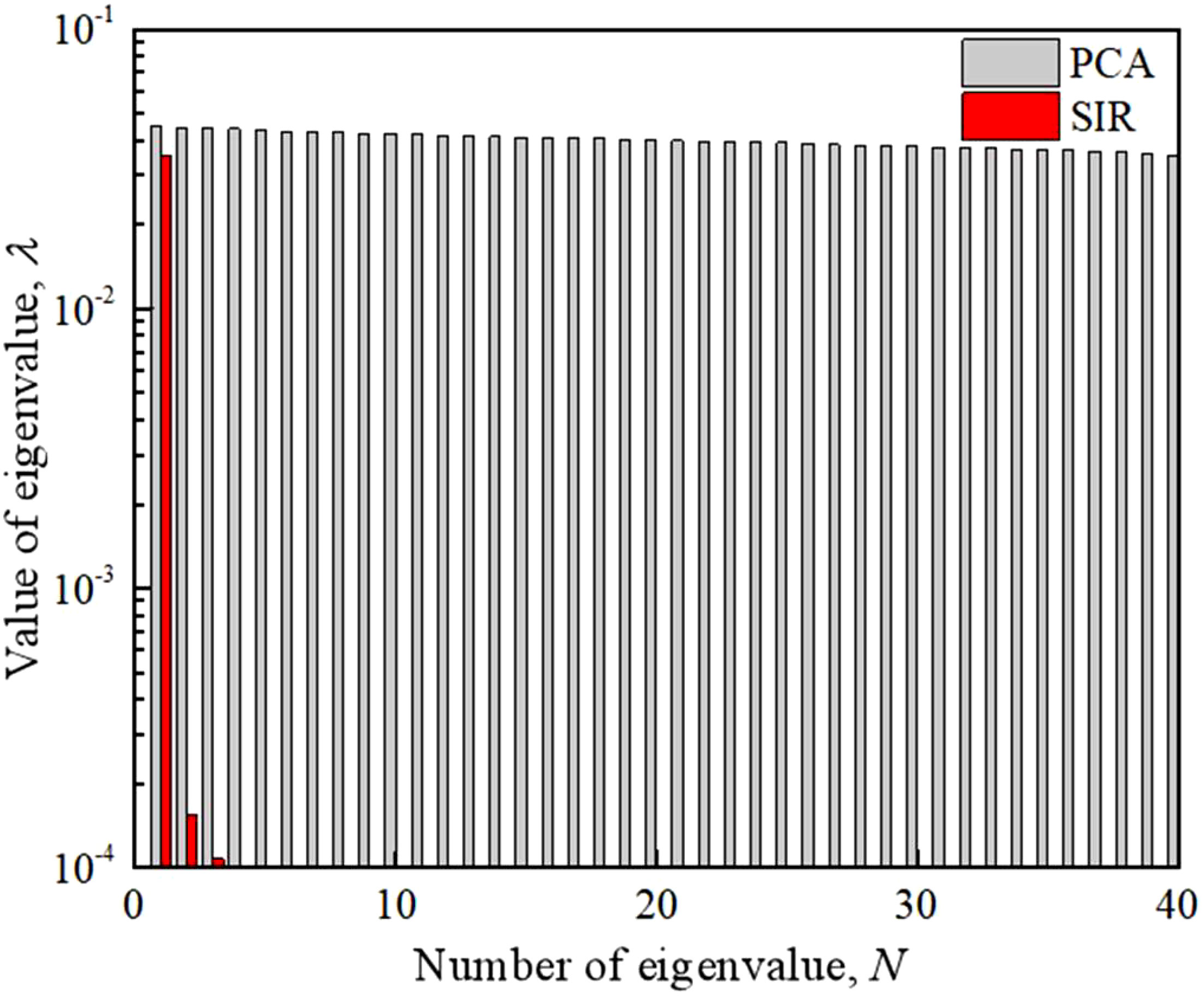
Figure 2 Comparison of dimensionality reduction effect between PCA and SIR.
Then, the accuracy of SIR with different parameters is shown in Figure 3, varying in the number of training samples, number of variables in the original (r = 20, 200, and 1,000), and number of variables in the dimensionality-reduced space (d = 3, 10, and 20). Larger training samples cause a higher accuracy in the dimensionality reduction, which can be proved by the Fisher consistency property (Li, 2000). When the number of training samples increases infinitely, the statistical value of the sample data approximates the true distribution and the principal direction in dimensionality-reduced space can unbiasedly simulate the original space. However, the huge computational cost with larger training samples is impractical, which contradicts the original intention of dimensionality reduction for higher efficiency. In addition, when the number of random variables and training samples (r = 20 N =100) are fixed, different dimensionality-reduced variables (d = 2, 4, 6) will cause different accuracy loss, with the correlation coefficient obtained as 0.912, 0.987, and 0.992, ϵ as 0.370, 0.145, and 0.112, respectively. It can be observed that the accuracy of the SIR method is a parameter-dependent method. Hence, this study proposes an adaptive slope reliability analysis method to quantify and correct errors in the dimensionality reduction process of the SIR method and obtain an unbiased reliability estimation while neglecting the initial error.
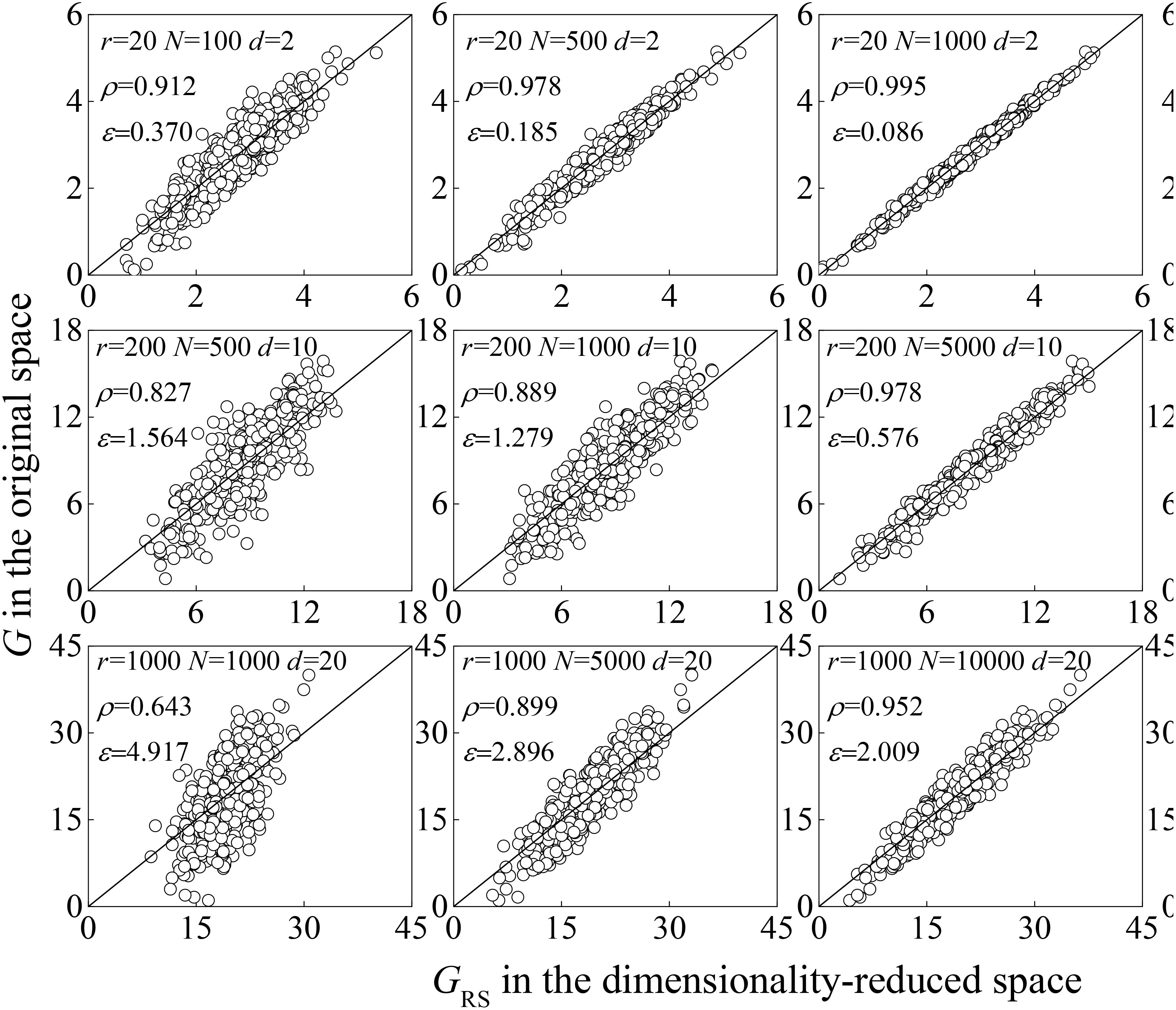
Figure 3 Information loss of SIR due to dimensionality reduction.
In this section, the adaptive reliability method is used to address the accuracy-dependent problem of the SIR method to reduce the information loss with limited training samples. The principle is to use the response conditioning method (Au, 2007) to improve the accuracy of the result efficiently based on the correlation between the simple and complex models, such that it is consistent with the unbiased complex model. In this study, the RS model in the dimensionality-reduced space is regarded as the simple model and the FE model in the original space is regarded as the complex model. In addition, compared with the traditional response conditioning method, the simple models are gradually iteratively updated, which is similar to the idea of active learning (Echard et al., 2011; Dubourg et al., 2013; Marelli and Sudret, 2018). This mitigates the requirement for a highly correlated and accurate initial dimensionality-reduced space. It consists of three steps (see Figure 4): initial SIR dimensionality reduction and preliminary reliability analysis, which determines the principal directions of SIR based on the limited training samples and then constructs the RS model in the dimensionality-reduced space; target reliability analysis, which selects sample points in the dimensionality-reduced space and transforms them into the original space to recalculated in FE model, and to obtain an unbiased estimate of the reliability with the response conditioning method; and the adaptive update strategy, which appends representative samples in original space to the training samples and updates the SIR principal direction and RS model until convergence is attained.
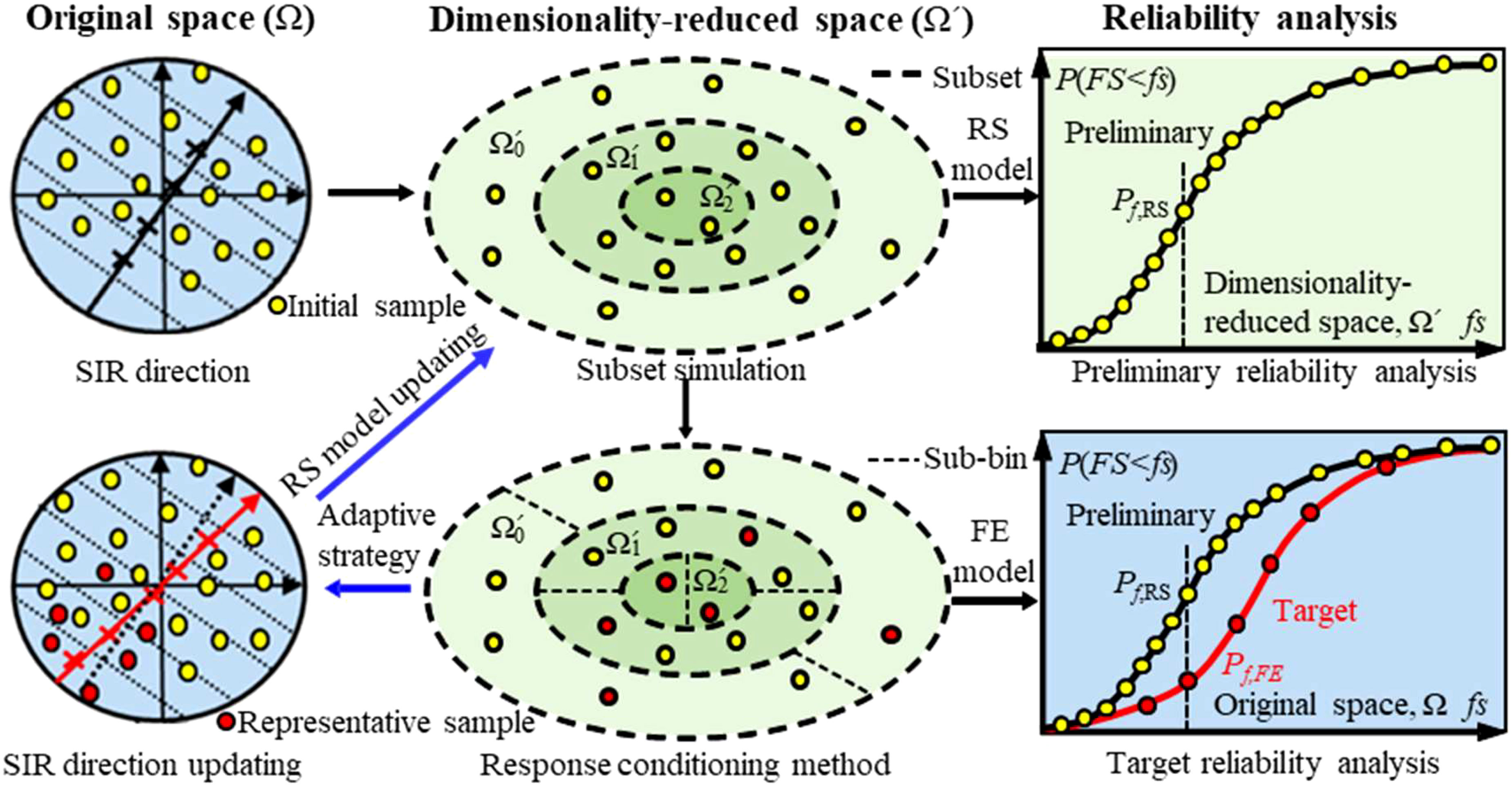
Figure 4 Schematic diagram of adaptive slope reliability analysis based on SIR.
The original and dimensionality-reduced space are defined as Ω and Ω´, respectively. The SIR principal directions are obtained from the original space samples (ξ, Y). Furthermore, the original space samples are transformed into new samples (ω, Y) in the dimensionality-reduced space Ω´. Based on the dimensionality-reduced samples, the simplest commonly used quadratic RS model without cross terms is constructed in this study. The original quadratic RS model is expressed as:
where M(ξ) is the original RS model containing 2r+1 basis terms [1, ξi, ξi2, …]; [a0, a11, …, a1r, a21, …, a2r] are the unknown coefficients; r is the input variable dimension in the original space; ξ are the variables in the original space.
The RS model in dimensionality-reduced space is rewritten as:
where M’(ω) is the RS model in dimensionality-reduced space containing 2d+1 basis terms [1, ωj, ωj2, …] and ω are the dimensionality-reduced variables, obtaining through the linear combination of ξ.
Subset simulations (Au and Beck, 2001; Li et al., 2016b) are then performed to analyze the slope reliability based on the RS model. The principle is that the occurrence of a small failure probability event can be expressed as the product of the larger conditional probabilities of a series of intermediate events. In this process, for an m-level subset simulation, the entire dimensionality-reduced space Ω´ is divided into m+1 mutually exclusive and completely exhaustive subsets of Ωk´, k = 0, 1,…, m, which are divided according to intermediate failure events {fs1, fs2, …, fsm}, as shown in Figure 4. The preliminary slope failure probability of Pf,RS is calculated using the following equation (Au and Beck, 2001; Xiao et al., 2016; Zhou et al., 2021).
where FRS = {FSRS < fs} represents the slope failure event obtained based on the RS in the dimensionality-reduced space and IRS,kj represents the failure indicator function for the jth sample in subset Ωk´ (i.e., IRS,kj = 1 if FSRS,kj < fs; otherwise, IRS,kj = 0). P(Ωk´) represents the occurrence probability of the subset Ωk´(P(Ωk´) = p0k(1−p0), k = 0, 1, …, m−1 or P(Ωk’) = p0k, k = m), where m-level subset simulation contains mNl (1 − p0) + p0Nl samples and Nl is the sample size in each simulation level. As the principal direction of the SIR method directly determines the characteristic of the dimensionality-reduced space, if the direction does not accurately reflect the characteristics of the original space, the RS in the dimensionality-reduced space will cause large accuracy loss compared with the original finite-element model. This accuracy loss caused by the inappropriate dimensionality reduction direction is extremely evident when there are insufficient training samples. Thus, target reliability analysis is applied to quantify and correct this loss.
Although the deviation of the SIR principal direction leads to a larger deviation in the RS model, the dimensionality-reduced space still has a certain correlation with the original space. Therefore, the samples in the dimensionality-reduced space can be selected using the response conditioning method (Au, 2007) and transformed into the original space to recalculate in the finite-element model, thereby correcting the preliminary slope failure probability to an unbiased estimate, as shown in Figure 4. This process is based on the sub-binning strategy (Au, 2007), where the main principle is that the samples in the adjacent region share similar properties, i.e., when an interval is sufficiently small, a random sample from that interval can be used to characterize its properties, such as whether the interval fails or not. Only the selected samples are recalculated for reevaluating the failure probability in the FE model so that a large amount of FE analyses can be avoided.
For instance, each subset Ωk´ is further divided into Ns equal sub-bins Ωkj, j = 1, 2, …, Ns. Taking advantage of the correlation between the dimensionality-reduced and original spaces, one sample from each sub-bin is randomly selected as a representative sample to revert to the original space Ω and its response value FSFE is obtained in the FE model. According to the response conditioning method, the target reliability failure probability Pf,FE is calculated as (Li et al., 2016a; Xiao et al., 2016; Zhou et al., 2021):
where FRS = {FSFE< fs} is the slope failure event obtained based on the FE model in the original space Ωk; IFE,kj is the failure indicator function for the representative sample Ωkj in the original space (i.e., IFE,kj = 1 if FSFE,kj < fs; otherwise, IFE,kj = 0). As the representative samples are drawn from the dimensionality-reduced space, the subset Ωk (i.e., P(Wk´) = P(Wk)), occurs with the same probability as the subset Ωk´ [i.e., P(Ωk´) = P(Ωk)]. The accuracy of Pf,FE depends on the correlation of the dimensionality-reduced space with the original space, which is directly determined by whether the SIR principal direction is accurate or not. If the SIR principal direction is inconsistent with the true direction, the Pf,FE will have a relatively high variability. In this case, the principal directions of the SIR and RS coefficients are updated gradually by an adaptive strategy to obtain a stable target reliability estimate.
This adaptive strategy progressively updates the simple model (the principal direction of the SIR and preliminary RS models), in order to reduce the variability of Pf,FE due to the deviation of SIR principal direction. This process utilizes the representative samples in target reliability analysis, to update the covariance matrix (Vnew), the corresponding eigenvalues (λnew), and eigenvectors (βnew). Therefore, the SIR principal direction and the RS model are updated with special emphasis nearby the failure domain (Bucher and Bourgund, 1990; Ji and Low, 2012). Subsequently, a second round including preliminary and target reliability analysis is performed. The detailed implementation procedures of the adaptive strategy are provided in Figure 5. The SIR directions and the RS model are gradually updated by active learning and a final unbiased reliability estimate with small variability is obtained, until the correlation (ρRS,FE) between RS values in the dimensionality-reduced space and FE values in the original space reaches convergence (ρRS,FE ≤ 5%). Owing to the different sample weights in each subset, the correlation between the two modes can be calculated as (Li et al., 2016a):
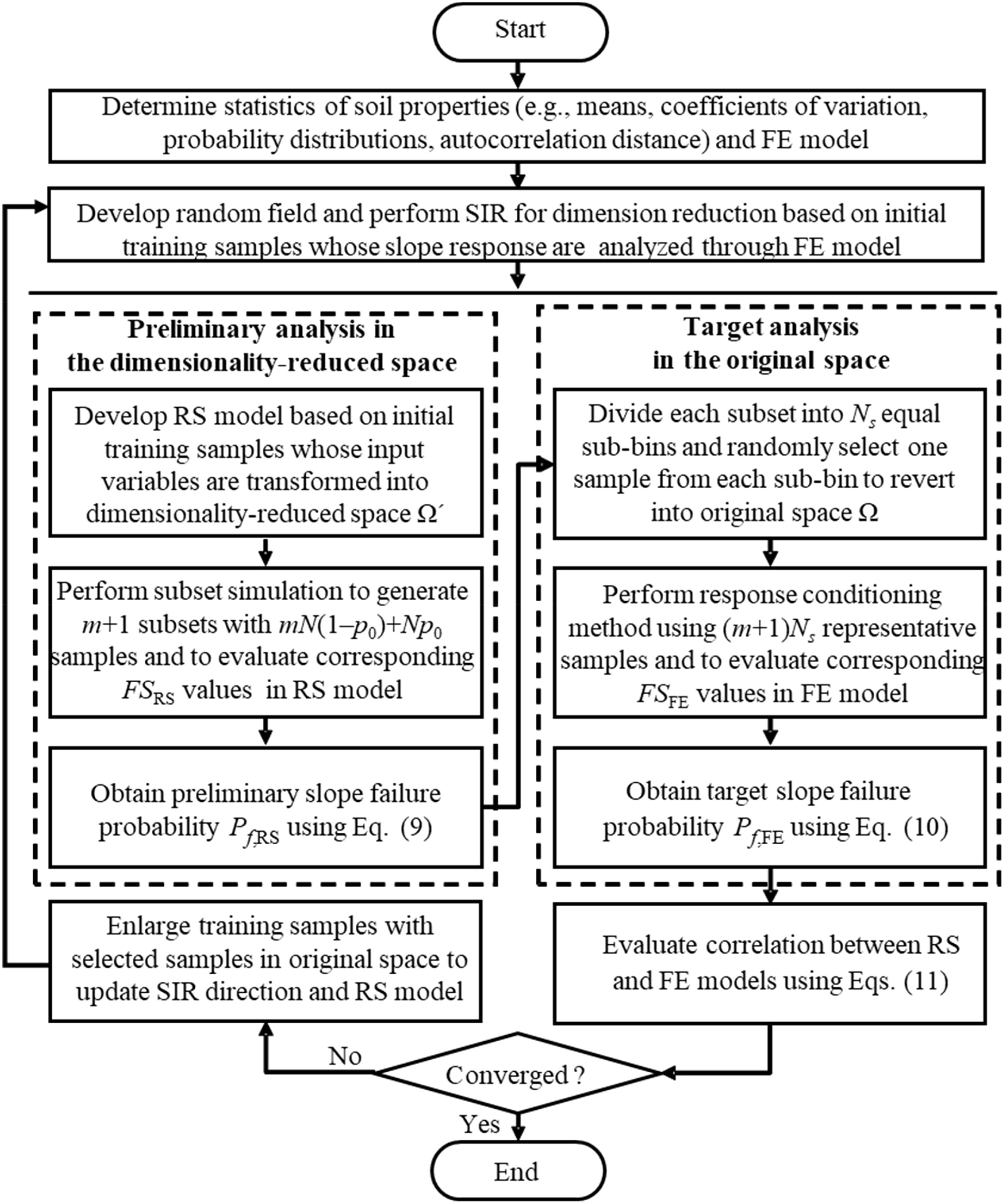
Figure 5 Implementation procedures of adaptive slope reliability analysis based on SIR.
where and represent the expectation and variance, respectively; X represents FSRS, FSFE, or FSRS × FSFE, whereas Xk represents samples of X in the subset of Ωk.
An undrained homogeneous soil slope (Griffiths and Fenton, 2004; Jiang et al., 2015) is taken as an example to illustrate the effect of the proposed method. With a height of 5 m and angle of 26.6° (see Figure 6), the slope has its undrained shear strength and unit weight as 23 kPa and 20 kN/m3, respectively (see Table 1). In this study, deterministic analysis was performed by the shear strength reduction technique in FE analysis. The soil is modeled by an elastic-perfectly plastic constitutive model with the Mohr–Coulomb failure criterion. The deterministic safety factor is 1.348 through the shear strength reduction technique in FE analysis, which is close to 1.356 using the simplified Bishop method (Cho, 2010; Jiang et al., 2015), similar to Zhou et al. (2021). The slope reliability analysis was then repeated by implementing a non-intrusive stochastic manner (Li et al., 2016b). In the slope reliability analysis considering the spatial variability of slope soil properties, two different cases are conducted: the first is the benchmark case with a coefficient of variation (COV) of 0.15 and an autocorrelation function of squared exponential (QExp); the second is the high-dimensional case with identical parameters, but with a single exponential autocorrelation function (SExp). Considering the non-negativity of the parameters, log-normal random fields are used for the undrained shear strength.
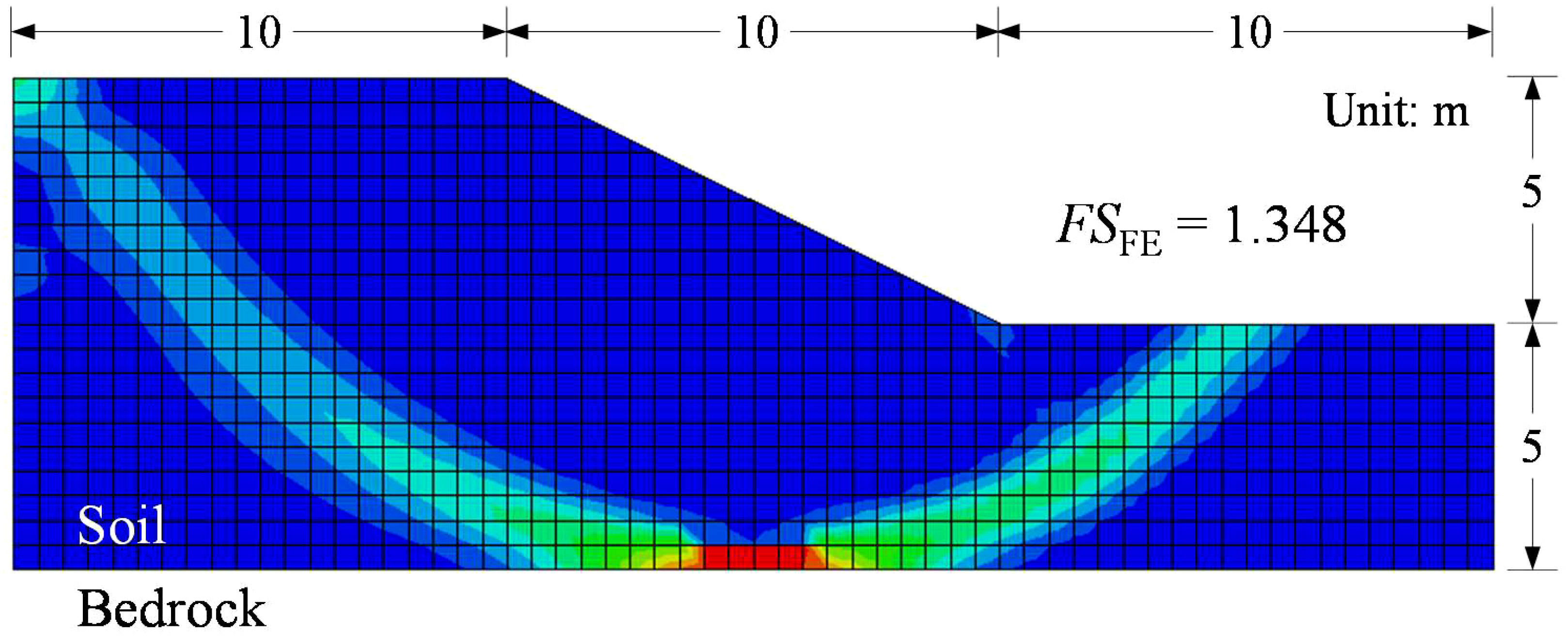
Figure 6 Deterministic FE analysis of the undrained slope example.
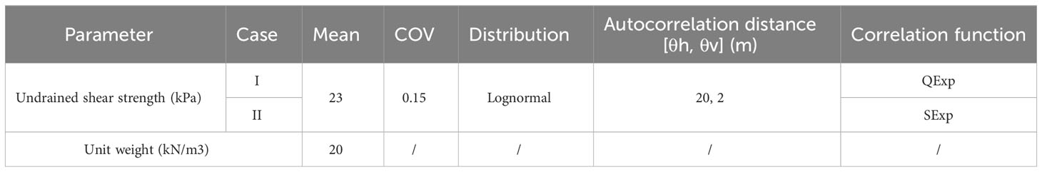
Table 1 Soil properties for the undrained slope example.
In this case, 15 random variables are required to meet the 95% accuracy of K–L random field discretization. A total of 30 training samples (ξ, Y) are required as training samples to compare the dimensionality reduction effect of SIR and PCA. As shown in Figure 7, the first two larger eigenvalues of SIR are 0.937 and 0.427 in the initial iteration, and from the third eigenvalue, its value decays from 10−16 to 10−18. Therefore, the eigenvectors corresponding to these two eigenvalues are selected to determine the SIR principal directions to construct the dimensionality-reduced variables. It shows that the dimensionality reduction of SIR is more effective than the PCA method in slope spatial variables. In addition, these samples are further used as training samples to construct response surfaces.
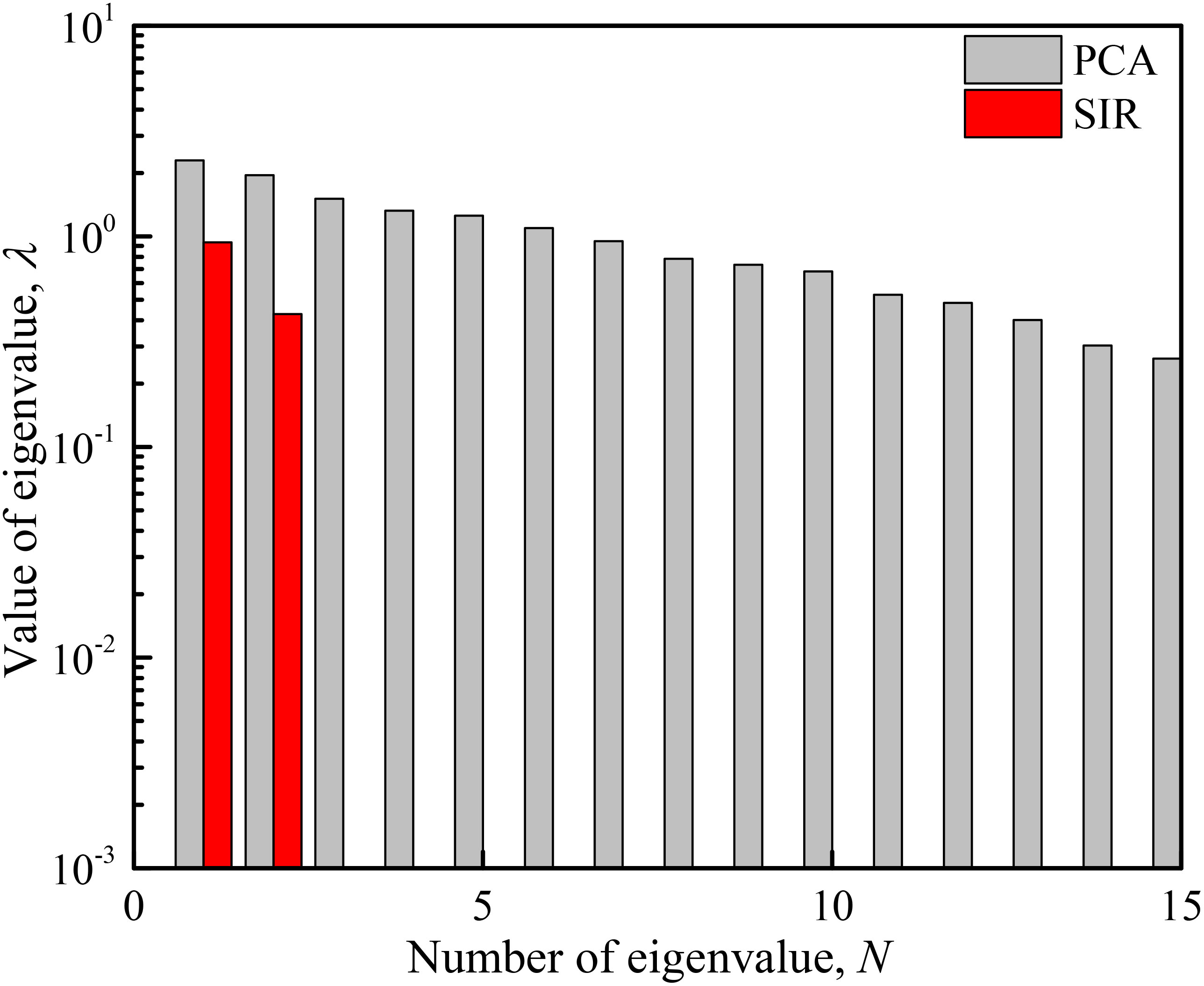
Figure 7 Comparison of the dimensionality reduction effect between PCA and SIR.
Figure 8 provides an example of one adaptive reliability analysis with the results of the updating of the cumulative distribution function, which reaches convergence after three iteration steps, with p0 = 0.1, m = 4, Nl = 5,000 in preliminary analysis and Ns = 50 in target analysis, invoking (4 + 1) × 250 + 30 = 780 FE analyses. In the first iteration, taking the first eigenvalue of λ1 and its principal direction β1 as an example, the linear combination of the first variable (ω1 = β1ξ −0.74ξ1 + 0.27ξ2 + 0.25ξ3 − 0.01ξ4 + 0.03ξ5 + 0.17ξ6 + 0.05ξ7 + 0.23ξ8 + 0.02ξ9 + 0.03ξ10 − 0.32ξ11 − 0.13ξ12 + 0.01ξ13 − 0.31ξ14 − 0.10ξ15) is the same as that of ω2. Relative to the original 15-variable RS model, it is possible to construct a more simple (only two variables) quadratic polynomial RS model in dimensionality-reduced space (Y = 0.31 + 0.08ω1 − 0.03ω2 + 0.006ω12 + 0.002ω22). Pf,RS is 0 in the preliminary reliability analysis of the first iteration, which showcases inadequate accuracy of the RS owing to the dimensionality-reduced bias in the principal direction of the SIR, resulting in that the finite number of layers of subset simulation does not reach the failure domain. Additionally, the initial correlation between FSRS and FSFE is 0.801 and the sample dispersion of the first iteration is large, specifically near the failure domain where there is a significant bias, as shown in Figure 8. Nevertheless, the introduction of representative sample points in the original space recalculated in target reliability analysis leading to an unbiased probability of 4.35 × 10⁻⁴.
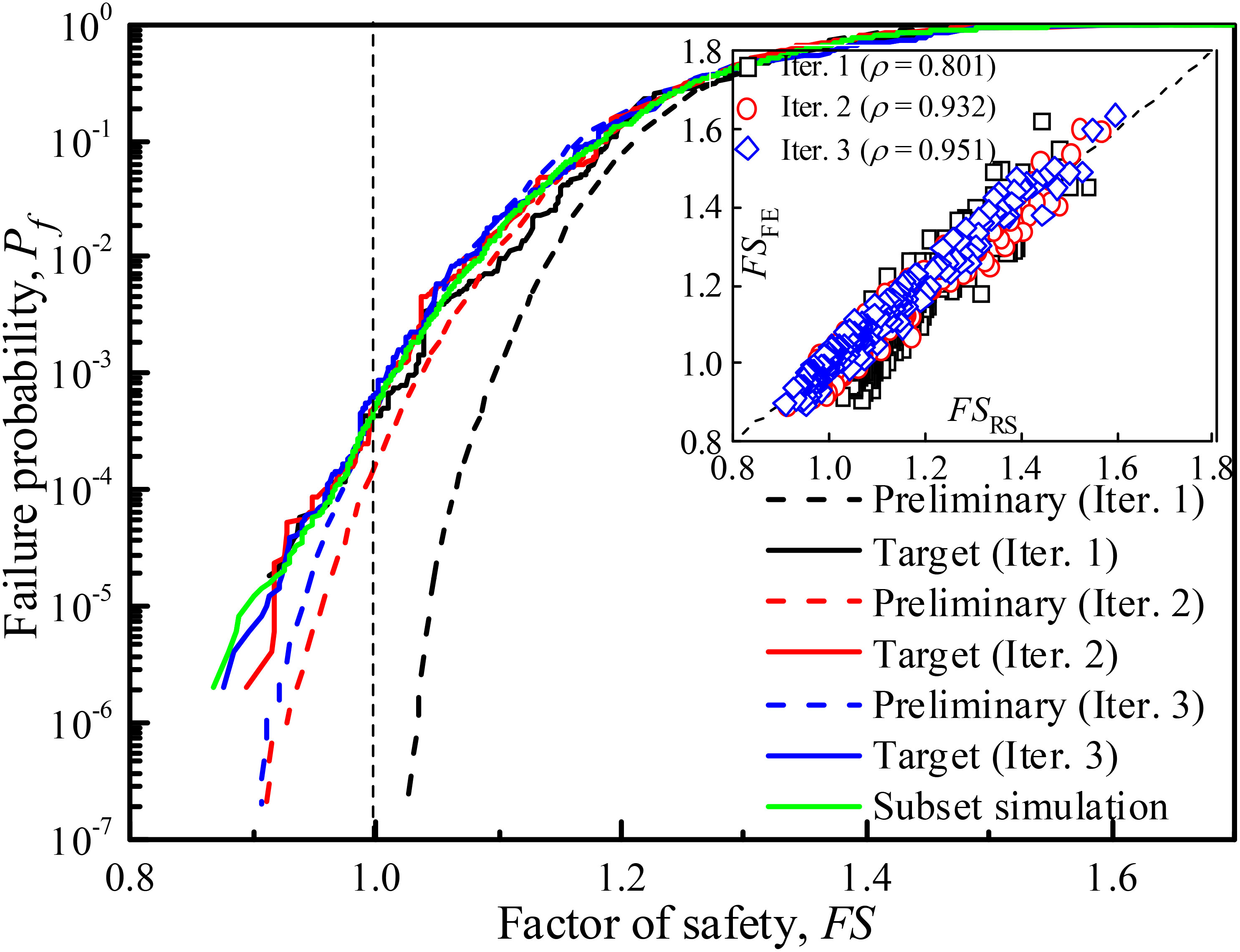
Figure 8 Updating of cumulative distribution function using adaptive reliability analysis.
Representative samples near the failure domain are appended to the training samples to update the SIR principal directions. As shown in Figure 9, the first principal direction update in iteration 2 is primarily reflected in the reduction of the weights of the 5th, 6th, 7th, and 8th random variables and the increase of the weights of the 11th, 12th, and 14th random variables. The updated RS model is obtained based on the updated principal directions as Y = 0.30 + 0.11ω1 + 0.002ω2 + 0.005ω12 + 0.001ω22 (see Figure 10). Therefore, the preliminary reliability analysis Pf,RS significantly increases to 1.66 × 10⁻⁴, which is closer to the target failure probability of this iteration step (i.e., 5.24 × 10⁻⁴). Meanwhile, the correlation coefficient increases to 0.932. The update in the principal direction of the SIR in the third iteration of the analysis is majorly reflected in the increase in the weight of first variable from a negative value to a larger positive value of 0.68, as well as the decrease in the weights of second and third variables (see Figure 9), obtaining a higher model correlation coefficient (0.951). The final reliability estimates for Pf,RS and Pf,FE are 4.98 × 10⁻⁴ and 6.58 × 10⁻⁴, respectively.
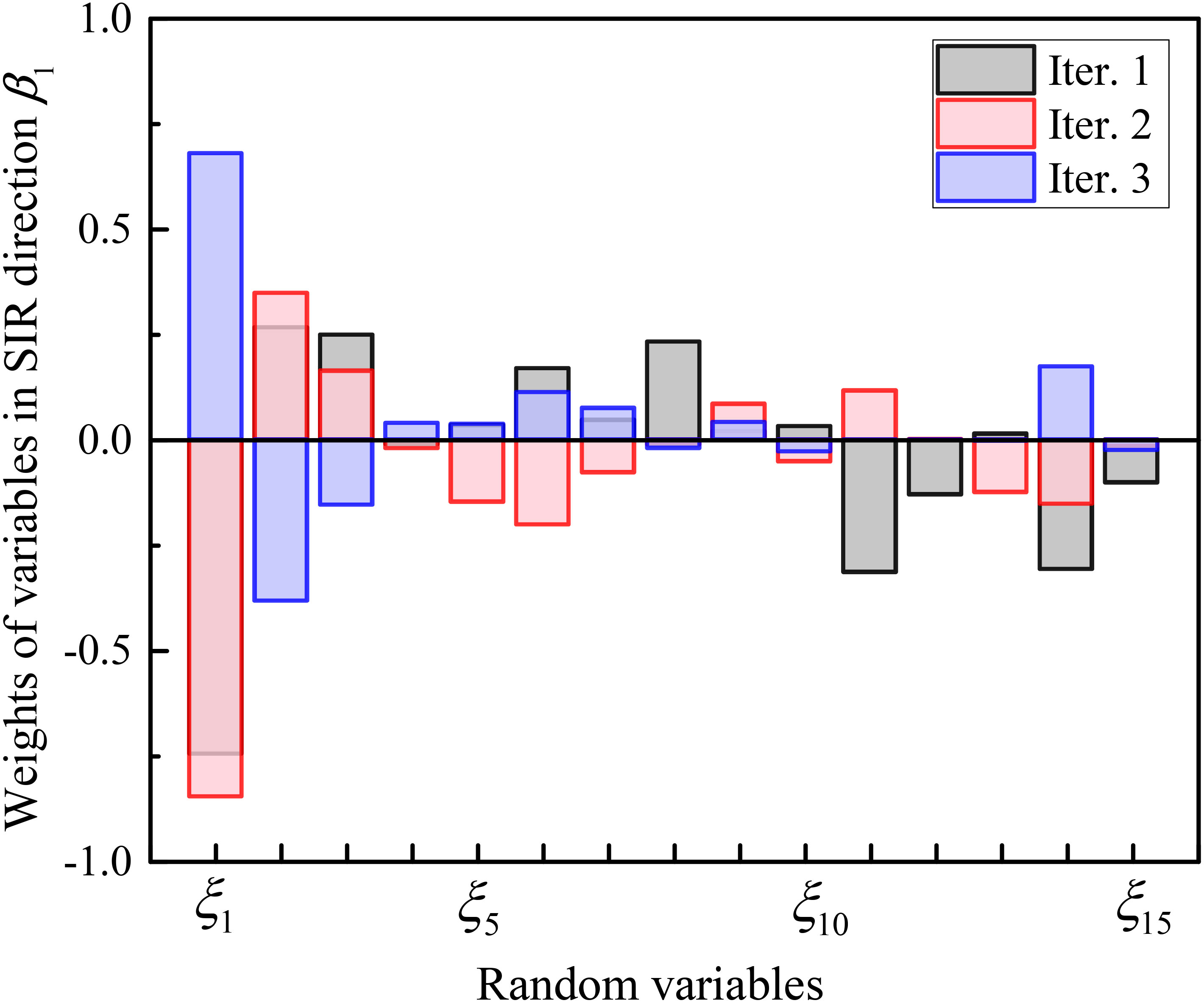
Figure 9 Updating of first SIR direction in adaptive reliability analysis.
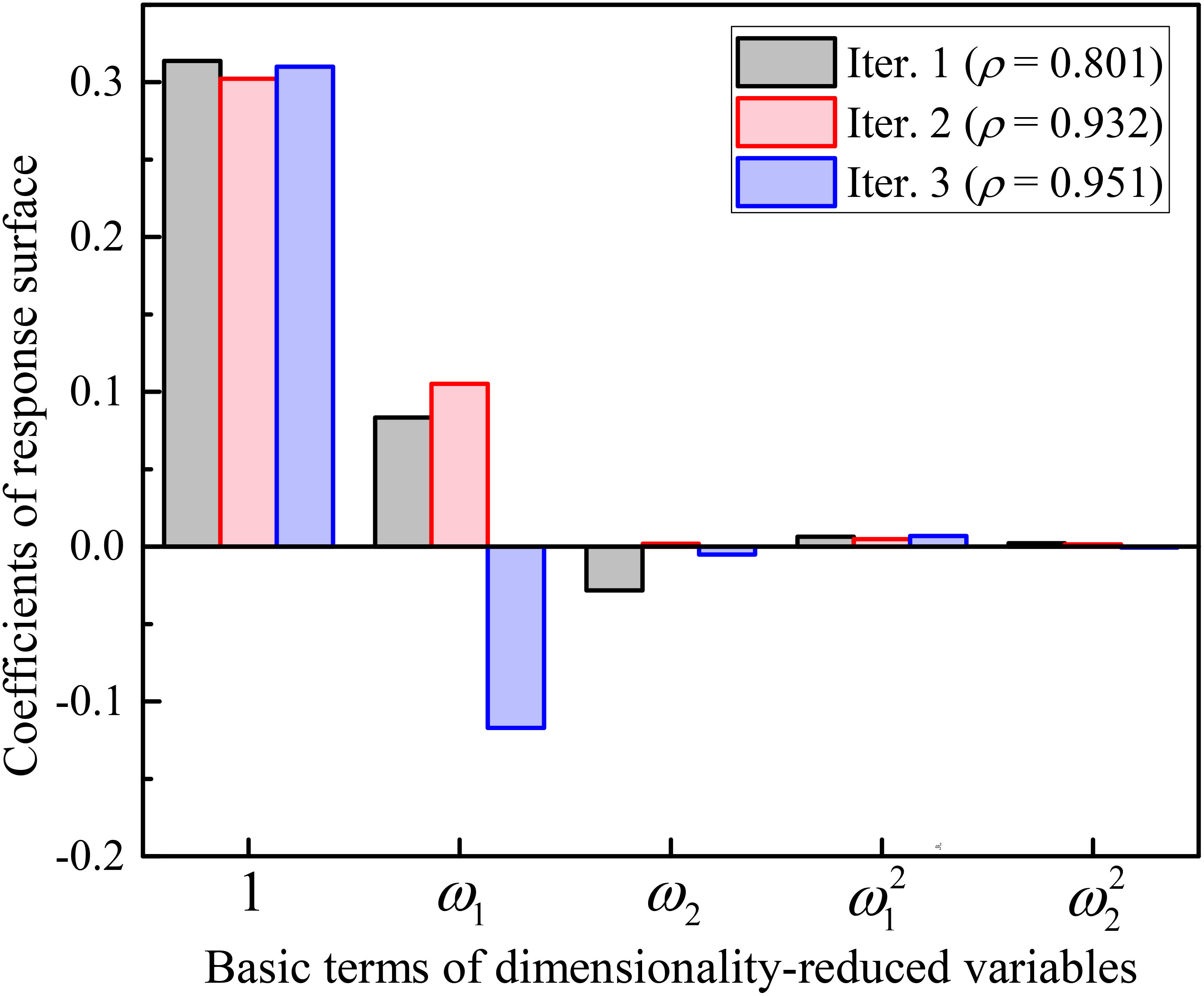
Figure 10 Updating of RS model in adaptive reliability analysis.
In addition, different sampling methods, the Monte Carlo sampling method (MCS) and Latin hypercube sampling method (LHS), are used for comparison in Table 2 and the results are basically found to be the same. The effect on the accuracy loss of the SIR dimensionality reduction process between 3,000 samples and 30 samples is also compared; it can be seen that the principal direction of the SIR obtained based on 3,000 MCS is closer to being unbiased. However, this proposed method can correct the SIR direction with only a sample size of 1/100 to obtain a consistent reliability assessment, which is also close to the subset simulation results of 1,850 FE analyses (p0 = 0.1, m = 4, and Nl = 500). In addition, to fairly compare the computational efficiency among different reliability methods, the unit COV is taken as a measurement to consider the effect of sample size on the variation of reliability estimation, calculated as COV(Pf) × Nt1/2 (Au, 2007), where Nt is the total number of FE analyses. For reference, the unit COV of the Monte Carlo simulation roughly equals to 1/Pf1/2, which is treated as the upper bound of unit COV. As shown in Table 3, the variability of the final iteration of adaptive analysis is reduced by nearly three times that in the subset simulation method, more importantly, with only around one-third computational efforts. In addition, the unit COV of adaptive analysis is 4.94, which is only one-fifth of the subset simulation method (23.66) and one-eighth of the Monte Carlo simulation method (39.99), which demonstrates that the computational efficiency of the adaptive slope reliability analysis method is increased by 25 and 64 times, respectively. Moreover, as the iterations increase, the COV(Pf,FE) in the target reliability analysis decreases from a moderate level of 0.54 to a lower level of 0.19. Furthermore, the unit COV decreases from 9.04 to 4.94, which means the adaptive process wins more variability reduction compared with the computational efforts.
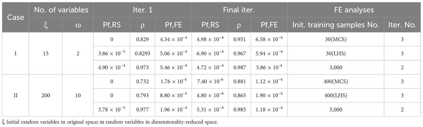
Table 2 Results of adaptive reliability analysis for the undrained slope example.
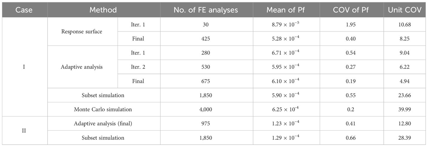
Table 3 Comparison of reliability analyses using different methods.
As previously mentioned, an increase in initial training samples N can reduce accuracy loss, and the number of dimensionality-reduced variables d can also affect the accuracy. Taking this benchmark case as an example, a sensitivity analysis is performed to explore the effects of these two parameters on the accuracy loss in the SIR dimensionality reduction process and the error correction effect of the adaptive slope reliability analysis. The effect of different values of N and d on the results of the adaptive reliability analysis method is illustrated in Table 4. Despite the large dimensionality reduction error (lower correlation coefficient of ρ) caused by the smaller number of training samples, this adaptive method can quickly improve the accuracy of failure probability to an unbiased estimation through adaptive iterations. This adaptive reliability analysis method is insensitive to parameters N and d, thereby solving the problem of parameter-dependent accuracy in SIR dimensionality reduction. This is because a large number of samples near the failure domain in the iteration step are added to the initial training samples to gradually update the principal direction of dimensionality reduction and the form of the response surface. As a suggestion for practical choice, N can be approximately taken as double the number of random variables and d can be chosen as suggested by Pan and Dias (2017).

Table 4 Impact of SIR dimensionality reduction parameters on adaptive reliability analysis.
As mentioned in the previous section, as the number of variables increases, the number training samples also increases to ensure the accuracy of the dimensionality reduction process. In this section, we investigate the effect of the proposed method in the high-dimensional case. In this case, the correlation function type is single exponential (SExp) and the number of expansion terms of K–L random field discretization is increased from 15 to 200 to achieve 95% accuracy.
Based on these 200 variables, 400 training samples are used for dimensionality reduction and 10 dimensionality-reduced variables are obtained. The adaptive reliability analysis is then performed with p0 = 0.1, m = 4, Nl = 5,000, and Ns = 50. After three iterations, the correlation between the response value of RS in the dimensionality-reduced space and the value of the FE model in the original space increases from 0.732 to 0.881. The final target failure probability is 1.12 × 10⁻⁴, which is significantly improved compared with the initial result (i.e., 0) obtained from the RS model. The procedure requires only 400 initial training samples to obtain unbiased results compared with the result of 5,000 training samples (see Table 2). As shown in Figure 11, there are still some errors with the RS model in the three iterations, but its gradual shifting toward a more accurate value and the target reliability estimates all remain within the range of reasonable values. The corresponding unit COV based on this method is one-half that of the subset simulation method and one-seventh that of the Monte Carlo simulation method (see Table 3), which shows the high effectiveness of the proposed method.
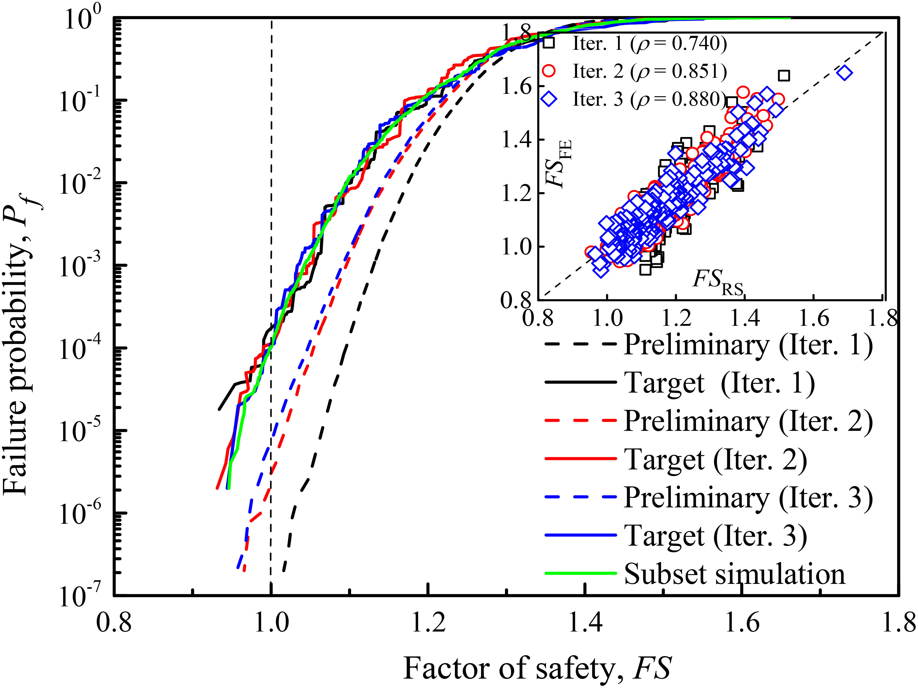
Figure 11 Results of adaptive reliability analysis in the high-dimensional case of the undrained slope example.
This adaptive slope reliability analysis method is further investigated in a more complex slope example containing a weak layer (Kim et al., 2002; Xiao et al., 2015). The slope has a height of 12.2 m, an angle of 26.6°, and a weak layer with a thickness of 0.4 m above the bedrock (see Figure 12). The geotechnical parameters of the upper and weak layers are listed in Table 5, where there are three uncertainty parameters (i.e., cohesion and friction angle of upper-layer soil c1, ϕ1, and friction angle of weak-layer soil ϕ2). The deterministic safety factor of slope stability is 1.336 through the shear strength reduction technique in FE analysis, same with Xiao et al. (2015) and between the lower and upper bounds using limit analysis (Kim et al., 2002). The spatial variability is simulated using a lognormal random field, where the type of autocorrelation function is SExp, with horizontal and vertical autocorrelation distances of 20 m and 2 m, respectively. The number of required K–L expansion terms is 910 (i.e., 440 for c1, ϕ1, 30 for ϕ2) to satisfy the accuracy of random field discretization (i.e., 95%).
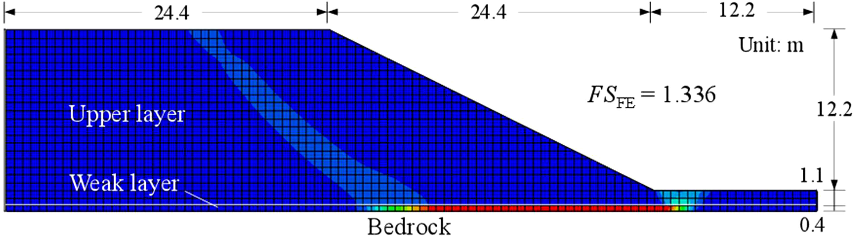
Figure 12 Deterministic FE analysis of the weak-layer slope example.
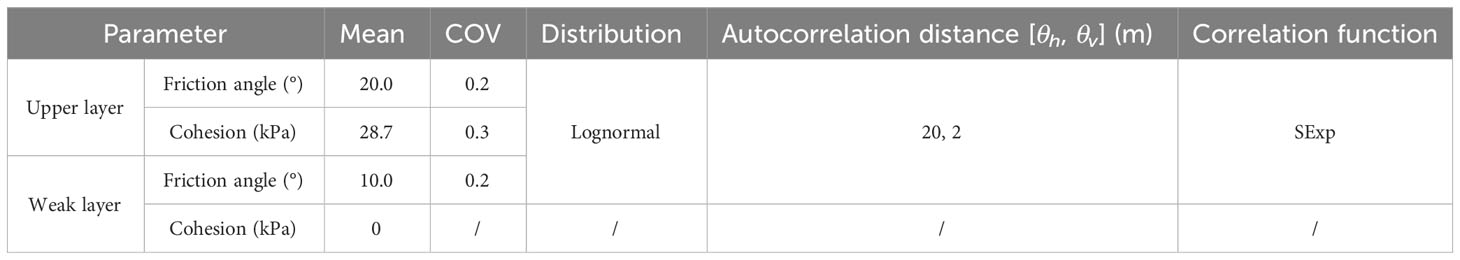
Table 5 Soil properties for the weak-layer slope example.
Because of the dimension increase of geotechnical parameters, the initial number of required training samples is appropriately increased. Taking the 2,000 training samples and 20 principal directions as an example, the initial RS in the dimensionality-reduced space is constructed. In three iterations with p0 = 0.1, m = 4, Nl = 5,000, and Ns = 50, the preliminary failure probability of RS is updated to the final reliability from 0 to 2.62 × 10⁻⁴. The correlation between the response value of RS in the dimensionality-reduced space and the response values of the FE model in the original space increased from 0.734 to 0.835. The SIR dimensionality reduction with 50,000 training samples was considered as a comparison. Although convergence is reached in two rounds with higher correlations of 0.973 and 0.975, only 1/25 of the samples is required in this adaptive analysis to obtain an unbiased reliability assessment consistent with the results of the sufficient sample (see Figure 13), which again illustrates the high effectiveness of the proposed approach.
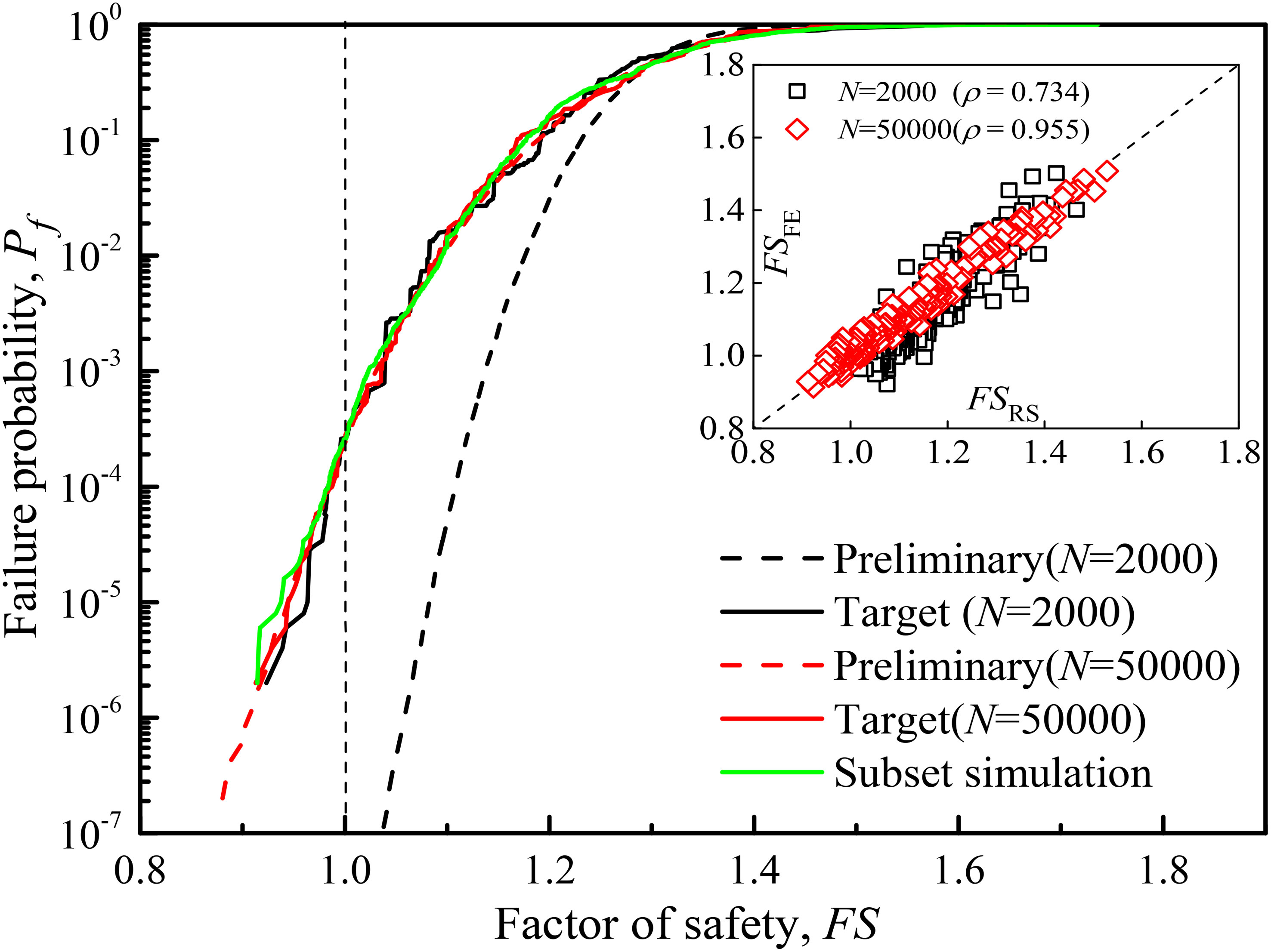
Figure 13 Results of adaptive reliability analysis in the weak-layer slope example.
In this paper, an adaptive slope reliability analysis method based on SIR dimensionality reduction is proposed. Accordingly, this method addresses the information loss problem of the SIR method through three steps: preliminary reliability analysis based on the subset simulation of the RS model in the dimensionality-reduced space, target reliability analysis based on the finite-element model and response condition method in the original space, and adaptive strategy of the SIR principal direction and RS updating. Two spatial variability slopes were used to verify the effectiveness of the proposed method. The main conclusions are as follows.
(1) The effects of dimensionality reduction between PCA and SIR methods considering spatially varying soils were compared in slope reliability analysis. Taking advantage of the relationship between input and response variables in the SIR method, it is easier to determine larger direction vectors for dimensionality reduction. In addition, in this paper, the initial training samples can be repeatedly used as response surface training samples to reduce the computational cost. However, the accuracy of SIR dimensionality reduction is affected by the parameters; a large loss of information will be induced specifically when the number of training samples is limited.
(2) The proposed adaptive reliability analysis method reduces the requirement of determining a highly correlated simple model in the response conditioning method, and the accuracy requirement of the initial principal direction of dimensionality reduction, thus overcoming the information loss of the traditional SIR dimensionality reduction method. The correlation between the dimensionality-reduced space and the original space was also utilized to update the principal direction of SIR dimensionality reduction and the response surface model by adding the original space training samples near the failure domain.
(3) The adaptive slope reliability analysis method has a suitable correction effect on the SIR dimensionality reduction error in various dimensions for both single-layer slopes and relatively complex slopes containing a weak layer. The proposed method significantly improves the computational efficiency compared with the traditional SIR method, subset simulation method, and Monte Carlo method, it can obtain stable and unbiased slope reliability assessment with a small number of samples, thereby enhancing the application of RS in slope reliability analysis considering the curse of high dimensionality.
The original contributions presented in the study are included in the article/supplementary material. Further inquiries can be directed to the corresponding author.
ZZ: Conceptualization, Investigation, Methodology, Software, Validation, Writing – original draft, Writing – review & editing. H-BX: Software, Validation, Writing – original draft. W-XW: Validation, Writing – original draft. Y-JY: Validation, Writing – review & editing. X-HY: Supervision, Validation, Writing – review & editing.
The authors declare that no financial support was received for the research, authorship, and/or publication of this article.
Authors ZZ, H-BX, W-XW, and Y-JY were employed by the company Changjiang Survey, Planning, Design and Research Co., Ltd.
The remaining author declares that the research was conducted in the absence of any commercial or financial relationships that could be construed as a potential conflict of interest.
All claims expressed in this article are solely those of the authors and do not necessarily represent those of their affiliated organizations, or those of the publisher, the editors and the reviewers. Any product that may be evaluated in this article, or claim that may be made by its manufacturer, is not guaranteed or endorsed by the publisher.
Al-Bittar T., Soubra A. H. (2014). Efficient sparse polynomial chaos expansion methodology for the probabilistic analysis of computationally-expensive deterministic models. Int. J. Numer. Anal. Meth. Geomech. 38 (12), 1211–1230.
Au S. K. (2007). Augmenting approximate solutions for consistent reliability analysis. Probabilistic Eng. Mech. 22 (1), 77–87.
Au S. K., Beck J. L. (2001). Estimation of small failure probabilities in high dimensions by Subset Simulation. Probabilistic Eng. Mech. 16 (4), 263–277.
Blatman G., Sudret B. (2010). An adaptive algorithm to build up sparse polynomial chaos expansions for stochastic finite element analysis. Probabilistic Eng. Mech. 25 (2), 183–197.
Blatman G., Sudret B. (2011). Adaptive sparse polynomial chaos expansion based on least angle regression. J. Comput. Phys. 230 (6), 2345–2367.
Bucher C. G., Bourgund U. (1990). A fast and efficient response surface approach for structural reliability problems. Struct. Saf. 7 (1), 57–66.
Cao Z. J., Zheng S., Li D. Q., Phoon K. K. (2019). Bayesian identification of soil stratigraphy based on soil behaviour type index. Can. Geotech. J. 56 (4), 570–586.
Chang Z., Du Z., Zhang F., Huang F., Chen J., Li W., et al. (2020). Landslide susceptibility prediction based on remote sensing images and GIS: comparisons of supervised and unsupervised machine learning models. Remote Sensing. 12, 502.
Cheng K., Lu Z. Z. (2018). Adaptive sparse polynomial chaos expansions for global sensitivity analysis based on support vector regression. Comput. Struct. 194, 86–96.
Cho S. E. (2007). Effects of spatial variability of soil properties on slope stability. Eng. Geol. 92 (3), 97–109.
Cho S. E. (2009). Probabilistic stability analyses of slopes using the ANN-based response surface. Comput. Geotech. 36 (5), 787–797.
Cho S. E. (2010). Probabilistic assessment of slope stability that considers the spatial variability of soil properties. J. Geotech. Geoenviron. 136 (7), 975–984.
Christian J. T., Ladd C. C., Baecher G. B. (1994). Reliability applied to slope stability analysis. J. Geotech. Eng. 120 (12), 2180–2207.
Constantine P. G., Dow E., Wang Q. (2014). Active subspace methods in theory and practice: applications to kriging surfaces. SIAM. J. Sci. Comput. 36 (4), A1500–A1524.
Deng Z. P., Jiang S. H., Niu J. T. (2020). Stratigraphic uncertainty characterization using modified generalized coupled Markov chain. Bull. Eng. Geology Environ. 79, 5061–5078.
Deng Z. P., Li D. Q., Qi X. H., Cao Z. J., Phoon K. K. (2017). Reliability evaluation of slope considering geological uncertainty and inherent variability of soil parameters. Comput. Geotechnics 92 (C), 121–131.
Deng Z. P., Pan M., Niu J. T., Jiang S. H. (2022). Full probability design of soil slopes considering both stratigraphic uncertainty and spatial variability of soil properties. Bull. Eng. Geology Environment. 81 (5), 1–13.
Deng Z. P., Pan M., Niu J. T., Jiang S. H., Qian W. W. (2021). Slope reliability analysis in spatially variable soils using sliced inverse regression-based multivariate adaptive regression spline. Bull. Eng. Geology Environmen 80 (9), 7213–7226.
Dubourg V., Sudret B., Deheeger F. (2013). Metamodel-based importance sampling for structural reliability analysis. Probabilistic Eng. Mech. 33, 47–57.
Echard B., Gayton N., Lemaire M. (2011). AK-MCS: an active learning reliability method combining Kriging and Monte Carlo simulation. Struct. Saf. 33 (2), 145–154.
Griffiths D. V., Fenton G. A. (2004). Probabilistic slope stability analysis by finite elements. J. Geotech. Geoenviron. Eng. 130 (5), 507–518.
Guimarães H., Matos J. C., Henriques A. A. (2018). An innovative adaptive sparse response surface method for structural reliability analysis. Struct. Saf. 73, 12–28.
Hassan A. M., Wolff T. F. (1999). Search algorithm for minimum reliability index of earth slopes. J. Geotech. Geoenviron. 125 (4), 301–308.
Huang F. M., Cao Z. S., Guo J. F., Jiang S. H., Guo Z. Z. (2020a). Comparisons of heuristic, general statistical and machine learning models for landslide susceptibility prediction and mapping. CATENA. 191, 104580.
Huang F. M., Cao Z. S., Jiang S. H., Zhou C. B., Guo Z. Z. (2020b). Landslide susceptibility prediction based on a semi-supervised multiple-layer perceptron model. Landslides. 17, 2919–2930.
Huang J. S., Griffiths D. V., Fenton G. A. (2010). System reliability of slopes by RFEM. Soils Found. 50 (3), 343–353.
Huang J., Lyamin A. V., Griffiths D. V., Krabbenhoft K., Sloan S. W. (2013). Quantitative risk assessment of landslide by limit analysis and random fields. Comput. Geotech. 53, 60–67.
Huang F. M., Zhang J., Zhou C. B., Wang Y. H., Huang J. S., Zhu L. (2020c). A deep learning algorithm using a fully connected sparse autoencoder neural network for landslide susceptibility prediction. Landslides 17 (01), 217–229.
Ji J. (2014). A simplified approach for modeling spatial variability of undrained shear strength in out-plane failure mode of earth embankment. Eng. Geol. 183, 315–323.
Ji J., Liao H. J., Low B. K. (2012). Modeling 2-D spatial variation in slope reliability analysis using interpolated autocorrelations. Comput. Geotech. 40, 135–146.
Ji J., Low B. K. (2012). Stratified response surfaces for system probabilistic evaluation of slopes. J. Geotech. Geoenviron. Eng. 138 (11), 1398–1406.
Jiang S. H., Huang J., Huang F. M., Yang J. H., Yao C., Zhou C. B. (2018). Modelling of spatial variability of soil undrained shear strength by conditional random fields for slope reliability analysis. Appl. Math. Model. 63, 374–389.
Jiang S. H., Li D. Q., Cao Z. J., Zhou C. B., Phoon K. K. (2015). Efficient system reliability analysis of slope stability in spatially variable soils using Monte Carlo simulation. J. Geotech. Geoenviron. Eng. 141 (2), 04014096.
Jiang S. H., Li D. Q., Zhang L. M., Zhou C. B. (2014). Slope reliability analysis considering spatially variable shear strength parameters using a non-intrusive stochastic finite element method. Eng. Geol. 168, 120–128.
Kim J., Salgado R., Lee J. (2002). Stability analysis of complex soil slopes using limit analysis. J. Geotech. Geoenviron. Eng. 128 (7), 546–557.
Li K. C. (1991). Sliced inverse regression for dimension reduction. J. Am. Stat. Assoc., 86, 316–342.
Li C. C., Der Kiureghian A. (1993). Optimal discretization of random fields. J. Eng. Mech. 119 (6), 1136–1154.
Li D. Q., Jiang S. H., Cao Z. J., Zhou W., Zhou C. B., Zhang L. M. (2015a). A multiple response-surface method for slope reliability analysis considering spatial variability of soil properties. Eng. Geol. 187, 60–72.
Li W., Lin G., Li B. (2016c). Inverse regression-based uncertainty quantification algorithms for high-dimensional models: Theory and practice. J. Comput. Phys. 321, 259–278.
Li D. Q., Tang X. S., Phoon K. K. (2015b). Bootstrap method for characterizing the effect of uncertainty in shear strength parameters on slope reliability. Reliab. Eng. Syst. Saf. 140, 99–106.
Li D. Q., Xiao T., Cao Z. J., Phoon K. K., Zhou C. B. (2016a). Efficient and consistent reliability analysis of soil slope stability using both limit equilibrium analysis and finite element analysis. Appl. Math. Model. 40, 5216–5229.
Li D. Q., Xiao T., Cao Z. J., Zhou C. B., Zhang L. M. (2016b). Enhancement of random finite element method in reliability analysis and risk assessment of soil slopes using Subset Simulation. Landslides 13, 293–303.
Li D. Q., Xiao T., Zhang L. M., Cao Z. J. (2019a). Stepwise covariance matrix decomposition for efficient simulation of multivariate large-scale three-dimensional random fields. Appl. Math. Model. 68, 169–181.
Li S. J., Zhao H. B., Ru Z. L. (2013). Slope reliability analysis by updated support vector machine and Monte Carlo simulation. Nat. Hazards 65 (1), 707–722.
Li D. Q., Zheng D., Cao Z. J., Tang X. S., Qi X. H. (2019b). Two-stage dimension reduction method for meta-model based slope reliability analysis in spatially variable soils. Struct. Saf. 81, 101872.
Liu X., Wang Y., Li D. Q. (2019). Investigation of slope failure mode evolution during large deformation in spatially variable soils by random limit equilibrium and material point methods. Comput. Geotech. 111, 301–312.
Low B. K. (2014). FORM, SORM, and spatial modeling in geotechnical engineering. Struct. Saf. 49, 56–64.
Low B. K., Tang W. H. (1997). Probabilistic slope analysis using Janbu's generalized procedure of slices. Comput. Geotech. 21 (2), 121–142.
Low B. K., Tang W. H. (2004). Reliability analysis using object-oriented constrained optimization. Struct. Saf. 26 (1), 69–89.
Luo X. F., Cheng T., Li X., Zhou J. (2012a). Slope safety factor search strategy for multiple sample points for reliability analysis. Eng. Geol. 129, 27–37.
Luo X. F., Li X., Zhou J., Cheng T. (2012b). A Kriging-based hybrid optimization algorithm for slope reliability analysis. Struct. Saf. 34 (1), 401–406.
Marelli S., Sudret B. (2018). An active-learning algorithm that combines sparse polynomial chaos expansions and bootstrap for structural reliability analysis. Struct. Saf. 11, 67–74.
Nie J., Cui Y. F., Senetakis K., Guo D., Wang Y., Wang G. D., et al. (2023). Predicting residual friction angle of lunar regolith based on Chang'e-5 lunar samples. Sci. Bull. 68 (7), 730–739.
Pan Q., Dias D. (2017). Sliced inverse regression-based sparse polynomial chaos expansions for reliability analysis in high dimensions. Reliab. Eng. Syst. Saf. 167, 484–493.
Peng J., Hampton J., Doostan A. (2014). A weighted 𝓁1-minimization approach for sparse polynomial chaos expansions. J. Comput. Phys. 267, 92–111.
Phoon K. K., Huang S. P., Quek S. T. (2002). Implementation of Karhunen–Loeve expansion for simulation using a wavelet-Galerkin scheme. Probabilistic Eng. Mech. 17 (3), 293–303.
Piliounis G., Lagaros N. D. (2014). Reliability analysis of geostructures based on metaheuristic optimization. Appl. Soft Comput. 22, 544–565.
Tan X. H., Bi W. H., Hou X. L., Wang W. (2011). Reliability analysis using radial basis function networks and support vector machines. Comput. Geotech. 38 (2), 178–186.
Tan X. H., Shen M. F., Hou X. L., Li D., Hu N. (2013). Response surface method of reliability analysis and its application in slope stability analysis. Geotech. Geol. Eng. 31 (4), 1011–1025.
Varkey D., Hicks M. A., Vardon P. J. (2019). An improved semi-analytical method for 3D slope reliability assessments. Comput. Geotech. 111, 181–190.
Wang Y., Cao Z. J., Au S. K. (2010). Efficient Monte Carlo simulation of parameter sensitivity in probabilistic slope stability analysis. Comput. Geotech. 37 (7), 1015–1022.
Wang Y., Cao Z. J., Au S. K. (2011). Practical reliability analysis of slope stability by advanced Monte Carlo simulations in a spreadsheet. Can. Geotech. J. 48, 162–172.
Wang L., Wu C., Gu X., Liu H., Mei G., Zhang W. (2020a). Probabilistic stability analysis of earth dam slope under transient seepage using multivariate adaptive regression splines. Bull. Eng. Geol. Environ. 79 (6), 2763–2775.
Wang L., Wu C., Tang L., Zhang W., Lacasse S., Liu H., et al. (2020b). Efficient reliability analysis of earth dam slope stability using extreme gradient boosting method. Acta Geotech. 15 (11), 3135–3150.
Xiao T., Li D. Q., Cao Z. J., Au S. K., Phoon K. K. (2016). Three-dimensional slope reliability and risk assessment using auxiliary random finite element method. Comput. Geotech. 79, 146–158.
Xiao T., Li D. Q., Cao Z. J., Tang X. S. (2015). Non-intrusive reliability analysis of multi-layered slopes in spatially variable soils. In fifth International Symposium on Geotechnical Safety and Risk (ISGSR 2015), Rotterdam, The Netherlands, October 13-16, 2015. Geotechnical Safety and Risk V, Schweckendiek T., et al (Eds.), pp 184–190.
Xiao T., Li D. Q., Cao Z. J., Tang X. S. (2017). Full probabilistic design of slopes in spatially variable soils using simplified reliability analysis method. Georisk 11 (1), 146–159.
Xiao T., Li D. Q., Cao Z. J., Zhang L. M. (2018). CPT-based probabilistic characterization of three-dimensional spatial variability using MLE. J. Geotech. Geoenviron. Eng. 144 (5), 04018023.
Xu B., Low B. K. (2006). Probabilistic stability analyses of embankments based on finite element method. J. Geotech. Geoenviron. 132 (11), 1444–1145.
Xue J. F., Gavin K. (2007). Simultaneous determination of critical slip surface and reliability index for slopes. J. Geotech. Geoenviron. 133 (7), 878–886.
Yang X., Lei H., Baker N. A., Lin G. (2016). Enhancing sparsity of Hermite polynomial expansions by iterative rotations. J. Comput. Phys. 307, 94–109.
Zeng P., Jimenez R. (2014). An approximation to the reliability of series geotechnical systems using a linearization approach. Comput. Geotech. 62, 304–309.
Zhang L., Cui Y., Zhu H. H., Wu H., Han H., Yan Y., et al. (2023a). Shear deformation calculation of landslide using distributed strain sensing technology considering the coupling effect. Landslides 20 (8), 1583–1597. doi: 10.1007/s10346-023-02051-5
Zhang W., Gu X., Hong L., Han L., Wang L. (2023c). Comprehensive review of machine learning in geotechnical reliability analysis: Algorithms, applications and further challenges. Appl. Soft Computing 136, 110066.
Zhang J., Huang H. W., Phoon K. K. (2013). Application of the Kriging-based response surface method to the system reliability of soil slopes. J. Geotech. Geoenviron. Eng. 139 (4), 651–655.
Zhang L., Zhu H. H., Han H. M., Shi B. (2023b). Fiber optic monitoring of an anti-slide pile in a retrogressive landslide. J. Rock Mechanics Geotechnical Eng. doi: 10.1016/j.jrmge.2023.02.011
Zhou Z., Li D. Q., Xiao T., Cao Z. J., Du W. Q. (2021). Response surface guided adaptive slope reliability analysis in spatially varying soils. Comput. Geotech. 132 (12), 103966. doi: 10.1016/j.compgeo.2020.103966
Keywords: spatial variability, sliced inverse regression, response surface, subset simulation, response conditioning method
Citation: Zhou Z, Xiong H-B, Wu W-X, Yang Y-J and Yang X-H (2023) Adaptive slope reliability analysis method based on sliced inverse regression dimensionality reduction. Front. Ecol. Evol. 11:1257854. doi: 10.3389/fevo.2023.1257854
Received: 13 July 2023; Accepted: 29 August 2023;
Published: 22 September 2023.
Edited by:
Faming Huang, Nanchang University, ChinaReviewed by:
Bin Guo, Cardiff University, United KingdomCopyright © 2023 Zhou, Xiong, Wu, Yang and Yang. This is an open-access article distributed under the terms of the Creative Commons Attribution License (CC BY). The use, distribution or reproduction in other forums is permitted, provided the original author(s) and the copyright owner(s) are credited and that the original publication in this journal is cited, in accordance with accepted academic practice. No use, distribution or reproduction is permitted which does not comply with these terms.
*Correspondence: Xu-Hai Yang, eXh1aGFpQDE2My5jb20=
Disclaimer: All claims expressed in this article are solely those of the authors and do not necessarily represent those of their affiliated organizations, or those of the publisher, the editors and the reviewers. Any product that may be evaluated in this article or claim that may be made by its manufacturer is not guaranteed or endorsed by the publisher.
Research integrity at Frontiers
Learn more about the work of our research integrity team to safeguard the quality of each article we publish.