Monitoring marine pollution for carbon neutrality through a deep learning method with multi-source data fusion

Introduction: Marine pollution can have a significant impact on the blue carbon, which finally affect the ocean’s ability to sequester carbon and contribute to achieving carbon neutrality. Marine pollution is a complex problem that requires a great deal of time and effort to measure. Existing machine learning algorithms cannot effectively solve the detection time problem and provide limited accuracy. Moreover, marine pollution can come from a variety of sources. However, most of the existing research focused on a single ocean indicator to analyze marine pollution. In this study, two indicators, marine organisms and debris, are used to create a more complete picture of the extent and impact of pollution in the ocean.

Methods: To effectively recognize different marine objects in the complex marine environment, we propose an integrated data fusion approach where deep convolutional neural networks (CNNs) are combined to conduct underwater object recognition. Through this multi-source data fusion approach, the accuracy of object recognition is significantly improved. After feature extraction, four machine and deep learning classifiers’ performances are used to train on features extracted with deep CNNs.

Results: The results show that VGG-16 achieves better performance than other feature extractors when detecting marine organisms. When detecting marine debris, AlexNet outperforms other deep CNNs. The results also show that the LSTM classifier with VGG-16 for detecting marine organisms outperforms other deep learning models.

Discussion: For detecting marine debris, the best performance was observed with the AlexNet extractor, which obtained the best classification result with an LSTM. This information can be used to develop policies and practices aimed at reducing pollution and protecting marine environments for future generations.

1 Introduction

Marine pollution and carbon neutrality have commonly been treated as two separate issues. The research articles simultaneously examining marine pollution and carbon neutrality are few. Here, we present an alternative view that these two issues are fundamentally linked. It is widely known that both marine pollution and carbon neutrality are linked to blue carbon. Marine pollution has a significant impact on blue carbon (Moraes, 2019). Blue carbon is important for achieving carbon neutrality as it provides a valuable opportunity for carbon sequestration (Zhu and Yan, 2022). Therefore, reducing marine pollution, directly or indirectly, protects blue carbon, thereby achieving carbon neutrality. To achieve carbon neutrality, monitoring and addressing marine pollution are important. There are several common ocean indicators that should always be used to monitor marine pollution: marine organisms (Theerachat et al., 2019), marine debris (Ryan et al., 2020), oil spill (Jiao et al., 2019), chlorophyll-a concentration (Franklin et al., 2020), dissolved oxygen (Hafeez et al., 2018), and the pH of seawater (El Zrelli et al., 2018). Most of the existing research focused on a single ocean indicator to monitor marine pollution. To better monitor marine pollution, two ocean indicators have been introduced in this study. Marine organisms and marine debris are selected to monitor marine pollution. Specifically, detecting marine organisms is important for understanding the effects of pollution on marine ecosystems. Chemical contaminants are the main sources of marine pollution, resulting from the nutrient runoff of chemicals into waterways (Thompson and Darwish, 2019). It can harm the health of marine organisms and reduce their ability to take up carbon dioxide and sequester it in the ocean. To monitor chemical contaminants in the marine environment, marine organisms are selected as one of the ocean indicators. It is considered an indirect way to monitor marine pollution. On the other hand, marine debris, such as plastics, fishing gear, and other human-made materials, can harm marine life, disrupt food webs, and damage habitats. It can negatively impact the productivity and resilience of blue carbon ecosystems, reducing their ability to sequester carbon (Duan et al., 2020). Also, the production and disposal of marine debris can contribute to greenhouse gas emissions, which finally weakens carbon neutrality capacity (Lincoln et al., 2022). Thus, selecting marine debris as the other ocean indicator is considered the most direct measure of success in the campaign against marine pollution.

To detect marine debris and marine organisms, underwater object recognition, an emerging technology, is used in this study. With the help of an autonomous underwater vehicle, underwater objects can be recognized from an image and captured and analyzed to detect and identify marine organisms and marine debris (Ahn et al., 2018; Chin et al., 2022). Generally, underwater object recognition consists of two important steps, which are feature extraction and classification (Wang et al., 2022). Compared with the step of classification, feature extraction is more important and difficult because of the complexity of the marine environment. Previous research pointed out that feature extraction is a challenging task in underwater object recognition that requires efficiency and accurate object identification for marine big data processing. To date, machine learning and deep learning methods, such as MLP, RNN, and KNN, have been introduced for underwater object recognition. But the main problem is the inaccurate extraction of features, which leads to low accuracy of classifiers. A deep convolutional neural network (deep CNN) provides new possibilities for effective recognition of objects and performs better in feature extraction than most machine and deep learning methods (Chin et al., 2022). But as marine objects may have a similar color, shape, and texture, these existing methods are hardly effective in recognizing differences between marine objects. Thus, our proposed method introduces an integrated data fusion approach where a deep CNN is combined to conduct underwater object recognition. By leveraging this multi-source data fusion approach, we significantly improve the accuracy of object recognition, particularly when dealing with similar marine objects that share the same color, shape, and texture. This advanced deep learning technique ensures a more comprehensive and accurate assessment of marine pollution by effectively capturing the distinguishing features of marine organisms and debris. Furthermore, our proposed method goes beyond conventional approaches by employing specialized training strategies to enhance the performance of the deep CNN. We incorporate techniques like data augmentation to address the challenges associated with limited underwater training data and variations in marine pollution scenarios. By effectively augmenting the training data, we improve the network’s ability to generalize and recognize diverse instances of marine objects, leading to superior performance compared to existing approaches. The combination of our integrated data fusion approach and specialized training strategies enables our method to overcome the limitations of traditional feature-based methods and achieve notable advancements in underwater object recognition for marine pollution assessment. Therefore, by combining feature extraction and classification methods with multisource data fusion, our study aims to leverage the strengths of each data source and achieve a more comprehensive understanding of the marine environment’s pollution levels. This integrated approach can potentially provide valuable insights for assessing the effectiveness of carbon neutrality efforts and informing decision-making processes related to environmental management.

The contributions of this paper are:

1. We adopted multi-source based data fusion and deep CNN models together to conduct underwater object recognition. By fusing information from multiple sources and leveraging the power of deep CNNs for feature extraction and classification, the approach overcomes the limitations of using a single data source and achieves higher accuracy in identifying marine organisms and debris. This advancement is crucial for effective monitoring and mitigation of marine pollution.

2. The second contribution of this work attempts to develop a hybrid deep learning model that consists of deep CNN extractors with AI algorithm for marine object recognition, which monitoring marine pollution. This model combines the strengths of different deep learning architectures or techniques to improve the accuracy and robustness of marine object recognition. By leveraging the complementary features and capabilities of multiple deep learning approaches, the hybrid model offers enhanced performance in identifying and classifying marine objects.

3. Our paper specifically contributes by integrating two distinct ocean indicators, namely marine organisms and debris, in the data fusion process. This integration provides a more comprehensive and accurate assessment of marine pollution, surpassing the limitations of considering a single indicator alone.

4. The findings and techniques presented in our paper have practical implications for addressing marine pollution and achieving carbon neutrality. By accurately detecting and monitoring marine pollution indicators through data fusion and deep CNNs, our research contributes to the development of effective policies and practices for reducing pollution and protecting marine environments. This has long-term benefits for carbon neutrality and the preservation of marine ecosystems.

The rest of the paper is organized as follows: We provide a literature review about underwater object recognition and its related deep learning methods in Section 2. Section 3 provides details of methodology. In Section 4, the results of the experimentation are described and conducted to evaluate the performance of the proposed model. Finally, conclusions and limitations are presented.

2 Related work

2.1 Underwater object recognition

Underwater object recognition is important for a variety of applications, such as search and rescue operations, archaeological exploration, environmental monitoring, and military operations (Wang et al., 2022). By identifying and locating objects in marine environments, these technologies can increase safety, protect the environment, and advance scientific knowledge. Due to the numerous advantages of underwater object recognition, the development of techniques for underwater object detection and recognition has attracted great research efforts. Computer vision techniques are widely used to automatically detect underwater objects. Around three decades ago, stereo photographic methods were utilized to detect the locations and sizes of sharks in marine environments (Klimley and Brown, 1983). Walther et al. (2004) designed an automated system that is used by remotely operated underwater vehicles (ROVs) to detect and track underwater objects in the marine environment. Later, a trawl-based underwater camera system using an automatic segmentation algorithm for fish acquired was developed, which overcomes the low brightness contrast problem in the underwater environment (Chuang et al., 2011). However, these traditional techniques rely heavily on man-made discriminant features, which are not able to recognize various objects with similar colors, shapes, and textures in complex marine environments. With the increasing availability of data and the development of machine learning algorithms, there has been a surge in the use of machine learning and deep learning methods for object recognition in remote sensing. Researchers have explored and implemented various advanced deep networks to tackle the challenges associated with image analysis. Hong et al. (2020a) developed a new minibatch graph convolutional network (GCN) that has the ability to infer and classify out-of-sample data without requiring the retraining of networks, thus enhancing the classification performance. Meng et al. (2017) proposed a fully connected network called FCNet that uses deep features to improve the classification performance of images. Furthermore, Hong et al. (2020b) introduced a comprehensive multimodal deep learning framework called MDL-RS (Multimodal Deep Learning for Remote Sensing Imagery Classification). The primary objective of MDL-RS is to address the challenges of remote sensing (RS) image classification. The framework combines pixel-level labeling guided by an FC net design with spatial-spectral joint classification using a CNN-dominated architecture. By integrating these approaches, MDL-RS aims to achieve a unified and effective solution for RS image classification. Li et al. (2023) applied sparse neural network embedding to showcase the scalability of the LRR-Net framework. The proposed approach is evaluated on eight distinct datasets, demonstrating its effectiveness and superiority compared to state-of-the-art methods for hyperspectral anomaly detection. Recently, vision transformer (ViT) can capture global interactions between different patches in the image, enabling it to learn long range dependencies, thereby yielding higher classification performance (Bazi et al., 2021). While ViT has achieved impressive results in image classification tasks, it suffers from high computational requirements and struggles with capturing fine-grained spatial information due to the fixed-size patches used in the model. EViT builds upon the foundation of ViT to overcome Vit limitations, yielding state-of-the-art performance (Yao et al., 2023). Additionally, a multimodal fusion transformer (MFT) network is developed based on ViT to achieve better generalization (Roy et al., 2023). Similarly, in the marine environment field, most of researchers have begun to use deep learning methods to tackle their problem of identifying objects in marine environment, which finally achieved significant success. From the above discussion, the following section briefly reviews the related works and presents the development of marine organism detection and deep learning methods and the development of marine debris detection and deep CNN models.

2.2 Marine organism detection and deep learning methods

Marine organism detection is an emerging field that involves using technology and artificial intelligence to identify and classify marine organisms in underwater environments (Zhang et al., 2021). However, it is difficult to obtain sufficient marine organism data in underwater environments. Until 2018, the public datasets for deep-sea marine organisms were provided by the Japan Agency for Marine-Earth Science and Technology (JAMSTEC). Thus, there had been few attempts to apply deep learning to marine organism detection before 2018. Lu et al. (2018) used the filtering deep convolutional network (FDCNet) classifier to identify the most relevant features. The results showed that FDCNet outperformed several other state-of-the-art deep learning architectures, including ResNet, VGG-16, and InceptionNet, achieving an accuracy of over 98%. Huang et al. (2019) first introduced deep convolutional networks to marine organism detection. A Faster Region-based Convolutional Neural network (Faster R-CNN) was used to detect marine organisms. To improve the performance of the model, data augmentation techniques are applied to increase the size and diversity of the training dataset. To improve the performance of the model, data augmentation techniques are applied to increase the size and diversity of the training dataset. The Faster R-CNN approach with data augmentation represents a promising approach for marine organism detection and recognition and demonstrates the potential of deep learning techniques combined with data augmentation to improve the accuracy and efficiency of object detection models. However, addressing underwater imaging in a special underwater environment is a major challenge for marine organism detection. To address this problem, Han et al. (2020) suggested the introduction of a novel sample-weighted loss function to mitigate the impact of noise on the detection network. Zhang et al. (2021) used an image enhancement technique for underwater images to improve their quality and visibility. This is followed by object detection using a deep learning architecture, specifically the RetinaNet object detection model. Szymak proposed a well-known deep CNN model, AlexNet, for the recognition of underwater objects and showed that pretrained CNN models can be fine-tuned for specific tasks to achieve high accuracy (Szymak and Gasiorowski, 2020). Sun et al. (2018) proposed a fine-tuned VGG-16 model for object recognition in low-quality underwater videos, which achieved high accuracy on the object recognition task. Some researchers proposed VGG-16, ResNet, and GoogleLeNet as attention mechanisms to highlight the important regions of the image for classification (Heenaye-Mamode Khan et al., 2023).

2.3 Marine debris detection and deep learning methods

Marine debris is mostly composed of processed materials that are useful to human populations, such as plastics, metals, wood, glass, rubber, and synthetic materials (Weis, 2015). In recent years, many studies have utilized deep learning methods to address the challenges of marine debris detection, classification, and quantification. Valdenegro-Toro employed CNN to automatically identify marine debris in forward-looking sonar imagery (Valdenegro-Toro, 2016). Kylili et al. (2019) realized floating plastic marine debris through the VGG-16 method. Fulton et al. (2019) developed a robotic platform that combines a camera and a manipulator arm to detect and collect marine debris. They evaluate four different neural network architectures based on the Faster R-CNN architecture to detect and classify three different types of marine litter in underwater images. The authors used a dataset of deep-sea images containing different types of debris, such as plastic waste and fishing gear (Xue et al., 2021). They fine-tuned VGG-16 and evaluated its performance on a separate test set. The study evaluated the performance of six prominent architectures: VGG-19, InceptionV3, ResNet50, Inception-ResNetV2, DenseNet121, and MobileNetV2. This study demonstrated that deep convolutional architectures are effective for the task of marine debris classification and that different architectures can achieve high accuracy with varying levels of computational resources.

According to the above discussions, it was found that deep CNN models as feature extractors are a popular method for underwater object recognition because they can better achieve illumination invariance and better performance. Among different kinds of deep CNN models, three common deep CNN models, AlexNet, GoogLeNet, and VGG-16, are employed to detect marine organisms and marine debris in this study.

3 Methodology

3.1 Research framework

In this study, we propose a research framework based on marine organism and debris datasets to analyze and monitor marine pollution, as shown in Figure 1. The whole process is divided into seven parts. First, marine organism and debris data are collected from different databases. Then data preprocessing is carried out, which is primarily used to convert raw data into a computable format. After data preprocessing, different databases are fused together. Then the fused dataset is divided into a training set, a validation set, and a test set. Next, features of images are extracted based on deep CNNs. Finally, the most common classifiers, including softmax, SVM, ANN, and LSTM, were applied when trained on features extracted with deep CNNs. At the same time, the performance of these models was evaluated and compared.

FIGURE 1

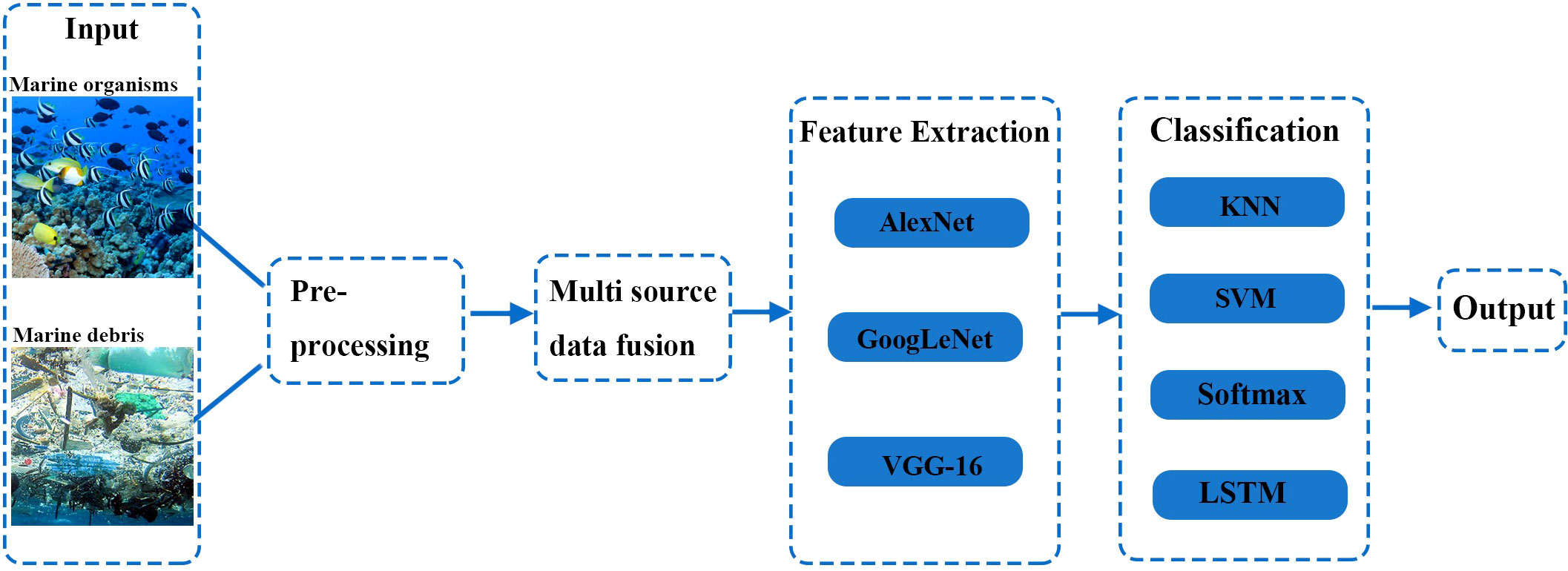
Figure 1 The general framework of the proposed methodology.

3.2 Data collection

In this research, we use two different databases for each indicators that are publicly available for simulations and experimental work, as depicted in Table 1. These two databases for each indicators are fused together to evaluate the model. A few images of the underwater objects are depicted in Figure 2. Table 2 shows the class-wise distribution of the samples used in our experiments. In our experiments, there are two major datasets. One is for marine debris images, and the other is for marine organism images. Each dataset is divided into six distinct categories, with each category being represented by synapomorphies. The dataset is divided into three subsets: 60% of the data to the training set, 20% to the validation set, and 20%to the test set. In this study, a ten-fold cross-validation approach is used. Moreover, considering the complexity of the problem and the size of the dataset, the balance between positive and negative samples in the training dataset, the validation dataset, and the test dataset is crucial to avoid biased learning and ensure the model’s ability to generalize well, as shown in Table 3.

TABLE 1

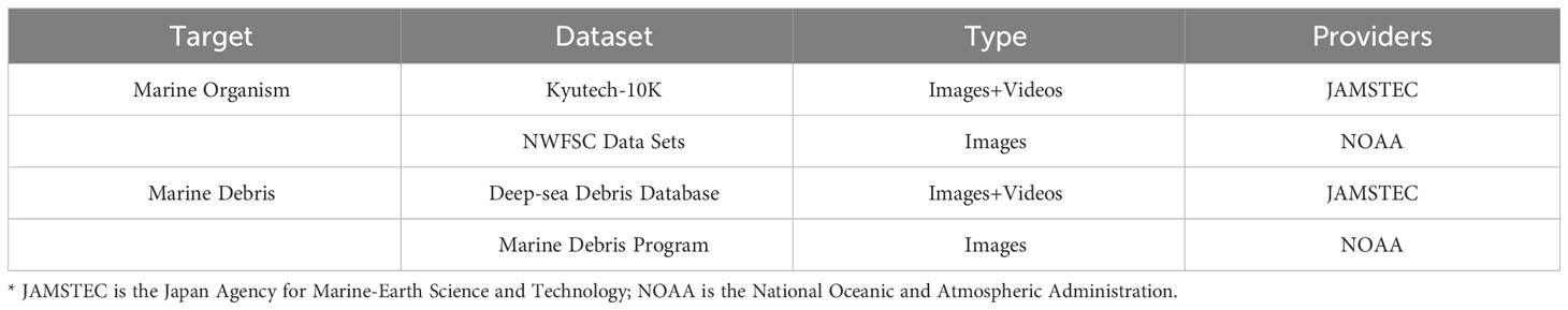
Table 1 Datasets for marine organisms and marine debris.

FIGURE 2

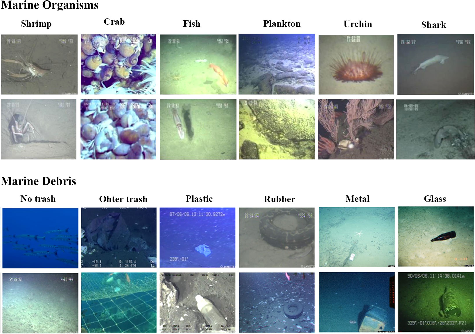
Figure 2 Sample of images from the datasets.

TABLE 2

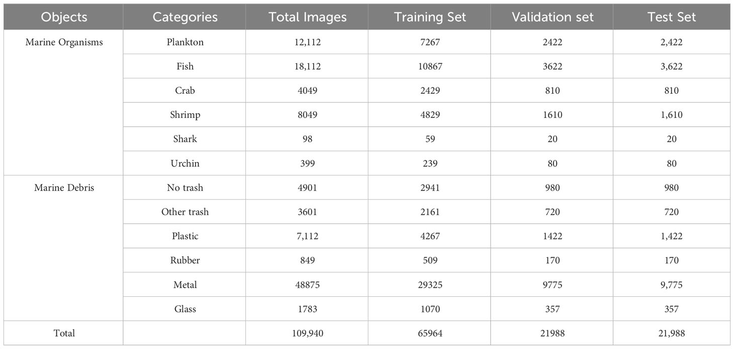
Table 2 Distribution of categories in the dataset.

TABLE 3

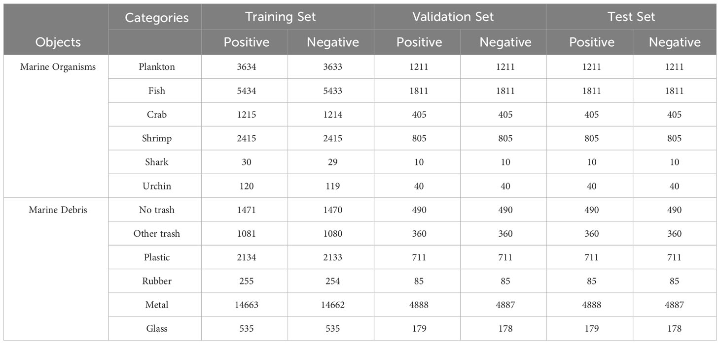
Table 3 The numbers of positive and negative of training dataset, validation dataset, and test dataset among twelve categories.

3.3 Preprocessing of data

In this research, data preprocessing included two parts: image-size standardization and data augmentation. In order to mitigate the impact of different properties and numerical differences in the data, the raw data were standardized. By standardizing the image size, We can input the images to the model without additional resizing, regardless of their original dimensions. Also, standardizing the image size can help reduce computational complexity and memory usage during training as well as improve the overall performance and accuracy of the model.

Data augmentation aims to increase the number of training samples and enhance the dimension and diversity of the data. After conducting image-size standardization, data augmentation was employed to artificially increase the size of the dataset and effectively prevent overfitting. In this study, we employ four distinct types of image set augmentation, such as flip, crop, translation, and affine transformation. These methods enable transformed images to be created with the same label as the original images. Firstly, we vertically flip all images to recognize underwater and surface objects regardless of their orientation. Next, we crop the images by removing about one-fifth of the right and left edges. Thirdly, we randomly shift images by certain amounts of pixels, which could assist in recognizing the object or segment regardless of its position in the image. Lastly, we apply an affine transformation based on sine transforms to each training image, generating multiple images of each object from different view angles.

3.4 Multi-source data fusion

Multi-source data fusion refers to the process of integrating and combining information from multiple diverse sources to derive comprehensive insights and make informed decisions. By harnessing the power of various data streams, multi-source data fusion enables a more holistic understanding of complex phenomena. This fusion process involves data preprocessing, feature extraction, and integration techniques, which aim to improve the quality of the data and enhance the accuracy of the analysis. In this study, the image datasets of marine organisms and debris were selected. Once the data is collected, it needs to be preprocessed to ensure consistency and quality. Data preprocessing aims to make the data suitable for further analysis and fusion. Next, their dimensional data was fused using data fusion algorithms. As the input values varied, they were multiplied by distinct weights to account for these differences. The resulting input map can be obtained by combining the data as illustrated:

$\begin{array}{ll}{X}_{\text{output}}=(W_{\text{turb}}\times X_{\text{turb}})+W_{\text{pose}}+X_{\text{pose}})+W_{\text{variety}}\times X_{\text{variety}}& (1)\end{array}$

where X is applied for element wise multiplication and X_turb, X_pose, X_variety represent the input, W_turb, W_pose, W_variety depict the learning parameters classifying numerous impact degree of these factors.

To normalize the output values, a hyperbolic function presents in Equation 2. It is utilized to define a particular range (−1, 1). The value at the t time interval is represented by $\widehat{X_t}$.

$\begin{array}{ll}{\widehat{X}}_t=\tanh (X_{\text{output}})& (2)\end{array}$

3.5 Feature extraction

Deep CNNs are a type of neural network that is specifically designed for processing images and other spatial data. They consist of multiple layers of convolutional and pooling operations, followed by fully connected layers for classification or regression tasks. Currently, deep CNNs are widely used in various computer vision applications for object detection, image segmentation, and image classification. Features extracted by deep CNNs always achieve better performance than other methods. AlexNet, GoogLeNet, and VGG-16, which are the most frequently used in previous research, are selected and used in this study.

3.5.1 AlexNet

AlexNet is one of the well-known deep CNN architectures, which was developed by Alex Krizhevsky, Ilya Sutskever, and Geoffrey Hinton in 2012. AlexNet won the championship in the ImageNet Large Scale Visual Recognition Challenge 2012 (ILSVRC) competition, achieving a top-5 error rate of 15.3%. The architecture of AlexNet is composed of eight layers, which are five convolutional layers and three fully-connected layers (see Figure 3). The network, except the last layer, is divided into two copies, which are processed on the GPU (Krizhevsky et al., 2017). More specifically, In the first layer, the size of a convolutional layer of 11 × 3 and a stride of 4 pixels are used. The second convolutional layer filter size was reduced to 5 × 5 × 48, and the convolutional stride was reduced to 1. The third convolutional layer consists of 384 kernels with a size of 3 × 3 × 256 applied with a stride of 1. The fourth and fifth convolutional layers have 384 kernels with a size of 3 × 3 × 192 and 256 kernels with a size of 3 × 3 × 128 respectively. These layers also have a stride of 1. The two first and last convolutional layers are followed by max-pooling layers, where the size of the pooling layer is 3 × 3 and a stride of 2. Hence, the output size is reduced by half in each of these pooling layers. Following the three fully connected layers, AlexNet outputs 1000 classes in the ImageNet dataset. AlexNet achieves remarkable performance due to data augmentation, dropout, ReLU, standardization, and overlapping pooling.

FIGURE 3

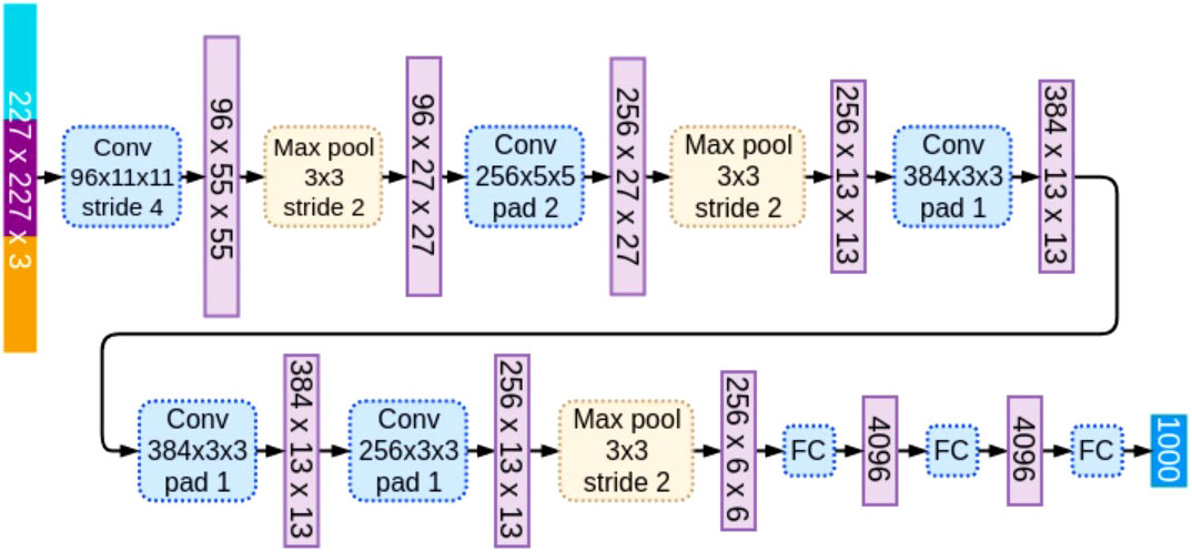
Figure 3 AlexNet architecture.

3.5.2 GoogLeNet

GoogLeNet is a 22-layer deep convolutional neural network that was proposed by Szegedy et al. (2015) at Google in 2014 (see Figure 4). It was designed to reduce the number of parameters in the model, thereby reducing computational complexity and improving the accuracy and efficiency of image classification tasks. Hence, the GoogLeNet achieved state-of-the-art performance in classification and detection, used fewer parameters, and ran faster than previous models, with a top-5 test error rate of 6.7% in the ILSVRC-2014 competition. GoogLeNet employs a unique type of network block called an inception module, which consists of multiple parallel convolutional and pooling layers, as shown in Figure 2. The Inception module consists of parallel convolutional layers with different filter sizes, including 1 × 1, 3 × 3, and 5 × 5 filters, as well as pooling operations. These parallel paths capture information at various spatial scales and enable the network to learn both local and global features. Additionally, 1 × 1 convolutions are used to reduce the dimensionality of the input data and control computational complexity. GoogLeNet employs a 1 × 1 convolutional layer as a bottleneck layer to minimize input channels. Then the convolutional layer put into multiple parallel convolutional and pooling layers of different sizes, which could solve the alignment issues. To combat the issue of vanishing gradients in deep networks, GoogLeNet introduced auxiliary classifiers at intermediate layers. These auxiliary classifiers provide additional supervision during training and help propagate gradients back to earlier layers, aiding in the training of deeper networks.

FIGURE 4

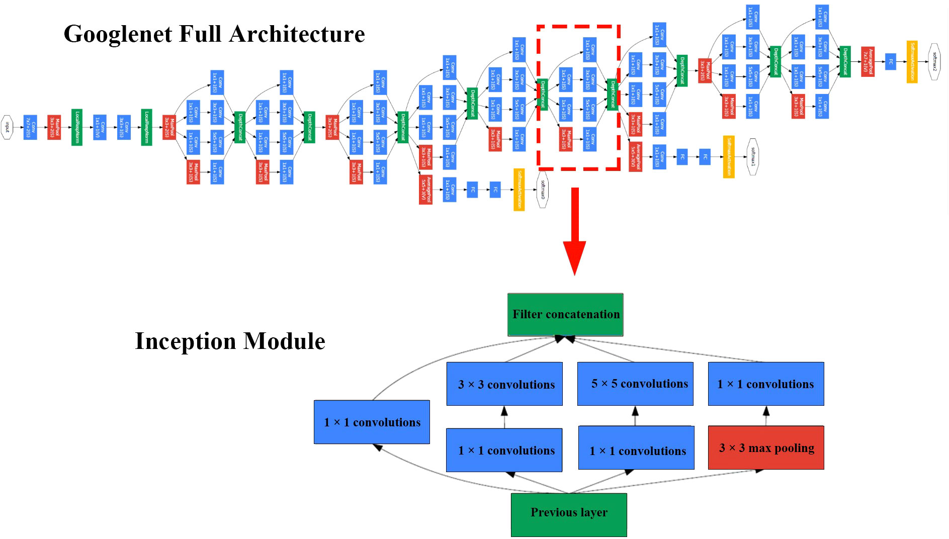
Figure 4 GoogLeNet architecture.

3.5.3 VGG-16

VGG-16 is a kind of deep CNN model that was developed by Alberto et al. from the Visual Geometry Group at the University of Oxford in 2014 (Garcia-Garcia et al., 2017). The VGG-16 method achieved state-of-the-art performance on ILSVRC 2014, achieving 92.7% top-5 test accuracy on the ImageNet dataset. The architecture of VGG-16 consists of 16 layers, which are 13 convolutional layers and 3 fully connected layers. VGG-16 receives an image input size of 224 × 224. Then it is processed by a series of convolutional layers with 3 × 3 filters, followed by max-pooling layers with 2 × 2 filters with stride 2. After a stack of convolutional layers, there are two fully-connected layers with 4096 channels each and one output layer with 1000 channels. The structure of VGG-16 is described by the following Figure 5.

FIGURE 5

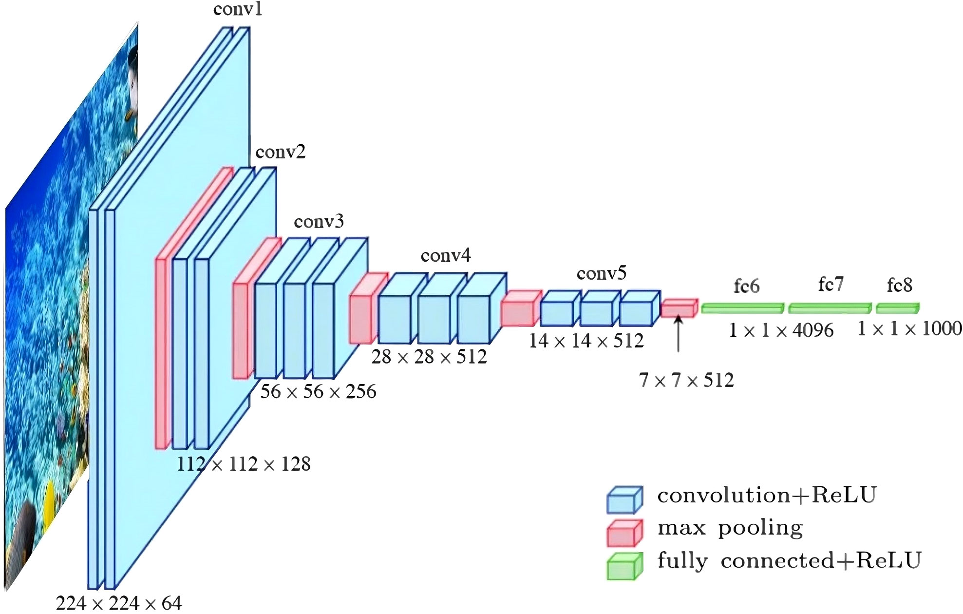
Figure 5 VGG-16 architecture.

3.6 Deep feature classification with conventional machine and deep learning classifiers

The most common classifiers have gained excellent results, which are KNN, SVM, softmax, and LSTM. These four classifiers were trained on deep features extracted with the best performing feature extraction scheme.

3.6.1 KNN

KNN is a simple and effective algorithm for classification in machine learning. Generally, KNN has better performance than neural networks on a training dataset. The performance of the KNN classifier is mainly influenced by the key parameter k. When introducing the KNN classifier, setting a higher K value can produce a smoother decision boundary that could reduce the impact of noisy data and lead to overgeneralization. Conversely, a lower K value may lead to a more complex decision boundary that may cause overfitting. Euclidean distance is the most commonly used distance function when dealing with fixed-length vectors of real numbers. the equation is

$\begin{array}{ll}d(x,y)=\left|\right|x-y\left|\right|=\sqrt{(x-y}·(x-y)={\left({\displaystyle \sum _{i=1}^m(x_i-y_i}{)}^2\right)}^{1/2}& (3)\end{array}$

KNN is a widely employed supervised learning technique utilized in various domains, such as data mining, statistical pattern recognition. KNN operates by classifying objects based on their proximity to the nearest training examples in the feature vector. The classification of an object is determined by a majority vote of its closest neighbors, with K being a positive integer that signifies the number of neighbors considered. These neighbors are selected from a set of known correct classifications. While the Euclidean distance is commonly used, alternative distance measures like the Manhattan distance can also be employed.

3.6.2 SVM

SVM uses a linear model to implement nonlinear boundaries between classes by mapping the original data from the input space to a high-dimensional feature space. This mapping constructs a new space by using a set of kernel functions. After this mapping, an optimal separating hyperplane is achieved by maximizing the margins of class boundaries with respect to the training data (Tajiri et al., 2010). For the case of linearly separable data, a separating hyperplane about the binary decision classes can be represented as the following equation:

$\begin{array}{ll}{y}_i[w{x}_i+b]\ge 1,{\forall }_i& (4)\end{array}$

where x_i and b represent the attribute values and bias, respectively, and wis a coefficient vector that determines the hyperplane in the feature space. This formula constructs two hyperplanes that find the optimal hyperplane with a maximal margin by minimizing ∥w∥², subject to constraints. The above formulation could cause a particular dual problem called the Wolfe dual (Fletcher and Shawe-Taylor, 2013). Therefore, the formula will be formed as follow:

$\begin{array}{ll}{L}_D\equiv {\displaystyle \sum _{i=1}^N{\alpha }_i}-\frac{1}{2}{\displaystyle \sum _{i=1}^N{\displaystyle \sum _{j=1}^N{\alpha }_i{\alpha }_j{y}_i{y}_{j}K(x_i,x_j)}}& (5)\end{array}$

Subject to

$\begin{array}{ll}0\le {\alpha }_i\le C,{\forall }_i& (6)\end{array}$

$\begin{array}{ll}{\displaystyle \sum _{i=1}^N{\alpha }_i{y}_i=0}& (7)\end{array}$

where k(x_i,x_j) is a kernel function representing the inner product between x_i and x_j in the feature space. Four types of kernel functions are often used to solve different problems which are the linear kernel, the polynomial kernel, the radial basis kernel (RBF), and the sigmoid kernel. The choice of kernel function is based on the problem type. The final SVM classifier will be in the form of:

$\begin{array}{ll}f(x)=sign\left({\displaystyle \sum _{i=1}^N{a}_i{y}_{i}K(x,x_i)+b}\right)& (8)\end{array}$

3.6.3 Softmax

The softmax classifier is a widely used method for multi-class classification in machine learning and deep learning that achieves excellent performance for multi-class tasks. In the context of deep learning, the softmax classifier is a neural network architecture that employs the softmax function as the final layer for classification tasks. The softmax function takes an input vector and normalizes it into a probability distribution whose total sums up to 1. The softmax function can be used in a classifier only when the classes are mutually exclusive. The softmax function formula is as follows:

$\begin{array}{ll}\sigma {(\overrightarrow{z})}_i=\frac{e^{zi}}{{\displaystyle {\sum }_{j=1}^K{e}^{z_j}}}& (9)\end{array}$

where all z_i values are the elements of the input vector and can take any real value. The term at the bottom of the formula is the normalization term, which ensures that all the output values of the function will sum to 1, thus constituting a valid probability distribution.

3.6.4 LSTM

LSTM is a variant of Recurrent Neural Network (RNN), which is designed to solve the vanishing gradient problem of RNN. A memory cell in the LSTM model is an important reason for addressing the problem of RNN. The memory cell is controlled by three gates, which are a forget gate f_t, an input gate i_t, and an output gate o_t. These three gates assist in regulating the information flow through the memory cell. In LSTM, the forget gate plays an important role in deciding what information should be forgotten or remembered from its memory. It controls the information flow through cell state, and its calculation is shown in Equation:

$\begin{array}{ll}ft=\sigma W_i[h_{t-1,}{x}_t]+b_f)& (10)\end{array}$

Here, σ denotes the sigmoid function, which maps the input values to the interval (0, 1). h_t−1 is the previous hidden state. x_t is the current node. W_f represents the weight parameters. b_f represents the bias parameters. The weight and bias parameters are learned during the LSTM training process.

The Input gate is employed to fresh data into the memory cell through element-wise multiplication with the new input. The input gate consists of the input activation gate and the candidate memory cell gate, which allow the LSTM to update and govern the data in the memory. The input gate is calculated by the equation in the LSTM network, which determines values of the cell state should be modified based on an input signal. This modification is carried out using a sigmoid function and a Hyperbolic tangent (tanh) layer, as shown in Equation (11), and results in the creation of a candidate memory cell vector Eqation (12).

$\begin{array}{ll}{i}_t=\sigma W_i[h_{t-1},x_t]+b_f)& (11)\end{array}$

$\begin{array}{ll}\tanh =\left(\frac{e^x-e^{-x}}{e^x+e^{-x}}\right)& (12)\end{array}$

$\begin{array}{ll}{\tilde{c}}_t=\text{ tanh}(W_c[{ht-}_1,x_t]+b_c)& (13)\end{array}$

To update the previous memory cell c_t−1, the input vector and the candidate memory cell vector are combined, which is represented as:

$\begin{array}{ll}{c}_t=f_t\odot c_t-1+i_t\odot {\tilde{c}}_t& (14)\end{array}$

where ⊙ denotes element-wise multiplication.

The output gate is used to combine with the current memory cell to produce the current hidden state, and the current hidden state influences the output at the next time step. The calculation process is shown as:

$\begin{array}{ll}{o}_t=\sigma (W_o[{ht-}_1,x_t,c_t]+b_o)& (15)\end{array}$

The structure of LSTM is shown in Figure 3. The LSTM method addresses the problem of long-term dependence in learning, which provides good forecasting results.

3.7 Model performance evaluation

In examining the performance of monitoring marine pollution, we adopted the accuracy, precision, sensitivity, and F1-score based on their suitability for the performance measures of different classifiers in this study. The four estimators are described and calculated as follows:

$\begin{array}{ll}Accuracy=\frac{TP+TN}{TP+TN+FP+FN}& (16)\end{array}$

$\begin{array}{ll}Precision=\frac{TP}{TP+FP}& (17)\end{array}$

$\begin{array}{ll}Sensitivity=\frac{TP}{TP+FN}& (18)\end{array}$

$\begin{array}{ll}F1=\frac{2TP}{2TP+FN+FP}& (19)\end{array}$

where TP presents True Positive, FN refers to False Negative, TN is True Negative and FP is False Positive.

4 Experimental results

All the experiments, including data processing, feature extraction, and data classification are carried out on MATLAB 2018a and Python3.6 programming implementation.

4.1 Features extracted by different deep CNN architectures

According to our proposed framework, deep CNN models are utilized to extract image features. Figure 6 illustrates the training and validation losses for all employed deep CNN models trained under the same training dataset. The validation loss curves closely follow the corresponding training loss curves, showing the ability of the deep CNN models in generalization.

FIGURE 6

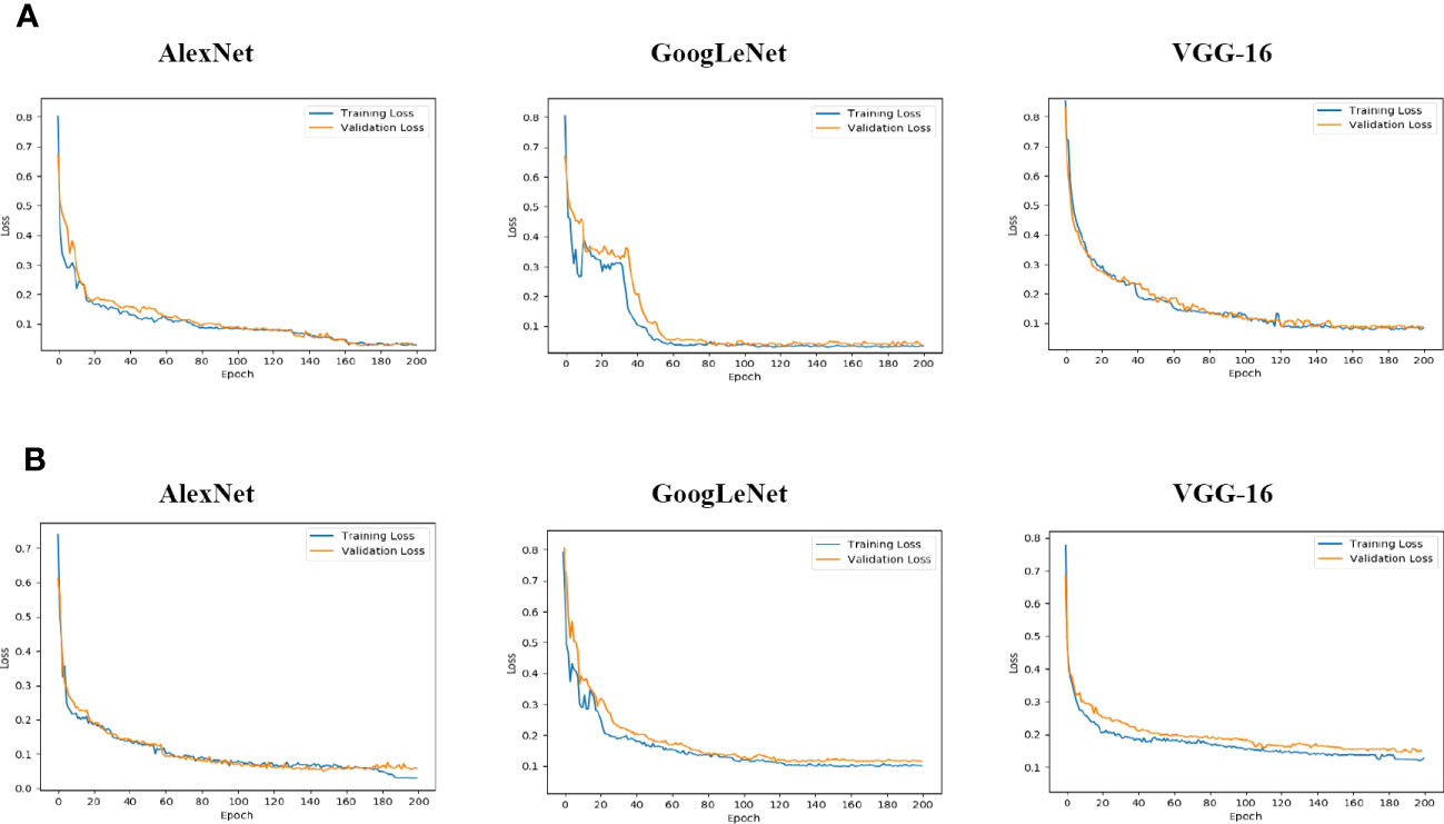
Figure 6 Average loss per epoch for training and validation steps. (A) Loss of the training and validation with respect to epoch of marine organism detection. (B) Loss of the training and validation with respect to epoch of marine debris detection.

We compare the performance of AlexNet, GoogLeNet, and VGG-16 for marine organism and debris detection. We can see that VGG-16 achieves the best performance of marine organisms in Table 4, which obtained the best results of all considered metrics, including 93.39% accuracy, 95.34% precision, 90.74% sensitivity, and 93.54%F1-score. Table 4 and Figure 7 show four estimators for each deep CNN architecture for different categories of marine organism detection. The VGG-16 extractor for plankton detection shows the best performance with 98.57% accuracy, 97.76% precision, and 96.92% F1-score. The AlexNet extractor for plankton detection achieves a highest sensitivity of 93.76%. In contrast, The GoogLeNet extractor shows the weakest performance in crab detection with 82.05% accuracy and 86.45% precision. The AlexNet extractor for shrimp recognition obtains the lowest sensitivity of 78.06% and the lowest F1-score of 79.89%.

FIGURE 7

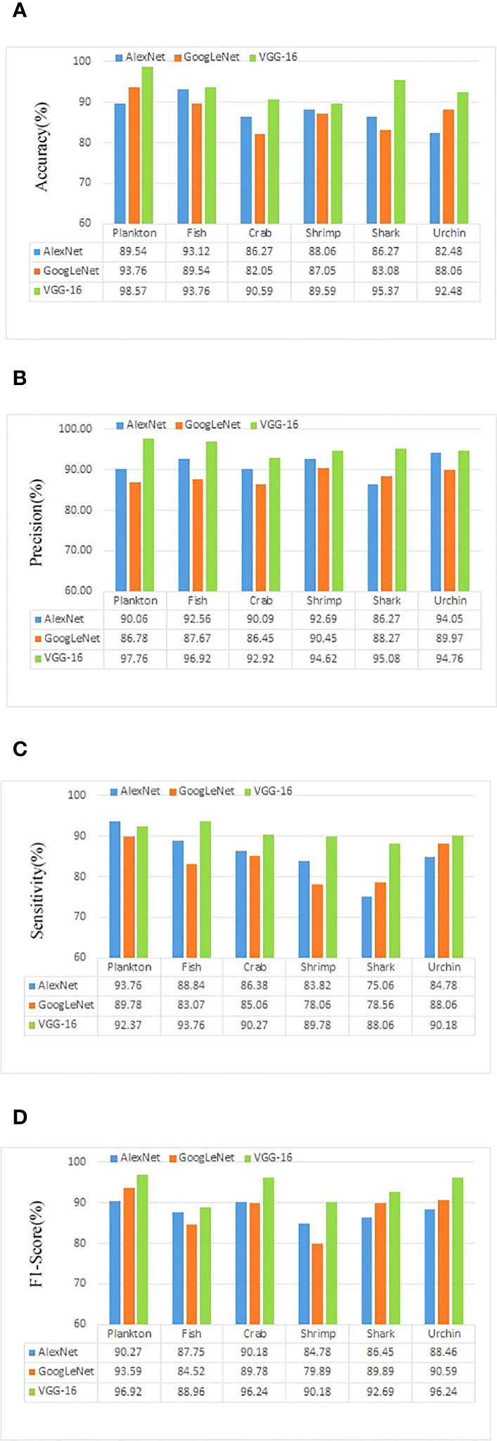
Figure 7 The performance of four estimators of marine organism detection. (A) The Accuracy of deep CNNs. (B) The Precision of deep CNNs. (C) The Sensitivity of deep CNNs. (D) The F1-score of deep CNNs.

TABLE 4

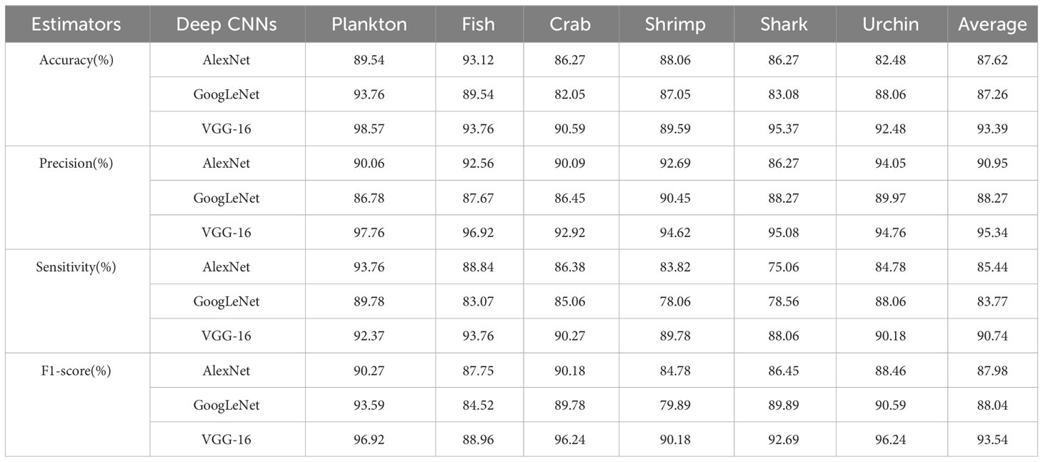
Table 4 Results of performance with different deep CNNs of marine organism detection.

In terms of marine debris detection, AlexNet achieves the best result with 92.41% accuracy, 92.04% precision, 93.08% sensitivity, and 91.95% F1-score, as shown in Table 5. Figure 8 shows four estimators for each deep CNN architecture for different categories of marine debris detection. The best performance is observed on rubber detection using the AlexNet extractor, which achieves a highest accuracy of 95.37%, a highest precision of 96.27%, a highest sensitivity of 96.59%, and a highest F1-score of 96.24%. In contrast, the weakest performance is observed on other trash detection using the GoogLeNet extractor, with a lowest accuracy of 78.06%, a lowest precision of 83.05%, and a lowest sensitivity of 82.48%. The VGG-16 extractor shows the worst performance in no trash recognition with the lowest F1-score of 78.45%.

TABLE 5

Table 5 Results of performance with different deep CNNs of marine debris detection.

FIGURE 8

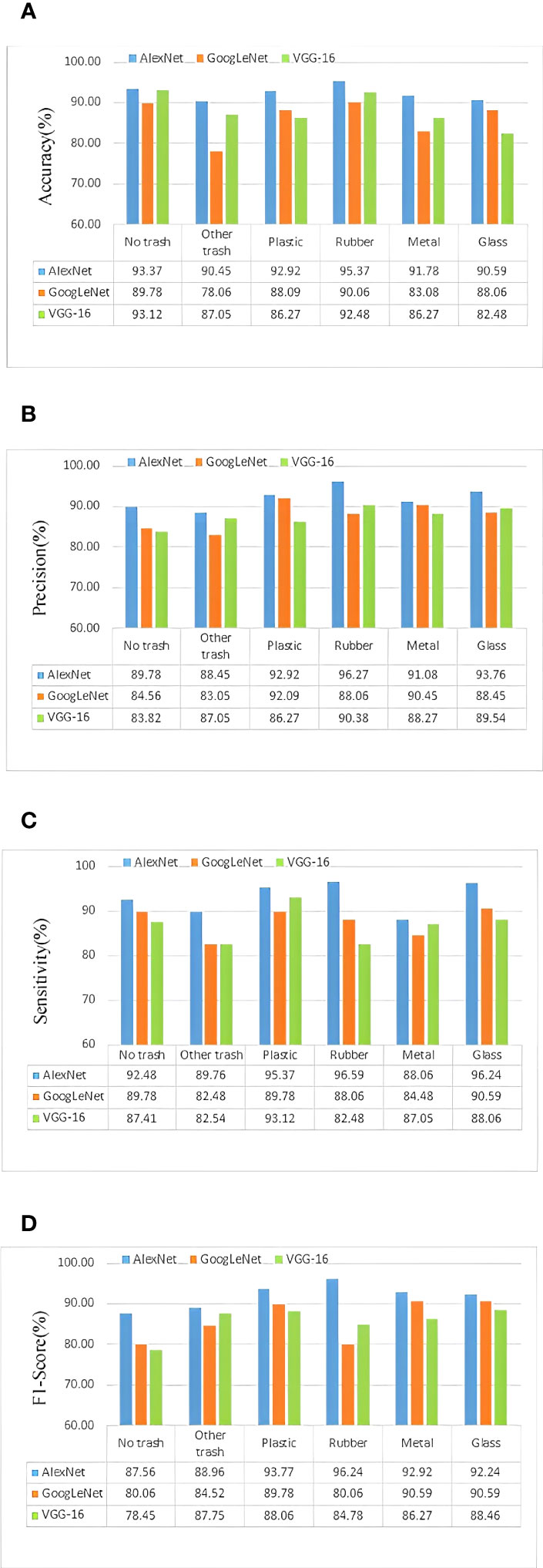
Figure 8 The performance of four estimators of marine debris detection. (A) The Accuracy of deep CNNs. (B) The Precision of deep CNNs. (C) The Sensitivity of deep CNNs. (D) The F1-score of deep CNNs.

In this study, the receiver operating characteristics (ROC) curve and the area under curve (AUC) is employed in these two scenarios to determine the validity of the proposed method. The ROC curve is a way of displaying the true positive rate (TPR) against the false positive rate (FPR) at different thresholds, which reflect sensitivity and 1-specicity value of the proposed method. Figure 9 shows the ROC curve of all subjects and the average AUC of all subjects in marine organism and debris detection. In marine organism detection, ROC analysis showed that the average AUC of the VGG-16 method is 0.80 and is significant (p¡0.05), which outperform than other deep CNNs. In terms of marine debris recognition, the average AUC of AlexNet is around 0.88 and is significant (p¡0.05). According to the results, it shows that the AlexNet method had the best performance among three deep CNNs.

FIGURE 9

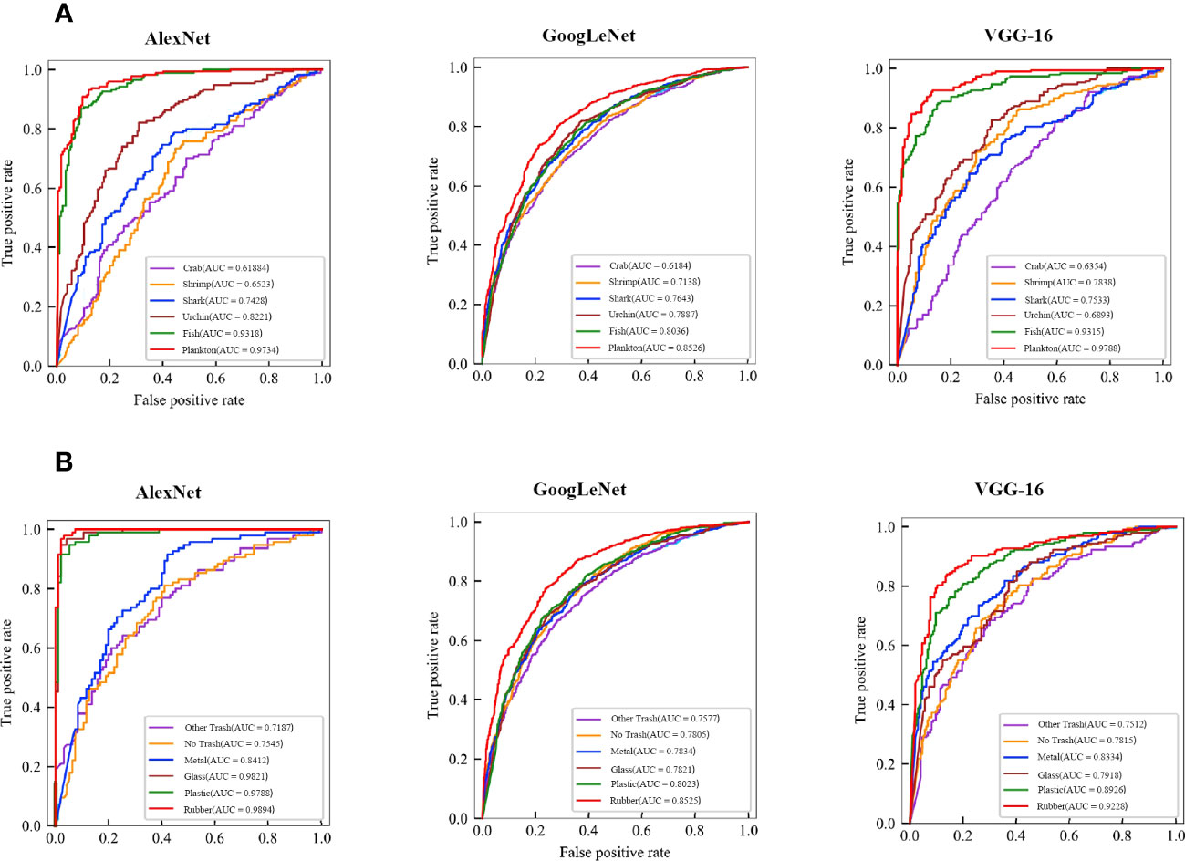
Figure 9 The ROC curves and AUC values of three different deep CNNs. (A) Marine organism detection. (B) Marine debris detection.

In this study, t-SNE is used to visually compare differences among these three deep CNN architectures in marine organism and debris detection. Figure 10 shows two-dimensional t-SNE training feature projections for the best-performing VGG-16 architecture for marine organism detection and AlexNet architecture for marine debris detection when three different schemes of transfer learning are used.

FIGURE 10

Figure 10 Two-dimensional t-SNE projections of three deep CNNs. (A) t-SNE of marine organism detection. (B) t-SNE of marine debris detection.

4.2 Performance of machine and deep learning classifiers

In this study, KNN, SVM, Softmax, and LSTM classifiers are trained on deep features extracted with the best-performing feature extraction methods for a given CNN architecture. As we can see from Table 6, the LSTM classifier with VGG-16 for detecting marine organisms outperforms other deep learning models with 95.99%, 95.21%, 97.48%, and 98.24% for accuracy, precision, sensitivity, and F1-score, respectively. As shown in Table 7, the best performance was observed with the AlexNet extractor, which obtained the best classification result with an LSTM with an accuracy of 98.68%, precision of 96.76%, sensitivity of 95.42%, and F1-score of 96.24%.

TABLE 6

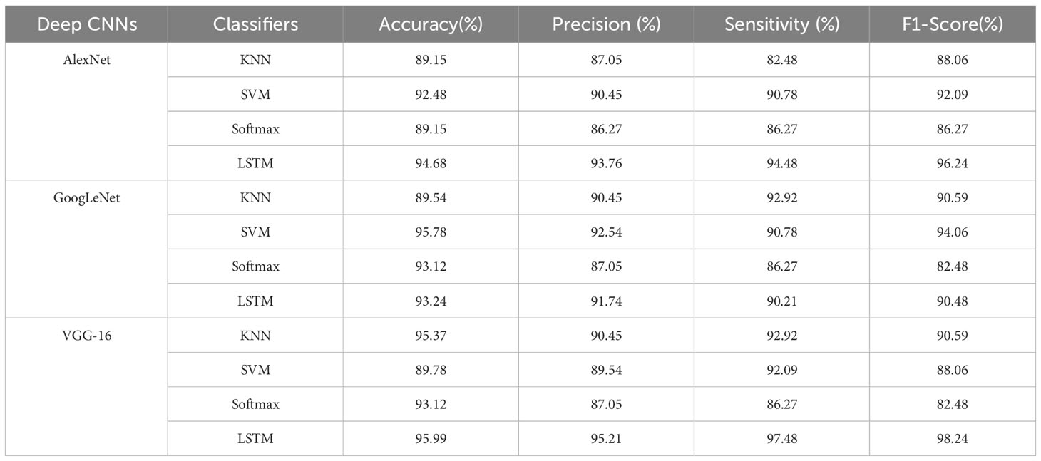
Table 6 Results of performance of AI methods on deep feature extractor of marine organism detection.

TABLE 7

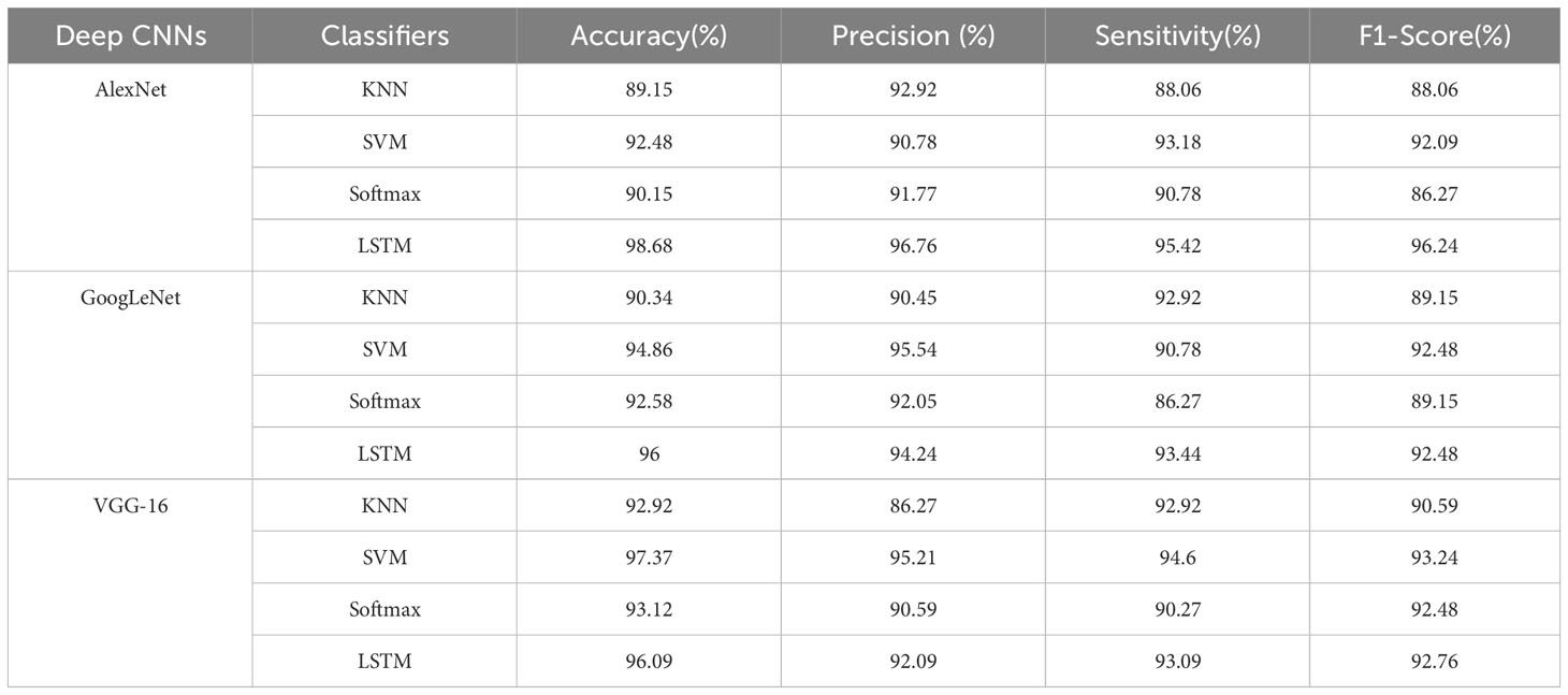
Table 7 Results of performance of AI methods on deep feature extractor of marine debris detection.

Figure 11 shows the accuracy on the test set when each algorithm performs ten-fold cross validation on the marine organism dataset. It can be seen in the figure that the classification effect of VGG-16-LSTM algorithm with green line is the best in all ten-fold test sets. In terms of the marine debris dataset, the classification effect of AlexNet-LSTM algorithm with yellow line is the best in all ten-fold test sets and the result fluctuation is small.

FIGURE 11

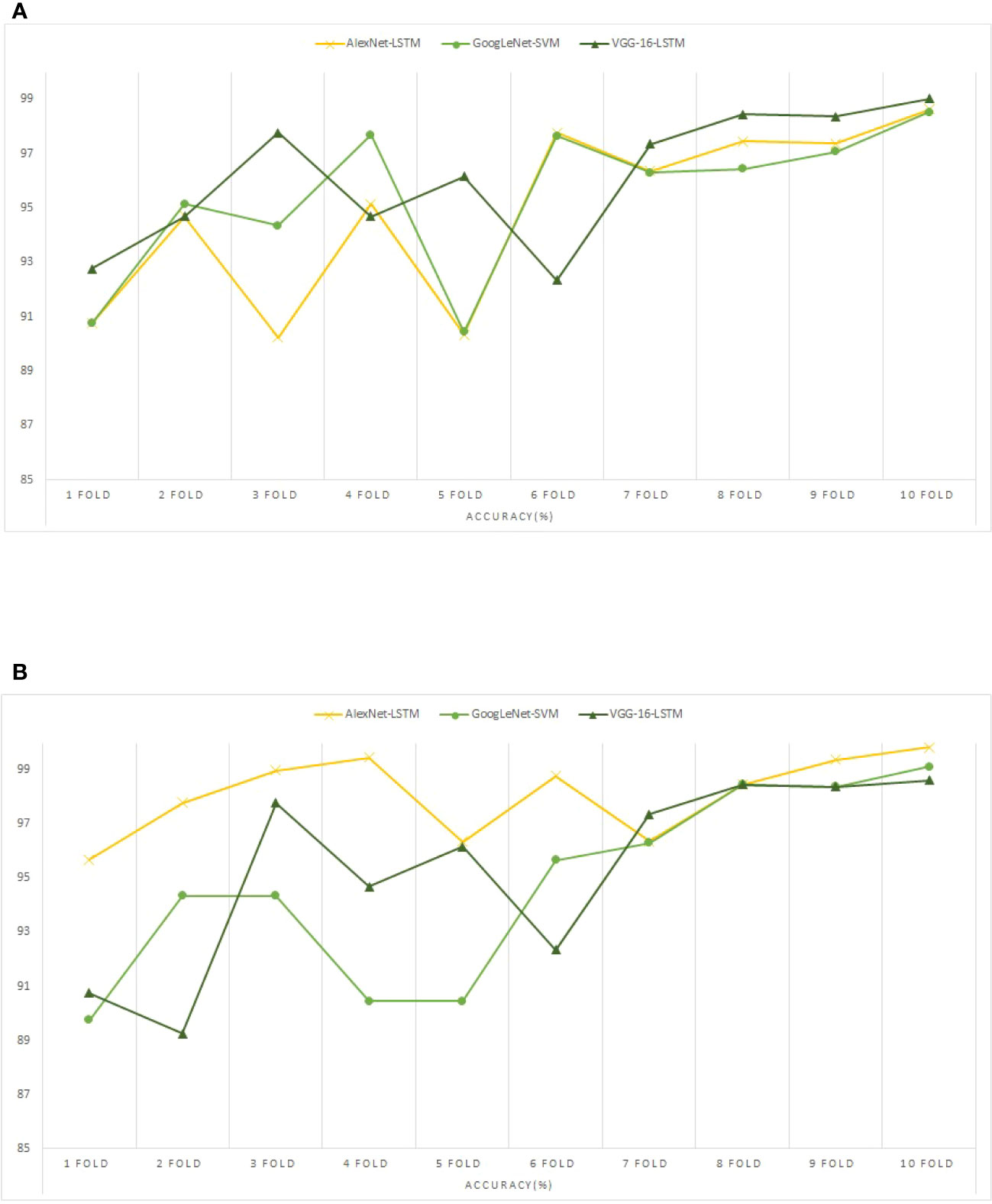
Figure 11 Ten-fold test set classification accuracy. (A) Marine organism detection. (B) Marine debris detection.

Normalized confusion matrices in Figure 12 display the performance of deep CNNs with machine and deep learning classifiers on marine organism and debris detection. The confusion matrices for the best-performing VGG-16-LSTM for marine organism detection and AlexNet-LSTM for marine debris detection.

FIGURE 12

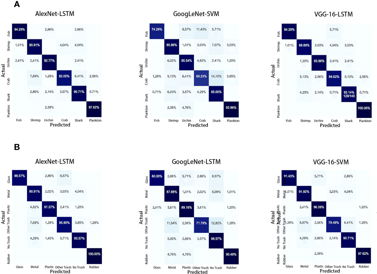
Figure 12 Confusion matrices. (A) Confusion matrices of marine organism detection. (B) Confusion matrices of marine debris detection.

5 Discussion and conclusions

Marine pollution is a major environmental challenge that affects the health of the world’s oceans and the creatures that live in them, thereby negatively impacting carbon neutrality. The sources of marine pollution are diverse, including land-based sources such as industrial and municipal waste, agricultural runoff, and litter, as well as ocean-based sources such as oil spills and ship discharges. Due to the complexity of monitoring marine pollution, most previous research used a single ocean indicator to monitor marine pollution. In this paper, we used marine organisms and marine debris as two ocean indicators for monitoring marine pollution. Motivated by the need for automatic and effective approaches for marine organism and debris monitoring, we employ machine and deep learning techniques together with deep learning-based feature extraction to identify and classify marine organisms and debris in a realistic underwater environment.

This paper provides a comparative analysis of common deep conventional architectures used as feature extractors for underwater image classification. Furthermore, it explores the best ways to use deep feature extractors by analyzing three different modes for utilizing pretrained deep feature extractors and examining the performance of different machine and deep learning classifiers trained on top of extracted features. Our results show that VGG-16 achieves the best performance of marine organism detection, which obtained the best results of all considered metrics, including 95.99% accuracy, 95.21% precision, 97.48% sensitivity, and 98.24%F1-score.However, the AlexNet extractor for marine debris detection shows the best performance with 92.41% accuracy, 92.04% precision,93.08% sensitivity, and 91.95% F1-score. Our results also show that four common classifiers are used to train on features extracted with deep CNNs. The LSTM trained on the VGG-16 extractor achieves the best performance with 95.99% accuracy, 95.21% precision, 97.48% sensitivity, and 98.24% F1-score for detecting marine organisms, while the LSTM classifier trained on the AlexNet extractor obtains accuracy of accuracy of 98.68%, precision of 96.76%, sensitivity of 95.42%, and F1-score of 96.24%. Considering the inherent challenges that come with automatic marine organism and debris classification in underwater imagery, the obtained results demonstrate the potential for further exploitation of deep-learning-based models for marine organism and debris identification and classification in complex marine environments.

However, three major limitations of our study should be mentioned. First, this study only selected six categories for each dataset. It is relatively limited. Future studies should consider expanding the range of categories for marine organism and debris recognition and classification. Including a broader spectrum of categories would allow for a more comprehensive understanding of the marine ecosystem and pollution dynamics. This expansion can be achieved by collecting more diverse datasets and incorporating advanced classification techniques. Second, most underwater videos have limited discriminative information due to their low resolution and low saturation. Enhancing the quality of data collection is crucial for improving the accuracy and reliability of classification models. Future studies may explore the use of higher-resolution underwater cameras and advanced imaging technologies to capture more detailed and informative data. Additionally, considering variations in lighting conditions, water clarity, and camera positioning can further improve the quality and representativeness of the collected data. Third, it is the first time to detect two ocean indicators for marine pollution. It might cause uncertainty, which impacts the experiment due to a lack of experience. In the future, we could incorporate multi-modal data, such as acoustic or hydrodynamic information, which can provide a richer context for marine organism and debris recognition. Combining visual data with other sensor modalities can enhance the accuracy of classification models and provide a more comprehensive understanding of marine ecosystems and pollution dynamics. Future research can explore the fusion of different data sources to improve classification performance.

Data availability statement

The original contributions presented in the study are included in the article/supplementary material. Further inquiries can be directed to the corresponding author.

Author contributions

BW: Conceptualization, Formal Analysis, Methodology, Software, Validation, Visualization, Writing – original draft, Writing – review & editing. LH: Conceptualization, Formal Analysis, Methodology, Software, Supervision, Validation, Writing – original draft, Writing – review & editing. HM: Data curation, Resources, Validation, Writing – original draft, Writing – review & editing. YK: Data curation, Resources, Software, Validation, Writing – review & editing. NZ: Data curation, Resources, Software, Validation, Writing – review & editing.

Funding

The author(s) declare financial support was received for the research, authorship, and/or publication of this article. This work was sponsored in part by Science and Technology Development Fund 2021KJ018.

Acknowledgments

The authors thank the participants for their valuable time in data collecting.

Conflict of interest

The authors declare that the research was conducted in the absence of any commercial or financial relationships that could be construed as a potential conflict of interest.

Publisher’s note

All claims expressed in this article are solely those of the authors and do not necessarily represent those of their affiliated organizations, or those of the publisher, the editors and the reviewers. Any product that may be evaluated in this article, or claim that may be made by its manufacturer, is not guaranteed or endorsed by the publisher.

References

Ahn J., Yasukawa S., Sonoda T., Nishida Y., Ishii K., Ura T. (2018). An optical image transmission system for deep sea creature sampling missions using autonomous underwater vehicle. IEEE J. Oceanic Eng. 45, 350–361. doi: 10.1109/JOE.2018.2872500

CrossRef Full Text | Google Scholar

Bazi Y., Bashmal L., Rahhal M. M. A., Dayil R. A., Ajlan N. A. (2021). Vision transformers for remote sensing image classification. Remote Sens. 13, 516. doi: 10.3390/rs13030516

CrossRef Full Text | Google Scholar

Chin C. S., Neo A. B. H., See S. (2022). “Visual marine debris detection using yolov5s for autonomous underwater vehicle,” in IEEE/ACIS 22nd International Conference on Computer and Information Science (ICIS). (Zhuhai, China: IEEE), 20–24. doi: 10.1109/ICIS54925.2022.9882484

Google Scholar

Chuang M.-C., Hwang J.-N., Williams K., Towler R. (2011). “Automatic fish segmentation via double local thresholding for trawl-based underwater camera systems,” in 2011 18th IEEE International Conference on Image Processing. Brussels, Belgium: IEEE, 3145–3148. doi: 10.1109/ICIP.2011.6116334

CrossRef Full Text | Google Scholar

Duan G., Nur F., Alizadeh M., Chen L., Marufuzzaman M., Ma J. (2020). Vessel routing and optimization for marine debris collection with consideration of carbon cap. J. Clean. Prod. 263, 121399. doi: 10.1016/j.jclepro.2020.121399

CrossRef Full Text | Google Scholar

El Zrelli R., Rabaoui L., Alaya M. B., Daghbouj N., Castet S., Besson P., et al. (2018). Seawater quality assessment and identification of pollution sources along the central coastal area of gabes gulf (se Tunisia): evidence of industrial impact and implications for marine environment protection. Mar. pollut. Bull. 127, 445–452. doi: 10.1016/j.marpolbul.2017.12.012

PubMed Abstract | CrossRef Full Text | Google Scholar

Fletcher T., Shawe-Taylor J. (2013). Multiple kernel learning with fisher kernels for high frequency currency prediction. Comput. Economics 42, 217–240. doi: 10.1007/s10614-012-9317-z

CrossRef Full Text | Google Scholar

Franklin J. B., Sathish T., Vinithkumar N. V., Kirubagaran R. (2020). A novel approach to predict chlorophyll-a in coastal-marine ecosystems using multiple linear regression and principal component scores. Mar. pollut. Bull. 152, 110902. doi: 10.1016/j.marpolbul.2020.110902

PubMed Abstract | CrossRef Full Text | Google Scholar

Fulton M., Hong J., Islam M. J., Sattar J. (2019). “Robotic detection of marine litter using deep visual detection models,” in 2019 international conference on robotics and automation (ICRA). Montreal, QC, Canada: IEEE, 5752–5758. doi: 10.1109/ICRA.2019.8793975

CrossRef Full Text | Google Scholar

Garcia-Garcia A., Orts-Escolano S., Oprea S., Villena-Martinez V., Garcia-Rodriguez J. (2017). A review on deep learning techniques applied to semantic segmentation. CoRR. Abs/1704.06857. doi: 10.48550/arXiv.1704.06857

CrossRef Full Text | Google Scholar

Hafeez S., Wong M. S., Abbas S., Kwok C. Y., Nichol J., Lee K. H., et al. (2018). “Detection and monitoring of marine pollution using remote sensing technologies”, in Fouzia H. B. (ed.) Monitoring of Marine Pollution. BoD–Books on Demand. doi: 10.5772/intechopen.8165

CrossRef Full Text | Google Scholar

Han F., Yao J., Zhu H., Wang C. (2020). Underwater image processing and object detection based on deep cnn method. J. Sensors 2020, 6707328. doi: 10.1155/2020/6707328

CrossRef Full Text | Google Scholar

Heenaye-Mamode Khan M., Makoonlall A., Nazurally N., Mungloo-Dilmohamud Z. (2023). Identification of crown of thorns starfish (cots) using convolutional neural network (cnn) and attention model. PloS One 18, e0283121. doi: 10.1371/journal.pone.0283121

PubMed Abstract | CrossRef Full Text | Google Scholar

Hong D., Gao L., Yao J., Zhang B., Plaza A., Chanussot J. (2020a). Graph convolutional networks for hyperspectral image classification. IEEE Trans. Geosci. Remote Sens. 59, 5966–5978. doi: 10.1109/TGRS.2020.3015157

CrossRef Full Text | Google Scholar

Hong D., Gao L., Yokoya N., Yao J., Chanussot J., Du Q., et al. (2020b). More diverse means better: Multimodal deep learning meets remote-sensing imagery classification. IEEE Trans. Geosci. Remote Sens. 59, 4340–4354. doi: 10.1109/TGRS.2020.3016820

CrossRef Full Text | Google Scholar

Huang H., Zhou H., Yang X., Zhang L., Qi L., Zang A.-Y. (2019). Faster r-cnn for marine organisms detection and recognition using data augmentation. Neurocomputing 337, 372–384. doi: 10.1016/j.neucom.2019.01.084

CrossRef Full Text | Google Scholar

Jiao Z., Jia G., Cai Y. (2019). A new approach to oil spill detection that combines deep learning with unmanned aerial vehicles. Comput. Ind. Eng. 135, 1300–1311. doi: 10.1016/j.cie.2018.11.008

CrossRef Full Text | Google Scholar

Klimley A., Brown S. (1983). Stereophotography for the field biologist: measurement of lengths and three-dimensional positions of free-swimming sharks. Mar. Biol. 74, 175–185. doi: 10.1007/BF00413921

CrossRef Full Text | Google Scholar

Krizhevsky A., Sutskever I., Hinton G. E. (2017). Imagenet classification with deep convolutional neural networks. Commun. ACM 60, 84–90. doi: 10.1145/3065386

CrossRef Full Text | Google Scholar

Kylili K., Kyriakides I., Artusi A., Hadjistassou C. (2019). Identifying floating plastic marine debris using a deep learning approach. Environ. Sci. pollut. Res. 26, 17091–17099. doi: 10.1007/s11356-019-05148-4

CrossRef Full Text | Google Scholar

Li C., Zhang B., Hong D., Yao J., Chanussot J. (2023). Lrr-net: An interpretable deep unfolding network for hyperspectral anomaly detection. IEEE Trans. Geosci. Remote Sens. 61, 1–12. doi: 10.1109/TGRS.2023.3279834

CrossRef Full Text | Google Scholar

Lincoln S., Andrews B., Birchenough S. N., Chowdhury P., Engelhard G. H., Harrod O., et al. (2022). Marine litter and climate change: Inextricably connected threats to the world’s oceans. Sci. Total Environ. 837, 155709. doi: 10.1016/j.scitotenv.2022.155709

PubMed Abstract | CrossRef Full Text | Google Scholar

Lu H., Li Y., Uemura T., Ge Z., Xu X., He L., et al. (2018). Fdcnet: filtering deep convolutional network for marine organism classification. Multimedia Tools Appl. 77, 21847–21860. doi: 10.1007/s11042-017-4585-1

CrossRef Full Text | Google Scholar

Meng D., Zhang L., Cao G., Cao W., Zhang G., Hu B. (2017). Liver fibrosis classification based on transfer learning and fcnet for ultrasound images. IEEE Access 5, 5804–5810. doi: 10.1109/ACCESS.2017.2689058

CrossRef Full Text | Google Scholar

Moraes O. (2019). Blue carbon in area-based coastal and marine management schemes–a review. J. Indian Ocean Region 15, 193–212. doi: 10.1080/19480881.2019.1608672

CrossRef Full Text | Google Scholar

Roy S. K., Deria A., Hong D., Rasti B., Plaza A., Chanussot J. (2023). Multimodal fusion transformer for remote sensing image classification. IEEE Trans. Geosci. Remote Sens. 61, 1–20. doi: 10.1109/TGRS.2023.3286826

CrossRef Full Text | Google Scholar

Ryan P. G., Pichegru L., Perolod V., Moloney C. L. (2020). Monitoring marine plastics-will we know if we are making a difference? South Afr. J. Sci. 116, 1–9. doi: 10.17159/sajs.2020/7678

CrossRef Full Text | Google Scholar

Sun X., Shi J., Liu L., Dong J., Plant C., Wang X., et al. (2018). Transferring deep knowledge for object recognition in low-quality underwater videos. Neurocomputing 275, 897–908. doi: 10.1016/j.neucom.2017.09.044

CrossRef Full Text | Google Scholar

Szegedy C., Liu W., Jia Y., Sermanet P., Reed S., Anguelov D., et al. (2015). “Going deeper with convolutions,” in Proceedings of the IEEE conference on computer vision and pattern recognition (CVPR). Boston, Massachusetts: IEEE, 1–9.

Google Scholar

Szymak P., Gasiorowski M. (2020). Using pretrained alexnet deep learning neural network for recognition of underwater objects. NASEˇ MORE: znanstveni casopisˇ za more i pomorstvo 67, 9–13. doi: 10.17818/NM/2020/1.2

CrossRef Full Text | Google Scholar

Tajiri Y., Yabuwaki R., Kitamura T., Abe S. (2010). “Feature extraction using support vector machines,” in Neural Information Processing. Models and Applications. Sydney, Australia: Springer, 108–115.

Google Scholar

Theerachat M., Guieysse D., Morel S., Remaud-Simeon,´ M., Chulalaksananukul W. (2019). Laccases from marine organisms and their applications in the biodegradation of toxic and environmental pollutants: a review. Appl. Biochem. Biotechnol. 187, 583–611. doi: 10.1007/s12010-018-2829-9

PubMed Abstract | CrossRef Full Text | Google Scholar

Thompson L. A., Darwish W. S. (2019). Environmental chemical contaminants in food: review of a global problem. J. Toxicol. 2019, 2345283. doi: 10.1155/2019/2345283

PubMed Abstract | CrossRef Full Text | Google Scholar

Valdenegro-Toro M. (2016). “Submerged marine debris detection with autonomous underwater vehicles,” in 2016 International Conference on Robotics and Automation for Humanitarian Applications (RAHA). Amritapuri, India: IEEE, 1–7. doi: 10.1109/RAHA.2016.7931907

CrossRef Full Text | Google Scholar

Walther D., Edgington D. R., Koch C. (2004). “Detection and tracking of objects in underwater video,” in Proceedings of the 2004 IEEE Computer Society Conference on Computer Vision and Pattern Recognition (CVPR). Washington, DC, USA: IEEE, I–I. doi: 10.1109/CVPR.2004.1315079

CrossRef Full Text | Google Scholar

Wang N., Wang Y., Er M. J. (2022). Review on deep learning techniques for marine object recognition: Architectures and algorithms. Control Eng. Pract. 118, 104458. doi: 10.1016/j.conengprac.2020.104458

CrossRef Full Text | Google Scholar

Weis J. S. (2015). Marine pollution: what everyone needs to know (New York: Oxford University Press).

Google Scholar

Xue B., Huang B., Chen G., Li H., Wei W. (2021). Deep-sea debris identification using deep convolutional neural networks. IEEE J. Selected Topics Appl. Earth Observations Remote Sens. 14, 8909–8921. doi: 10.1109/JSTARS.2021.3107853

CrossRef Full Text | Google Scholar

Yao J., Zhang B., Li C., Hong D., Chanussot J. (2023). Extended vision transformer (exvit) for land use and land cover classification: A multimodal deep learning framework. IEEE Trans. Geosci. Remote Sens. 61, 1–15. doi: 10.1109/TGRS.2023.3284671

CrossRef Full Text | Google Scholar

Zhang X., Fang X., Pan M., Yuan L., Zhang Y., Yuan M., et al. (2021). A marine organism detection framework based on the joint optimization of image enhancement and object detectio. Sensors 21, 7205. doi: 10.3390/s21217205

PubMed Abstract | CrossRef Full Text | Google Scholar

Zhu J.-J., Yan B. (2022). Blue carbon sink function and carbon neutrality potential of mangroves. Sci. Total Environ. 822, 153438. doi: 10.1016/j.scitotenv.2022.153438

PubMed Abstract | CrossRef Full Text | Google Scholar