Diadromous fish run assessment: a double-observer model using acoustic cameras to correct imperfect detection and improve population abundance estimates

Introduction: Diadromous fish populations have strongly declined over decades, and many species are protected through national and international regulations. They account for less than 1% of fish biodiversity worldwide, but they are among the most perceptible linkages between freshwater and marine ecosystems. During their migration back and forth, diadromous fish species are subjected to many anthropogenic threats, among which river damming can severely limit access to vital freshwater habitats and jeopardize population sustainability. Here, we developed a method based on a double-observer modeling approach for estimating the abundance of diadromous fish during their migration in rivers.

Methods: The method relies on two independent and synchronous records of fish counts that were analyzed jointly thanks to a hierarchical Bayesian model to estimate detection efficiencies and daily fish passage. We used simulated data to test model robustness and identify conditions under which the developed approach can be used. The approach was then applied to empirical data to estimate the annual silver eel run in the Touques River, France.

Results: The analysis of simulated datasets and the study case gives evidence that the model can provide robust,accurate, and precise estimates of detection probabilities and total fish abundance in a set of conditions dependent on the information provided in the data (annual distribution of fish passage, annual number of observation, pairing period, etc.).

Discussion: Then, the method can be applied to various species and counting systems, including nomad acoustic camera devices. We discuss its relevance for programs on river continuity restoration, notably to quantify population restoration associated with dam removals.

1 Introduction

Estimating abundance is a major issue for the management and conservation of animal species. Abundance informs about demographic trends and responses to various pressures at local and global scales (McGill, 2010; McShea et al., 2016). In the case of exploited populations, a robust assessment of abundance is a prerequisite to designing suitable harvest regulations (Chrysafi and Kuparinen, 2016). For several hundreds of animal species, exploited or not, the European Union directives request regular reports on their status. These reports should include estimates of population size and temporal trends in abundance being key criteria to set up a proper management strategy for their conservation (IUCN, 2022).

Over decades, diadromous fish populations have strongly declined, and many species are currently protected by national and international regulations (Renaud, 1997; Feunteun, 2002; Aprahamian et al., 2003; Limburg and Waldman, 2009). These species typically share their lifetime between freshwater and marine ecosystems; thus, they are exposed to human-induced pressures in both ecosystems (Limburg and Waldman, 2009; Robinson et al., 2009; Runge et al., 2014). For example, while migrating back and forth as juveniles and adults, river damming can drastically impede access to spawning, nursery, or foraging vital habitats. For instance, the number of rivers inhabited by Atlantic salmon (Salmo salar) has regressed since the 19th century in France alongside dam constructions on the largest rivers (Thibault, 1987). By restoring connectivity along the watershed–ocean continuum, dam removal is a necessary, if not sufficient, option to recover diadromous fish populations and the many ecosystem services associated with them (Ouellet et al., 2022).

To monitor these populations, fish traps or video or resistivity counters have been in operation for decades on a limited number of rivers to observe annual runs (i.e., cumulative numbers of fish entering or leaving the watershed each year) in Atlantic salmon, shads (Alosa sp.), European eel (Anguilla anguilla), or lampreys (Lampetra sp. and Petromyzon sp.) (Reddin et al., 1992; Hard and Kynard, 1997; Forbes et al., 1999; Legrand et al., 2019). Such counting facilities, however, require significant financial investment and civil engineering work to be set up, which may not be desirable or appropriate for continuity restoration programs. When dam decommissioning and removal are consented to on a river with no pre-existing data, an alternative method to catch variations in annual diadromous fish runs must be anticipated.

Estimating annual runs of diadromous fish ascending or descending a river is no easy task. Most of the time, only a fraction of the migrating fish is counted either because a portion of the river channel is not monitored or because environmental factors hamper fish observation. For instance, water turbidity can significantly reduce observation while using video camera systems (Mallet and Pelletier, 2014; Figueroa-Pico et al., 2020). Ignoring imperfect detection leads to substantial biases in population estimates (Royle and Dorazio, 2006; Kéry and Schmidt, 2008) and precludes proper comparisons between years and rivers. Therefore, assessing detection probability at fish-counting facilities is necessary before using available data to assess diadromous fish runs.

Several options exist to account for the imperfect detection of individuals while estimating animal population abundance, among which the most popular methods are capture–mark–recapture (Borchers et al., 2002; Williams et al., 2002; Desprez et al., 2013), repeat counts (Royle, 2004; Kéry et al., 2005; Dail and Madsen, 2011), removal (Farnsworth et al., 2002; Wyatt, 2002; Rivot et al., 2008; Chandler et al., 2011; Reidy et al., 2011), distance sampling (Buckland et al., 1993; Marques et al., 2010), and multiple observers (Nichols et al., 2000; Kissling et al., 2006; Durban et al., 2015). The method most commonly used to estimate the abundance of fish in rivers is removal, and capture–mark–recapture is commonly used to estimate the efficiency of fish-counting facilities worldwide (e.g., Roper and Scarnecchia 2000; Rivot and Prévost, 2002; Servanty and Prévost, 2016). It requires several handling steps for preparing the fish, which is labor-intensive and may present a risk to animal welfare (Dunkley and Shearer, 1982). Moreover, the migratory behavior of fish may be altered by handling, and a bias in efficiency estimates can be suspected. For these reasons, a less intrusive way to correct for imperfect detection at fish-counting facilities would be welcomed.

In the present paper, we chose to adopt a double-observer approach to correct imperfect detection at fish-counting facilities in order to upgrade existing counting data into abundance estimates. The double-observer approach has been used for many animal species, more specifically on mammals and birds (Cook and Jacobson, 1979; Aastrup and Mosbech, 1993; Forsyth and Hickling, 1997; Nichols et al., 2000; Kissling et al., 2006; Suryawanshi et al., 2012), but to our knowledge, this method has not yet been used on migratory fish. During a pairing period, two independent observers (primary and secondary observers) simultaneously count individuals from a given population and can infer individual numbers outside the pairing period when only the primary observer is operating. We applied this principle to a setting made of two independent fish-counting devices to estimate the annual number of migratory fish passing by the devices. We developed a hierarchical Bayesian model that jointly analyzes the daily records by each observation device to estimate detection rates and assess population abundance. First, we used simulated datasets that mimic the migration of diadromous fish i) to test the robustness of our model and ii) to provide recommendations about minimum data standards needed to run the model (duration of the pairing period, number of observations, and phenology of migration). Thereafter, iii) we applied our approach to a real-life case study where we combined a nomad acoustic camera equipment (secondary observer) with a stationary video counter (primary observer) to highlight the potential of our double-observer model. Compared to video cameras, acoustic camera technology has the great advantage of being insensitive to water turbidity fluctuations (Martignac et al., 2015). Once set up, the two devices synchronously produce independent counts of European eel (A. anguilla) adults moving downstream the Touques River (France). These data are fed into our model to infer detection probabilities and the total annual abundance of eels emigrating the river toward their spawning areas in the Atlantic Ocean. The advantages and limits of such a method based on nomad acoustic camera devices are discussed, notably for quantifying population restoration associated with river continuity restoration and dam removal projects.

2 Materials and methods

2.1 Data matching in a hierarchical Bayesian model

Fish-counting facilities can have various designs depending on the monitoring equipment used and river channel configuration. Moreover, they can target different diadromous fish species during their migration upstream or downstream at different frequencies (hourly, daily, weekly, or more). The model to develop should be easily adapted to these various cases. In addition, the double-observer framework requires the deployment of a secondary, autonomous device that must be synchronized with the primary fish-counting facility for a certain period of time. The model partly relies on this pairing period between the two independent observers and uses data matching to estimate the detection rates of each observer. In order to perform data matching, the two monitoring devices need to be placed in close proximity to each other i) to allow tracking of individual fish passage on both devices and ii) to ensure that no mortality occurs between the two observations. The model was developed in a hierarchical Bayesian framework, as described (Figure 1).

Figure 1

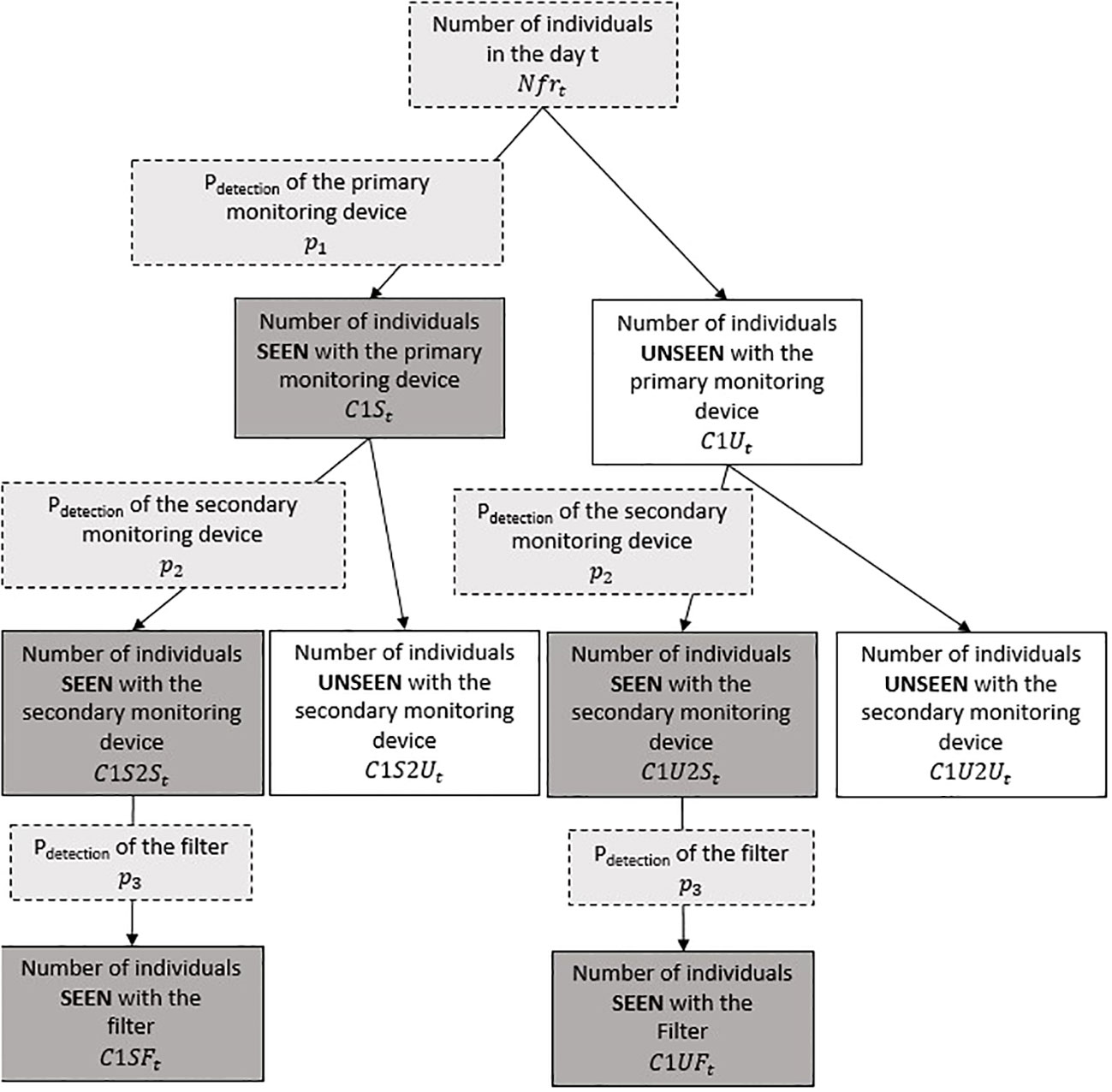
Figure 1 Diagram representing the model structure. Dark gray indicates the data provided to the model, pale gray indicates the parameters and variables of interest that will be estimated, and white indicates the other estimated variables.

2.1.1 The total abundance

The number of fish seen by the primary monitoring device, C1S_t, during a given time step t is modeled as probabilistic issues of binomial experiments. Two underlying hypotheses must be fulfilled: 1) all fish behave independently, and 2) all fish are detected using the same detection probability within a given time step. Under these hypotheses, the number of individuals seen by the primary monitoring device each time step t, C1S_t, is modeled using a binomial distribution with the fish abundance at t Nfr_t and the detection probability of the primary observer p1:

$$C1S_t\sim Binomial(Nf{r}_t,p1)$$

The number of fish seen by the secondary observation device C1S2S_t is modeled using a binomial distribution conditionally on the number of individuals seen on the primary monitoring device C1U2S_t, conditionally on the number of individuals unseen on the primary monitoring device C1U_t, and dependent on the detection probability of the secondary observer p2:

$$C1U_t=Nf{r}_t-C1S_t$$

$$C1S2S_t\sim Binomial(C1S_t,p2)$$

$$C1U2S_t\sim Binomial(C1U_t,p2)$$

The phenology of fish migration depends on species, the geographical position of the environment monitored, and environmental conditions or the time step chosen. As a result, we define the highly variable abundance of fish for each time step, Nfr_t, as follows:

$$Nf{r}_t=round(Yf{r}_t)$$

where Yfr_t is considered to be partially exchangeable and is modeled using a gamma distribution conditionally on the shape r.y_t and the inverse scale mu.y_t.

$$Yf{r}_t= Gamma(r.y_t,mu.y_t)$$

$$r.y_t=\frac{1}{CV.{y_m}^2}$$

$$mu.y_t=\frac{1}{E.y_m\times CV.{y_m}^2}$$

The two parameters $r.y_t$ and $mu.y_t$ are dependent on the expected mean $E.y_m$ and on the coefficient of variation $CV.y_m$ where m $\in$ 1:12 represents a random effect of the month of observation to allow intra-seasonal variability in fish abundance estimates. $E.y_m$ is normally distributed with unknown expected mean, $\mu .E_m$ and standard deviation depending on the month, $\sigma .E_m$ such as:

$$E.y_m\sim Normal(\mu .E_m,\sigma .E_m)$$

The total abundance of fish that migrated by the observation devices over the whole study period is defined as follows:

$$NT=\sum _{t}Nf{r}_t$$

2.1.2 Detection probabilities

The detection probability of the primary and secondary observers depends on the study site and the technology of the observation device. It may also vary over time as a function of environmental conditions (e.g., turbidity). However, there is a potential confounding effect of environmental conditions on fish detection and fish abundance. For instance, flood conditions may result in i) low detection probability of the video counter because of increased turbidity and ii) high fish abundance because high flow triggers migration in, e.g., salmon or eels (Stevens and Miller, 1983; Vøllestad et al., 1986; Bultel et al., 2014; Lebot et al., 2022; Lagarde et al., 2023). Thus, to avoid confusion within the model, we do not account for the environmental covariates, but such an effect could be implemented if needed. The detection probability of the primary and secondary observers where set independently and constant over the study period. A logit scale was used for the detection probabilities. logit(p1) and logit(p2) follow uninformative Normal distributions.

$$logit(p1)\sim Normal(0,0.1)$$

$$logit(p2)\sim Normal(0,0.1)$$

2.1.3 Adding a data pre-processing module to the model

Some observation devices produce continuous recordings of the river, like optic or acoustic cameras. An entire reading of the datasets is highly time-consuming; most studies integrate a pre-processing filter that aims to focus only on observations of fish species of interest. This filter should be set based on known morphological or behavioral characteristics of the target species. The probability of a filter in detecting a fish within the available records may depend on a large number of parameters, such as the diversity and number of fish passages, the clarity of images, the pre-processing algorithm, and the criteria selected to discriminate the species of interest. We thus develop a specific module to describe this specific step of data pre-processing in the model without any a priori knowledge of the pre-processing filter used and estimate its associated specific detection probability p3 (Figure 1). When applying this filter to the second observer (Figure 1), the number of fish seen by the primary observer and detected by the filter, given it was recorded by the secondary observer, C1SF_t, is modeled using a binomial distribution conditionally on the number of fish seen by the primary and secondary observers (C1S2S_t). The detection probability of the filter p3 follows an uninformative Normal distribution. The number of fish unseen by the primary fish counter but seen by the filter after the secondary observer is modeled using a binomial distribution conditionally on the number of fish unseen by the primary observer and seen by the secondary observer (C1U2S_t) and the detection probability of the filter p3.

$$logit(p3)\sim Normal(0,0.1)$$

$$C1S{F}_t\sim Binomial(C1S2S_t,p3)$$

$$C1U{F}_t\sim Binomial(C1U2S_t,p3)$$

To obtain the number of fish seen by the primary observer and secondary observers C1S2S_t and the number of fish unseen by the primary observer and secondary observers C1U2S_t, the operator conducts on a regular basis an exhaustive examination of records from the secondary observer, e.g., without using the pre-processing filter.

2.1.4 Prior specification for free parameters

Prior distributions were assigned to all free parameters (i.e., parameters that are not conditioned by any other quantity of the model). For all, uninformative prior distributions were used in order to let the Bayesian posterior inferences reflect the information brought by the data (Table 1).

Table 1

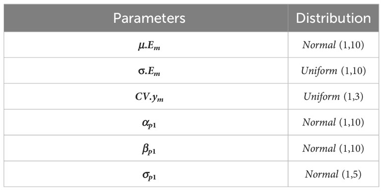
Table 1 Prior distributions of the free parameters.

2.1.5 Computation

We fitted the model within the Bayesian framework using three chains of 300,000 iterations with a burn-in of 270,000 iterations, each with different initial values. We monitored the R ê parameter to assess model convergence (Brooks and Gelman, 1998). We used the R software version 4.2.1 (R Development Core Team, 2022) to simulate the data, and we performed the analyses using the JAGS software from R through the package jagsUI (Kellner, 2021).

2.2 Simulation study

2.2.1 Assessing the limits of the model using simulated datasets

We aimed to test the model to assess its performance at estimating fish run abundance under different conditions of observation. We ran the model using a dedicated set of simulated datasets, simulating daily observation of fish over a period of 1 year, to investigate the effect of 1) the detection probability of each of the two observers; 2) the distribution of observation over time; 3) the total number of observations; 4) the duration of the pairing period, when the two observers are active; and 5) the timing of the pairing period, with regard to the migration phenology.

To ensure biologically reasonable simulations, we built our simulated datasets based on the range of conditions encountered at main French and European fish-counting facilities (Eatherley et al., 2005; Almeida and Rochard, 2015; ICES, 2021; Briand et al., 2022; ICES, 2022), such as the following.

2.2.1.1 Detection probabilities

The detection probability of the fish observation devices is well documented (Fewings, 1992; Reddin et al., 1992; Eatherley et al., 2005) and generally varies between 70% and 100%. The detection probability depends on local site configuration and the species, as one setting would not fit all purposes equally. However, the proportion of migrating fish that do not pass in front of the observation device because of possible bypass is generally unknown. This proportion of escapees is virtually null at large impassable hydropower dams (e.g., in river Perhonjoki for lampreys; Ojutkangas et al., 1995) or extremely high when most of the river flow is diverted into many reaches or when downstream migration can take place through weir spillover. Given these elements, we simulated datasets for detection probabilities of the primary observation device equal to 0.05, 0.2, and 0.7 (three modalities). Assuming that a secondary observation device would be installed in a way to maximize observation of the species of interest, we simulated datasets for detection probabilities of the secondary observation device equal to 0.2 and 0.7 (two modalities) and detection probabilities for the filter equal to 0.2 and 0.7 (two modalities). The list and ID of combinations of detection probabilities are presented in Table 2.

Table 2

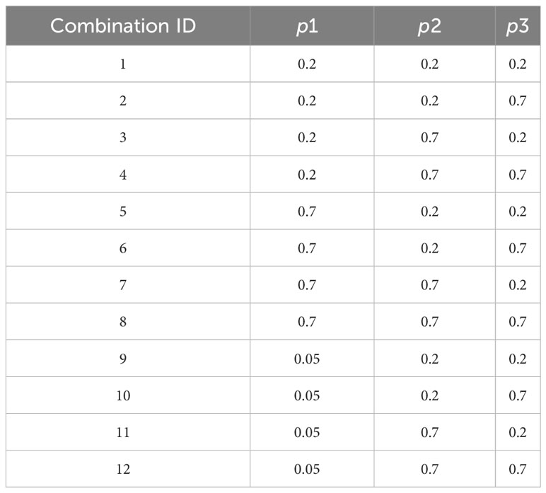
Table 2 Combinations of detection probabilities used to create simulated datasets and their identification numbers.

2.2.1.2 Annual distribution of fish passage

Six diadromous species are mainly targeted at fish counters in Europe: Atlantic salmon (S. salar), sea trout (Salmo trutta), European eel (A. anguilla), shads (Alosa alosa and Alosa fallax spp.), and sea lamprey (Petromyzon marinus). In all these species, the migration phenology is characterized by one or two seasonal peaks of migration when most observations take place (Rochard, 2001; Jonsson & Jonsson, 2002; Orell et al., 2007; Almeida and Rochard, 2015; Sandlund et al., 2017). Thus, we simulated datasets for three modalities derived from the main difference in the migration phenology in those fishes: i) a migration pattern with one peak of fish passage in November, ii) a migration pattern with two peaks of fish passage in July and in November, and iii) a migration pattern with a quasi-homogeneous distribution of fish passage throughout the year with no clear peak, as observed in holobiotic species, as a reference.

2.2.1.3 Annual number of observations by the primary observer

Over the period 2011–2015, most video-counting sites in France recorded between 0 and 200 observations per species of interest annually (Pers. Com. C. Briand). Thus, we selected values of 200, 150, 100, or 50 fish observations for a year ($C1S=\sum C1S_t$) to simulate our datasets (four modalities).

2.2.1.4 Duration of the pairing period

As we aimed to adapt the double-observer approach to situations where the second observer is only operating part of the study time, we tested the effect of the pairing duration on model performance. We simulated periods of three and five consecutive months of paired observations by the two observers (two modalities).

2.2.1.5 Timing of the pairing period

This point is designed to define the best pairing period to set up the temporary secondary observer with respect to the migration phenology and the annual distribution of observations by the primary observer. For this, we simulated independent datasets with a pairing period starting in each month of the year (12 modalities).

2.2.2 Simulation of the datasets

Unique datasets were created for different combinations of the above-mentioned modalities. To create a simulated C1S_t, a random number was generated from a normal distribution with a mean and a standard deviation depending on the month of observation, the seasonal distribution of fish passage, and C1S. The daily abundance of fish passing by the primary observer Nfr_t was simulated by making a random draw in a negative binomial distribution, for which simulated C1S_t and detection probabilities p1 are the parameters. Likewise, during the pairing period, daily observations C1S2S_t and C1U2S_t were simulated by generating a random number from a binomial distribution using simulated detection probabilities p2 and simulated C1S_t or simulated C1U_t = Nfr_t − C1S_t, respectively. Similar procedures were used to simulate C1SF_t and C1UF_t using simulated p3 and simulated C1S2S_t or C1U2S_t as parameters.

We designed a set of simulated datasets, grouped into three experiments, to investigate the performance of the model to the progressive degradation of the information available, such as the following.

2.2.2.1 Experiment 1: the pairing period

We built our simulations starting with modalities of reference depicting the most informative range of conditions that could be expected from most French fish-counting facilities in terms of detection probability (p1 = p2 = p3 = 0.7) and annual number of observations by the primary observer (C1S = 200). We then investigated the effect of the duration and timing of the pairing period on the model output by simulating datasets for pairing periods of 5 and 3 months, for all 12 starting months. We compared the results between the three types of annual distribution of fish passage (n = 72 datasets).

2.2.2.2 Experiment 2: number of observations

Relying on high detection probabilities (p1 = p2 = p3 = 0.7) and low detection probabilities (p1 = p2 = p3 = 0.2), high duration of the pairing period (5 months), and a favorable starting month (as defined in Experiment 1), we simulated a reduction in the annual number of fish observed by the primary observer (C1S = 150, C1S = 100, C1S = 50 respectively). We compared the results between the three types of annual distribution of fish passage and two contrasted sets of detection probabilities (combination IDs 1 and 8, see Table 2) (n = 24 datasets).

2.2.2.3 Experiment 3: detection probabilities

Relying on the high duration of the pairing period (5 months), a favorable starting month (as defined in Experiment 1), and a high annual number of observations by the primary observer (C1S = 200), we simulated a reduction in detection probabilities. We considered all 12 combinations of detection at the primary observer (p1 = 0.05, p1 = 0.2, and p1 = 0.7), detection at the secondary observer (p2 = 0.2 and p2 = 0.7), and detection of the filter (p3 = 0.2 and p3 = 0.7), as defined in Table 2. We compared the results between the three types of annual distribution of fish passage (n = 36 datasets).

In total, we simulated 132 different datasets and ran our model with each dataset to estimate fish run abundance and the detection probabilities. We then assessed the robustness of the model for every dataset by analyzing two types of results: 1) the statistical convergence of the model, which is achieved when the value of $\widehat{R}$ is less than 1.1 (Brooks and Gelman, 1998), and 2) the accuracy of estimates, which is assessed by comparison with the simulated values of the key parameters of the model (detection probabilities p1, p2, and p3 and annual fish run abundance NT). The estimates were considered accurate if their 95% credible interval included the value of the simulated parameters. We selected a pairing period only if the simulated parameters were included within the 95% credible interval of the estimated parameters for all combinations of detection probabilities.

2.3 Case study

The Breuil-en-Auge dam on the Touques River (Normandy, France; coordinates 49.22833188, 0.21336115) was chosen as a study case to estimate the abundance of European eel migrating downstream to the sea. The dam is equipped with a fishway and a fish ladder where a video counter (SYSIPAP computer system, considered as the primary observer) has been operating since 2000. Over the last decade, an average of 230 eels migrating downstream are observed annually, with migration peaking in fall and early winter (Fédération du Calvados pour la pêche et la protection du milieu aquatique, 2015; Fédération du Calvados pour la pêche et la protection du milieu aquatique, 2016; Fédération du Calvados pour la pêche et la protection du milieu aquatique, 2017; Fédération du Calvados pour la pêche et la protection du milieu aquatique, 2018). However, it is suspected that only a small portion of the run is observed and counted because the fishway is likely not efficient in attracting this species on its downstream migration. As shown in Figure 2, eels coming from upstream have several possible routes to migrate downstream: through the fish pass where the video counter is located, through the floodgate gates, or through the diversion reach. An acoustic camera (Adaptive Resolution Imaging Sonar (ARIS), Sound Metrics Corp., Bellevue, WA, USA, considered as the secondary observer) was installed temporarily upstream of all the different pathways (5 m upstream of the fishway entrance toward the video counter) (Figure 2) and recorded continuously the fish moving in its detection beam (1,800-kHz frequency, 5 images per second). The acoustic camera beam was angled to record the greatest proportion of the eels moving downstream the main channel during the period from August 7, 2017, to December 19, 2017. A total of 104 days of simultaneous records (pairing) were retrieved; some records were discarded because of technical issues with the acoustic camera on some days (n = 31). It is known if the operator in charge of analyzing the video records may influence the counts (identification of individuals, identification of species, etc.) (Holmes et al., 2006; Martignac et al., 2015). To avoid variability in operator efficiency, only one experienced operator per device analyzed all the videos. The observation devices were regularly cleaned and returned to their exact position to ensure optimal and stable conditions of visualization.

Figure 2

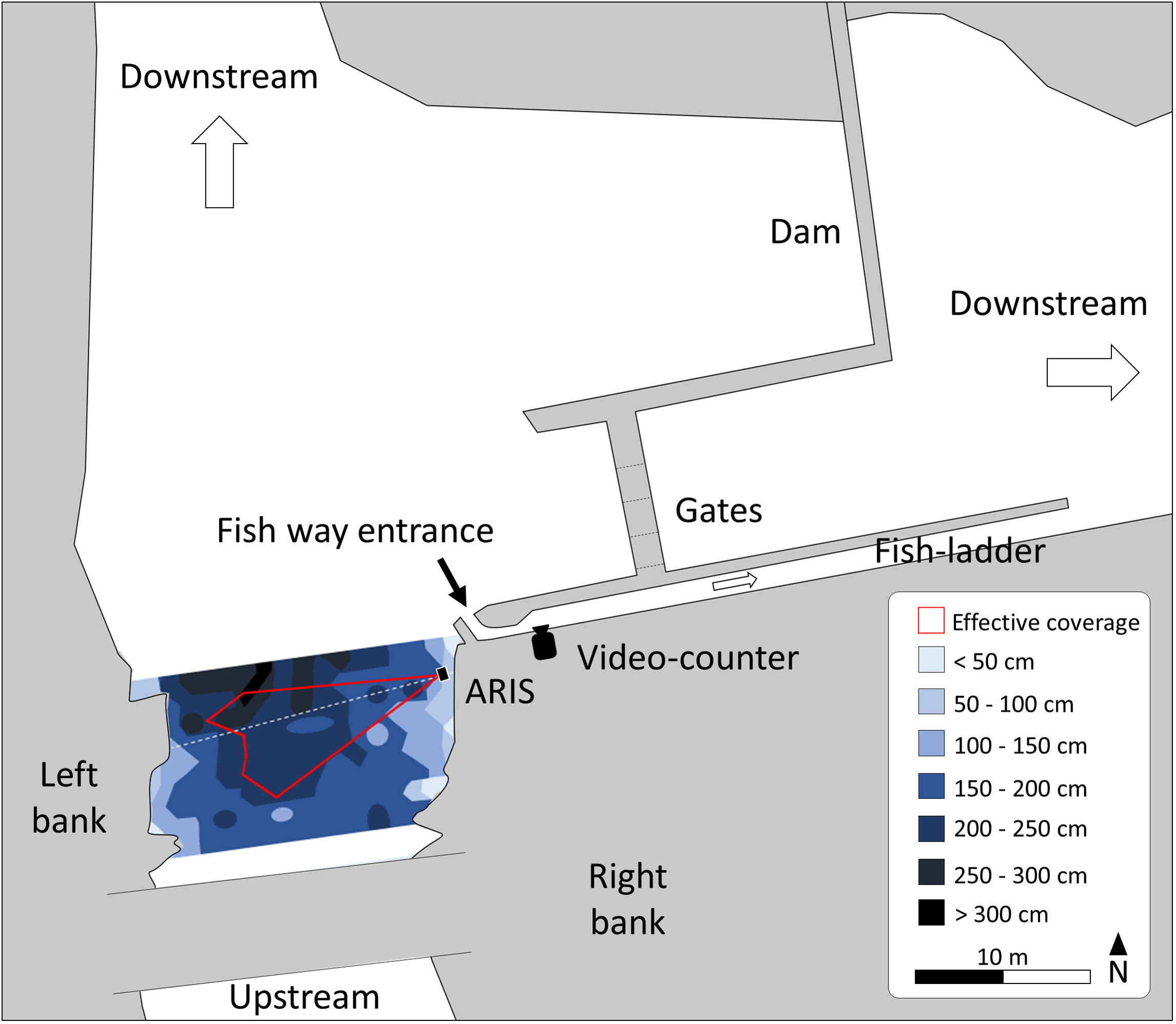
Figure 2 Presentation of the study site, with the localization of the primary and secondary observers.

Because eels mostly migrate at night (Haraldstad et al., 1985), we defined a time step t as a 24-h day starting at 12 a.m. We applied the model to daily observations recorded on both devices. Following the description of the model structure (Figure 1), C1S_t is defined as the daily number of downstream migrating eels seen by the primary observer, which is the video-counting facility. C1SF_t and C1UF_t are daily numbers of eels seen by the filter of the secondary observer (acoustic camera) that were respectively seen and unseen by the primary observer. In this specific case study, the filter consisted of a subset of records from 10 p.m. to 6 a.m., as most eels are known to migrate at nighttime (Haraldstad et al., 1985). To estimate the detection probability of the filter and the detection probability of the acoustic camera, twice a month during the pairing period, the observer counted eels without the filter (seven times during the experiment). This consisted of checking the full daily recordings from 12 a.m. to 12 a.m., C1S2S and C1U2S. Given that a detection probability was defined as the proportion of the fish seen by a specific observer or filter, we considered that missed fish (fish migrating by the observer but not seen) and bypassed fish (fish migrating outside the observer range) were taken into account. We also assumed that the operator was fully efficient in processing the records, which means that he observed all the fish passing by the monitoring device and identified correctly the species of each observed fish. In the absence of individual identification of migrating eel, we assumed that two records of an eel by the primary and secondary observers related to a single individual, if observed within less than 5 minutes, and within the same range of body length ( ± 8 cm, mean size of eels measured with the two devices = 54 cm ± 11 cm. This decision rule allowed us to provide values of C1S_t, C1S2S_t, C1U2S_t, C1SF_t, and C1UF_t as input to the model.

3 Results

3.1 Simulation study

From the two criteria used to assess the robustness of the models, one criterion was met for every model run on simulated data as part of Experiments 1, 2, and 3. The $\widehat{R}$ values were always lower than 1.1 for all parameters, suggesting a good convergence (Brooks and Gelman, 1998). Similarly, the Monte Carlo errors (MC errors) for all parameters were less than 5% of the corresponding posterior standard deviations, supporting a good accuracy of the posterior estimates for all parameters. Below, we describe the performance of the models in terms of based on the accuracy criteria, within each experiment.

3.1.1 Experiment 1: the pairing period

The 95% CI on the total fish abundance NT encompasses the simulated NT in most models; however, only a small number of these models also produced estimates of detection probabilities with good precision (Figure 3). Thus, the structure of the model seems highly sensitive to the selection of the start of the pairing period. This pattern is especially marked for simulated two-peak and holobiotic phenology of fish migration, which appear more difficult to capture by the model than the one-peak phenology of migration. Increasing the duration of the pairing period from 3 months to 5 months generally improves the precision of the model, but it may not always be sufficient to overcome the constraint in the selection of the timing of the pairing period. Among the favorable starting months, we selected September for the one-peak distribution of fish passage and March for the two-peak distribution and holobiotic distribution of fish passage as the starting months of the pairing period to simulate datasets for Experiments 2 and 3.

Figure 3

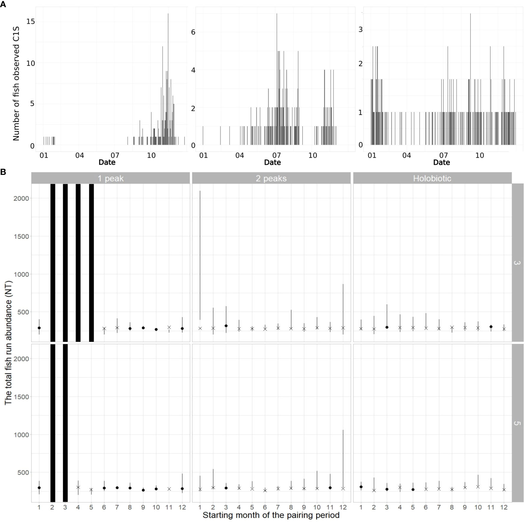
Figure 3 (A) Simulated number of fish observed seen at the primary fish counter (C1S) by annual distribution of fish passages. (B) Assessing the precision of the models in Experiment 1 by comparing the 95% credibility interval on the total fish run abundance (NT, error bars) with the simulated NT. Additional information is provided to specify whether the 95% credibility interval of the estimated detection probabilities (p1, p2, and p3) and NT all encompass the value of the corresponding simulated parameters (dot) or not (cross). Models within Experiment 1 are ordered as a function of the starting month of the pairing period (x-axis), the annual distributions of fish passages (in columns), and the duration of pairing period (in rows). Black bars indicate that no estimates were produced for some starting months, as there was no observation during the entire pairing period.

3.1.2 Experiment 2: number of observations

In general, the precision of the models is little affected by the annual number of fish (Figure 4). Under the range of values simulated in this experiment, the precision of the model is always favorable when C1S_t ≥ 150. In contrast, the precision of the model and the variability in NT estimates improve substantially when the detection probabilities are high. The seasonal distribution of fish passage is again an element affecting the precision of model estimates for any given set of simulated parameters. Results suggest that the model is always more robust at capturing the signal in the data from one-peak migration phenology than in data from two-peak and holobiotic phenologies.

Figure 4

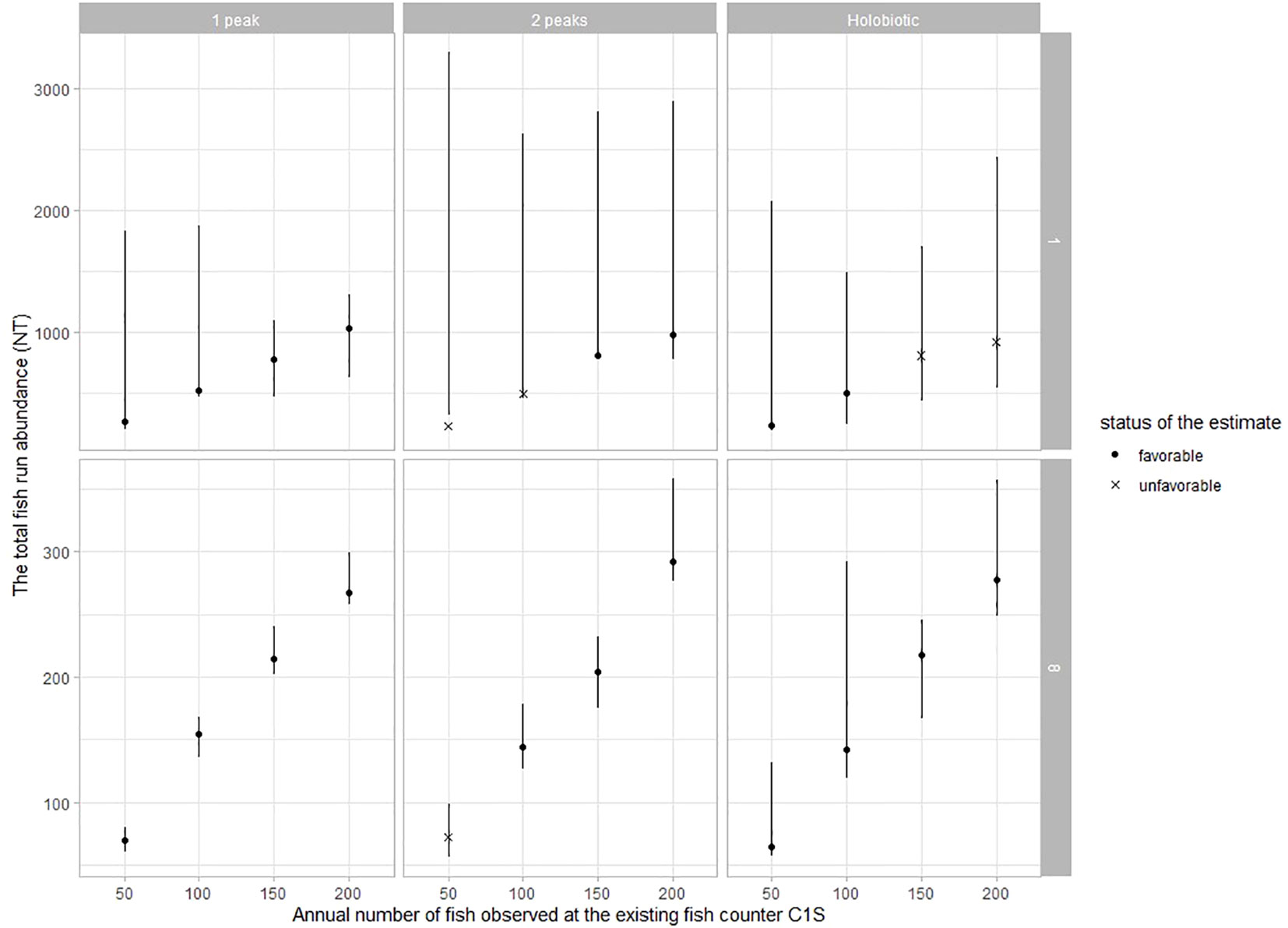
Figure 4 Assessing the precision of the models in Experiment 2 by comparing the 95% credibility interval on the total fish run abundance (NT, error bars) with the simulated NT. Additional information is provided to specify whether the 95% credibility interval of the estimated detection probabilities (p1, p2, and p3) and NT all encompass the value of the corresponding simulated parameters (dot) or not (cross). Models within Experiment 2 are ordered as a function of the annual number of observations by the primary observer (x-axis), the annual distributions of fish passages (in columns), and combinations of detection probabilities (in rows, IDs 1 and 8, see Table 2).

3.1.3 Experiment 3: detection probabilities

By definition, for a given value of C1S_t, the total fish run abundance depends on the detection probability of the primary observer p1 (Figure 5). The accuracy of the model is strongly affected by p1 and to a lesser extent by p2 and p3. The seasonal distribution of fish passage is again an element affecting the accuracy of model estimates. When simulating one-peak and two-peak migration phenologies, the model accurately estimate parameters NT and detection probabilities for all the combinations of detection probabilities, thus making it possible to use the model even when the detection probability of the primary observer is very low (p3 = 0.05). Unfortunately, the data simulated under a scenario of the holobiotic migration phenology appear much more difficult to handle by the model, leading to unfavorable accuracy of the parameter estimates in six out of 10 models.

Figure 5

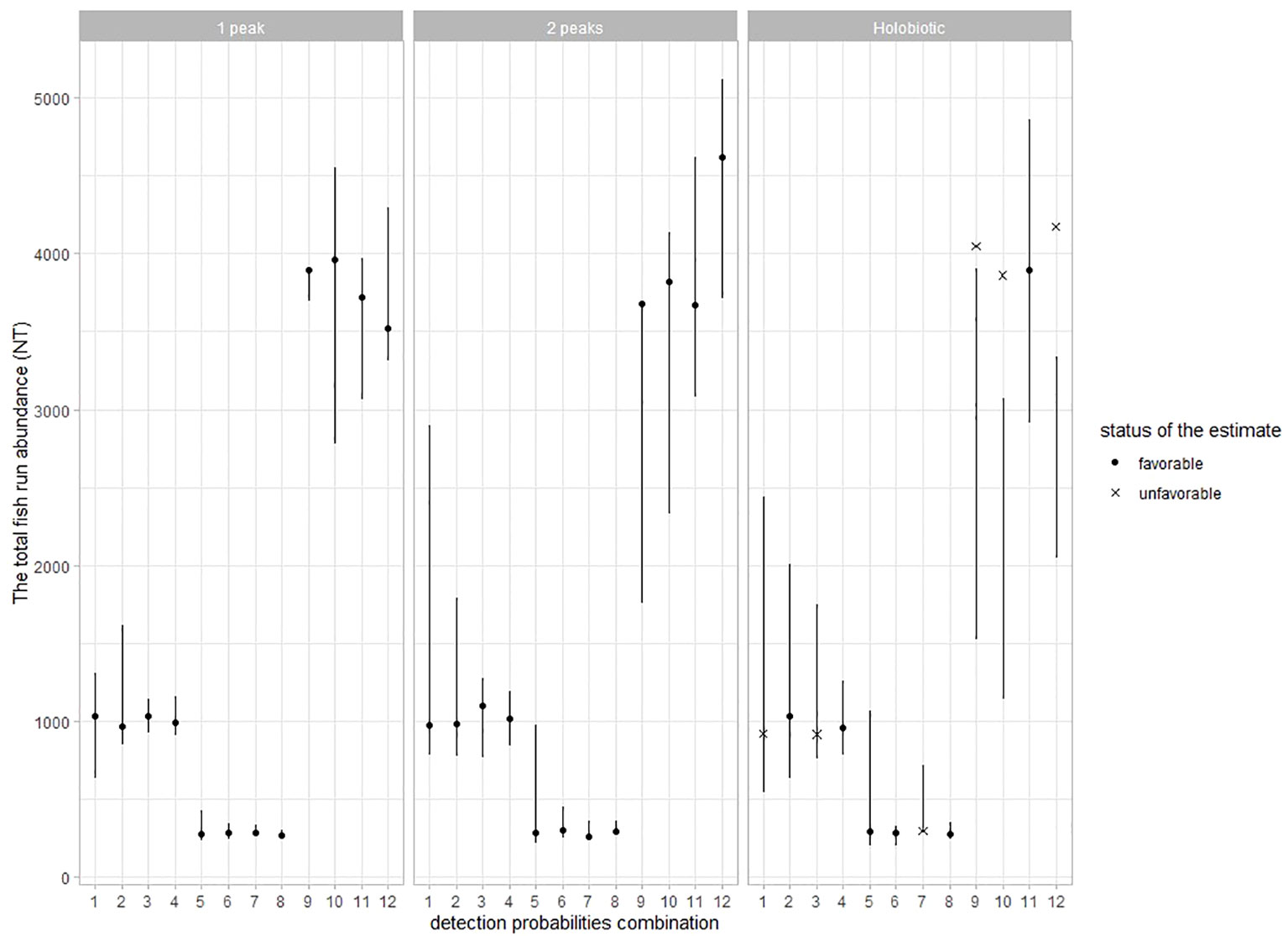
Figure 5 Assessing the precision of the models in Experiment 3 by comparing the 95% credibility interval on the total fish run abundance (NT, error bars) with the simulated NT. Additional information is provided to specify whether the 95% credibility interval of the estimated detection probabilities (p1, p2, and p3) and NT all encompass the value of the corresponding simulated parameters (dot) or not (cross). Models within Experiment 3 are ordered as a function of the combinations of detection probabilities (x-axis, see Table 2) and the annual distributions of fish passages (in columns).

3.2 Case study

At the Breuil-en-Auge fish-counting facility (i.e., the primary observer), 584 migrating eels were seen on the video over the whole 2017 year, which is more than the average (Figure 6A). During the pairing period of 104 days, from August to December 2017, 486 eels were seen on the video counter, and 2,339 eels were seen by the filter of the acoustic camera (secondary observer) (Figure 6B). A 7-day full visualization of the acoustic records was performed without the filter (08/15, 08/30, 09/13, 09/14, 10/19, 10/20, and 11/24), during which 94 eels were seen.

Figure 6

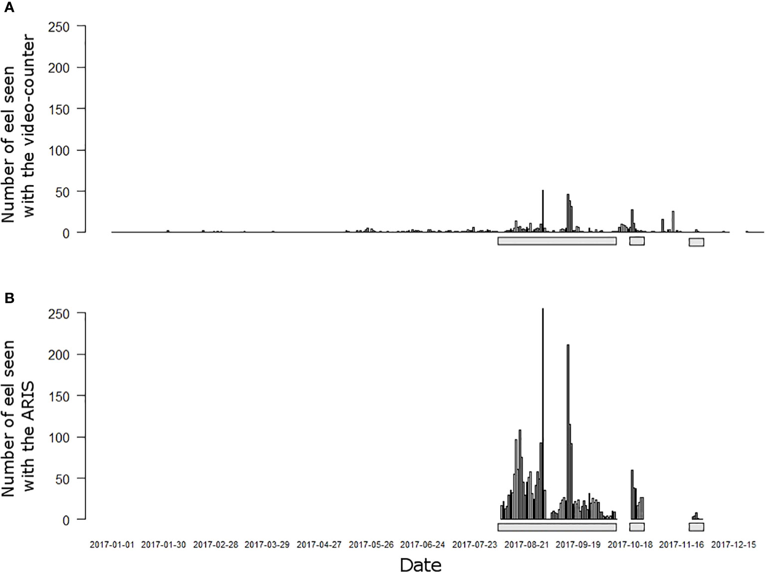
Figure 6 Daily number of observations of European eel at the Breuil-en-Auge fish-counting facility in 2017. Observations (A) by the first observer, the video counter, and (B) by the filter of the second observer, the Adaptive Resolution Imaging Sonar (ARIS) acoustic camera. Gray bars indicate the extent of the pairing period when the two observers were operating simultaneously (n = 104 days).

The model estimated that the detection probability of downstream migrating eels by the Breuil-en-Auge primary observer (fish-counting facility) was p1 = 0.085 (95% credible interval: 0.075–0.095). The secondary observer (acoustic camera) and filter detection probabilities were estimated at p2 = 0.642 (95% credible interval: 0.593–0.690) and p3 = 0.896, respectively (95% credible interval: 0.876–0.915). The distribution of observations was characteristic of a one-peak migration phenology, leading to an estimated annual fish run abundance NT = 6,892 eels (95% credible interval: 6,319–7,559) in 2017 in the Touques River (Figure 7).

Figure 7

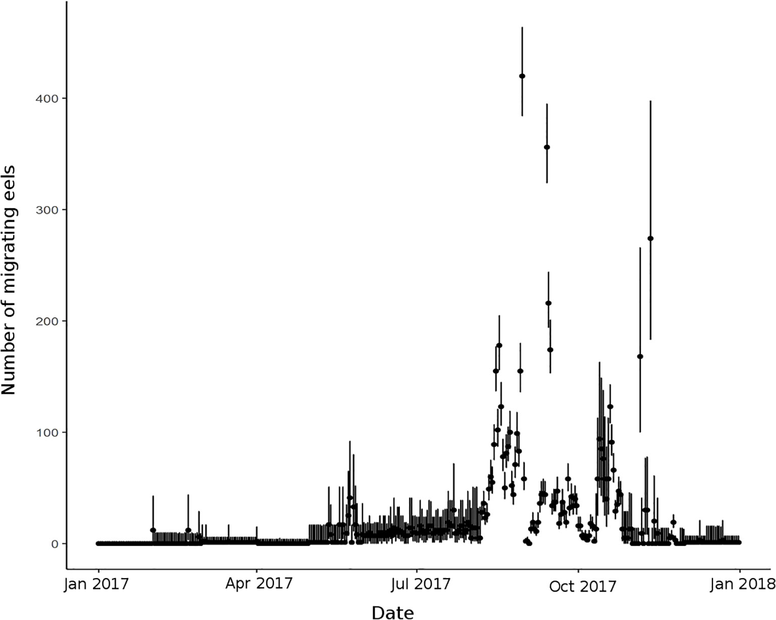
Figure 7 Daily number of migrating eels Nd_t, estimated by the model in the Touques River. Black points represent the estimated median and black lines the 95% credible interval.

4 Discussion

Estimating population abundance is a prerequisite to assess the success of any management action, like the installation of fish ladders or dam removal. Nevertheless, traditional observation systems often provide imperfect counts of individuals and thus fail to accurately quantify changes in abundance in a before–after comparison. In this study, we adopted the double-observer approach to the estimation of the abundance of migrating fish and demonstrated the benefit of temporarily coupling multiple observation systems. Building on three simulation experiments, we provided a detailed investigation of the robustness of our model and discussed the required conditions of its application. In our case study, the use of a nomad equipment as our secondary observer gives support for the generalization of the double-observer approach, with implementation at sites where there is no pre-existing counting device as a perspective.

The analysis of simulated datasets in Experiments 1, 2, and 3 gives evidence that the model can provide robust, accurate, and precise estimates of detection probabilities and total fish abundance in a set of conditions dependent on the information provided in the data. Our results also highlight model limits in estimating key parameters. Throughout the three experiments, we showed that the performance of the model is affected by the seasonal distribution of observations. The model performs well with most datasets simulating a one-peak migration phenology and to a lesser extent datasets simulating a two-peak migration phenology. However, the structure of the model does not seem appropriate to account for observations evenly distributed over the year, as simulated for holobiotic species.

In Experiment 1, we highlighted that the timing of the pairing period is extremely critical. The model achieved its best performance when fed with paired observations encompassing both months of low and high numbers of observations. Setting the pairing period only on the peak months of the migration phenology proved difficult for the model to estimate null daily abundance on days with no observations, which tends to overestimate annual fish run abundance (NT). Similarly, a pairing period running only on months with low or null migration activity tends to underestimate detection probabilities, thus producing inaccurately high numbers of daily migrating fish during the peak of the migration.

In Experiment 2, we tested the effect of a degradation in the information provided by the data on model performance through a reduction in the annual number of observations (and an indirect increase in the number of days with zero observation) as well as a reduction in the detection probabilities. Using datasets simulated for appropriate pairing periods, results indicate that it is possible to estimate NT and detection parameters with favorable precision (simulated values within the 95% credibility interval) even when the information provided by the data decreases. Experiment 2 shows that simulated data with more than 150 fish observed by the primary observer allow reliable estimates of the key parameters. Nevertheless, the uncertainty on parameter estimates (as measured by the 95% credibility interval) increases as the quantity of information in the data decreases.

In Experiment 3, we further investigated how different combinations of detection probabilities p1, p2, and p3 affect the performance of the model. Interestingly, we highlighted that under the simulated conditions, the model can provide reliable estimates for detection probabilities by the first observer as low as 5%. Nevertheless, the uncertainty on parameter estimates (as measured by the 95% credibility interval) increases as the detection probability by the first observer decreases. This low sensitivity of the model to low detection by the primary observer offers a promising avenue to transfer our approach to a wide range of study cases, including temporary settings under potentially suboptimal observation conditions to monitor the abundance of migratory species in the context of dam removal. Our results show that even in this situation, the approach would provide reliable estimates of key parameters as long as the efficiency of the secondary observer is greater than 20% (detection probability below 0.2).

The study on the Touques River has allowed the implementation for the first time of a double-observer approach for the monitoring of a diadromous fish population. It was carried out under the above-defined suitable conditions of application of the model: one-peak migration phenology, a pairing period spanning more than 5 months with more than 200 annual observations by the primary observer, thus illustrating the feasibility of the double-observer approach. As expected for this site, the detection probability of the Breuil-en-Auge fish-counting facility was very low for downstream migrating eels: 0.085 (95% credible interval: 0.075–0.095) in 2017. This estimate is consistent with the configuration of the fishway that was designed for upstream migrating salmonids and proved to be poorly attractive to downstream migrating eels. The filter after the secondary observer, set up to night time, had a detection probability of 0.896, which is consistent with the predominant nocturnal migration of downstream migrating eel. The detection probability of the secondary observer was 0.642. At the time of setting up the secondary observer, we conducted a mapping experiment to evaluate the wetted surface covered by the ARIS. This allowed us to identify that only 20% of the wetted section was covered by the secondary observer (Figure 2). However, the apparent discrepancy between those two numbers can be explained by the active swimming of eels at the bottom of the riverbed under low flow conditions, thus concentrating the migration within the beam of the ARIS. Images recorded by this secondary observer provided further empirical evidence of migratory eels actively swimming at the bottom of the riverbed.

One of the advantages of our methodology is the use of two recording devices. Continuous recording over a long period of time allows us to estimate the total flow of fish throughout the migrating season, rather than just a snapshot of abundance on a given day. This is of great importance for migratory species, especially in the context of a drastic change in their environment such as when a dam is removed (change in water flow, habitats, etc., that can impact their migratory behavior and capacity). However, continuous recording generates a large amount of data, thus requiring substantial resources (staff time) to dedicate to data analysis (Martignac et al., 2015). By implementing a specific module for post-filter data in our model, we can make the most of recent developments in image processing, aiming at limited viewing time. Current advances in deep learning (Fernandez Garcia et al., 2023) are a promising avenue to limit data processing time and make this approach accessible to a larger number of users.

This analysis validated the use of the double-observer method to estimate the fish run abundance of diadromous fish during the year studied and also to estimate historical and future fish run abundance if we consider that the efficiency of the counting system has remained constant over time. However, the assumption of constant detection efficiency is debatable. Detection efficiency potentially depends on the intrinsic characteristics of the counting system and its interaction with the environmental conditions in which it is operated. Excessive turbidity, for example, can have a negative effect on the efficiency of video counting systems by altering the visibility of the counting system (Baumgartner et al., 2012; Soom et al., 2022). In contrast, acoustic cameras are notoriously insensitive to turbidity (Martignac et al., 2015). Accounting for the effect of relevant environmental covariates in modeling time-dependent detection probability (p1_t) would be interesting. If the signal in the data is strong, this improvement may help to decrease the uncertainty around daily abundance estimates Nfr_t and then on the total annual abundance NT. However, as our simulation study has highlighted, further analyses would be needed to identify the benefits and limitations of this approach following such an increase in the complexity of the model. Coupling two counting systems with contrasted characteristics in terms of the detection process may also contribute to overcoming environmental variability.

The application of the double-observer approach under real conditions on the Touques River provides an inspiring illustration of potential gains in quantitative knowledge at monitoring sites. Building on existing facilities, the temporary addition of a secondary observer gives access to valuable estimates of fish run abundance and detection probabilities of fish-counting facilities, which are of key relevance for management. Moreover, our double-observer model offers the potential for wider application settings, e.g., by implementing fully non-permanent monitoring made of two nomad devices. For instance, such a setting could rely on two acoustic cameras on a river where there is no fish-counting facility. In the case of dam removal projects, our model will help estimate diadromous fish population run before and after river continuity restoration. When diadromous fish populations exist on a river catchment, their population increase is taken as a serious argument for dismantling (Duda et al., 2008). Diadromous fish are species of high conservation values and are usually iconic species too, for example, salmon and eel, which have generated a great deal of media attention. In such a case, the gain arising from the continuity restoration program must be clearly addressed.

5 Recommendations

From the combination of simulation experiments and on-field case studies, we identified the minimal requirements for the model to accurately estimate the key parameters of interest and provide technical recommendations to improve data acquisition.

− By definition, the application of the model is only relevant when observation of the target species is imperfect (i.e., escape outside the fish-counting facility is impossible).

− The model can only be applied to observations with marked migration peaks and is not appropriate for the holobiotic type of fish passage. As a consequence, the observation site should be thoroughly selected to monitor active migration while avoiding resting areas or excessive back-and-forth movements that may be generated by the proximity of an obstacle, e.g., dam.

− The target species should be identified without error using both the devices used as the primary and secondary observers.

− A low detection probability by the primary observer (e.g., monitoring device already in place) as long as the total number of annual observations is no less than 150 so that the data are rich enough in information to feed the model.

− For the use of this approach in the field, it is recommended to use simulation datasets corresponding to the case study (phenology) before installing the counting system(s) in order to select the most suitable pairing period and to validate that this methodology can be used.

− The second observer should enable the selected species/stage to be monitored. For example, for the acoustic camera, it is difficult to consider true detection/recognition of individuals smaller than 20 cm unless a very narrow window (<5 m) is recorded (Tušer et al., 2014; Martignac et al., 2015).

− The temporary secondary observer should be installed for a period of five consecutive months so that it covers a large part of the fish migration phenology. It should provide a representative sampling of the fish migration over the duration of the pairing period. If the second observer requires regular handling for maintenance, a system must be put in place to ensure that the device is always in the same position to avoid bias in the data.

− The secondary observation device would ideally be installed in a way that ensures partial overlap with the primary observer, e.g., by pointing at the entrance of the fishway. This setting would allow relieving assumptions for the coupling of individual observations between the primary and secondary observers (e.g., time laps and size matching).

Data availability statement

The raw data for the analysis of the Touques River on european eels are available via this link: https://doi.org/10.57745/6IF2BU. The other raw data for the simulation study will be made available by the authors, without undue reservation.

Ethics statement

Ethical approval was not required for the study involving animals in accordance with the local legislation and institutional requirements because we don’t manipulate animals, just observe them via video.

Author contributions

CB, FM, J-MR, MN, and LB contributed to conception and design of the study. CB and FM created the protocol for collecting the data. CB developed the model and performed the statistical analysis. CB wrote the first draft of the manuscript. J-MR and MN wrote sections of the manuscript. All authors contributed to the article and approved the submitted version.

Funding

The author(s) declare financial support was received for the research, authorship, and/or publication of this article. The study was funded by the French Office for Biodiversity.

Acknowledgments

We are grateful to Y. Salaville and the staff of the Fédération du Calvados pour la pêche et la protection du milieu aquatique for access to the study site and for providing daily observations of eels at the video counter, to JP. Destouches and D. Huteau for their helpful contribution in setting up the acoustic camera at the study site, and to E. Rivot for his invaluable advice during the development of the model.

Conflict of interest

The authors declare that the research was conducted in the absence of any commercial or financial relationships that could be construed as a potential conflict of interest.

Publisher’s note

All claims expressed in this article are solely those of the authors and do not necessarily represent those of their affiliated organizations, or those of the publisher, the editors and the reviewers. Any product that may be evaluated in this article, or claim that may be made by its manufacturer, is not guaranteed or endorsed by the publisher.

References

Aastrup P., Mosbech A. (1993). Transect width and missed observations in counting muskoxen (Ovibos moschatus) from fixed-wing aircraft. Rangifer 13, 99–104. doi: 10.7557/2.13.2.1096

CrossRef Full Text | Google Scholar

Almeida P. R., Rochard E. (2015). Report of the ICES Workshop on Lampreys and Shads (WKLS). (Copenhagen, Denmark: International Council for the Exploration of the Sea).

Google Scholar

Aprahamian M. W., Baglinière J.-L., Sabatié M. R., Alexandrino P., Thiel R., Aprahamian C. D. (2003). “Biology, Status, and Conservation of the Anadromous Atlantic Twaite Shad Alosa fallax fallax,” in Biodiversity, status and conservation of world’s shads American Fisheries Society Symposium. (Bethesda, USA), 23.

Google Scholar

Baumgartner L. J., Bettanin M., McPherson J., Jones M., Zampatti B., Beyer K. (2012). Influence of turbidity and passage rate on the efficiency of an infrared counter to enumerate and measure riverine fish. J. Appl. Ichthyology 28, 531–536. doi: 10.1111/j.1439-0426.2012.01947.x

CrossRef Full Text | Google Scholar

Borchers D. L., Buckland S. ,. T., Zucchini. W. (2002). “Simple mark-recapture,” in Estimating animal abundance. closed populations (London: Springer). doi: 10.1007/978-1-4471-3708-5_6

CrossRef Full Text | Google Scholar

Briand C., Legrand M., Beaulaton L., Boulenger C., Lafarge D., Grall S. (2022)stacomiR: Fish migration monitoring. Available at: https://hal.science/hal-03727236.

Google Scholar

Brooks S. P., Gelman A. (1998). General methods for monitoring convergence of iterative simulations. J. Comput. Graphical Stat 7, 434–455. doi: 10.1080/10618600.1998.10474787

CrossRef Full Text | Google Scholar

Buckland S., Anderson D., Burnham K., Laake J. (1993). Distance Sampling: Estimating Abundance of Biological Populations. Chapman and Hall, London. doi: 10.2307/2532812

CrossRef Full Text | Google Scholar

Bultel E., Lasne E., Acou A., Guillaudeau J., Bertier C., Feunteun E. (2014). Migration behaviour of silver eels (Anguilla Anguilla) in a large estuary of Western Europe inferred from acoustic telemetry. Estuarine Coast. Shelf Sci. 137, 23–31. doi: 10.1016/j.ecss.2013.11.023

CrossRef Full Text | Google Scholar

Chandler R. B., Royle J. A., King D. I. (2011). Inference about density and temporary emigration in unmarked populations. Ecology 92, 1429–1435. doi: 10.1890/10-2433.1

PubMed Abstract | CrossRef Full Text | Google Scholar

Chrysafi A., Kuparinen A. (2016). Assessing abundance of populations with limited data: Lessons learned from data-poor fisheries stock assessment. Environ. Rev. 24, 25–38. doi: 10.1139/er-2015-0044

CrossRef Full Text | Google Scholar

Cook R. D., Jacobson J. O. (1979). A design for estimating visibility bias in aerial surveys. Biometrics 35, 735–742. doi: 10.2307/2530104

CrossRef Full Text | Google Scholar

Core Team R. (2022). R: A Language and Environment for Statistical Computing (Vienna, Austria: R Foundation for Statistical Computing). Available at: https://www.R-project.org/.

Google Scholar

Dail D., Madsen L. (2011). Models for estimating abundance from repeated counts of an open metapopulation. Biometrics 67, 577–587. doi: 10.1111/j.1541-0420.2010.01465.x

PubMed Abstract | CrossRef Full Text | Google Scholar

Desprez M., Crivelli A., Lebel I., Massez G., Gimenez O. (2013). Demographic assessment of a stocking experiment in European Eels. Ecol. Freshw. Fish. 22, 412–420. doi: 10.1111/eff.12035

CrossRef Full Text | Google Scholar

Duda J. J., Freilich J. E., Schreiner E. G. (2008). Baseline studies in the elwha river ecosystem prior to dam removal: introduction to the special issue. nwsc 82, 1–12. doi: 10.3955/0029-344X-82.S.I.1

CrossRef Full Text | Google Scholar

Dunkley D. A., Shearer W. M. (1982). An assessment of the performance of a resistivity fish counter. J. Fish Biol. 20, 717–737. doi: 10.1111/j.1095-8649.1982.tb03982.x

CrossRef Full Text | Google Scholar

Durban J. W., Weller D. W., Lang A. R., Perryman W. L. (2015). Estimating gray whale abundance from shore-based counts using a multilevel Bayesian model. JCRM 15, 61–68. doi: 10.47536/jcrm.v15i1.515

CrossRef Full Text | Google Scholar

Eatherley D., Thorley J., Stephen A., Simpson I., MacLean J., Youngson A. (2005). Trends in Atlantic Salmon: the role of automatic fish counter data in their recording. Scottish Natural Heritage Commissioned Report.

Google Scholar

Farnsworth G. L., Pollock K. H., Nichols J. D., Simons T. R., Hines J. E., Sauer J. R. (2002). A removal model for estimating detection probabilities from point-count surveys. Auk 119, 414–425. doi: 10.1093/auk/119.2.414

CrossRef Full Text | Google Scholar

Fédération du Calvados pour la pêche et la protection du milieu aquatique (2015) Suivi des populations de poissons migrateurs au niveau de la station de contrôle du Breuil-en-Auge. Available at: https://www.federation-peche14.fr/wa_files/rapport%20stacomi%20touques%202015%20aesn-crn-fnpf.pdf.

Google Scholar

Fédération du Calvados pour la pêche et la protection du milieu aquatique (2016) Suivi des populations de poissons migrateurs au niveau de la station de contrôle du Breuil-en-Auge. Available at: https://www.federation-peche14.fr/wa_files/rapport%20stacomi%20touques%202016%20aesn-crn-fnpf.pdf.

Google Scholar

Fédération du Calvados pour la pêche et la protection du milieu aquatique (2017) Station de comptage des poissons migrateurs du Breuil en Auge sur la Touques. Available at: https://www.federation-peche14.fr/wa_files/rapport%20stacomi%20touques%202017%20aesn-crn-fnpf.pdf.

Google Scholar

Fédération du Calvados pour la pêche et la protection du milieu aquatique (2018) Station de comptage des poissons migrateurs du Breuil en Auge sur la Touques. Available at: https://www.federation-peche14.fr/wa_files/rapport%20stacomi%20touques%202018%20aesn-crn-fnpf.pdf.

Google Scholar

Fernandez Garcia G., Corpetti T., Nevoux M., Beaulaton L., Martignac F. (2023). AcousticIA, a deep neural network for multi-species fish detection using multiple models of acoustic cameras. Aquat Ecol 57, 881–893. doi: 10.1007/s10452-023-10004-2

CrossRef Full Text | Google Scholar

Feunteun E. (2002). Management and restoration of European eel population (Anguilla Anguilla): An impossible bargain. Ecol. Eng. 18, 575–591. doi: 10.1016/S0925-8574(02)00021-6

CrossRef Full Text | Google Scholar

Fewings G. A. (1992). Automatic Salmon Counting Technologies + A contemporary review. Atlantic Salmon Trust. Moulin, Pitlochry, Pertshire.

Google Scholar

Figueroa-Pico J., Carpio A. J., Tortosa F. S. (2020). Turbidity: A key factor in the estimation of fish species richness and abundance in the rocky reefs of Ecuador. Ecol. Indic. 111, 106021. doi: 10.1016/j.ecolind.2019.106021

CrossRef Full Text | Google Scholar

Forbes H. E., Smith G. W., Johnstone A. D. F., Stephen A. B. (1999). An assessment of the performance of the resistivity fish counter in the Borland lift fish pass at Lairg Power Station on the River Shin. Fisheries Res. Serv. Rep. 99 (6), 11pp.

Google Scholar

Forsyth D. M., Hickling G. J. (1997). An improved technique for indexing abundance of himalayan thar. New Z. J. Ecol. 21, 5.

Google Scholar

Haraldstad Ø., Vøllestad L. A., Jonsson B. (1985). Descent of European silver eels, Anguilla Anguilla L., in a Norwegian watercourse. J. Fish Biol. 26, 37–41. doi: 10.1111/j.1095-8649.1985.tb04238.x

CrossRef Full Text | Google Scholar

Hard A., Kynard B. (1997). Video evaluation of passage efficiency of american shad and sea lamprey in a modified ice harbor fishway. North Am. J. Fisheries Manage. 17, 981–987. doi: 10.1577/1548-8675(1997)017<0981:VEOPEO>2.3.CO;2

CrossRef Full Text | Google Scholar

Holmes J. A., Cronkite G. M. W., Enzenhofer H. J., Mulligan T. J. (2006). Accuracy and precision of fish-count data from a “dual-frequency identification sonar” (DIDSON) imaging system. ICES J. Mar. Sci. 63, 543–555. doi: 10.1016/j.icesjms.2005.08.015

CrossRef Full Text | Google Scholar

ICES (2021). Joint EIFAAC/ICES/GFCM Working Group on Eels (WGEEL), and Country Reports 2020–2021. (Copenhagen, Denmark: International Council for the Exploration of the Sea). Available at: https://ices-library.figshare.com/articles/report/Joint_EIFAAC_ICES_GFCM_Working_Group_on_Eels_WGEEL_and_Country_Reports_2020_2021/18620876.

Google Scholar

ICES (2022). Working Group on North Atlantic Salmon (WGNAS). (Copenhagen, Denmark: International Council for the Exploration of the Sea). Available at: https://ices-library.figshare.com/articles/report/Working_Group_on_North_Atlantic_Salmon_WGNAS_/19697368.

Google Scholar

IUCN (2022) The IUCN Red List of Threatened Species. Version 2022. Available at: https://www.iucnredlist.org.

Google Scholar

Jonsson N., Jonsson B. (2002). Migration of anadromous brown trout salmo trutta in a norwegian river. Freshw. Biol. 47, 1391–1401. doi: 10.1046/j.1365-2427.2002.00873.x

CrossRef Full Text | Google Scholar

Kellner K. (2021) jagsUI: A Wrapper Around “rjags” to Streamline “JAGS” Analyses. Available at: https://CRAN.R-project.org/package=jagsUI.

Google Scholar

Kéry M., Royle J. A., Schmid H. (2005). Modeling avian abundance from replicated counts using binomial mixture models. Ecol. Appl. 15, 1450–1461. doi: 10.1890/04-1120

CrossRef Full Text | Google Scholar

Kéry M., Schmidt B. (2008). Imperfect detection and its consequences for monitoring for conservation. Community Ecol. 9, 207–216. doi: 10.1556/comec.9.2008.2.10

CrossRef Full Text | Google Scholar

Kissling M. L., Garton E. O., Handel C. M. (2006). Estimating detection probability and density from point-count surveys: a combination of distance and double-observer sampling. Auk 123, 735–752. doi: 10.1642/0004-8038(2006)123[735:EDPADF]2.0.CO;2

CrossRef Full Text | Google Scholar

Lagarde R., Peyre J., Koffi-About S., Amilhat E., Bourrin F., Simon G., et al. (2023). Early or late? Just go with the flow: Silver eel escapement from a Mediterranean lagoon. Estuarine Coast. Shelf Sci. 289, 108379. doi: 10.1016/j.ecss.2023.108379

CrossRef Full Text | Google Scholar

Lebot C., Arago M.-A., Beaulaton L., Germis G., Nevoux M., Rivot E., et al. (2022). Taking full advantage of the diverse assemblage of data at hand to produce time series of abundance: a case study on Atlantic salmon populations of Brittany. Can. J. Fish. Aquat. Sci. 79, 533–547. doi: 10.1139/cjfas-2020-0368

CrossRef Full Text | Google Scholar

Legrand M., Briand C., Besse T. (2019). stacomiR: a common tool for monitoring fish migration. J. Open Source Software 4, 791. doi: 10.21105/joss.00791

CrossRef Full Text | Google Scholar

Limburg K. E., Waldman J. R. (2009). Dramatic declines in north atlantic diadromous fishes. BioScience 59, 955–965. doi: 10.1525/bio.2009.59.11.7

CrossRef Full Text | Google Scholar

Mallet D., Pelletier D. (2014). Underwater video techniques for observing coastal marine biodiversity: A review of sixty years of publication, (1952–2012). Fisheries Res. 154, 44–62. doi: 10.1016/j.fishres.2014.01.019

CrossRef Full Text | Google Scholar

Marques T. A., Buckland S. T., Borchers D. L., Tosh D., McDonald R. A. (2010). Point transect sampling along linear features. Biometrics 66, 1247–1255. doi: 10.1111/j.1541-0420.2009.01381.x

PubMed Abstract | CrossRef Full Text | Google Scholar

Martignac F., Daroux A., Bagliniere J.-L., Ombredane D., Guillard J. (2015). The use of acoustic cameras in shallow waters: new hydroacoustic tools for monitoring migratory fish population. A review of DIDSON technology. Fish Fisheries 16, 486–510. doi: 10.1111/faf.12071

CrossRef Full Text | Google Scholar

McGill B. J. (2010). Matters of scale. Science 328, 575–576. doi: 10.1126/science.1188528

PubMed Abstract | CrossRef Full Text | Google Scholar

McShea W. J., Forrester T., Costello R., He Z., Kays R. (2016). Volunteer-run cameras as distributed sensors for macrosystem mammal research. Landscape Ecol. 31, 55–66. doi: 10.1007/s10980-015-0262-9

CrossRef Full Text | Google Scholar

Nichols J. D., Hines J. E., Sauer J. R., Fallon F. W., Fallon J. E., Heglund P. J. (2000). A double-observer approach for estimating detection probability and abundance from point counts. Auk 117, 393–408. doi: 10.2307/4089721

CrossRef Full Text | Google Scholar

Ojutkangas E., Aronen K., Laukkanen E. (1995). Distribution and abundance of river Lamprey (Lampetra fluviatilis) ammocoetes in the regulated river Perhonjoki. Regulated Rivers: Res. Manage. 10, 239–245. doi: 10.1002/rrr.3450100218

CrossRef Full Text | Google Scholar

Orell P., Erkinaro J., Svenning M. A., Davidsen J. G., Niemelä E. (2007). Synchrony in the downstream migration of smolts and upstream migration of adult Atlantic salmon in the subarctic River Utsjoki. J. Fish Biol. 71, 1735–1750. doi: 10.1111/j.1095-8649.2007.01641.x

CrossRef Full Text | Google Scholar

Ouellet V., Collins M. J., Kocik J. F., Saunders R., Sheehan T. F., Ogburn M. B., et al. (2022). The diadromous watersheds-ocean continuum: Managing diadromous fish as a community for ecosystem resilience. Front. Ecol. Evol. 10. doi: 10.3389/fevo.2022.1007599

CrossRef Full Text | Google Scholar

Reddin D. G., O’connell M. F., Dunkley D. A. (1992). Assessment of an automated fish counter in a Canadian river. Aquaculture Res. 23, 113–121. doi: 10.1111/j.1365-2109.1992.tb00601.x

CrossRef Full Text | Google Scholar

Reidy J. L., Thompson F. R. III, Bailey J. W. (2011). Comparison of methods for estimating density of forest songbirds from point counts. J. Wildlife Manage. 75, 558–568. doi: 10.1002/jwmg.93

CrossRef Full Text | Google Scholar

Renaud C. B. (1997). Conservation status of Northern Hemisphere lampreys (Petromyzontidae). J. Appl. Ichthyology 13, 143–148. doi: 10.1111/j.1439-0426.1997.tb00114.x

CrossRef Full Text | Google Scholar

Rivot E., Prévost E. (2002). Hierarchical Bayesian analysis of capture-mark-recapture data. Can. J. Fish. Aquat. Sci. 59, 1768–1784. doi: 10.1139/f02-145

CrossRef Full Text | Google Scholar

Rivot E., Prévost E., Cuzol A., Baglinière J.-L., Parent E. (2008). Hierarchical Bayesian modelling with habitat and time covariates for estimating riverine fish population size by successive removal method. Can. J. Fish. Aquat. Sci. 65, 117–133. doi: 10.1139/f07-153

CrossRef Full Text | Google Scholar

Robinson R. A., Crick H. Q. P., Learmonth J. A., Maclean I. M. D., Thomas C. D., Bairlein F., et al. (2009). Travelling through a warming world: climate change and migratory species. Endangered Species Res. 7, 87–99. doi: 10.3354/esr00095

CrossRef Full Text | Google Scholar

Rochard E. (2001). Migration anadrome estuarienne des géniteurs de grande alose alosa alosa, allure du phénomène et influence du rythme des marées. Bull. Français la Pêche la Pisciculture, 853–867. doi: 10.1051/kmae:2001023

CrossRef Full Text | Google Scholar

Roper B., Scarnecchia D. L. (2000). Key strategies for estimating population sizes of emigrating salmon smolts with a single trap. Rivers 7, 77–88.

Google Scholar

Royle J. A. (2004). N-mixture models for estimating population size from spatially replicated counts. Biometrics 60, 108–115. doi: 10.1111/j.0006-341X.2004.00142.x

PubMed Abstract | CrossRef Full Text | Google Scholar

Royle J. A., Dorazio R. M. (2006). Hierarchical models of animal abundance and occurrence. . JABES 11, 249–263. doi: 10.1198/108571106X129153

CrossRef Full Text | Google Scholar

Runge C. A., Martin T. G., Possingham H. P., Willis S. G., Fuller R. A. (2014). Conserving mobile species. Front. Ecol. Environ. 12, 395–402. doi: 10.1890/130237

CrossRef Full Text | Google Scholar

Sandlund O. T., Diserud O. H., Poole R., Bergesen K., Dillane M., Rogan G., et al. (2017). Timing and pattern of annual silver eel migration in two European watersheds are determined by similar cues. Ecol. Evol. 7, 5956–5966. doi: 10.1002/ece3.3099

PubMed Abstract | CrossRef Full Text | Google Scholar

Servanty S., Prévost É. (2016). Mise à jour et standardisation des séries chronologiques d’abondance du saumon atlantique sur les cours d’eau de l’ORE DiaPFC et la Bresle. (Rennes: ONEMA-INRA).

Google Scholar

Soom J., Pattanaik V., Leier M., Tuhtan J. A. (2022). Environmentally adaptive fish or no-fish classification for river video fish counters using high-performance desktop and embedded hardware. Ecol. Inf. 72, 101817. doi: 10.1016/j.ecoinf.2022.101817

CrossRef Full Text | Google Scholar

Stevens D. E., Miller L. W. (1983). Effects of river flow on abundance of young chinook salmon, american shad, longfin smelt, and delta smelt in the sacramento-san joaquin river system. North Am. J. Fisheries Manage. 3, 425–437. doi: 10.1577/1548-8659(1983)3<425:EORFOA>2.0.CO;2

CrossRef Full Text | Google Scholar

Suryawanshi K. R., Bhatnagar Y. V., Mishra C. (2012). Standardizing the double-observer survey method for estimating mountain ungulate prey of the endangered snow leopard. Oecologia 169, 581–590. doi: 10.1007/s00442-011-2237-0

PubMed Abstract | CrossRef Full Text | Google Scholar

Thibault M. (1987). “Eléments de la problématique du saumon Atlantique en France,” in La restauration des rivières à saumon (Paris: INRA Editions), 413–425.

Google Scholar

Tušer M., Frouzová J., Balk H., Muška M., Mrkvička T., Kubečka J. (2014). Evaluation of potential bias in observing fish with a DIDSON acoustic camera. Fisheries Res. 155, 114–121. doi: 10.1016/j.fishres.2014.02.031

CrossRef Full Text | Google Scholar

Vøllestad L. A., Jonsson B., Hvidsten N. A., Næsje T. F., Haraldstad Ø., Ruud-Hansen J. (1986). Environmental factors regulating the seaward migration of european silver eels (Anguilla Anguilla). Can. J. Fish. Aquat. Sci. 43, 1909–1916. doi: 10.1139/f86-236

CrossRef Full Text | Google Scholar

Williams B. K., Nichols J. D., Conroy M. J. (2002). Analysis and management of animal populations (San Diego, CAAcademic Press).

Google Scholar

Wyatt R. J. (2002). Estimating riverine fish population size from single- and multiple-pass removal sampling using a hierarchical model. Can. J. Fish. Aquat. Sci. 59, 695–706. doi: 10.1139/f02-041

CrossRef Full Text | Google Scholar