Climate factors drive plant distributions at higher taxonomic scales and larger spatial scales

Introduction: Understanding the environmental effects shaping plant distributions is crucial for predicting future ecosystems under climate change. The effects of different environmental factors may vary in their importance in determining plant distributions at different spatial and taxonomic scales, which affects our understanding of plant–environment relationships. However, this has not yet been systematically explored.

Methods: Here we combined global distribution data of 205 widely distributed plant families and environmental data from multiple global databases. We then used the random forest algorithm to quantify the relative importance of environmental factors (including climate, soil, and topography) on the distribution of plants at three taxonomic levels (family, genus, and species) and multiple spatial scales (10 spatial extents from 1° × 1° to 10° × 10° randomly located across the globe). Mixed-effect models were used to assess the significance of spatial and taxonomic scales on relative environmental effects across the globe.

Results: We found that climate factors had increasing importance on plant distributions at higher taxonomic scales and larger spatial scales (yet stochastic effects at spatial extents finer than 4° × 4°). Edaphic factors congruously decreased their importance on plant distributions as spatial and taxonomic scales increased. Topographic factors had a relatively larger influence at higher taxonomic levels (i.e., family>genus>species), but with a relatively slow rise with the increase in spatial scale.

Discussions: Our findings are generally aligned with current knowledge but have also indicated the potential complexity underlying the scale-dependence of relative environmental effects on plant distributions. Overall, we highlight a multi-scale insight into ecological patterns and underlying mechanistic processes.

Introduction

Disentangling how environmental factors drive plant distribution across the globe is crucial for understanding how plants may respond to climate change (Guisan & Thuiller, 2005; Elith & Leathwick, 2009). Generally, abiotic environmental factors are believed to restrict plant ranges since they define the basic conditions for survival (e.g., fundamental niches; Hutchinson, 1957), while finer-scale habitat heterogeneities and biotic interactions further constructure their real distribution patterns (Smith & Read, 1997; Davies et al., 2005; Callaway, 2007; Lin et al., 2013). Research scales may define the range of observations of patterns and processes, thereby influencing our interpretation of ecological questions (Wiens, 1989; Crawley & Harral, 2001; Siefert et al., 2012; Chave & Bascompte, 2013; Viana & Chase, 2019). However, many studies have been conducted at specific spatial or taxonomic scales (Yackulic & Ginsberg, 2016). Our former research on the environmental drivers of global plant distributions found that different environmental factors shape plant distributions in different extent at global and regional scales, varying their importance across latitudes and among taxonomic groups (Huang et al., 2021). Although there have been various studies on the effects of different environmental factors on plant distributions at varying scales in the last decade (Woodward & Williams, 1987; Münzbergová, 2004; Woodward et al., 2004; Siefert et al., 2012; Schweiger & Beierkuhnlein, 2016), the general rule of how different environmental effects on plant distributions change at different scales still requires systematically quantification.

Environmental factors often vary in their heterogeneity at different spatial scales, which may lead to the scale dependency of environmental effects on plant distributions from a macroecological perspective. For example, climate factors often show larger heterogeneity at the global scale than at the regional scale (e.g., within a city or a state) (Perlwitz et al., 2017), while edaphic variables are always varying at fine spatial scales. The scale-dependence of environmental heterogeneity may influence our detection of plant–environment relationships at broad scales. A meta-analysis explored the scale-dependence of vegetation–environment relationship (Siefert et al., 2012), yet it was unable to give a quantitative description of how different effects vary specifically across scales.

The taxonomic scale of observations also influences plant distribution patterns, which has been little investigated until recently (Cox and Moore, 1985; Queenborough et al., 2009; Graham et al., 2018; Yeh et al., 2019). The taxonomic level of the studied object may influence the spatial extent of analysis (by changing the sample size). For instance, a widely distributed family can contain wide- and narrow-range genera or species, and therefore the plant–environment relationship (which is sensitive to their geographical ranges) may change when shifting from a family to a genera/species within it (see the example of Asteraceae in Cox and Moore, 1985). More importantly, taxonomic scales are related to phylogenetic history (Graham et al., 2018) and may reflect the effects of evolutionary events on ecological patterns to some extent. For example, factors induced by long-term history on earth (e.g., climate change through glacial epochs) may influence plant distributions at the early age of speciation, resulting in variations among larger taxonomic scales (e.g., family > species). Conversely, ecological processes such as soil erosion and nutrient turnover may influence plant distributions at a relatively recent period, leading to higher impacts at a finer scale.

It is widely recognized that climate conditions generally shape the current patterns of vegetation across the globe (e.g., Von Humboldt, 1805; Woodward & Williams, 1987). Climatic variables show larger heterogeneity at broad spatial scales, which indicates a stronger effect of climate on plant distributions as spatial scale increases. Moreover, climate has affected plant distributions over long evolutionary history by limiting plant dispersal within specific climate zones across the globe (Woodward et al., 2004) and by influencing their adaptation and speciation under climate change (Levin, 2019). Thus, plants’ responses to climate are more likely to be detected at higher taxonomic scales (e.g., family > species). Thus, relative effects of climate may increase with spatial and taxonomic scales.

Soil heterogeneity tends to occur at smaller spatial scales compared with climate (Weil & Brady, 2017), indicating that soil effects may happen at relatively fine spatial extents. Soil properties determine the nutrients and microbial activities that are important for plant growth and dispersal, usually at a small scale (Jamir et al., 2019; Martinez-Almoyna et al., 2020). These activities occurred within a relatively short period in the history of earth. Thus, soil variables are more likely to affect plant distributions at lower taxonomic levels. In general, we can hypothesize that soil effects increase with both decreasing spatial and taxonomic scales. However, studies on plant–soil relationships have typically focused on community scales, with less attention on large-scale patterns (Marage & Gégout, 2009; Ni & Vellend, 2024). Understanding how soil influences change with scale can contribute to predictions of large-scale species distribution and diversity patterns (Beauregard & de Blois, 2014).

Topographical factors have both direct (e.g., forming geographical barriers at higher spatial extents across the landscape) and indirect effects (e.g., shaping elevational microclimate and soil conditions at regional and local scales) on plant distribution (Lomolino, 2001; Barry, 2008). They are more likely to influence montane taxa than lowland ones because mountain ecosystems contain much more variation in topographic conditions and other related changes in climate and soil. Therefore, the influence of spatial extent may diminish when it is beyond mountain ranges. Geographic isolation arising from topography may cause the allopatric divergence and speciation of related species distributed in mountain and lowland areas (Vargas et al, 2020). Hence, the variations in the response of plants to topography are more likely to be remarkable at the species level than at the family level.

To explore how environmental factors shape plant distributions at different spatial and taxonomic scales, we studied global plant distributions. First, we assessed the impacts of climate, soil, and topography on plant distributions using the random forest algorithm for wide-ranging plants at varying scales. We then used mixed effect models to analyze the effects of the spatial and taxonomic scales of different environmental variables on plant distributions. Through these, we aimed to test our hypotheses: climatic factors have greater importance on plant distributions with increasing spatial scales and at higher taxonomic scales (H1), while edaphic factors have the opposite trends, i.e., increasing influence at finer spatial and taxonomic scales (H2). Topography has a stronger effect at higher taxonomic scales (H3) but limited influence along spatial scales. By quantifying plant–environment patterns across scales, we attempt to provide a macroecological perspective on the changes in ecological patterns and processes with scales.

Methods

Plant distribution data and environmental variables

We collected species occurrence information (species presence data with geographical coordinates) from the Global Biodiversity Information Facility (GBIF, http://www.gbif.org/; data accessed in 2021) database, using family names in The Plant List (TPL, http://www.theplantlist.org/).¹ Then we used the “CoordinateCleaner” R package to clean the original occurrence data, discarding coordinates that matched the centroids of countries, capitals, known botanical institutions, and GBIF headquarters, zero coordinates and equal latitude and longitude, as well as those falling in the sea (Zizka et al., 2019). We also excluded occurrences where geographical information was missing or duplicated. We then selected widely distributed families, which were distributed in at least the main continents (excluding Antarctica) and across a wide range of latitudes (spanning more than ninety degrees). We focused on wide-ranging families because narrow-ranging plant groups were likely to have restricted ranges, and so their responses to the environment might be simplified across scales or may not be detected at varying spatial scales. We ultimately obtained 205 families, 688 genera, and 1610 species for the subsequent analyses (Supplementary Information Appendix S2).

We obtained information on climatic, topographic, and soil variables, which are crucial in determining plant distributions at multiple scales. Temperature and precipitation variables were derived from WorldClim (http://www.worldclim.org/). Solar radiation was obtained from Global Solar Alta 2.0 (https://globalsolaratlas.info/).² We collected the properties of topsoil (e.g., total nitrogen, pH) from two databases, the Harmonized World Soil Database (HWSD; https://www.fao.org/soils-portal/data-hub/soil-maps-and-databases/harmonized-world-soil-database-v12/en/; Fischer et al., 2008) and the Global Soil Database (http://globalchange.bnu.edu.cn/research/soilw; Shangguan et al., 2014). We derived topographic variables (i.e., elevation, aspect, and slope) from the Advanced Spaceborne Thermal Emission and Reflection Radiometer (ASTER) Global Digital Elevation Model (GDEM). All the environmental variables (Supplementary Information Appendix S1: Table S1.1) were processed into 30 arc-second rasters, and the values were extracted according to the geographical locations of the corresponding plant taxa. We conducted principal component analysis (PCA) for variables from the same resource (e.g., temperature and precipitation from WorldClim) or of similar type (e.g., soil properties from two databases) to avoid spurious collinearity among original variables and to reduce environmental dimensions for subsequent analyses. For 19 climate variables (indexes about temperature and precipitation) in worldClim, we used the first three principal components (PCs)that accounted for > 80% of the variance. For 15 soil variables, we used the first five soil PCs. which accounted for > 70% in soil variables (Supplementary Information Appendix S1: Tables S1.3, S1.4). We ultimately obtained 12 environmental variables (including eight PC axes) for subsequent analysis (Supplementary Information Appendix S1: Table S1.2).

Random locations, spatial and taxonomic scales

We assessed the effects of spatial scales based on different spatial extents at the regional scale. We first randomly sampled 500 locations across the globe (Figure 1). These locations distribute across all the main continents and cover most ecological biomes (both Whittaker biomes, Whittaker, 1975, and WWF biomes, Olson et al., 2001; Supplementary Information Appendix S1: Figure S1.1). Frequents of different biomes were not same due to varying areas of these biomes across the globe and different data density in GBIF database (even when we have conducted data manipulation to reduce sample bias). Then, we created “plots” around the center of each location, spanning 1° × 1°, 2° × 2°, 3° × 3°, 4° × 4°, 5° × 5°, 6° × 6°, 7° × 7°, 8° × 8°, 9° × 9°, or 10° × 10° (i.e., 10 levels of spatial extents at the regional scale). We considered all occurrences of a plant taxon (only at the family, genus, or species level) in each plot with a specific spatial extent as an individual dataset. In this case we can analyze scales effect by controlling the locations (as random effects in the mixed effect model below). Plant taxa with less than three occurrences within a sampled plot were removed from the datasets. We further selected the plots with at least three taxonomic groups at the corresponding taxonomic scale to satisfy the random forest analysis. We focused on the extent instead of the grain because plant occurrence was obtained as scattered data (with geographical coordinates) and was processed to the same resolution as environmental variables. For a comparison at a specific location, we assessed the difference in relative environmental effects across 10 levels of spatial extents and 3 levels of taxonomic ranks.

Figure 1

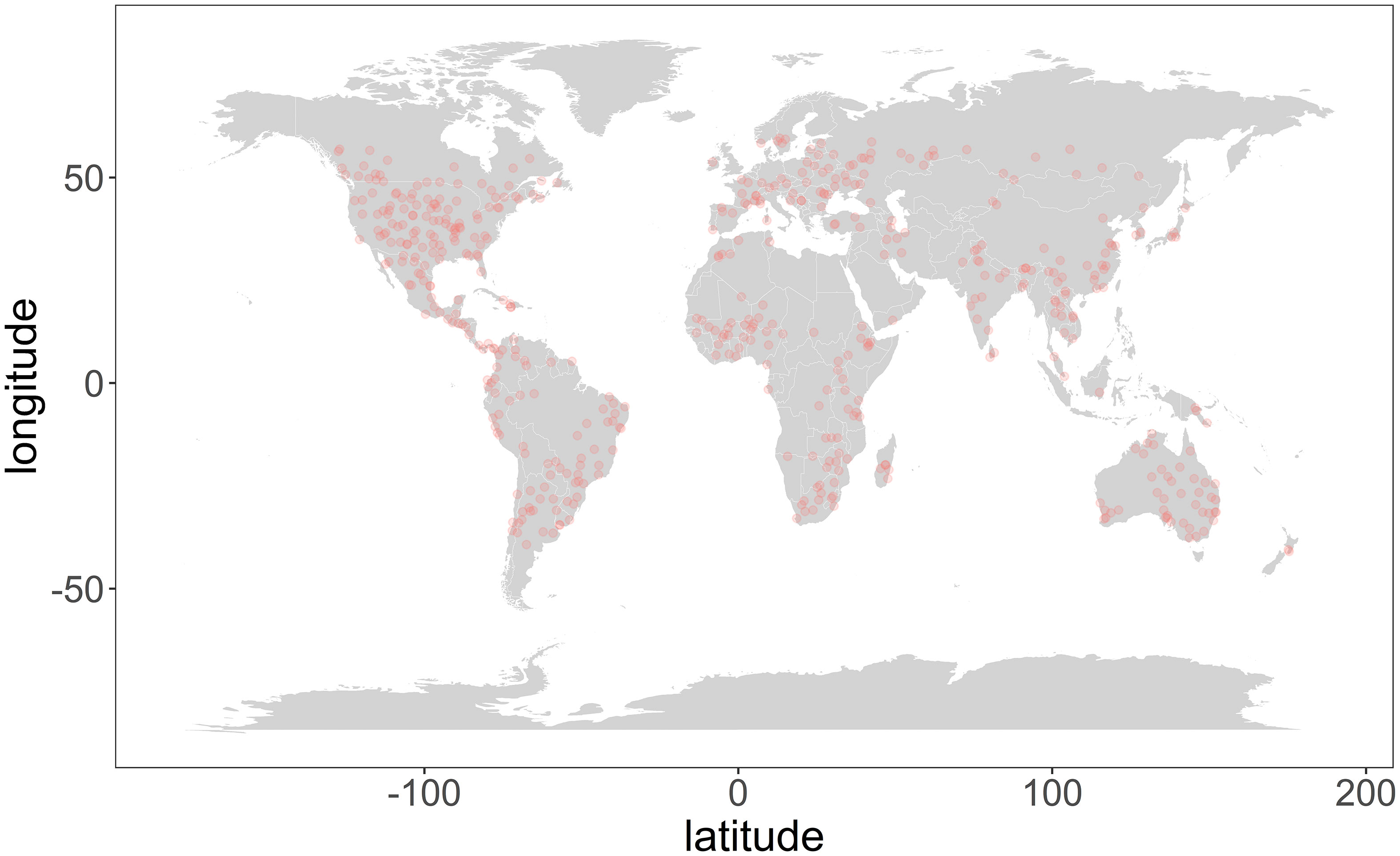
Figure 1 Distribution of 500 plots randomly selected across the globe.

Relative importance of environmental factors

We used random forest to assess the relative importance of the environmental factors affecting plant distribution at multiple scales. The random forest algorithm is a combination of tree predictors, where each tree relies on the values of a random vector that are sampled independently and with the same distribution for all trees in the forest (Breiman, 2001). It is more precise and applicable when dealing with large multivariate data (nonlinear, correlated, or biased) than classical statistical methods, and hence it is widely used in classification and regression, especially the selection of variables in ecology (Cutler et al., 2007; Genuer et al., 2010). We conducted random forest for every dataset (species data at one particular spatial and taxonomic scale in a location) separately. In each random forest model, we used presence–absence of 0.5° × 0.5° grid cells as dependent variables, and associated environmental variables (12 variables in every grid corresponding to occurrence) as explanatory variables. Presence points were defined as occurrence records of a plant taxon (at family, genus, or species levels), while absence points were represented by the same number of presence points (pseudo-absences) that were randomly selected from background grid cells for every focal taxon (Barbet-Massin et al., 2012). Datasets with less than three occurrences were excluded due to the requirements of random forest.

We performed random forest algorithms using the “randomForest” package in R 3.6.1 (Liaw & Wiener, 2002). The random forest takes bootstrapped samples from the original dataset to build a decision tree, and then average the predictions of each tree for a final model. The number of sampled trees in our study was set to 500 for every test. We used the mean decrease Gini (MDG) to assess the relative contribution of every environmental factor. It measures the total decrease in node impurities (averaged over all trees) from splitting on the variable, so it reflects the overall importance of every variable from the model. Larger MDG values indicate greater importance (Hong et al., 2016). We calculated the MDG value for every environmental factor at every spatial and taxonomic scales. To facilitate comparison among datasets of different scales, we standardized the MDG values to the range of 0 to 1 in every dataset using the equation MDG_{Standardized,i} = MDG_i/(${\displaystyle {\sum }_i^{15}MD{G}_i}$). For species occurring in the same location at the same spatial and taxonomic scale, we conducted the random forest algorithm separately for every species (or genus or family) taxon respectively. Thus, we obtained over 15000 datasets at different spatial and taxonomic scales to run random forest in total.

To evaluate the model performance, we used the out of bag (OOB) error rates from random forest model. It is an estimate of error rate, calculated as (1 – accuracy), which means that lower OOB indicated higher accuracy. We also calculated the cross-validation out of bag (CV OOB) error rates as supplementary, using “rf.crossValidation” functions in “rfUtilities” R package (Evans & Cushman, 2009).

Mixed effect models

We used mixed effect models to test the effects of spatial and taxonomic scales on the relative importance of environmental factors (represented as MDG values of every variable at specific scales from the random forest). We performed different models for three types of variables (climate, soil, and topography) and for every single factor (12 variables, including PCs). First, we classified the environmental variables into three groups (i.e., climate, soil, and topography) and conducted the analysis separately for each group. For each group, we added all variables’ relative importance (e.g., the sum of relative importance of all three climate PCs and solar radiation) at one location at one specific spatial and taxonomic scale to represent the relative effect of this group, viewed as independent variables in our mixed effect models. We calculated the average MDG values of all species in the same dataset (i.e., one plot with the one specific spatial and taxonomic scales) and variable group before modeling. The fixed effects included the spatial and taxonomic scales, and the interaction between spatial and taxonomic scales. The random effects included sampled locations and their two- interactions with spatial and taxonomic scales. We then also repeated these analyses separately for each environmental variable, in which we set spatial and taxonomic scales and their interaction as fixed effects, and sampled locations and their two-way interactions with spatial and taxonomic scales as random effects.

We conducted the mixed-effect model with the “lmer” R package (Pinheiro et al., 2021). All the mixed effect models meet the assumption of linear mixed effect models by checking distributions of residuals-fitted values. The R square of every mixed effect model was calculated using the ‘r.squaredGLMM’ function in the ‘MuMIn’ package (Bartoń, 2013) in R (R Core Team, 2023), based on a conditional R square concerned with variance explained by both fixed and random factors (Nakagawa & Schielzeth, 2013).

Results

Generally, relative importance of climatic variables mostly ranged between 0.33 to 0.47, while relative importance of soil variables almost ranged from 0.031 to 0.38. Topography variables showed relatively lower importance than climate and soil, ranging from 0.2 to 0.3 (Figure 2). Most random forest models perform well, as both OOB error rates and CV OOB error rates are almost less than 10% (Supplementary Information Appendix S1: Figure S1.2).

Figure 2

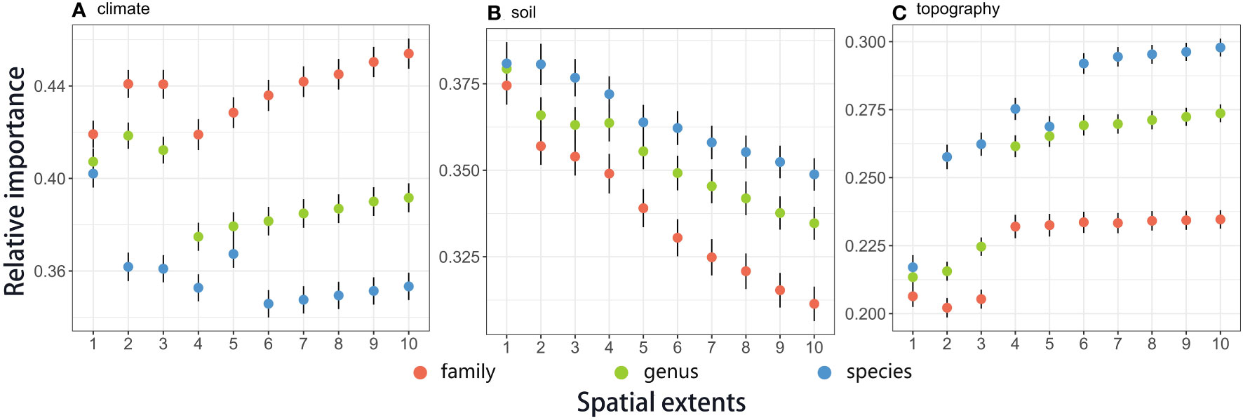
Figure 2 Relative importance of climate, soil, and topography variables on plant distributions across taxonomic scales (family, genus, and species) and spatial extents (1° × 1°, 2° × 2°, 3° × 3°, 4° × 4°, 5° × 5°, 6° × 6°, 7° × 7°, 8° × 8°, 9° × 9°, and 10° × 10°). Points and vertical lines showed the means and standard errors, respectively. The regressions were weighted by the inverse of the standard errors. Climate variables contain solar radiation and the three PC axes of temperature and precipitation. Soil variables contain the five PC axes of soil properties. Topographic variables include elevation, slope, and aspect. Trends in specific factors are shown in Supplementary Information Appendix S1: Table S1.2.

We found significant scale-dependence patterns of different environmental effects across spatial extents (1° × 1°, 2° × 2°, 3° × 3°, 4° × 4°, 5° × 5°, 6° × 6°, 7° × 7°, 8° × 8°, 9° × 9° and 10° × 10° at the regional scale) on plant (family, genus, and species) distributions (Figure 2 and Table 1). Overall, climate and topography increased their importance in determining plant distributions with larger spatial extents (Figures 2A, C), while soil showed the opposite trends (Figure 2B). Trends in topographical effects across spatial scales were relatively flatter than for climate and soil. Notably, 4° × 4° appeared to be a threshold for trends in climate and topography: clear rising trends for climate and flatter trends for topography could be found at extents larger than 4° × 4°.

Table 1

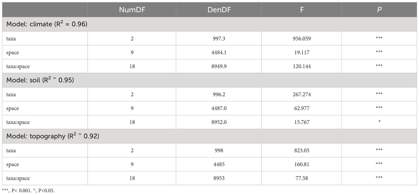
Table 1 Effects of spatial extents (i.e., 1° × 1°, 2° × 2°, 3° × 3°, 4° × 4°, 5° × 5°, 6° × 6°, 7° × 7°, 8° × 8°, 9° × 9° and 10° × 10°) and taxonomic scales (i.e., family, genus, and species levels) on the relative importance of the impact of environmental factors (categorized into three groups: climate, soil, and topography) on plant distributions.

Within each group of climate, soil, and topography, environmental factors showed differential importance with changing spatial extents (Figure 3). For example, despite the general decreasing tendency of soil variables, two of soil PCs (PC4 and PC8) showed diverse trends across spatial scales. For topographical variables, aspect and slope presented a similar growth tendency with spatial extent, while elevation showed much more variation among the studied plots (Diagrams 10–12 in Figure 3). With the exception of these, the trends in most specific factors were basically consistent with the general trend of climate, soil, or topography across spatial scales.

Figure 3

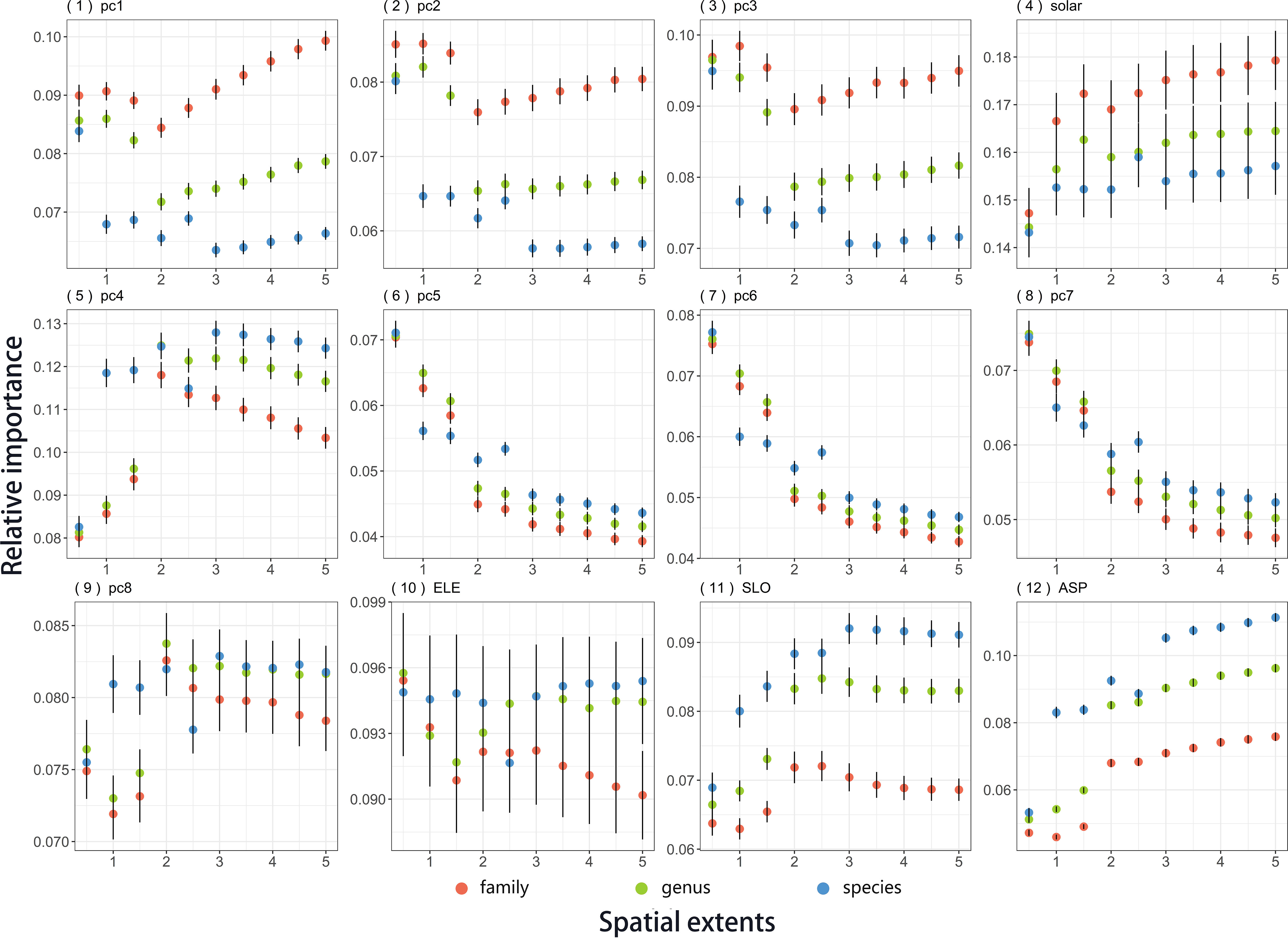
Figure 3 Relative importance of 12 environmental factors on plant distribution across taxonomic levels (family, genus, and species) and spatial extents (1° × 1°, 2° × 2°, 3° × 3°, 4° × 4°, 5° × 5°, 6° × 6°, 7° × 7°, 8° × 8°, 9° × 9° and 10° × 10°). Points and vertical lines show the means and two times of the standard error, respectively. Predicted lines were from the regressions of the relative importance of environmental variables against the area of regional plots, which were performed separately for each taxonomic level. The regressions were weighted by the inverse of the standard errors. Environmental variables were as follows: climate (PC1 to PC3, Solar), soil (PC4 to PC 8) and topography (ELE, SLO, ASPL). Abbreviations of environmental factors are defined in Table S1.2.

The relative importance of environmental variables on plant distributions significantly differed among the taxonomic scales (i.e., family, genus, and species) (Figures 2, 3; Tables 1, S1.2). Generally, climate had a larger influence on plant distributions at higher taxonomic levels than that at lower ones (i.e., family>genus>species. Figure 2A). However, for soil and topography, variables were more important at the species than genus levels, followed by the family level (Figures 2B, C).

For climate, most factors had less importance on plant distributions at the family level than at the species and genus levels (Diagrams 1–4 in Figure 3). On the contrary, edaphic factors had higher importance at finer taxonomic scales, with exceptions at particular spatial extents (e.g., PC5 and PC6 at 2° × 2° and 3° × 3°; Figure 2B and Diagrams 5–9 in Figure 3). Topography had a similar rank as soil (species> genus >family), in spite of a complex pattern in elevation where the ranking changed diversely at different spatial scales (Figure 2C, Diagrams 10–12 in Figure 3). The difference in the relative effects among the three taxonomic levels was finer in the soil variables than climate and topography (Figure 2 and Diagrams 5–9 in Figure 3).

The relative importance of environmental factors showed varying spatial-dependence trends at different taxonomic levels (Figures 2, 3). For example, plant species did not show apparent increasing trends in the relative importance of climate effects such as family and genus (Diagram 1 in Figure 2). The interactive effects between spatial extent and taxonomic scale on environmental importance were statistically significant (Table 1 and Supplementary Information Appendix S1: Table S1.5), indicating the interplay of spatial and taxonomic scales on the influence of the environment on plant distributions. Some factors such as elevation and solar radiation showed contrary trends with increasing spatial extents at the family and genus levels (Diagrams 4 and 10 in Figure 3). Variations in the relative importance of soil variables among the family, genus, and species levels were comparatively smaller when considering the specific edaphic variables (Figure 2B and Diagrams 5–8 in Figure 3).

Discussion

Our study found significant evidence for both the spatial and taxonomic scale-dependence of environmental effects on plant distributions (Table 1). Climate variables showed greater importance at larger spatial (larger than 4° × 4°) and higher taxonomic scales (Table 1 and Figures 2A, 3), while soil variables exhibited opposite trends for both spatial and taxonomic scales (Table 1 and Figures 2B, 3). Topography indicated a relatively slow increase with spatial scale, with a larger impact on plant distributions at the species level than at the genus and family levels (Table 1 and Figures 2C, 3). These findings emphasize the scale-dependence of the relative environmental effects that shape plant distributions, suggesting a multi-scale insight into studying plant–environment relationships. Here we discuss our main findings and the potential mechanisms below.

Scale dependence of climate effects

Climatic variables had a larger impact on plant distributions when the spatial and taxonomic scales increased at spatial extents larger than 4° × 4°. The results overall support our hypotheses (H1) relating to the spatial and taxonomic scale-dependence patterns of climate effects on plant distributions within limited scales. These results are congruent with past descriptions and analyses of the vegetation of the world (as far back as Von Humboldt, 1805). High spatial variation in climate conditions at large spatial scales may possibly explain the spatial scale-dependence of climatic effects on plant distributions. However, stochasticity appeared at fine scales (<4° × 4°), where the trends in climate effect with spatial scale varied significantly among different taxonomic levels. These may due to the variety of local processes (e.g., stochastic processes) at finer spatial scales. Thus, it is more reliable to use climate variables for predicting plant distribution patterns at a relatively broad spatial scale, where climatic constraints such as temperature extremes and light intensity restrict plant radiation across the globe.

Plants have evolved traits to adapt to climate change and extreme climate (e.g., episodic freezing) or have dispersed to more suitable areas (Zanne et al., 2014). The relative importance of climatic effects among different taxonomic levels shows that the response of plants to climate may be more distinct between families than within families (e.g., among species), indicating that the climate-related traits of plants are the consequence of long-term adaptive evolution (Zanne et al., 2014).

Scale dependence of soil effects

Soil was more important at finer spatial scales and at lower taxonomic levels (i.e., species>genus>family), which aligns well with our hypothesis (H2). The effects of soil on plant distributions diminished at large spatial extents with greater soil heterogeneity (Figure 2B). Soil heterogeneity at fine spatial scale may cause variation in the strength of ecological processes that shape local plant distributions and coexistence, such as the root absorption of nutrients, microbe shifts, and mycorrhizal symbiosis (Smith & Read, 1997; Callaway, 2007; Wang et al., 2019).

Soil effects were stronger at relatively lower taxonomic scales (Figure 2B), suggesting that fine-scale processes related to soil (e.g., plant–soil feedback) are more likely to vary among species than families. This indicated that these processes may be driven by recent events and thus may be more dynamic. Despite the general decreasing trends in soil effects with spatial and taxonomic scales, specific factors within the category showed different patterns (Figures 2B, 3). For example, the relative importance of PC4 and PC8 (mainly representing soil texture and gravel, respectively) increased with spatial extents. This implies that internal processes related to soil niche are complex and varied.

Scale dependence of topography effects

The topographical effects on plant distribution were relatively intricate and unpredictable across spatial scales (Figures 2C, 3). Topographical factors affect plant distributions by causing changes in other ecological conditions (Irl et al., 2015; Slaton, 2015; Muscarella et al., 2020), such as the microclimate and edatope of plant habitats along an elevational gradient, which is nonlinear and difficult to predict. Nevertheless, their influences are perhaps strongly related to the presence of montane species with a limited range in mountainous areas. Thus, topographical effects should not be continually increased at large scales beyond the geographical range of mountains. This was confirmed in our analysis whereby the trends in topographical effects that increased with spatial scale flattened at spatial extents larger than 4° × 4° (with the exception of 6° × 6° for species; Figure 2C).

The influence of topography on plant distributions also emanates from the unique evolutionary histories of montane ecosystems (Muellner-Riehl et al., 2019). Topographical factors showed more influence at the species level than at the genus and family levels (Figure 2C). This result supports our hypothesis of the taxonomic scale-dependence of topographical effects (H3), revealing the impact of evolutionary history on montane floras. Topography probably had a stronger effect on species than on families because montane floras tend to be related to nearby lowland floras. On the contrary, most of the variation in plant distributions caused by topographical changes has occurred recently in evolutionary history (Kelly & Goulden, 2008).

Limitations of study scale dependence

Generally, climate variables’ relative importance is larger than topography and soil (Figure 2), which is similar to results of our former study on environmental effects on global plant distributions (Huang et al., 2021). However, the detection of environmental effects depends on the methods we use. Additional analyses of other measurements (e.g., MaxEnt model) also show similar trends in relative environmental effects changing with spatial and taxonomic scales, though different in importance value to some degrees (Supplementary Information Appendix S3).

Nevertheless, it is still difficult to know how multi-scale processes interact with each other that shape the scale-dependence patterns in our study using large-scale occurrence data. For example, global and regional changes in biological diversity are the origins and consequences of fine-scale phenomena (Levin, 1992) or assemblage-level processes (e.g., biotic interaction and dispersal). The interplay of multi-scale and cross-scale processes is actually comprehensive and poorly understood, and further studies integrating community ecology, macroecology, and macroevolution are needed.

Conclusion

Our study reveals the scale-dependence of environmental effects on plant distributions, indicating various ecological processes underlying plant distribution patterns across spatial and taxonomic scales. However, the internal mechanistic processes require further exploration. Overall, we highlighted the importance of scales in disentangling plant–environment relationships and other ecological studies. It is important to integrate the diverse ecological patterns driven by multi-scale processes from the population and community to macroecological perspectives, to better understand natural systems across time and space.

Data availability statement

The datasets presented in this study can be found in online repositories. The names of the repository/repositories and accession number(s) can be found below: https://doi.org/10.6084/m9.figshare.22678138.v1.

Author contributions

EH and SY developed the research question. EH conducted data analyses and wrote the first draft of the manuscript. EH, YC and SY contributed substantially to the discussion, writing and revisions of the manuscript. All authors contributed to the article and approved the submitted version.

Funding

The author(s) declare financial support was received for the research, authorship, and/or publication of this article. This research was funded by National Natural Science Foundation of China (Grant 31830010, 31770513) and the National Key Research and Development Program of China (Project No. 2017YFA0605100).

Acknowledgments

We are grateful to many scientists for their thorough surveys of flora diversity and collection of environmental factors.

Conflict of interest

The authors declare that the research was conducted in the absence of any commercial or financial relationships that could be construed as a potential conflict of interest.

Publisher’s note

All claims expressed in this article are solely those of the authors and do not necessarily represent those of their affiliated organizations, or those of the publisher, the editors and the reviewers. Any product that may be evaluated in this article, or claim that may be made by its manufacturer, is not guaranteed or endorsed by the publisher.

Supplementary material

The Supplementary Material for this article can be found online at: https://www.frontiersin.org/articles/10.3389/fevo.2023.1233936/full#supplementary-material

Footnotes

1. ^ The Plant List (2013). Version 1.1. Published online; http://www.theplantlist.org/ (accessed 1st January, 2019).
2. ^ Data obtained from the “Global Solar Atlas 2.0, a free, web-based application developed and operated by the company Solargis s.r.o. on behalf of the World Bank Group, utilizing Solargis data, with funding provided by the Energy Sector Management Assistance Program (ESMAP). For additional information: https://globalsolaratlas.info.

References

Barbet-Massin M., Jiguet F., Albert C. H., Thuiller W. (2012). Selecting pseudo-absences for species distribution models: How, where and how many? Methods Ecol. Evol. 3 (2), 327–338. doi: 10.1111/j.2041-210X.2011.00172.x

CrossRef Full Text | Google Scholar

Barry R. G. (2008). Mountain Weather and Climate (Cambridge, UK: Cambridge University Press).

Google Scholar

Bartoń K. (2013) MuMIn: Multi-Model Inference. R package version 1.43.17. Available at: https://CRAN.R-project.org/package=MuMIn.

Google Scholar

Beauregard F., de Blois S. (2014). Beyond a climate-centric view of plant distribution: edaphic variables add value to distribution models. PloS One 9 (3), e92642. doi: 10.1371/journal.pone.0092642

PubMed Abstract | CrossRef Full Text | Google Scholar

Breiman L. (2001). Random forests. Mach. Learn. 45 (1), 5–32. doi: 10.1023/A:1010933404324

CrossRef Full Text | Google Scholar

Callaway R. ,. M. (2007). Positive interactions and interdependence in plant communities (New York: Springer). doi: 10.1007/978-1-4020-6224-7

CrossRef Full Text | Google Scholar

Chave J., Bascompte J. (2013). The problem of pattern and scale in ecology, what have we learned in 20 years? Ecol. Lett. 16, 4–16.

PubMed Abstract | Google Scholar

Cox C. B., Moore P. D. (1985). Biogeography, an ecological and evolutionary approach (Blackwell Scientific: Oxford).

Google Scholar

Crawley M. J., Harral J. E. (2001). Scale dependence in plant biodiversity. Science 291 (5505), 864. doi: 10.1126/science.291.5505.864

PubMed Abstract | CrossRef Full Text | Google Scholar

Cutler D. R., Edwards T. C. Jr., Beard K. H., Cutler A., Hess K. T., Gibson J., et al. (2007). Random forests for classification in ecology. Ecology 88 (11), 2783–2792. doi: 10.1890/07-0539.1

PubMed Abstract | CrossRef Full Text | Google Scholar

Davies K. F., Chesson P., Harrison S., Inouye B. D., Melbourne B. A., Rice K. J. (2005). Spatial heterogeneity explains the scale dependence of the native-exotic diversity relationship. Ecology 86 (6), 1602–1610. doi: 10.1890/04-1196

CrossRef Full Text | Google Scholar

Elith J., Leathwick J. R. (2009). Species distribution models, ecological explanation and prediction across space and time. Annu. Rev. Ecol. Evol. Syst. 40 (1), 677–697. doi: 10.1146/annurev.ecolsys.110308.120159

CrossRef Full Text | Google Scholar

Evans J. S., Cushman S. A. (2009). Gradient modeling of conifer species using random forests. Landscape Ecol. 24, 673–683. doi: 10.1007/s10980-009-9341-0

CrossRef Full Text | Google Scholar

Fischer G., Nachtergaele F., Prieler S., van Velthuizen H. T., Verelst L., Wiberg D. (2008). Global Agro-ecological Zones Assessment for Agriculture (GAEZ 2008) (Rome, Italy: IIASA, Laxenburg, Austria and FAO).

Google Scholar

Genuer R., Poggi J.-M., Tuleau-Malot C. (2010). Variable selection using random forests. Pattern Recognit. Lett. 31 (14), 2225–2236. doi: 10.1016/j.patrec.2010.03.014

CrossRef Full Text | Google Scholar

Graham C. H., Storch D., Machac A. (2018). Phylogenetic scale in ecology and evolution. Global Ecol. Biogeogr. 27 (2), 175–187. doi: 10.1111/geb.12686

CrossRef Full Text | Google Scholar

Guisan A., Thuiller W. (2005). Predicting species distribution, offering more than simple habitat models. Ecol. Lett. 8 (9), 993–1009. doi: 10.1111/j.1461-0248.2005.00792.x

PubMed Abstract | CrossRef Full Text | Google Scholar

Hong H., Xiaoling G., Hua Y. (2016). “Variable selection using Mean Decrease Accuracy and Mean Decrease Gini based on Random Forest,” in 2016 7th IEEE International Conference on Software Engineering and Service Science (ICSESS), Beijing. pp. 219–224. doi: 10.1109/ICSESS.2016.7883053

CrossRef Full Text | Google Scholar

Huang E., Chen Y., Fang M., Zheng Y., Yu S. (2021). Environmental drivers of plant distributions at global and regional scales. Global Ecol. Biogeogr. 30, 697–709. doi: 10.1111/geb.13251

CrossRef Full Text | Google Scholar

Hutchinson G. E. (1957). Concluding remarks. Cold Spring Harbor Symp. 22, 415–427. doi: 10.1101/SQB.1957.022.01.039

CrossRef Full Text | Google Scholar

Irl S. D. H., Harter D. E. V., Steinbauer M. J., Gallego Puyol D., Fernández-Palacios J. M., Jentsch A., et al. (2015). Climate vs. topography-spatial patterns of plant species diversity and endemism on a high-elevation island. J. Ecol. 103 (6), 1621–1633. doi: 10.1111/1365-2745.12463

CrossRef Full Text | Google Scholar

Jamir E., Kangabam R. D., Borah K., Tamuly A., Deka Boruah H. P., Silla Y. (2019). “Role of Soil Microbiome and Enzyme Activities in Plant Growth Nutrition and Ecological Restoration of Soil Health,” in Microbes and Enzymes in Soil Health and Bioremediation. Eds. Kumar A., Sharma S. (Singapore: Springer Singapore), 99–132.

Google Scholar

Kelly A. E., Goulden M. L. (2008). Rapid shifts in plant distribution with recent climate change. Proc. Natl. Acad. Sci. 105 (33), 11823. doi: 10.1073/pnas.0802891105

CrossRef Full Text | Google Scholar

Levin S. A. (1992). The problem of pattern and scale in ecology, the robert H. MacArthur award lecture. Ecology 73 (6), 1943–1967.

Google Scholar

Levin D. A. (2019). Plant speciation in the age of climate change. Ann. Bot. 124 (5), 769–775. doi: 10.1093/aob/mcz108

PubMed Abstract | CrossRef Full Text | Google Scholar

Liaw A., Wiener M. (2002). Classification and regression by randomForest. R. News 2 (3), 18–22.

Google Scholar

Lin G., Stralberg D., Gong G., Huang Z., Ye W., Wu L. (2013). Separating the effects of environment and space on tree species distribution, from population to community. PloS One 8 (2), e56171. doi: 10.1371/journal.pone.0056171

PubMed Abstract | CrossRef Full Text | Google Scholar

Lomolino M. V. (2001). Elevation gradients of species-density: historical and prospective views. Global Ecol. Biogeogr. 10 (1), 3–13. doi: 10.1046/j.1466-822x.2001.00229.x

CrossRef Full Text | Google Scholar

Marage D., Gégout J.-C. (2009). Importance of soil nutrients in the distribution of forest communities on a large geographical scale. Global Ecol. Biogeogr. 18, 88–97. doi: 10.1111/j.1466-8238.2008.00428.x

CrossRef Full Text | Google Scholar

Martinez-Almoyna C., Piton G., Abdulhak S., Boulangeat L., Choler P., Delahaye T., et al. (2020). Climate, soil resources and microbial activity shape the distributions of mountain plants based on their functional traits. Ecography 43, 1550–1559. doi: 10.1111/ecog.05269

CrossRef Full Text | Google Scholar

Muellner-Riehl A. N., Schnitzler J., Kissling W. D., Mosbrugger V., Rijsdijk K. F., Seijmonsbergen A. C., et al. (2019). Origins of global mountain plant biodiversity: Testing the ‘mountain-geobiodiversity hypothesis’. J. Biogeogr. 46, 2826–2838. doi: 10.1111/jbi.13715

CrossRef Full Text | Google Scholar

Münzbergová Z. (2004). Effect of spatial scale on factors limiting species distributions in dry grassland fragments. J. Ecol. 92, 854–867. doi: 10.1111/j.0022-0477.2004.00919.x

CrossRef Full Text | Google Scholar

Muscarella R., Kolyaie S., Morton D. C., Zimmerman J. K., Uriarte M. (2020). Effects of topography on tropical forest structure depend on climate context. J. Ecol. 108, 145–159. doi: 10.1111/1365-2745.13261

CrossRef Full Text | Google Scholar

Nakagawa S., Schielzeth H. (2013). A general and simple method for obtaining R² from generalized linear mixed-effects models. Methods Ecol. Evol. 4, 133–142. doi: 10.1111/j.2041-210x.2012.00261.x

CrossRef Full Text | Google Scholar

Ni M., Vellend M. (2024). Soil properties constrain predicted poleward migration of plants under climate change. New Phytol. 241, 131–141. doi: 10.1111/nph.19164

PubMed Abstract | CrossRef Full Text | Google Scholar

Olson D. M., Dinerstein E., Wikramanayake E. D., Burgess N. D., Powell G. V. N., Underwood E. C., et al. (2001). Terrestrial ecoregions of the world: a new map of life on Earth. Bioscience 51 (11), 933–938. doi: 10.1641/0006-3568(2001)051[0933:TEOTWA]2.0.CO;2

CrossRef Full Text | Google Scholar

Perlwitz J., Knutson T., Kossin J. P., LeGrande A. N. (2017). Large-scale circulation and climate variability. In, Climate Science Special Report, Fourth National Climate Assessment, Volume I. Eds. Wuebbles D. J., Fahey D. W., Hibbard K. A., Dokken D. J., Stewart B. C., Maycock T. K. (Washington, DC, USA: U.S. Global Change Research Program), 161–184.

Google Scholar

Pinheiro J., Bates D., DebRoy S., Sarkar D., R Core Team (2021) nlme: linear and nonlinear mixed effects models. Available at: https://CRAN.R-project.org/package=nlme.

Google Scholar

Queenborough S. A., Burslem D. F. R. P., Garwood N. C., Valencia R. (2009). Taxonomic scale-dependence of habitat niche partitioning and biotic neighborhood on survival of tropical tree seedlings. Proc. Biol. Sci. 276 (1676), 4197–4205. doi: 10.1098/rspb.2009.0921

PubMed Abstract | CrossRef Full Text | Google Scholar

R Core Team. (2023). _R: A Language and Environment for Statistical Computing_. (Vienna, Austria: R Foundation for Statistical Computing). Available at: https://www.R-project.org/.

Google Scholar

Schweiger A. H., Beierkuhnlein C. (2016). Scale dependence of temperature as an abiotic driver of species’ distributions. Global Ecol. Biogeogr. 25 (8), 1013–1021. doi: 10.1111/geb.12463

CrossRef Full Text | Google Scholar

Shangguan W., Dai Y., Duan Q., Liu B., Yuan H. (2014). A global soil data set for earth system modeling. J. Adv. Modeling. Earth Syst. 6 (1), 249–263. doi: 10.1002/2013ms000293

CrossRef Full Text | Google Scholar

Siefert A., Ravenscroft C., Althoff D., Alvarez-Yépiz J. C., Carter B. E., Glennon K. L., et al. (2012). Scale dependence of vegetation-environment relationships, a meta-analysis of multivariate data. J. Vegetation. Sci. 23, 942–951. doi: 10.1111/j.1654-1103.2012.01401.x

CrossRef Full Text | Google Scholar

Slaton M. R. (2015). The roles of disturbance, topography and climate in determining the leading and rear edges of population range limits. J. Biogeogr. 42, 255–266. doi: 10.1111/jbi.12406

CrossRef Full Text | Google Scholar

Smith S. E., Read D. J. (1997). Mycorrhizal symbiosis (San Diego: Academic press).

Google Scholar

Vargas O. M., Goldston B., Grossenbacher D. L., Kay K. M. (2020). Patterns of speciation are similar across mountainous and lowland regions for a Neotropical plant radiation (Costaceae: Costus). Evolution 74, 2644–2661. doi: 10.1111/evo.14108

PubMed Abstract | CrossRef Full Text | Google Scholar

Viana D. S., Chase J. M. (2019). Spatial scale modulates the inference of metacommunity assembly processes. Ecology 100 (2), e02576. doi: 10.1002/ecy.2576

PubMed Abstract | CrossRef Full Text | Google Scholar

Von Humboldt A. (1805). Voyage aux regions equinoxiales du Nouveau Continent, fait en 1799, 1800, 1801, 1802, 1802, 1803 et 1804 par Al. de Humboldt et A. Bonpland. Paris: Redige par Alexandre de Humboldt (transl. to German).

Google Scholar

Wang C., McCormack M. L., Guo D., Li J. (2019). Global meta-analysis reveals different patterns of root tip adjustments by angiosperm and gymnosperm trees in response to environmental gradients. J. Biogeogr. 46 (1), 123–133. doi: 10.1111/jbi.13472

CrossRef Full Text | Google Scholar

Weil R., Brady N. C. (2017). The Nature and Properties of Soils. 15th edition (New York: Pearson).

Google Scholar

Whittaker R. H. (1975). Communities And Ecosystems. 2nd edition (New York: Macmillan Publishing Company).

Google Scholar

Wiens J. A. (1989). Spatial scaling in ecology. Funct. Ecol. 3, 385–397. doi: 10.2307/2389612

CrossRef Full Text | Google Scholar

Woodward F. I., Lomas M. R., Kelly C. K. (2004). Global climate and the distribution of plant biomes. Philos. Trans. R. Soc. London. Ser. B Biol. Sci. 359 (1450), 1465–1476.S. doi: 10.1098/rstb.2004.1525

CrossRef Full Text | Google Scholar

Woodward F. I., Williams B. G. (1987). Climate and plant distribution at global and local scales. Vegetatio 69, 189. doi: 10.1007/BF00038700

CrossRef Full Text | Google Scholar

Yackulic C. B., Ginsberg J. R. (2016). The scaling of geographic ranges, implications for species distribution models. Landscape Ecol. 31 (6), 1195–1208. doi: 10.1007/s10980-015-0333-y

CrossRef Full Text | Google Scholar

Yeh C.-F., Soininen J., Teittinen A., Wang J. (2019). Elevational patterns and hierarchical determinants of biodiversity across microbial taxonomic scales. Mol. Ecol. 28 (1), 86–99. doi: 10.1111/mec.14935

PubMed Abstract | CrossRef Full Text | Google Scholar

Zanne A. E., Tank D. C., Cornwell W. K., Eastman J. M., Smith S. A., FitzJohn R. G., et al. (2014). Three keys to the radiation of angiosperms into freezing environments. Nature 506, 89–92. doi: 10.1038/nature12872

PubMed Abstract | CrossRef Full Text | Google Scholar

Zizka A., Silvestro D., Andermann T., Azevedo J., Duarte Ritter C., Edler D., et al. (2019). CoordinateCleaner: Standardized cleaning of occurrence records from biological collection databases. Methods Ecol. Evol. 10, 744–751. doi: 10.1111/2041-210X.13152

CrossRef Full Text | Google Scholar