Exposure of marine megafauna to cumulative anthropogenic threats in north-west Australia

As the use of coastal and offshore environments expands, there is a need to better understand the exposure of marine megafauna to anthropogenic activities that potentially threaten their populations. Individual satellite telemetry studies are often hampered by small sample sizes, providing limited information on spatiotemporal distributions of migratory animals and their relationships to anthropogenic threats. We addressed this issue by synthesising satellite tracking data from 484 individuals of three taxonomic groups and six species; three marine turtle, two whale and one shark. The spatial overlap between taxa distributions and multiple anthropogenic activities was assessed as a proxy for the cumulative exposure of these taxa to anthropogenic threats (coastal modification, vessel strike, underwater noise, oil spill, bycatch, entanglement, and artificial light) across an area totalling 2,205,740 km² off north-western Australia. Core exposure areas (top 50% of the distribution) encompassed ecologically important sites for all taxa, such as the Ningaloo and Pilbara regions, migratory routes for whales and sharks in offshore waters beyond Ningaloo Reef, and marine turtle nesting beaches at Barrow Island and Cape Lambert. Although areas of high exposure represented <14% of taxa distributions, we showed that no taxa occurred in the absence of threats and that even areas with existing spatial protections are experiencing high levels of exposure. Importantly, we developed a robust approach for documenting the potential exposure of marine species to a range of human activities at appropriate spatial scales to inform conservation management.

1 Introduction

Loss of biodiversity is a global crisis driven by a myriad of anthropogenic threats (Barnosky et al., 2011). In marine environments, many species are exposed to an increasing number and intensity of threatening processes as human use of these environments expands (e.g., Halpern et al., 2008; Barnosky et al., 2011; Maxwell et al., 2013; Bowler et al., 2020). Threat mapping has emerged as a powerful tool for management strategies that seek to mitigate these threats and has allowed for conservation management actions to be prioritised for areas and species at most risk (e.g., Maxwell et al., 2013; Tulloch et al., 2015; Ostwald et al., 2021).

Although there is often a good theoretical understanding of the range of threats potentially acting on the marine environment globally (Halpern et al., 2008; Bowler et al., 2020), data on species distributions at scales appropriate to undertake quantitative assessments of spatial overlap to inform management are often limited. Satellite telemetry provides these data for many species, however, sample sizes within individual studies are usually restrained by logistics and cost. The synthesis of data across multiple projects offers an approach that overcomes these issues and can produce sample sizes at spatial and temporal scales sufficient to be representative of sub-populations, populations or ecosystems (Sequeira et al., 2019; Hindell et al., 2020; Ferreira et al., 2021; Fossette et al., 2021a). Telemetry data can then be combined with threat mapping to provide a powerful means of documenting the potential exposure of species to a range of human activities, with the ultimate goal of enabling more targeted conservation management.

Increasing human population’s demands for resources, and technological advances have led to an expansion of coastal and offshore activities (e.g., seismic surveys, drilling, shipping, fishing) and associated infrastructure (oil and gas platforms, ports, aquaculture farms) worldwide, which can have a series of direct and indirect impacts on the marine ecosystem. These impacts can include displacement, increased species injury and mortality rates, reduced fitness and the modification of seafloor and other habitats, (Halpern et al., 2008; Kamrowski et al., 2012; Kark et al., 2015; Falchi et al., 2016). For example, bycatch from fishing is a major cause of mortality for large marine fauna such as elasmobranchs, cetaceans and marine turtles (Roberson et al., 2022), with high overlap occurring between their preferred habitat and areas with high levels of fishing pressure (Žydelis et al., 2013; Queiroz et al., 2016; Queiroz et al., 2019). The exposure to both chronic and acute industrial underwater noise (e.g. recreational boating, shipping, seismic surveys, drilling, dredging and pile driving activities) is also considered a major threat to cetaceans (Avila et al., 2018; Hart et al., 2018; Hückstädt et al., 2020). These threatening processes can lead to the disruption of behaviours critical to species survival (e.g., feeding and reproduction), localised displacement from important areas, stress and potential hearing damage and mortality (McCauley et al., 2000; Gordon et al., 2003; Kamrowski et al., 2012; Hawkins et al., 2015; Nelms et al., 2016; Wilson et al., 2018; Elliott et al., 2019; Wilson et al., 2019; Dunlop et al., 2021). Consequently, there is an urgent need for a better understanding of the exposure of marine megafauna populations to anthropogenic threats to allow more holistic risk assessment and guide management actions.

Here, we compiled satellite telemetry data from multiple studies to determine the spatial distributions of six species of threatened and migratory marine megafauna across three taxonomic groups (marine turtles, whales and sharks) off the North-West Marine and North Marine regions in Australia. We combined taxa distributions with spatial data from multiple coastal and offshore human activities that occur in this region, used their spatial overlap as a proxy for quantifying exposure to anthropogenic threats and identified key areas within taxa distributions where high exposure to cumulative threats exist. This output is required to support sustainable use and conservation management in a region with diverse marine habitats and communities that are also economically significant areas for coastal and offshore industry, commercial fisheries, and the extraction, processing and shipping of resources (e.g. oil, gas and, iron ore) to overseas ports (Fossette et al., 2021b).

2 Methods

2.1 Study site

We compiled satellite telemetry data from marine megafauna satellite tagged in the North-West Marine Region of the Australian Exclusive Economic Zone (EEZ) (henceforth referred to as ‘north-west Australia’) (Figure 1, Supplementary Table S2). The North Marine Region was also included in our analyses as many individuals tagged in north-west Australia moved there (Figure 1). These two regions encompass an area totalling 2,205,740 km² and covering 38% of the Australian EEZ.

Figure 1

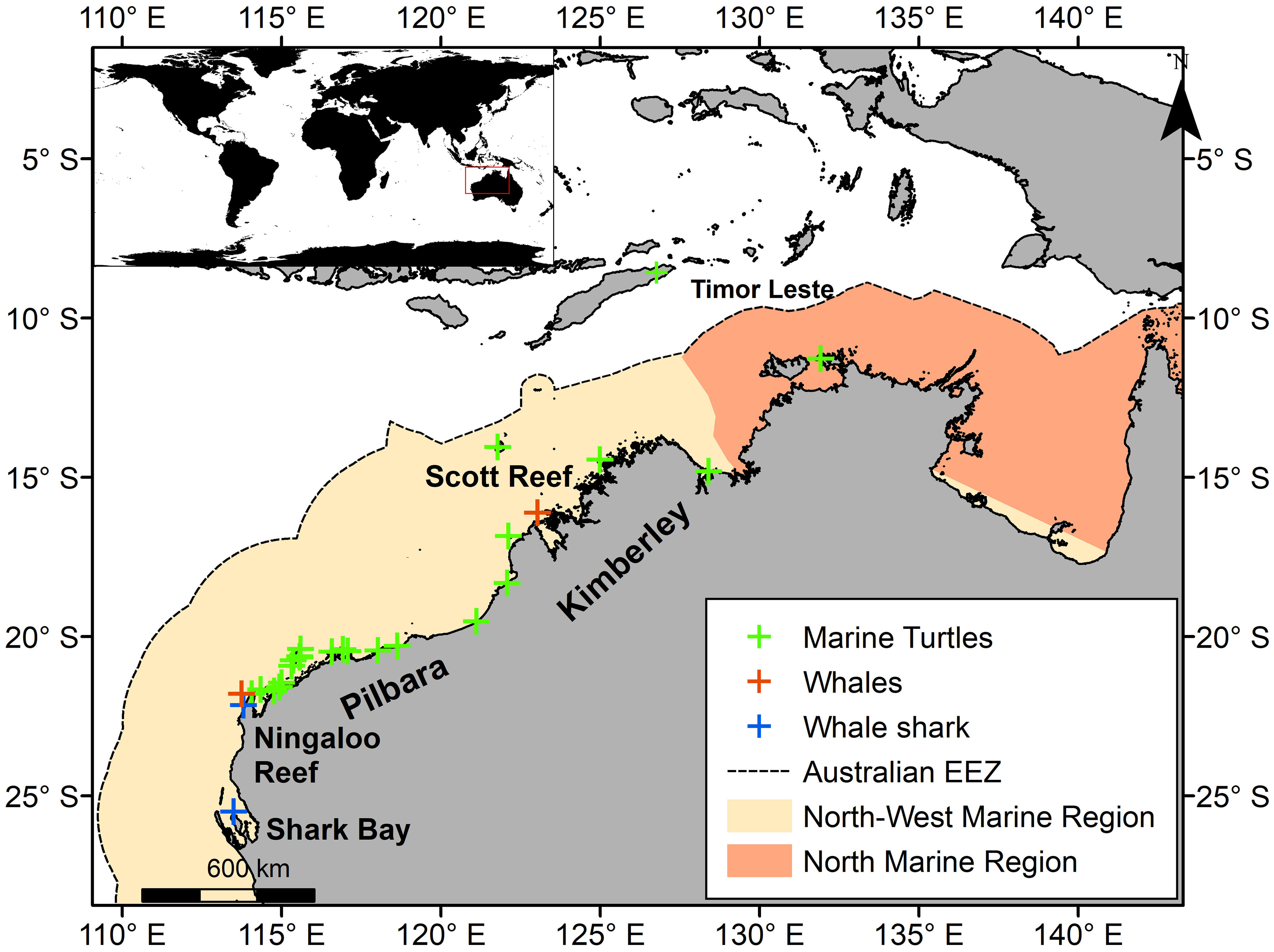
Figure 1 Study area with satellite tag deployment locations for marine turtles, whales, and whale sharks in the North-West and North Marine regions. Inset (top left) shows location of study region. Tagging locations for pygmy blue whales tagged at Perth Canyon (32°S, 114°E 58') and Bonney Coast (37°S, ~140°E) (Supplementary Table S2) are outside the study area and satellite tracking data for these species were trimmed to start at the southern extent of the study area (27°S).

2.2 Marine megafauna data

2.2.1 Satellite tracking data compilation

We compiled existing satellite tracking data for threatened marine megafauna (Supplementary Table S2), including 96 green (Chelonia mydas), 42 hawksbill (Eretmochelys imbricata), and 251 flatback turtles (Natator depressus); 19 humpback (Megaptera novaeangliae), and 20 pygmy blue whales (Balaenoptera musculus brevicauda); and 56 whale sharks (Rhincodon typus). These datasets comprised most of the existing satellite tracking data from threatened marine megafauna in the region. Although some data exist for other species not included here such as dugongs Dugong dugon (Kennet and Kitchens, 2009; Bayliss and Hutton, 2017), frigate birds (Mott et al., 2017) and loggerhead turtles Caretta caretta (Tucker, unpublished data), these had low sample size and/or low spatial coverage over the study region and/or were unavailable?.

Satellite transmitters were deployed on nesting female turtles at major rookeries in Western Australia and one hawksbill rookery in Timor Leste (Figure 1). Between 2000 and 2018 tags were deployed during the breeding season (October – January and July), providing data on use of inter-nesting habitats and migration to foraging grounds of adult female turtles (Supplementary Table S2) (Pendoley, 2005; Waayers et al., 2011; Whittock et al., 2016; Thums et al., 2017; Thums et al., 2018; Ferreira et al., 2021; Fossette et al., 2021a).

Humpback whales were tagged on two different occasions. Seven adult female humpback whales with dependent calves were tagged in coastal waters of the Kimberley region, Western Australia, during their southbound migration to feeding grounds from the tropics to Antarctic waters in August and September 2009 (Double et al., 2009; Double et al., 2010; Bestley et al., 2019). Humpback whales of both sexes were also tagged off Ningaloo Reef, Western Australia, on their northward migration to breeding grounds in north-west Australia in July 2011 (n = 13) (Figure 1; Supplementary Table S2).

Pygmy blue whales were tagged off their feeding grounds in the Perth Canyon, Western Australia, Northwest Cape, Western Australia and the Bonney Upwelling region, South Australia prior to their migration to wintering grounds in Indonesia. The Perth Canyon dataset included nine individuals (3 males, 3 females, 3 unknown sex) tagged in March – April 2009 and 2011 (Double et al., 2014), and four of unknown sex tagged in April 2021 (Thums et al., 2022). We included one animal tagged in March 2015 in the Bonney Upwelling region that migrated into the study region (Möller et al., 2020). The dataset for Northwest Cape (the northern tip of Ningaloo Reef) included six whales tagged in May – June 2019 and 2020 (Thums et al., 2022) (Figure 1, Supplementary Table S2).

Whale sharks (n = 56) were tagged during the seasonal aggregation at Ningaloo Reef and Shark Bay, Western Australia, between 2005 – 2007 and 2010 – 2018 (Wilson et al., 2006; Sleeman et al., 2010; Norman et al., 2016; Reynolds et al., 2017) (Figure 1, Supplementary Table S2).

We combined megafauna species data by the broad taxonomic groupings of whales, marine turtles, and sharks for subsequent analysis. This was done to aid interpretation and justified based on similarity in the pressures they encounter (Commonwealth of Australia, 2017), and the broad habitats (coastal versus offshore) used within most of their distribution across the study area (Pendoley, 2005; Waayers et al., 2011; Pendoley et al., 2014; Whittock et al., 2014; Whittock et al., 2016; Thums et al., 2017; Thums et al., 2018; Waayers et al., 2019; Ferreira et al., 2021; Fossette et al., 2021a). For example, although each of the turtles species use different habitats while foraging (seagrass for green turtles; Esteban et al., 2020, reef for hawksbill turtles; Whiting, 2000; Gaos et al., 2012, and soft bottom habitats for flatback turtles; Zangerl et al., 1988; Limpus and Fien, 2009), they are all benthic foragers and during foraging and migration they predominantly remain in coastal habitats (Pendoley et al., 2014; Ferreira et al., 2021; Fossette et al., 2021a). Although flatback turtles may use deeper habitats for foraging (water depths < 100 m deep; Thums et al., 2017) than the other two turtle species (median water depth of 14.5 m for hawksbills and 9 m for greens; Ferreira et al., 2021; Fossette et al., 2021a), all species remain well within continental shelf waters. Humpback whales are considered coastal in the region, however, they use more offshore waters, including off-shelf habitats during their southern migration (Bestley et al., 2019). This has overlap with pygmy blue whales that use offshore habitats, largely off the shelf in this region (Double et al., 2014; Thums et al., 2022).

The water depth associated with taxa distributions was calculated by overlaying spatial polygons of the distribution with bathymetry data obtained from the General Bathymetry Chart of the Oceans Gebco15 database with a 30 arc-second resolution grid (http://www.gebco.net) and extracting depth of water column.

2.2.2 Satellite tracking data processing

For datasets not previously analysed (346 out of 484), we applied a Bayesian switching state-space model (SSM) (Jonsen et al., 2003; Jonsen et al., 2005; Jonsen et al., 2019) to the raw satellite tracking data using the R (R Core Team, 2022) package bsam (Jonsen et al., 2017) for marine turtles, and the package foieGras (Jonsen, 2020) for whales and whale sharks. For datasets previously analysed (and published; 138 out of 484) using these same methods, we used the SSM output from those analyses, rather than refitting the SSM. Note that the main authors of this current paper (L Ferreira, M Thums and S Fossette), were authors on the previous publications (Ferreira et al., 2021; Fossette et al., 2021a) and so broad consistency in SSM analyses is confirmed. Both modelling methods (bsam and foieGras) account for location error and autocorrelation and predict true locations at a time step specified by the user. We selected a unique time step for each individual track based on the average number of actual locations received by the tags per day. Tracking data with gaps > 5 days were split and each portion of data analysed separately. For turtles, resident or transient movement states were assigned to each location of the track using the output from the SSM fitted with the bsam package. State space models using the package bsam for turtles were applied with a Bayesian switching first difference correlated random walk structure (DCRWS). To fit the model, we used a burn-in period of 120,000 samples, of which 80,000 were sampled from the posterior distribution, and every 80^th of the remaining samples were retained. Residency behaviour was further classified into residency associated with inter-nesting periods (period between laying clutches of eggs and before migrating to foraging grounds) or foraging as described in Thums et al. (2018) and Ferreira et al. (2021). Each of these behavioural modes (inter-nesting, migration and foraging) were analysed separately.

The foieGras package (now named aniMotum; Jonsen et al., 2023) provides an estimate of continuous movement persistence for each location along the track, where a low value implies residency behaviour, and a high value signifies transient movement. This method is useful when discrete behavioural states are unknown or less predictable (Breed et al., 2012; Jonsen et al., 2019) and for this reason, we used it to analyse the nomadic and large scale (100s km), migratory movements of whales and sharks. State space models using the package foieGras were applied with a correlated random walk structure and a maximum travel speed of 2.8 m/s for whales (Noad and Cato, 2007; Thums et al., 2022), and 2 m/s for whale sharks (Sleeman et al., 2010). Discrete behaviour modes (e.g. foraging, migration) were not as clearly identifiable for SSM locations from tracks of whales and sharks, as they were for those of turtles using the package bsam. Thus, data from these two taxa were not split into discrete behaviours and the entire tracks were used in the subsequent analysis.

Time-weighting was applied to all SSM tracks based on the method described by Block et al. (2011) and modified for time in area analysis by Ferreira et al. (2021), where the time difference between successive locations was divided by the number of individuals that had locations on the same relative day of the track. This accounted for the bias in number of tracks and location estimates with time and distance from tagging site due to tag failure, such as from early release, biofouling and expired battery, or due to mortality (Block et al., 2011). All tracks of a given species of marine turtle were weighted together despite tags being deployed at different nesting sites, as a large overlap exists in the area used by these species (Ferreira et al., 2021; Fossette et al., 2021a). In contrast, pygmy blue whales were tagged at locations that were > 1000 km apart and were therefore weighted separately to avoid underestimating the importance of individual movement pathways. Time weighted tracks from pygmy blue whales tagged at Perth Canyon (32°S) and Bonney Coast (37°S) (Supplementary Table S2) were trimmed to start at the southern extent of the study area (27°S).

2.2.3 Analysis of spatial distributions

We gridded our study region and calculated the time spent in each grid cell using the time-weighted tracks for each individual. We used a 10 × 10 km grid cell size for all datasets except for turtle inter-nesting distributions, where we used a 3 × 3 km grid cell size to match the smaller spatial scale of habitat use patterns during inter-nesting as described by Ferreira et al. (2021). The relative proportion of time spent in a cell was calculated by dividing the time spent in each grid cell by the total track duration of each tracked individual. For turtles, time spent was calculated separately for inter-nesting, foraging and migration, whereas for whales and whale sharks, which display a continuum between resident and transient behaviours, time spent was calculated for the entire track. Although some species migrated between the tropics and the Antarctic region, and between coastal and oceanic waters beyond the Australian EEZ, we limited the analysis to the tropical regions of Australia within the EEZ and tracks were trimmed to the study area (Figure 1).

Distributions of time spent of all individuals from a given taxon were overlaid using the software R (R Core Team, 2022). Time spent grid cell values were then summed and normalised between 0 and 1 to provide an index of low to high occupancy (Ferreira et al., 2021). The number of animals using a grid cell were also summed and divided by the number of tagged animals to create a distribution based on the percentage of animals of a given taxa group overlapping in a grid cell. For marine turtles, the occupancy distribution and percentage of individuals in a grid cell were calculated for each movement state (inter-nesting, foraging and migration) separately. The use of normalised values of occupancy and use of percentage of animals reduced the influence of differing sample sizes for each taxon and allowed comparison of distributions and exposure among locations and taxa groups. However, areas near tagging sites often show a higher percentage of individuals overlapping than during transient behaviour such as migration due to smaller overlap of individual migratory paths and less time is spent in each grid cell because animals typically move faster during migration than in residency behaviour.

2.3 Threat categories

We compiled a list of threats to these taxa in north-west Australia based on relevant literature (Gordon et al., 2003, Commonwealth of Australia, 2017; Hart et al., 2018; Commonwealth of Australia, 2020; Reynolds et al., 2022; Womersley et al., 2022). Threat categories were selected as those associated with pressures managed under the Environment Protection and Biodiversity Conservation Act 1999 (Cth) (EPBC Act) in Australia and that are directly associated with anthropogenic activities or processes (Table 1; see Supplementary Table S1 for definitions of commonly used terms). Seven threat categories were ultimately defined: oil spill, underwater noise, vessel strike, bycatch, entanglement, artificial light, and coastal habitat degradation. We were restricted to pressures that matched species distributions within the Australian EEZ in space and time, and consequently, for some threats, there were no available spatial data at the resolution required for our analysis. Most notably these included marine debris and ghost nets for the threat of entanglement. Although incomplete, we considered the use of the most current data available for pressures as the most appropriate measure of human activity in the region to understand current and future exposure to threats (Table 1).

Table 1

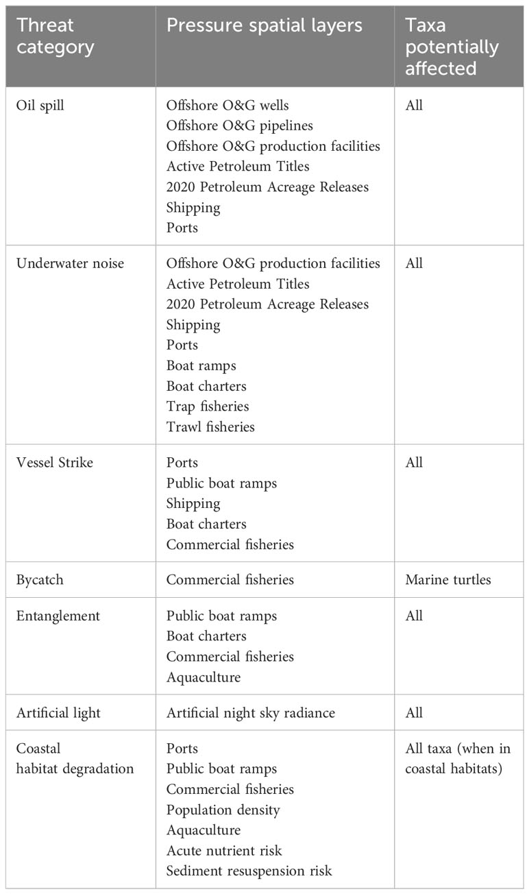
Table 1 Details of threat categories considered in this study and the pressure spatial layers related to each threat and taxa (marine turtles, whales, and whale sharks).

2.4 Pressure spatial layers

Once the threat categories were defined, we searched for existing spatial layers and data that would be representative of those threats (Table 1) and processing of these is described below.

2.4.1 Offshore oil and gas industry

Five pressure spatial layers were available for assessing the main threats associated with the oil and gas (O&G) industry in the study region (Table 1).

We combined spatial layers for O&G wells and pipelines and summed the number of structures in a 10 × 10 km grid cell. We then normalised the count to values between 1 (maximum density of structure) and 0 (no structures present) as a measure of pressure intensity. For offshore O&G production facilities, we created a multi-buffer layer (2 km radius = high exposure; 50 km radius = moderate to low exposure; Gray et al., 1990; Fossette et al., 2021b) to estimate the region of potential high or medium-low intensity of pressure around each production facility (intensity values of 1 and 0.5, respectively). Although the presence of petroleum titles or petroleum acreage releases (Table 1) in a grid cell does not present a direct risk to the marine environment, it provides an estimate of potential future petroleum exploration or extraction and associated activities that can potentially impact marine megafauna. We included only active petroleum titles in the analysis. As title holders are allowed to explore and prospect oil and gas from an active title at any point in time, the presence of a title was given an intensity value of 1 (Table 1). The 2020 acreage releases (i.e., new areas open for bidding for title purchase) were considered a proxy for future oil and gas exploration pressures, and the presence of an acreage release was given an intensity value of 0.5.

2.4.2 Shipping

In Australia, all vessels of 300 gross tonnage and greater undertaking international trips, cargo ships of 500 gross tonnage and greater performing domestic trips, and all passenger ships are required by the Australian Maritime Safety Authority to have automatic identification system (AIS) fitted aboard. The Craft Tracking System (CTS) collects vessel transit data from AIS, with monthly vessel traffic data collected since 2013 made freely available online (Table 1). Vessel traffic data from CTS is provided as monthly point locations for each vessel track with timestamp and vessel ID information. Monthly data between December 2013 and December 2019 were used to map shipping intensity. We chose to combine shipping data from multiple years and not the most recent dataset only as a summary of the last 6 years is likely a better estimate of the current and future shipping density and patterns. The track lines (time series of vessel points) were intersected with the grid and the total number of vessel tracks crossing each grid was summed. The Getis-Ord Gi* statistic was then calculated (Getis and Ord, 1992) using ArcGIS Pro v 2.8 software (ESRI, 2020) to identify significant spatial trends. This statistic was used to determine the intensity of spatial clustering through the resulting z-score and p-value that represents areas where statistically significant spatial clustering of high values or low values occurs. The resulting z-score was used to generate a continuous spatial layer where larger values indicate higher shipping intensity. Scores for each 10 × 10 km grid cell were then normalised between 0 (no shipping) and 1 (maximum shipping) as a measure of shipping pressure intensity.

2.4.3 Boat charter

The boat charter (e.g., licensed companies that provide for-hire boat-based recreational fishing activities) pressure spatial layer was calculated as number of licences that were present in 10 × 10 NM grids provided by the Western Australia Department of Fisheries for the years 2019 to 2022 (Table 1). However, we did not use the most recent effort data (2020 – 2022) due to the effect of COVID-19 on human activity (Huveneers et al., 2021) and instead used the data provided for 2019 only. Grid cell values were extracted to each 10 × 10 km grid cell and normalised between 0 (no boats in a grid cell) and 1 (highest number of boats in a grid cell).

2.4.4 Ports

Based on the area potentially impacted by threats associated (Table 1) with ports and associated coastal structures (Anthony et al., 2013; Rodríguez-Rodríguez et al., 2015; Fuentes et al., 2020), we created multi-layer buffers around Australian port locations to estimate regions of potentially high (2 km radius) and of medium-low (30 km radius) intensity of threats. Intensity values of 1 and 0.5 were assigned to the high and medium-low threat intensity buffers, respectively.

2.4.5 Public boat ramps

Similar to the ports, a 9 km buffer was created around the location of public boat ramps for recreational boating, based on regulations that limit boaters to a maximum distance of 5 NM (i.e., 9 km) from shore. The density of closest population centres, calculated as normalised values between 0 and 1 (see detailed methods for population density below), was assigned to each boat ramp buffer as a proxy of intensity of recreational boating.

2.4.6 Artificial night sky radiance

Artificial night sky radiance data were obtained from the 2015 New World Atlas of Artificial Night Sky Brightness (Falchi et al., 2016) as zenith radiance (mcd/m²) based on the VIIRS Day Night Band in a 30 arcsecond grid. The artificial light layer encompassed radiance from all the main sources of artificial light (e.g., ships, ports, population centres, platforms, gas flares) and thus other pressure spatial layers were not included in the artificial light threat category. We note that the VIIRS sensors underestimate the light produced by white LEDs as they are unable to detect short wavelength blue light. It therefore overestimates other light sources as its sensitivity extends into the near infrared region of the spectrum, where the near-infrared radiation produced by heat sources (i.e., gas flares) is detected and mapped as a component of the light layer and where there is an emission line of the high-pressure sodium lamps that is not visible to human eye (Falchi et al., 2016). Zenith radiance within the Australian EEZ was normalised as intensity values between 0 (no artificial light) and 1 (highest intensity).

2.4.7 Commercial fishing and aquaculture

Commercial fishing effort reported as number of vessels in 10 × 10 and 60 × 60 NM grids were provided by the Western Australia Department of Fisheries for the North-West Marine Region for the years 2019 to 2022 (Table 1). For the same reasons as the boat charter data, only data from 2019 was used in analyses. The number of commercial fishing vessels from logbook data in a 10 × 10 km grid were obtained from the National Environmental Research Program for the North Marine Region. The number of commercial trap and trawl fishing vessels operating in each 10 × 10 km grid cell was summed for each gear type, with the minimum number of fishing vessels in a grid cell considered to be 3 as <3 vessels were not reported by the regulator. Grid cell values were normalised between 0 (no fishing boat in a grid cell) and 1 (highest number of fishing boats in a grid cell).

The spatial layer for aquaculture (Table 1) was obtained as polygons of aquaculture titles from the Western Australia Department of Fisheries. Grid cells where aquaculture titles were present were assigned an intensity value of 1, while the absence of titles were 0.

2.4.8 Nutrient and sediment resuspension

Nutrient and sediment resuspension pressure spatial layers were associated with the threat of coastal habitat degradation (Table 1). Nutrient risk across a 10 × 10 km grid was extracted from Canto et al. (2016) (Table 1). Nutrient risk was derived from metrics of catchment condition and flow metric, and nutrient risk intensity scores were reclassified as high (1), medium (0.75) and low (0.5).

Sediment resuspension risk across a 10 × 10 km grid was calculated as the percentage of time in grid cells that the Shields parameter (i.e., dimensionless shear stress) was greater than 0.25 (Canto et al., 2016) (Table 1). Sediment resuspension scores were reclassified as high (1), medium (0.75) and low (0.5).

2.4.9 Population density

Gridded human population density data were obtained as Usual Resident Population (URP) in 1 km² grid cells (Table 1). These data were used as a measure of population density across Australia from the population census of 2011, the most recent data available at the start of the analysis. The population density data were prepared by creating a 30 km buffer around the borders of population centres (e.g., Anthony et al., 2013), which were delimited by the spatial extent of grid cells with URP > 100 people per km². Population density was then summed within each buffer and values were normalised between 0 (no population recorded in a grid cell) and 1 (maximum population density).

2.5 Threat mapping

All pressures that were considered representative of each of the seven threats as per Table 1 were then overlaid, and normalised grid cell values were summed and normalised again between 0 and 1 (referred to as cumulative pressure) to allow for inter-taxa comparisons. The number of co-occurring pressures (referred to as number of pressures) in each grid cell were also counted and mapped. Hence, the maximum cumulative pressure value for a grid cell for each taxon was 1 and the maximum value for number of pressures varied between 6 and 9 for each taxon as not all taxa were affected by all pressures (Table 1).

We also mapped the distribution of each threat category identified in Table 1 by overlaying all spatial layers that were related to each category and then summed the pressure intensity values and normalised them between 0 and 1 to allow for comparison among threat categories. We also counted and mapped the number of co-occurring threat categories in a grid cell within our study region (0 to 7).

2.6 Threat exposure analysis

Spatial overlap between marine megafauna taxa and pressures was used to estimate two indices of exposure to threats for each taxon in north-west Australia. We adapted the method developed by Halpern et al. (2008) and Maxwell et al. (2013) using the two formulas based on cumulative pressure and occupancy of taxa, and the number of pressures and percentage of animals in a grid cell. As this is an exposure analysis, the risk, magnitude, and frequency of potential impacts, as well as the sensitivity of species, were not considered in the calculations of exposure.

For exposure intensity:

$$EI=S\text{i}\times CP\text{i}$$

Where the exposure intensity (EI) for each taxon is the overlap between taxa occupancy and cumulative pressure in a grid cell. S is the occupancy in a grid cell of taxon i; And CP is the normalised cumulative pressure as the sum of intensity values for all pressures interacting with taxon i. The maximum theoretical value of EI is 1 if the maximum taxa occupancy (1) overlapped with a maximum cumulative pressure (1).

And for exposure in number:

$$EN=N\text{i}\times NP\text{i}$$

Where the exposure in number (EN) for each taxon was the overlap between percentage of individuals and number of pressures in a grid cell. N was the percentage of tagged individuals of taxon i in a grid cell (0 – 100), and NP was the number of pressures that interacted with taxon i in each grid cell. The maximum number of N is 100% but the value of NP varies among taxa. Thus, the maximum theoretical value of EN would be 600 (inter-nesting turtles), 700 (migratory turtles, whales, and whale sharks) or 900 (foraging turtles) if all individuals from each taxon overlapped with all pressures affecting the taxon in a grid cell (maximum of six, seven and nine pressures per taxon, respectively, Table 1). We standardised EN values for each taxon to between 0 and 1 to match the scale of EI values for our cumulative threat analyses, but we also report raw EN values for comparison with the maximum theoretical value for each taxon.

We mapped the exposure (intensity and number) per taxa group to identify areas of high exposure. We then ranked all grid cell values of EI and EN from largest to smallest, and split the cells encompassing the top 50% of the cumulative distribution (i.e. high exposure) from the bottom 50% (after Soanes et al., 2013). We classified the area encompassing the top 50% of cells (highest exposure) as core exposure areas (EI and EN values equivalent to the top 50% quartiles).

We calculated the proportion of the spatial distribution of each taxon within core exposure areas and the proportion of the taxa distributions overlapping with 0 to n co-occurring threats categories (maximum of 7; Table 1). We also calculated the overlap between core exposure areas for each taxon and Australian Marine Parks (Commonwealth regulated), marine reserves (State regulated), Indigenous Protected Areas (co-regulated by Indigenous groups), and Biologically Important Areas (BIAs). In Australia, BIAs are defined as areas where biologically important behaviour occurs and are identified in National Recovery Plans or Marine Bioregional Plans under the EPBC Act (Commonwealth of Commonwealth of Australia, 2012; Commonwealth of Australia, 2015b; Commonwealth of Australia, 2017). These BIAs were extracted from the Australian National Conservation Values Atlas (NCV Atlas; Commonwealth of Australia, 2015a) (http://www.environment.gov.au/webgis-framework/apps/ncva/ncva.jsf). We also assessed overlap with Critical Habitat areas designated by the Recovery Plan for Marine Turtles in Australia (20 km buffer for green and hawksbill turtles and 60 km for flatback turtles, around key rookeries; Commonwealth of Australia, 2017) for inter-nesting turtles.

All analyses used software R version 4.1 (R Core Team, 2019), ArcGIS 10.8 and ArcGIS ArcPro v 2.8 (ESRI, 2020).

3 Results

3.1 Marine megafauna distributions

As our compiled satellite tracking data spanned over multiple years (2000 – 2020), and a reasonable sample size was achieved (median of 49, ranging from 19 to 251 tracks per species; Supplementary Table S2), the calculated distributions were assumed to be representative of the typical spatial distribution of a taxon. All taxa were distributed throughout the study area off north-west Australia and extended into northern Australia, from shallow coastal waters (below the 50 m bathymetric contour) to offshore oceanic areas (beyond the 200 m bathymetric contour) (Figures 2A, B, 3A, B). During inter-nesting, high use areas (occupancy ≥0.5) occurred adjacent to the nesting beaches (Figure 2A) with a large percentage of inter-nesting turtles (>20%) dispersed over larger areas (Supplementary Figure S1A, Supplementary Figure S2F). Distributions of marine turtles during migration and foraging largely occurred over continental shelf waters (<200 m depth) (Figure 2B; Supplementary Figures S3A, B). Only limited migratory movements occurred in oceanic areas (water depths > 200 m) or outside the Australian EEZ (Supplementary Figure S3A, B), with a median water depth of 53 m during migration, ranging from 1 to 6765 m. Areas of highest occupancy (>0.5) during migration mostly occurred in coastal waters off mainland Australia in the Pilbara region and near the nesting sites where turtles were satellite tagged (Supplementary Figures S2A, B and Supplementary Figures S3A, B). Areas of highest occupancy (>0.5) during foraging occurred as discrete grid cells dispersed in coastal waters (Supplementary Figure S1B). The distributions based on the number of turtles in a grid cell mirrored the foraging occupancy distributions, however, high use areas (>15% migrating turtles overlapping in a grid cell, and >4% foraging turtles) were larger for the former (occupancy ≥ 0.5) (Figure 2B and Supplementary Figures S2C, D).

Figure 2

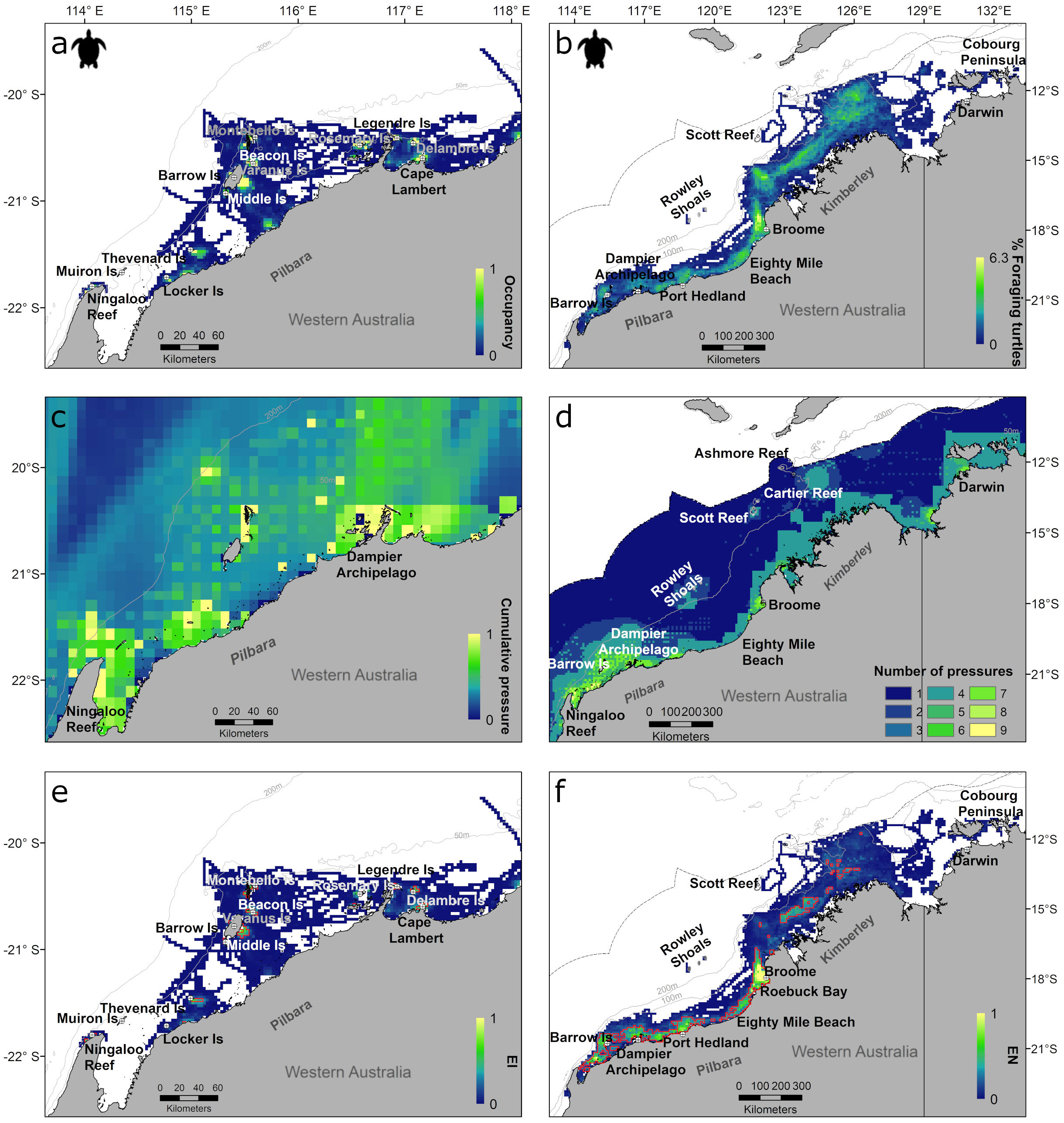
Figure 2 Inter-nesting (left plots) and foraging (right plots) marine turtle distributions based on occupancy index for inter-nesting turtles (A), percentage of tagged foraging turtles in each grid cell (B), cumulative pressure for inter-nesting turtles (C), number of pressures for foraging turtles (D), exposure intensity (EI) for inter-nesting turtles (E) and exposure in number (EN) for foraging turtles (F) in north-western Australia. Outer dotted line represents the Australian EEZ; solid grey lines represent the 20 m, 50 m, 100 m and 200 m depth contours and orange polygons in e) and f) are core exposure (top 50% of cells).

Figure 3

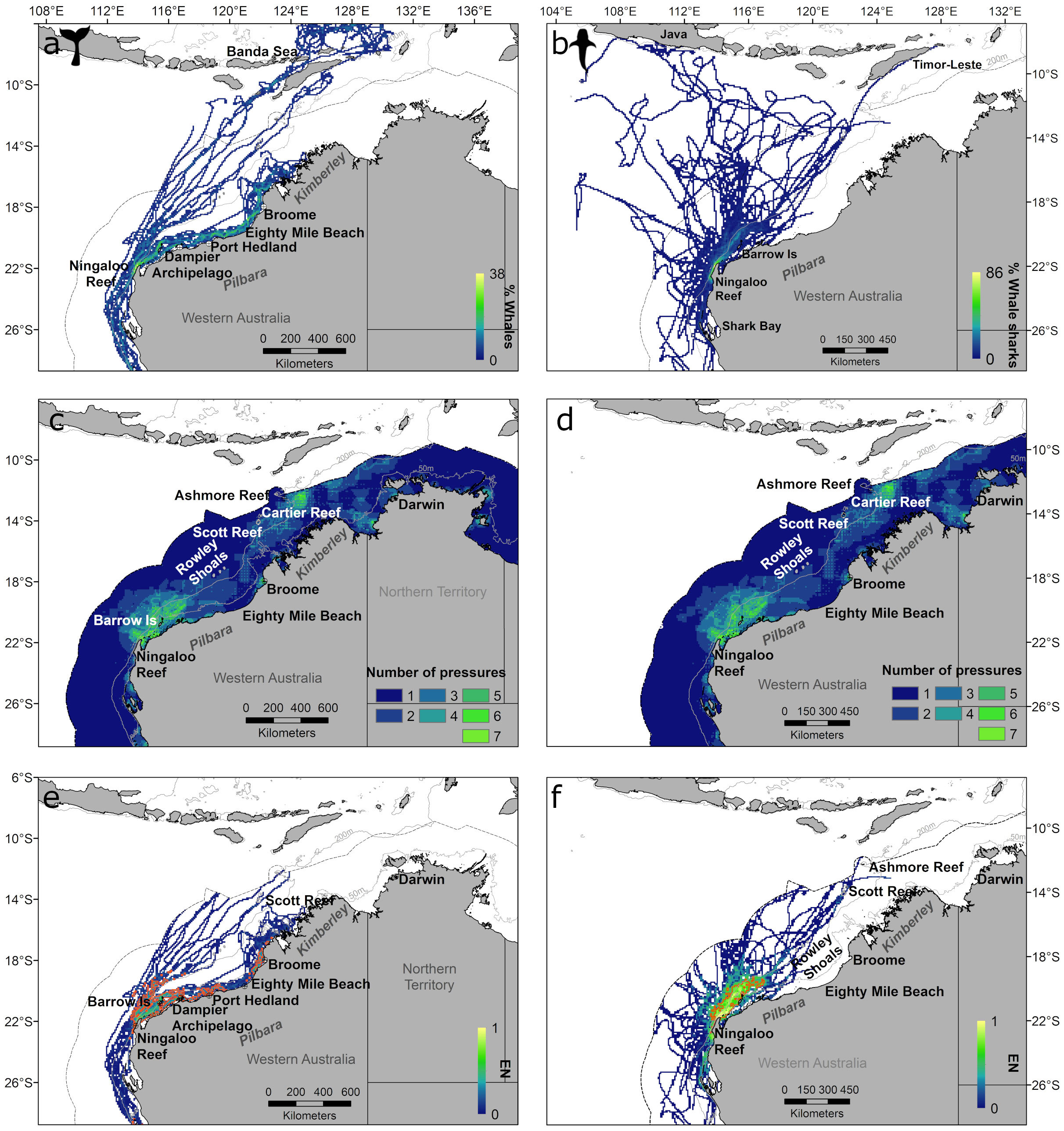
Figure 3 Whale (A) and whale shark (B) distributions based on percentage of tagged animals in each grid cell, number of pressures for whales (C) and whale sharks (D), and exposure in number (EN) for whale (E) and whale sharks (F) in north-western Australia. Outer dotted line represents the Australian EEZ; solid grey lines represent the 50 m and 200 m depth contours and solid orange lines in e) and f) are core exposure areas (top 50% of cells).

There was a clear distinction between use of coastal and oceanic habitats by whales (Figure 3A; Supplementary Figure S4A) that was driven by species and also season, with northerly migrating humpbacks mostly using coastal habitats whereas southerly migrating humpback whales (Bestley et al., 2019) and pygmy blue whales used habitats further offshore with pygmy blue whales movements predominantly occurring at and off the shelf edge. Whales had relatively low occupancy as migration (fast movement) was generally more prevalent than residency behaviour such as foraging, resting and reproduction (slower movement) (Supplementary Figure S4A). Discrete grid cells of higher occupancy occurred near Port Hedland (humpback whales) (Supplementary Figure S5A) and in the Banda Sea (outside Australian EEZ; pygmy blue whales) (Figure 3A). However, a large number of whales overlapped in the Ningaloo Reef region (Figure 3A; Supplementary Figure S5B). Areas with high percentages of whales in a grid cell also occurred along the continental shelf and shelf edge of north-west Australia (Figure 3A; Supplementary Figure S5B).

High occupancy and percentage of whale sharks occurred off Ningaloo Reef where most sharks were tagged (Figure 3B; Supplementary Figure S5A, B), with the largest percentage of sharks (>40%) found in both offshore and inshore waters from Ningaloo Reef to Barrow Island (Supplementary Figure S4B, Supplementary Figure S5D).

All three taxa (turtles, whales, and sharks) overlapped in the continental shelf waters off the Pilbara coast, where most tags (≈66%) were deployed (Supplementary Table S2), but also the southern Kimberley region (Figure 4A). All taxa also overlapped in restricted areas within offshore waters between coastal Pilbara and Scott Reef (Figure 4A). At least two taxa occurred in the southern extent of the study area between Ningaloo Reef and Shark Bay, northern Kimberley and offshore areas in the Pilbara and Kimberley regions (Figure 4A). Areas with only one taxon represented individual migratory paths from tagged individuals or foraging areas used by individual turtles (Figure 4A).

Figure 4

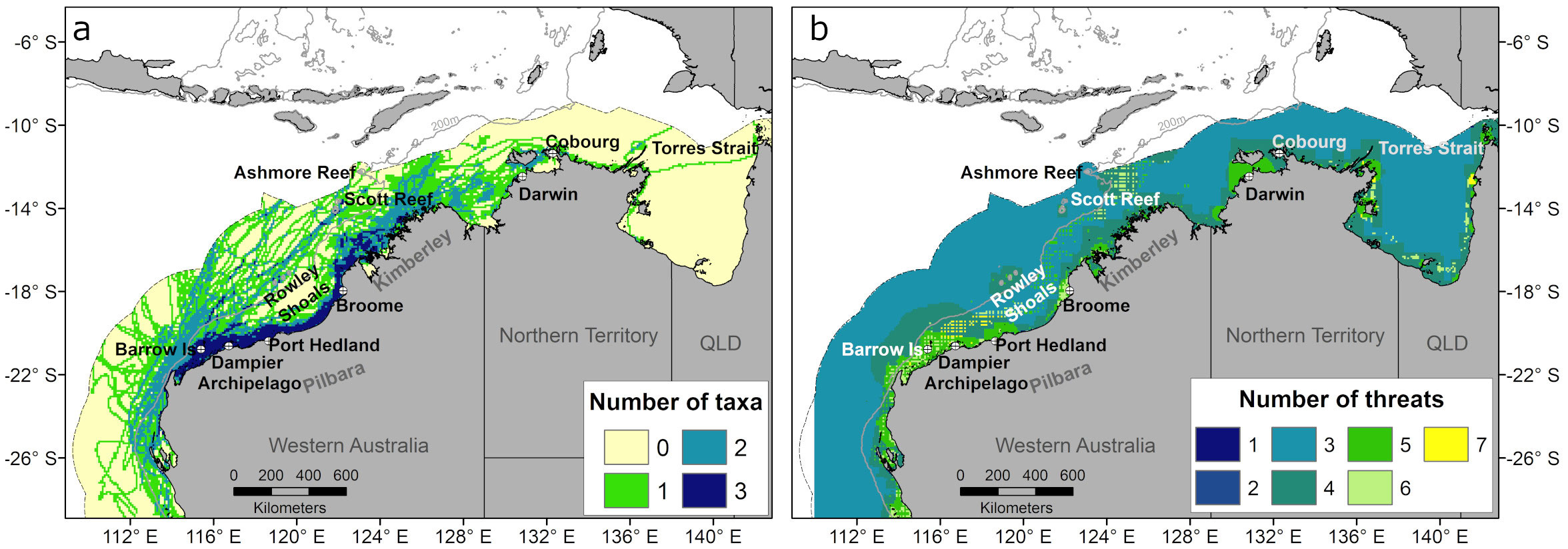
Figure 4 Number of co-occurring taxa (A) and threat categories (B) in each grid cell within the Australian Exclusive Economic Zone.

3.2 Threat mapping

The distribution of cumulative pressures and number of pressures varied with each taxon. For taxa that displayed offshore movements such as whales, whale sharks and migrating turtles, higher cumulative pressures and a larger number of pressures occurred beyond the shelf break in Western Australia (Figures 3C, D; Supplementary Figures S3C, D, S4C, D). For coastal taxa, including nesting and foraging turtles, a higher number of pressures and higher cumulative pressure intensity occurred very close to shore (Figures 2C, D; Supplementary Figures S1C, D). The maximum number of co-occurring pressures was 9 for foraging turtles, 7 for migratory turtles, whales and whale sharks, and 6 for inter-nesting turtles (Figures 2, 3; Supplementary Figures S1, S3).

We also mapped the distribution of each of the seven threat categories listed in Table 1 (Figure 5) and all threats combined (Figure 4B). Coastal modification was limited to within the 50 m bathymetric contour (Figure 5A). Vessel strike, underwater noise and oil spill threats were distributed throughout the Australian EEZ (Figures 5B–D), with highest threat intensity for a vessel strike occurring along intensive shipping routes around the Pilbara region near large ports (Figure 5B). The underwater noise and oil spill threat distribution was greatly influenced by the number of spatial layers for these threats related to the oil and gas industry (Table 1), with higher intensity near the shelf break (200 m bathymetric contour) and offshore waters between the Ningaloo Reef and Rowley Shoals, as well as near Cartier Reef and Joseph Bonaparte Gulf (Figures 5C, D). The distributions for entanglement and bycatch threats largely reflected the spatial footprint of the commercial fishing and aquaculture industries (Figures 5E, F), whereas the threat from artificial light was highest near ports, major towns and at some offshore oil and gas production facilities, e.g., offshore of the northern Kimberley and Pilbara regions (Figure 5G). All seven threats overlapped in shelf waters of the Pilbara coast between Barrow Island and Rowley Shoals and isolated coastal areas in the Northern Territory and Queensland (Figure 4B). Four to six threats categories overlapped in shallow coastal areas and around Rowley Shoals and Scott Reef, whereas most of the offshore waters (> 200 m) had three co-occurring threats (Figure 4B).

Figure 5

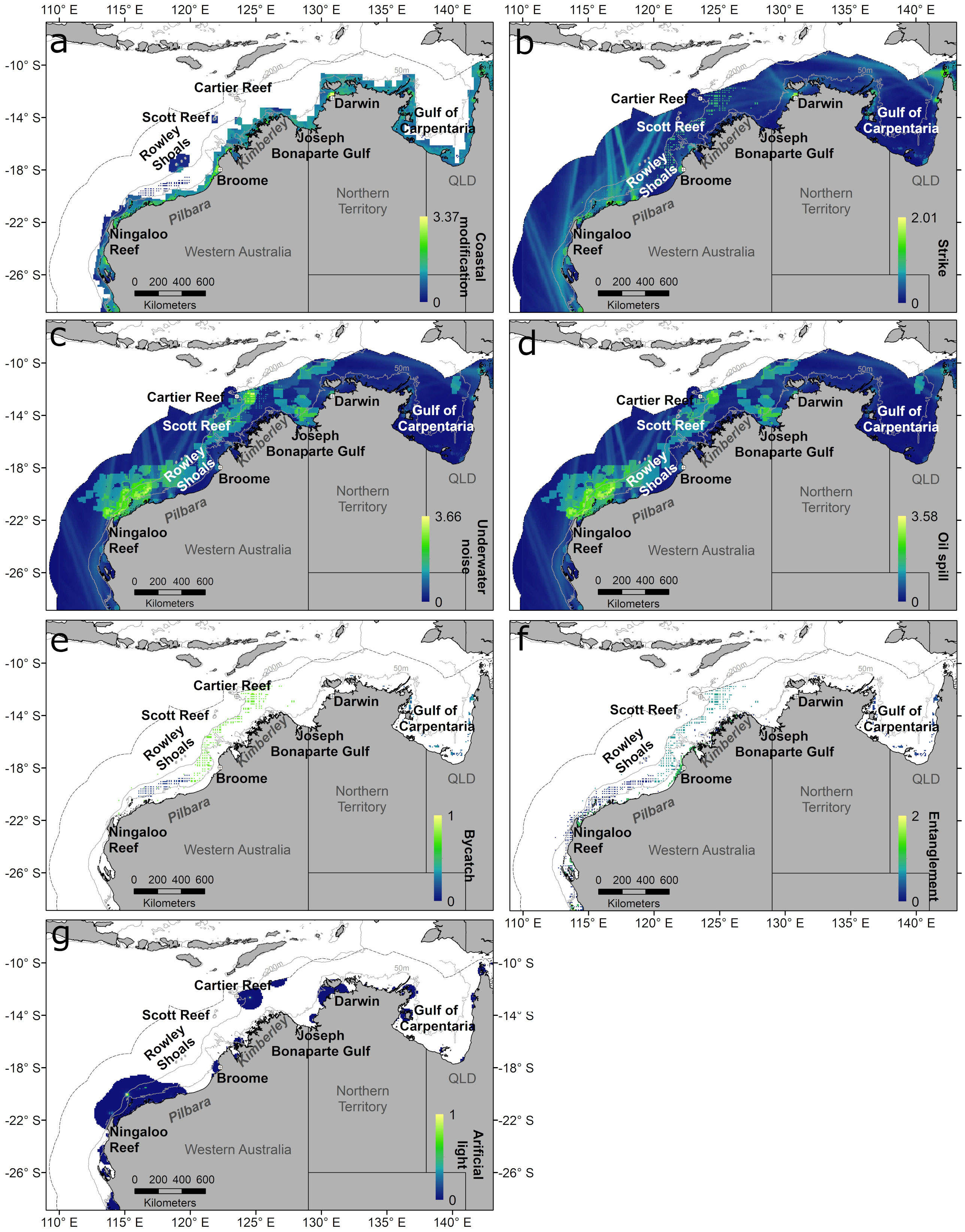
Figure 5 Distribution of each threat category in the study region, within the Australian EEZ (outer dotted line): Coastal modification (A), vessel strike (B), underwater noise (C), oil spill (D), bycatch (E), entanglement (F), and artificial light (G). Grey lines represent the 50 m and 200 m depth contours.

3.3 Exposure analysis

3.3.1 Marine turtle exposure

Core exposure areas (i.e., EI and EN values equivalent to the upper 50% quartiles indicating areas of highest exposure) represented a small percentage of the distribution of marine turtles during all behaviour modes, from a minimum of 1.2% for inter-nesting (EI) to a maximum of 13.5% for foraging (EN) (Table 2; Supplementary Figure S6).

Table 2

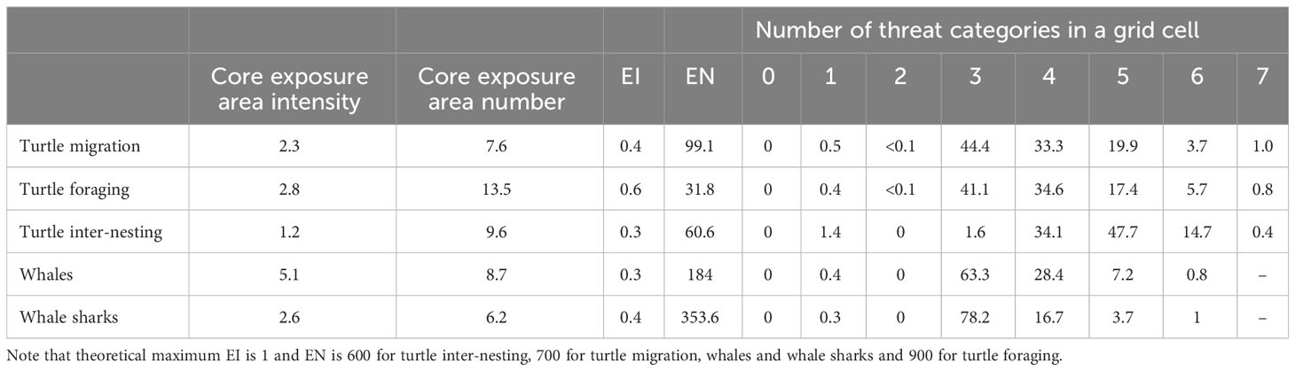
Table 2 Percentage of taxa distribution within core exposure areas (exposure intensity in occupancy and exposure in number), maximum value of exposure intensity (EI) and exposure in number (EN), percentage of whole distribution overlapping with 0 to the maximum threat categories (max = 7 for marine turtles and max = 6 for whales and whale sharks, Table 1).

During inter-nesting, the maximum value of EI was 0.3 (out of maximum of 1) and EN was 60.6 (out of a theoretical maximum of 600) (Table 2). High EI and EN values were concentrated in the Pilbara Region in restricted areas adjacent to nesting beaches, with distinct EI cores defined around rookeries (Figure 2E), and EN cores encompassing multiple nearby rookeries and nesting beaches (Supplementary Figure S1E). The area around Barrow Island showed the highest exposure (EI and EN) (Figure 2E; Supplementary Figure S1E).

During foraging, the maximum value of EI was 0.6 and EN was 31.8 from a theoretical maximum of 900 (Table 2). The highest EN occurred around Roebuck Bay near Broome, followed closely by the area around Barrow Island and the Dampier Archipelago (Figure 2F; Supplementary Figure S7D). Core exposure areas for EN extended over large, semi-continuous areas in the Pilbara region but also in the Kimberley (Figure 2F; Supplementary Figure S7D). Several small core exposure areas were identified for EI that were mostly concentrated in the Pilbara region and restricted to the 50 m bathymetric contour (Supplementary Figure S1F, Supplementary Figure S7C). The highest EI values were observed in Roebuck Bay and inshore of Barrow Island (Supplementary Figure S7C).

During migration, the maximum value of EI was 0.4 and EN was 99.1 (theoretical maximum of 700). Core exposure areas for EN were relatively larger than for EI (Supplementary Figure S3E, F), with one area extending from Barrow Island to west of Turtle Islands in the Pilbara region (both EI and EN) (Supplementary Figures S3E, F, Supplementary Figure S7A, B), and another core area along Eco Beach, Roebuck Bay and Broome (EN only) (Supplementary Figure S3E, Supplementary Figure S7B). Highest exposure (EI and EN) occurred near the Dampier Archipelago (Supplementary Figures S3E, F).

3.3.2 Whale exposure

Whales had a maximum EI of 0.3 and maximum EN of 184 (theoretical maximum of 1 and 700, respectively) (Figure 3E; Supplementary Figure S4E and S6; Table 2). Core exposure areas corresponded to 5.1 and 8.7% of the taxon distribution extent (EI and EN, respectively) (Table 2). For EN, two large core exposure areas were almost continuous from Ningaloo Reef to the southern extent of Eighty Mile Beach, and from the northern extent of Eighty Mile Beach to southern Kimberley, encompassing shelf and offshore waters (Figure 3E; Supplementary Figure S8A). For EI, one large core exposure area encompassed coastal and offshore waters from Ningaloo Reef to Dampier Archipelago, with two other smaller core exposure areas off Port Hedland and Broome and multiple isolated areas located near Shark Bay, Rowley Shoals and Scott Reef (Supplementary Figure S4E, Supplementary Figure S8B).

3.3.3 Whale shark exposure

The maximum EI (0.4 from a maximum of 1) and EN for whale sharks (353.6 from a theoretical maximum of 700) (Table 2; Supplementary Figure S6) occurred at Ningaloo Reef (Figure 3F; Supplementary Figure S4F, Supplementary Figures S8C, D). For EN, a large core exposure area was located near the shore along the Ningaloo Reef region (<200 m bathymetry) expanding out to offshore waters between Northwest Cape and northeast of the Montebello islands along the 200 m bathymetry contour (Figure 3F; Supplementary Figure S8C). For EI, a core exposure area extended along coastal waters (<200 m) along Ningaloo Reef to the offshore off Northwest Cape, and another offshore core exposure area was observed to the northeast of Barrow and Montebello Islands, with a small core exposure area located off Shark Bay (Figure 4F; Supplementary Figure S8D). These areas represented 2.6% and 6.2% of the taxon distribution (EI and EN, respectively) (Table 2).

3.3.4 Overlap with threat categories

We also mapped the number of co-occurring threat categories (i.e., the combined distribution of all pressures associated with a threat category; Table 1, Figure 4B) within the distribution of each taxon (Figure 6). Threats were present in all taxa distributions (Table 2). A maximum of seven threat categories occurred within a grid cell for marine turtles (inter-nesting, migration, and foraging) (Figures 6A–D), indicating that all threats considered here (Table 1) overlapped with marine turtle distributions. Areas of high number of threats within marine turtle distributions were limited to discrete grid cells near the Dampier Archipelago and Barrow Island for all turtle behaviours, but also in deeper waters (>200 m depths) for migrating and foraging turtles (Figures 6A, B). For migrating and foraging turtles, a cumulative total of 98% and 93% of the distributions overlapped with three to five threats, respectively (Table 2). For inter-nesting turtles, approximately 82% of the inter-nesting distribution overlapped with four and five threat categories (Table 2).

Figure 6

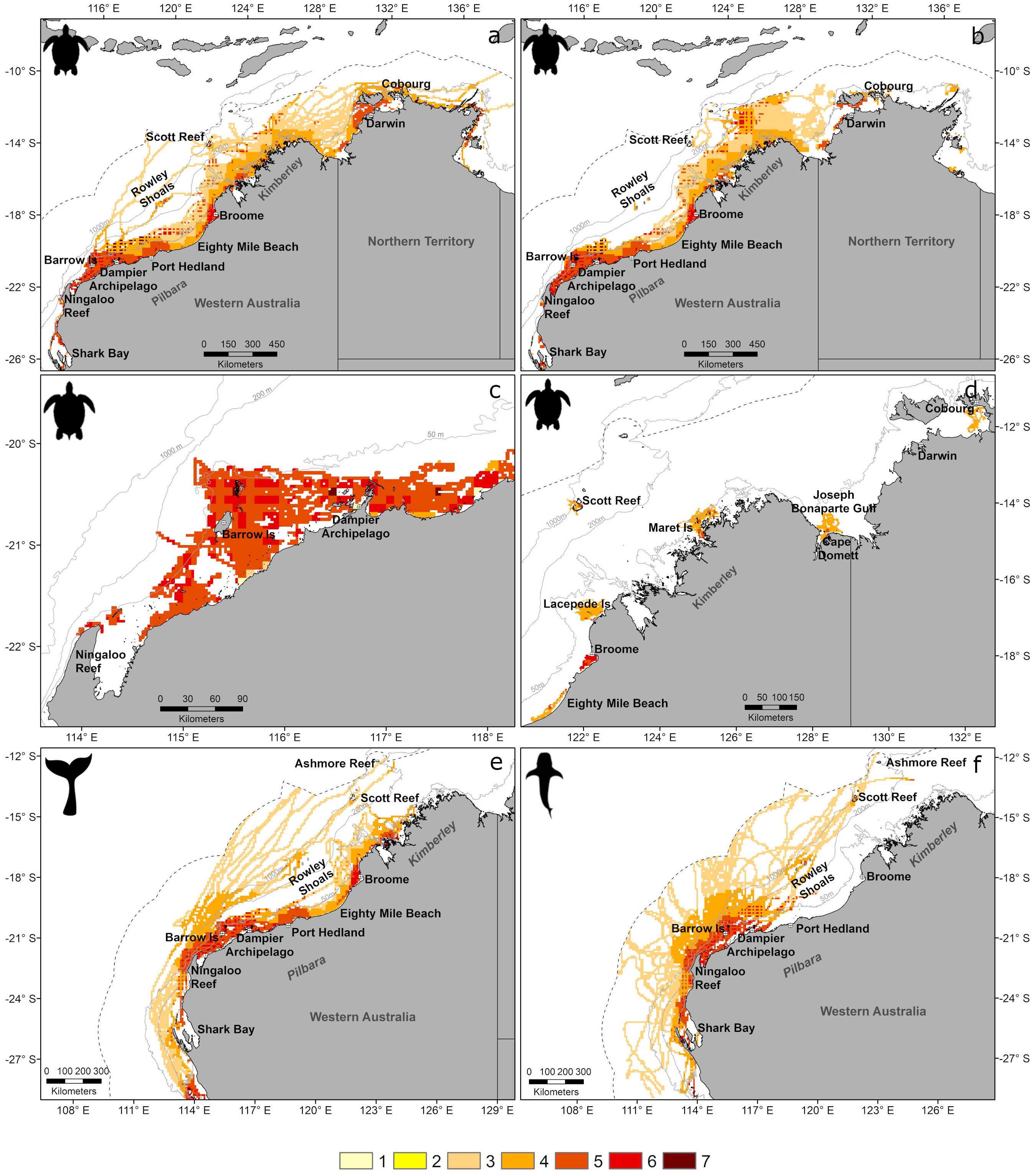
Figure 6 Number of co-occurring threat categories (see Table 1) overlapping with the distribution of each taxon in the study region, within the Australia EEZ (outer dotted line) for foraging turtles (A), turtles during migration (B), turtles during inter-nesting (C, D), whales (E), and whale sharks (F). Grey lines represent the 50 m, 200 m and 1000 m depth contours.

A maximum of six threat categories co-occurred within the distribution of whales and sharks (Figures 6E, F). These represent all threats that we identified to be associated with these taxa, as bycatch by commercial trawl fisheries was considered to affect marine turtles only (Table 1). A larger number of threats (four to six) occurred within the continental shelf (Figures 6E, F) within whale and whale shark distributions. However, 92% and 95% of the distributions (whales and whale sharks, respectively) overlapped with only three or four threats in a grid cell (Table 2). Interactive maps (taxa distributions, threat mapping and exposure) presented here can be accessed in the North-West Atlas (https://northwestatlas.org/node/49001).

3.3.5 Overlap with protected areas

Core exposure areas (areas of highest exposure) of all taxa overlapped with existing BIAs (obtained from the National Conservation Value Atlas) and marine protected areas designated by the Commonwealth and State Governments of Australia (Figure 7). Core exposure areas for marine turtles during migration overlapped with marine reserves (MR) off Barrow and Montebello islands, and with Australian Marine Parks (AMP) in the Pilbara region and Eighty Mile Beach, and Kimberley region (Figure 7A). During foraging, core exposure areas also overlapped with areas designated as foraging BIAs for the marine turtle species included in our study (green, hawksbill and flatback turtles). Similar to migration, core exposure areas for foraging turtles overlapped with multiple coastal marine reserves and AMPs but had large overlap with an offshore AMP in the Kimberley region (Figures 7A, B). Core exposure areas defined for turtle inter-nesting were almost completely encompassed within existing turtle inter-nesting BIAs and Critical Habitat areas around Barrow and Montebello islands, southern Pilbara region near Thevenard Island, and in the Dampier Archipelago (Figure 7C).

Figure 7

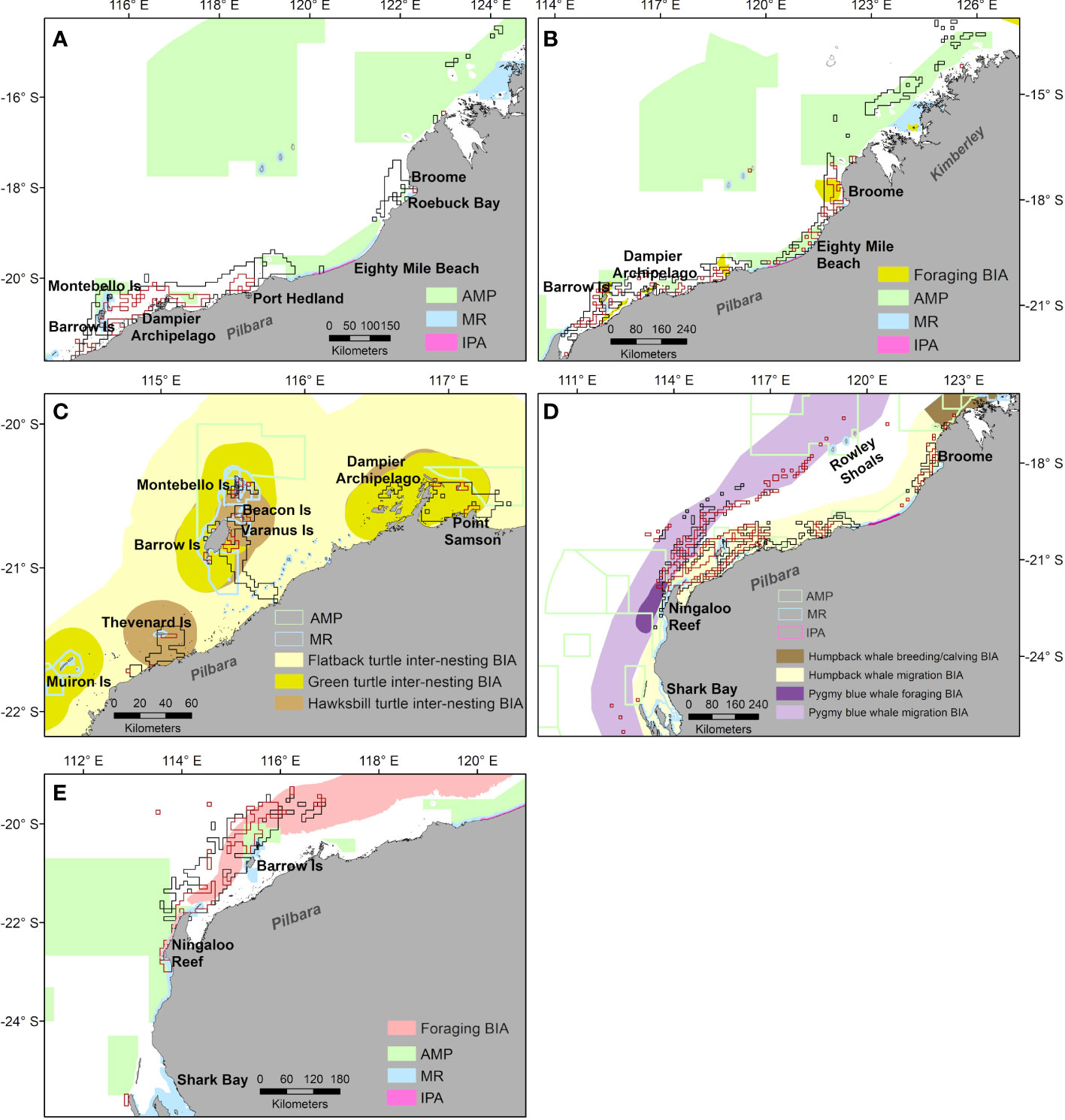
Figure 7 Overlap between core exposure areas defined by exposure intensity (dark red polygons) and exposure in number (black polygons) with marine protected areas and Biologically Important Areas (BIAs) for migrating turtles (A), foraging turtles (B), inter-nesting turtles (C), whales (D) and whale sharks (E). AMP = Australia Marine Park, MR = marine reserves (State regulated), IPA = Indigenous Protected Areas. BIAs for each taxon obtained from the National Conservation Value Atlas https://www.environment.gov.au/webgis-framework/apps/ncva/ncva.jsf.

For whales, core exposure areas overlapped with migratory BIAs for pygmy blue and humpback whales across shelf and off-shelf waters, and with the pygmy blue whale foraging BIA off Ningaloo Reef and the humpback whale breeding and calving BIA in the Kimberley region (Figure 7D). Whale core exposure areas also overlapped with AMPs and MRs off Ningaloo Reef, the Pilbara region, southern Kimberley and an offshore AMP encompassing the Rowley Shoals (Figure 7D).

Core exposure areas for whale sharks overlapped with two foraging BIAs, one off Ningaloo Reef and another in offshore waters (Figure 7E). These high exposure areas also overlapped with protected areas (AMP, MR) off Ningaloo Reef and Barrow Island (Figure 7E).

4 Discussion

Our study collated satellite tracks from 484 individuals of marine turtles, whales and whale sharks encompassing six threatened species to reveal their exposure to anthropogenic threats in north-west Australia. We show that no taxa occurred in the absence of threats within the study area and that areas with existing spatial protections are experiencing high levels of threat exposure. Somewhat encouragingly, a relatively low percentage (up to 14%) of distributions of taxa occurred in high exposure areas. However, these areas still extended over hundreds of kilometres and within them, taxa were exposed to multiple threats. Thus, the cumulative impact of threat exposure on these species must be considered in management planning, especially where taxa display ecologically significant behaviours (e.g., reproduction and foraging) within the area. Importantly, the relatively low percentage of area subjected to high exposure suggests that there is scope to consider management interventions compatible with human activities to reduce such threats. Our results will inform regulators and resource managers assessing proposed industrial activities in waters of north-west Australia, and managers implementing strategies of marine spatial planning. Importantly, our approach provides a model that can be applied at both smaller and larger (including global) spatial and temporal scales.

4.1 Threat mapping

Most species included in our analysis have wide-ranging distributions that extend beyond the Australian EEZ (Wilson et al., 2006; Sleeman et al., 2010; Double et al., 2014; Reynolds et al., 2017; Möller et al., 2020; Ferreira et al., 2021; Thums et al., 2022, Commonwealth of Australia, 2017). However, with the exception of pygmy blue whales, most taxa had highest occupancy, and high percentage of individuals, in coastal waters of north-west Australia, with this area having overlap of all three taxa (Figure 4A).

Overall, number of pressures and cumulative pressures for each taxon were highest on the continental shelf, mid-shelf and slope waters of the Pilbara region (114°E to 117°E), with hotspots around large coastal towns such as Dampier, Port Hedland, Broome and Darwin, where there are large ports and regional towns supporting the resources industry. These high threat values in coastal areas are consistent with the concentration of highest threat and impact levels within coastal zones seen in Australia (Ostwald et al., 2021) and elsewhere globally (Halpern et al., 2009; Maxwell et al., 2013; Trew et al., 2019), as threats resulting from human activities both on land and in the marine environment co-occur in coastal regions (Halpern et al., 2008). In our study area, some offshore areas (>200 m depth) also showed high cumulative pressure and number of pressures for whales and whale sharks. This was due to multiple threats associated with the presence of oil and gas production facilities and commercial fisheries overlapping in this area (Shipping, i.e., artificial light, strike, oil spill and underwater noise).

4.2 Exposure analysis

Areas of high exposure to threats were largely concentrated in coastal waters throughout the Pilbara region and offshore waters across north-west Australia, reflecting the patterns reported for taxa distribution and cumulative threats. When compared to the maximum theoretical exposure scores (1 for EI and 600 – 900 for EN), our exposure values for individual taxon were relatively low to moderate (EI between 0.3 – 0.5 and EN between 32 – 354). This is likely a result of animal distribution showing high occupancy (~1) in a comparatively small area of the total study region thus driving these values (see Figure 2 and Supplementary Figures S1–S4). It also reflects that for most of the extent of taxa distributions we have limited data, particularly for migratory behaviours, resulting in low overlap of individual tracks.

However, even a relatively low to moderate exposure score still implies the presence of multiple threats (Table 2 and Figures 4–6), and the cumulative impact of this exposure could affect animal behaviour and/or population survivorship. For example, the risk of vessel strike is a widespread threat for whale sharks throughout their distribution (Reynolds et al., 2022; Womersley et al., 2022), with strikes occurring in both oceanic and coastal waters. Even within protected areas such as the Ningaloo Reef Marine Park, 39% of sharks identified between 2008 and 2013 exhibited some form of scarring with an increase in number of fresh lacerations year-to-year suggesting increasing boat strikes over time (Lester et al., 2020). Globally, areas of high collision risk (i.e., where core areas of whale shark occurrence and shipping associated threats exist) were positively correlated with reported mortalities of whale sharks due to collision, with vessel strike mortality being probable for at least one tracked shark (Womersley et al., 2022). Thus, even this reported level of exposure may result in negative effects on populations. Risk of vessel strike is also important for whales, with Australia representing 15% of reported vessel strikes involving large whales worldwide (Peel et al., 2018). Additionally, records of entanglement of baleen whales in fishing gear starting in 2010 (Groom and Coughran, 2012) indicate this threat occurs throughout Western Australia, with a maximum record of over 30 whales entanglements in 2013, leading to implementation of gear modification that reduced this statistic to ~9 whale entanglements/year between 2014 – 2017 (How et al., 2021).

Not surprisingly, core exposure areas for coastal species such as foraging and nesting turtles, and humpback whales, occurred in shallow areas of the continental shelf near large cities, ports and areas targeted by coastal fisheries in the Pilbara region. Even large sections of core exposure areas for taxa that display offshore migratory movements were found on the shelf, particularly near Ningaloo Reef, an important seasonal aggregation site for juvenile whale sharks (Wilson et al., 2001; Meekan et al., 2006; Sleeman et al., 2010; Norman et al., 2016) and the deeper waters of the Ningaloo area are an important foraging area along the migratory route of pygmy blue whales in the Eastern Indian Ocean (Double et al., 2014; Möller et al., 2020; Thums et al., 2022). Humpback whales with calves use the Exmouth Gulf area to the east of Ningaloo Reef for resting (Jenner et al., 2001) and neonate calves occur at Ningaloo Reef, with this region possibly representing the southern-most extent of the humpback whale calving grounds along the Western Australian coast (Salgado Kent et al., 2012; Irvine et al., 2017). The importance of the Ningaloo region, a World Heritage Area, for marine megafauna is also evident from the distribution of inter-nesting, migrating and foraging turtles. This area is also used by a wide range of other threatened megafauna not included in this study, such as dugongs (Dugong dugon), reef and oceanic manta rays (Mobula alfredi and birostris), killer whales (Orcinus orca), bottlenose dolphins (Tursiops spp.), Australian humpback dolphins (Sousa sahulensis), Australian snubfin dolphins (Orcaella heinsohni) and several species of cetaceans and sharks (Preen et al., 1997; Sleeman et al., 2007; Allen et al., 2012; Brown et al., 2014; Ferreira et al., 2015; Hanf et al., 2016; Speed et al., 2016; Raudino et al., 2018), but telemetry data for these species are largely absent or else minimal, and/or restricted in spatial coverage.

Additionally, core exposure areas calculated using EN were relatively larger than those of EI, indicating that a large percentage of the tagged animals overlapped with many pressures (at least three or four out of seven) and were consequently exposed to multiple threats (Figure 6). This is because the percentage of individuals is a more conservative metric to define important areas when limited sample size is available (Ferreira et al., 2021; Thums et al., 2022), particularly for the extensive spatial scale used here. As a result, core exposure areas identified using EN are more useful to highlight geographical areas where caution is needed for future management. Our exposure intensity index, however, can easily be used in to analyses of cumulative impact and risk at appropriate spatial scales and for specific species, where other information such as species vulnerability are also accounted for in recognition that impact and vulnerability indices vary with each species (Maxwell et al., 2013) and also life stage. For example, inter-nesting turtles are vulnerable to different threats and at different intensities compared to migratory or foraging turtles (Poloczanska et al., 2009; Fuentes et al., 2011; Hart et al., 2018; Fossette et al., 2021b).

Although core exposure areas represented less than 14% of most taxa distributions, some of these areas extended over ~5° of longitude, spanning hundreds of kilometres and encompassing remote areas on and off the shelf. However, comparatively, in the Gulf of Mexico, 38% of the area used by foraging turtles overlapped with high levels of threats (Hart et al., 2018) and in the Equatorial Guinea, over 25% of suitable habitat for marine mammals had high impact scores (Trew et al., 2019). The relatively low percentage of area exposed to high levels of threats found here in comparison to other highly industrialised regions such as the Gulf of Mexico indicates that management and restrictions of some human activities (e.g., time area closures, boat propellor guards, fishing gear modifications, and restriction of harmful activities within protected areas) have the potential to be considered preemptively. However, we note that many of the activities we assess are of economic and social value, and so a trade-off exists between species protection and human activities. In addition, research prioritisation (e.g., via vulnerability/risk assessments) within this area would likely be feasible at this level of exposure and provide essential information needed for recovery plans and species and spatial management.

The reported exposure of marine turtles, whales and whale sharks to threats occurred despite Australia having a large network of marine protected areas throughout these marine regions. The overlap between core exposure areas and existing spatial protection (Australian marine parks, state-managed marine reserves, and BIAs) indicates that these taxa are still exposed to high levels of threats even when inside the boundaries of designated protection areas. Although some human activities, such as commercial fishing and other natural resource exploration pressures, are excluded from most MPAs, these areas are still exposed to other threats. This includes habitat modification from coastal development, underwater noise from nearby oil and gas production facilities, shipping lanes and recreational boating, as well as artificial light from nearby ports or urban centres. We acknowledge that some impacts of some of these activities may be mitigated (e.g., Oil Pollution Emergency Plan [OPEP] for oil and gas regulations, Ship Oil Pollution Emergency Plan [SOPEP] for large commercial vessels and Bycatch and Discarding Workplans for commercial fisheries), and so a useful next step would be to undertake a cumulative risk assessment of priority areas and species. Although such a process would not be possible across the entire extent of our study area because considerable gaps exist in the understanding of taxa-specific impacts and mitigations of human pressure at spatiotemporal scales relevant to the activity and species distribution (Cordes et al., 2016; Elliott et al., 2019), and thus species-specific risk assessments may be more feasible. Doing so would highlight existing mitigation and areas within species distribution that require further mitigation of the major threats, or to support the design of new areas for protection. This is particularly relevant for threats such as boat strike, entanglement, and coastal modification to migratory humpback whales and marine turtles, especially in marine reserves and World Heritage Areas such as Ningaloo Reef. Additionally, we showed that inter-nesting core exposure areas are almost completely encompassed within turtle inter-nesting Critical Habitat. Considering the importance of these habitats for species survival (Commonwealth of Australia, 2017), fine-scale assessments of cumulative impact and risk could inform on the effectiveness of current mitigation efforts and inform on the need for further mitigation.

Our analysis suggests that the industrial development of north-west Australia is largely responsible for the high threat exposure within the region through intense shipping, oil and gas production facilities, onshore infrastructure, ports and population centres that service their work force. Industrial developments are assessed and regulated through legal frameworks by the States and Territories and/or the Australian Government. An impact assessment process is required for every new development proposal that has the potential to harm a listed threatened species (or habitat) and BIAs available in the National Conservation Values Atlas are often used by regulators to assess the overlap of proposed developments with the distributions of threatened and migratory species. Our detailed analysis will therefore benefit industry by providing distribution maps across behaviours and taxa groups (e.g., Figures 2, 3). This is particularly useful as many existing BIAs have been designed based on limited data combined with expert input rather than quantitative analysis (Thums et al., 2022). Managers will equally benefit from these outputs and the ability to assess and identify areas where a new industrial development might add pressure to an area that is already highly exposed to threats. This is important as impact assessments are usually conducted on an individual project level and, further, existing legislated mitigation and management measures do not take into consideration the potential cumulative impact of multiple co-occurring pressures and projects. Our analysis also highlights areas within megafauna distributions that have lower exposure to threats that could be targeted for the design of new protected areas or enhanced protection to ensure relatively pristine habitats are conserved. For example, low exposure areas within the Kimberley region, as well as the waters off Eighty Mile Beach, were important for turtles and whales, whereas the southern Ningaloo Reef was important for whale sharks and whales (see Figures 2, 3).

Distributions of marine species are dynamic, particularly in the case of highly mobile megafauna, and the definition of spatial distributions can be highly dependent on the sample size of tracked animals (Shimada et al., 2020; Ferreira et al., 2021). It is important to recognise that there are some inherent biases that exist in our tracking datasets, as almost all of our satellite transmitters were deployed within the North-West Marine Region, and some of our tracking datasets were sex and age biased (only adult female turtles) and others seasonally biased (only pygmy blue whales during outward migration) (Figure 1; Supplementary Table S2). Despite attempting to reduce bias towards tagging locations in the calculation of time spent in area and proportion of individuals in grid cells, it is expected that a larger number of tags will be active (and therefore, a larger amount of data is being transmitted) closer to the tagging location (Block et al., 2011), which results in some underestimation of distribution beyond the tagging site. In addition, animal telemetry data provides presence‐only observations with no information about absence or abundance of species. Thus, a lack of movement data in an area does not necessarily mean that it is not used by the species or taxa. This is particularly true when sample sizes of tracking data are low relative to the size of the population, as was the case for whales and whale sharks in our study. Hence, the exposures calculated here are potentially under-estimated. Even for marine turtles, large numbers of tagged animals (n = ~100) may still not be sufficient to describe the full extent of the foraging distribution (Ferreira et al., 2021), however, they are likely to be representative of hotspot areas. For this reason, we did not down-sampled the available tracking data for flatback turtles (n = 251 individuals) relative to the other turtle species considered in this study (n = 96 and 42 individuals for green and hawksbill turtles, respectively). Although the larger flatback turtle dataset may have created a flatback turtle bias in the location of the highest value of turtle exposure, the overall distribution of turtle exposure was not impacted by this bias. Alongside these caveats of sample size and bias, it is important to consider that many of the threats considered here are not static and will likely change in both spatial and temporal extent, as will other threats not accounted for here, such as climate change and marine debris.

Our study focused on threats that are able to be managed at local and regional scales. Although climate change is a major threat for marine megafauna (Halpern et al., 2008; Maxwell et al., 2013; Lewison et al., 2014; Bowler et al., 2020), pressures associated with this threat – including carbon emissions, global industrialisation, large scale agriculture/farming and deforestation – have a global distribution and are not restricted to the marine environment. Associated mitigation actions are subsequently required to be implemented at a much larger scale than the regional context of our study. Similarly, the threat of plastic ingestion for marine megafauna as a result of the concentration of marine debris has been increasingly gaining attention as a widespread, key pressure on species and populations (see review Kühn and van Franeker, 2020). However, spatial data on distributions of marine debris and plastics within the Australian EEZ remains limited (but see Reisser et al., 2013; Olivelli et al., 2020) and detailed mapping at more relevant spatial scales is urgently needed to assess the exposure of marine megafauna to this threat. Once this work is completed in the future it can be incorporated into the spatial threat exposure analysis we present here.

5 Conclusion

Our spatial framework quantifying anthropogenic cumulative exposure of marine megafauna is an important resource for industry, managers and regulators to support improved impact assessments. It will assist in identifying and implementing appropriate management and mitigation actions that will ultimately improve ecologically sustainable development outcomes. Places identified as core exposure areas could be considered as management priority areas and trigger the need for enhanced, targeted mitigation during impact assessment of new industrial proposals. Our cumulative exposure analysis is applicable to a range of other megafauna and human pressures where spatial information is available.

Data availability statement

Publicly available datasets were analyzed in this study. This data can be found here: https://apps.aims.gov.au/metadata/view/912f31de-6a9e-4a3d-8f93-c4a8e4f13592.

Ethics statement

The animal study was approved by University of Western Australia Animal Ethics Committee. The study was conducted in accordance with the local legislation and institutional requirements. Details on ethics approvals for individual datasets are listed in Supplementary Table S3.

Author contributions

MT wrote the proposal and obtained the funding and permits with assistance from MM. LF, MT, SW, SF conceived the ideas anddesigned methodology. LF, MT, SW, MM, VA-G, CA, KB, AD, MD, MG, CJ, MJ, GM, LM, BN, KP, SR, JR, TT, DW, PWi, PWh, SF collected the data. LF and SH analysed the data with assistance from MT, SH, GL, BR, LP. LF, MT, SW, MM and SF led the writing of the manuscript. All authors contributed to the article and approved the submitted version.

Funding

The author(s) declare financial support was received for the research, authorship, and/or publication of this article. This study was conducted as part of AIMS’ North West Shoals to Shore Research Program and was supported by Santos Ltd as part of the company’s commitment to better understand Western Australia’s marine environment. The funder was not involved in the study design, collection, analysis,interpretation of data, the writing of this article or the decision to submit it for publication.

Acknowledgments

AIMS acknowledges the Traditional Owners of Country throughout the northern coast of Western Australia where this North West Shoals to Shore Research Program work was undertaken. We recognise these People’s ongoing spiritual and physical connection to Country and pay our respects to their Aboriginal Elders past, present, and emerging. We acknowledge the Department of Biodiversity, Conservation and Attractions, Pendoley Environmental, Rio Tinto, Chevron Corporation and the INPEX-operated Ichthys LNG Project and Woodside Energy Ltd (Woodside) as Operator for and on behalf of the Greater Enfield Project with Mitsui E & P Australia Pty Ltd and the Browse Joint Venture (BJV) and Conservation International Timor-Leste for making tracking data available. SH undertook the research as part of the ICoAST collaborative project and acknowledge support from the Indian Ocean Marine Institute Research Centre collaborative research fund and partner organisations AIMS, CSIRO, DPIRD and UWA. We also thank Peter Farrell and Christopher Teasdale for project management. CWR thanks the Australian Department of Defence, specifically Wayne Bennett, for the opportunity to conduct pygmy blue whale tagging studies. CWR also thank Rodney Thompson, and Gary Ramsay from L3 Harris and Craig Werley from Sonartech Atlas for their guidance with acoustic detection of whales.

Conflict of interest

Authors AD, CJ, and MJ were employed by the company Centre for Whale Research Inc. Author BN was employed by the company ECOCEAN Inc. Authors LP, KP, PWh, and PWi were employed by the company Pendoley Environmental. Author JR was employed by the company Rio Tinto Iron Ore. Author DW was employed by the company ERM Vietnam.

The authors declare that this study received funding from Santos Ltd. and received data from the corporations listed above. The funder and corporate data providers had the following involvement in the study: they had the opportunity to provide feedback (via comments inserted in the text) on the manuscript, which was addressed by the authors only where the authors considered comments were reasonable and factual, i.e. supported by evidence.

Otherwise, the authors declare the research was conducted in the absence of any commercial or financial relationships that could be construed as a potential conflict of interest.

Publisher’s note

All claims expressed in this article are solely those of the authors and do not necessarily represent those of their affiliated organizations, or those of the publisher, the editors and the reviewers. Any product that may be evaluated in this article, or claim that may be made by its manufacturer, is not guaranteed or endorsed by the publisher.

Supplementary material

The Supplementary Material for this article can be found online at: https://www.frontiersin.org/articles/10.3389/fevo.2023.1229803/full#supplementary-material

References

Allen S. J., Cagnazzi D. D., Hodgson A. J., Loneragan N. R., Bejder L. (2012). Tropical inshore dolphins of north-western Australia: Unknown populations in a rapidly changing region. Pacific Conserv. Biol. 18, 56–63. doi: 10.1071/PC120056

CrossRef Full Text | Google Scholar

Anthony K., Dambacher J., Walshe T., Beeden R. (2013). A framework for understanding cumulative impacts, supporting environmental decisions and informing resilience-based management of the Great Barrier Reef World Heritage Area (CSIRO, Hobart: NERP Decisions Hub, University of Melbourne and Great Barrier Reef Marine Park Authority).

Google Scholar

Avila I. C., Kaschner K., Dormann C. F. (2018). Current global risks to marine mammals: Taking stock of the threats. Biol. Conserv. 221, 44–58. doi: 10.1016/j.biocon.2018.02.021

CrossRef Full Text | Google Scholar

Barnosky A. D., Matzke N., Tomiya S., Wogan G. O. U., Swartz B., Quental T. B., et al. (2011). Has the Earth’s sixth mass extinction already arrived? Nature 471, 51–57. doi: 10.1038/nature09678

CrossRef Full Text | Google Scholar

Bayliss P., Hutton M. (2017). Integrating Indigenous knowledge and survey techniques to develop a baseline for dugong (Dugong dugon) management in the Kimberley: Final Milestone Report of Project 1.2.5 of the Kimberley Marine Research Program Node of the Western Australian Marine Science Institution (Perth, Western Australia: WAMSI).

Google Scholar

Bestley S., Andrews-Goff V., Van Wijk E., Rintoul S. R., Double M. C., How J. (2019). New insights into prime Southern Ocean forage grounds for thriving Western Australian humpback whales. Sci. Rep. 9, 13988. doi: 10.1038/s41598-019-50497-2

CrossRef Full Text | Google Scholar

Block B. A., Jonsen I., Jorgensen S., Winship A., Shaffer S. A., Bograd S., et al. (2011). Tracking apex marine predator movements in a dynamic ocean. Nature 475, 86–90. doi: 10.1038/nature10082

CrossRef Full Text | Google Scholar

Bowler D. E., Bjorkman A. D., Dornelas M., Myers-Smith I. H., Navarro L. M., Niamir A., et al. (2020). Mapping human pressures on biodiversity across the planet uncovers anthropogenic threat complexes. People Nat. 2, 380–394. doi: 10.1002/pan3.10071

CrossRef Full Text | Google Scholar

Breed G. A., Costa D. P., Jonsen I. D., Robinson P. W., Mills-Flemming J. (2012). State-space methods for more completely capturing behavioral dynamics from animal tracks. Ecol. Model. 235-236, 49–58. doi: 10.1016/j.ecolmodel.2012.03.021

CrossRef Full Text | Google Scholar

Brown A. M., Kopps A. M., Allen S. J., Bejder L., Littleford-Colquhoun B., Parra G. J., et al. (2014). Population Differentiation and Hybridisation of Australian Snubfin (Orcaella heinsohni) and Indo-Pacific Humpback (Sousa chinensis) Dolphins in North-Western Australia. PloS One 9, e101427. doi: 10.1371/journal.pone.0101427

CrossRef Full Text | Google Scholar

Canto R., Kilminster K., Lyons M., Roelfsema C. M., Mcmahon K. (2016). Spatially explicit current and future threats to seagrass habitats in Australia. Available at: https://catalogue.aodn.org.au/geonetwork/srv/eng/metadata.show?uuid=0419a746-ddc1-44d2-86e7-e5c402473956.

Google Scholar

Commonwealth of Australia. (2012). Marine Bioregional Plan for the North-west Marine Region (Canberra: Department of Sustainability, Environment, Water, Population and Communities).

Google Scholar

Commonwealth of Australia. (2015a). Biologically Important Areas of Regionally Significant Marine Species (Department of Agriculture, Water and the Environment).

Google Scholar

Commonwealth of Australia. (2015b). Conservation Management Plan for the blue whale - a recovery plan under the Environment Protection and Biodiversity Conservation Act 1999.

Google Scholar

Commonwealth of Australia. (2017). Recovery Plan for Marine Turtles in Australia 2017-2027.

Google Scholar

Commonwealth of Australia. (2020). National light pollution guidelines for wildlife Including marine turtles, seabirds and migratory Sshorebirds.

Google Scholar

Cordes E. E., Jones D. O. B., Schlacher T. A., Amon D. J., Bernardino A. F., Brooke S., et al. (2016). Environmental impacts of the deep-water oil and gas industry: A review to guide management strategies. Front. Environ. Sci. 4. doi: 10.3389/fenvs.2016.00058

CrossRef Full Text | Google Scholar

Double M. C., Andrews-Goff V., Jenner K. C. S., Jenner M. N., Laverick S. M., Branch T. A., et al. (2014). Migratory movements of pygmy blue whales (Balaenoptera musculus brevicauda) between Australia and Indonesia as revealed by satellite telemetry. PloS One 9, 1–11. doi: 10.1371/journal.pone.0093578

CrossRef Full Text | Google Scholar

Double M. C., Gales N. J., Jenner K. C. S., Jenner M.-N. (2009). Satellite tagging of south-bound female humpback whales in the Kimberley region of Western Australia: Field Report to the Western Australian Marine Science Institution.

Google Scholar

Double M. C., Gales N. J., Jenner K. C. S., Jenner M.-N. (2010). Satellite tracking of south-bound female humpback whales in the Kimberley region of Western Australia. Final report. (Hobart: Australian Marine Mammal Centre).

Google Scholar

Dunlop R. A., Braithwaite J., Mortensen L. O., Harris C. M. (2021). Assessing population-level effects of anthropogenic disturbance on a marine mammal population. Front. Mar. Sci. 8. doi: 10.3389/fmars.2021.624981

CrossRef Full Text | Google Scholar

Elliott B. W., Read A. J., Godley B. J., Nelms S. E., Nowacek D. P. (2019). Critical information gaps remain in understanding impacts of industrial seismic surveys on marine vertebrates. Endangered Species Res. 39, 247–254. doi: 10.3354/esr00968

CrossRef Full Text | Google Scholar

ESRI (2020). ArcGIS Desktop: Release 10.8 (Redlands, CA: Environmental Systems Research Institute).

Google Scholar

Esteban N., Mortimer J. A., Stokes H. J., Laloë J.-O., Unsworth R. K. F., Hays G. C. (2020). A global review of green turtle diet: sea surface temperature as a potential driver of omnivory levels. Mar. Biol. 167, 183. doi: 10.1007/s00227-020-03786-8

CrossRef Full Text | Google Scholar

Falchi F., Cinzano P., Duriscoe D., Kyba C. C. M., Elvidge C. D., Baugh K., et al. (2016). The new world atlas of artificial night sky brightness. Sci. Adv. 2, e1600377. doi: 10.1126/sciadv.1600377

CrossRef Full Text | Google Scholar

Ferreira L. C., Thums M., Fossette S., Wilson P., Shimada T., Tucker A. D., et al. (2021). Multiple satellite tracking datasets inform green turtle conservation at a regional scale. Diversity Distributions 27, 249–266. doi: 10.1111/ddi.13197

CrossRef Full Text | Google Scholar

Ferreira L. C., Thums M., Meeuwig J. J., Vianna G. M. S., Stevens J., Mcauley R., et al. (2015). Crossing latitudes-long-distance tracking of an apex predator. PloS One 10, e0116916. doi: 10.1371/journal.pone.0116916

CrossRef Full Text | Google Scholar

Fossette S., Ferreira L. C., Whiting S., King J., Pendoley K., Shimada T., et al. (2021a). Quantifying movement and distribution of the critically endangered hawksbill turtle in the Eastern Indian Ocean. Global Ecol. Conserv. 29, e01713. doi: 10.1016/j.gecco.2021.e01713

CrossRef Full Text | Google Scholar

Fossette S., Loewenthal G., Peel L. R., Vitenbergs A., Hamel M. A., Douglas C., et al. (2021b). Using aerial photogrammetry to assess stock-wide marine turtle nesting distribution, abundance and cumulative exposure to industrial activity. Remote Sens. 13, 1116. doi: 10.3390/rs13061116

CrossRef Full Text | Google Scholar

Fuentes M. M. P. B., Limpus C. J., Hamann M. (2011). Vulnerability of sea turtle nesting grounds to climate change. Global Change Biol. 17, 140–153. doi: 10.1111/j.1365-2486.2010.02192.x

CrossRef Full Text | Google Scholar

Fuentes M. M. P. B., Wildermann N., Gandra T. B. R., Domit C. (2020). Cumulative threats to juvenile green turtles in the coastal waters of southern and southeastern Brazil. Biodiversity Conserv. 29, 1783-1803. doi: 10.1007/s10531-020-01964-0

CrossRef Full Text | Google Scholar

Gaos A. R., Lewison R. L., Wallace B. P., Yañez I. L., Liles M. J., Nichols W. J., et al. (2012). Spatial ecology of critically endangered hawksbill turtles Eretmochelys imbricata: implications for management and conservation. Mar. Ecol. Prog. Ser. 450, 181–194. doi: 10.3354/meps09591

CrossRef Full Text | Google Scholar

Gordon J., Gillespie D., Potter J., Frantzis A., Simmonds M. P., Swift R., et al. (2003). A review of the effects of seismic surveys on marine mammals. Mar. Technol. Soc. J. 37, 16–34. doi: 10.4031/002533203787536998

CrossRef Full Text | Google Scholar

Gray J. S., Clarke K. R., Warwick R. M., Hobbs G. (1990). Detection of initial effects of pollution on marine benthos: an example from the Ekofisk and Eldfisk oilfields, North Sea. Mar. Ecol. Prog. Ser. 66, 285–299. doi: 10.3354/meps066285

CrossRef Full Text | Google Scholar

Groom C., Coughran D. (2012). Entanglements of baleen whales off the coast of Western Australia between 1982 and 2010: patterns of occurrence, outcomes and management responses. Pacific Conserv. Biol. 18, 203–214. doi: 10.1071/PC130203

CrossRef Full Text | Google Scholar

Getis A., Ord J. K. (1992). The analysis of spatial association by use of distance statistics. Geographical Analysis 24, 108–206.

Google Scholar

Halpern B. S., Kappel C. V., Selkoe K. A., Micheli F., Ebert C. M., Kontgis C., et al. (2009). Mapping cumulative human impacts to California Current marine ecosystems. Conserv. Lett. 2, 138–148. doi: 10.1111/j.1755-263X.2009.00058.x

CrossRef Full Text | Google Scholar

Halpern B. S., Walbridge S., Selkoe K. A., Kappel C. V., Micheli F., Agrosa C., et al. (2008). A Global map of human impact on marine ecosystems. Science 319, 948. doi: 10.1126/science.1149345

CrossRef Full Text | Google Scholar

Hanf D. M., Hunt T., Parra G. J. (2016). Chapter eight – Humpback dolphins of western Australia: A review of current knowledge and recommendations for future management. Adv Mar Biol. 73, 193-218.

Google Scholar

Hart K. M., Iverson A. R., Fujisaki I., Lamont M. M., Bucklin D., Shaver D. J. (2018). Marine threats overlap key foraging habitat for two imperiled sea turtle species in the gulf of Mexico. Front. Mar. Sci. 5, 336. doi: 10.3389/fmars.2018.00336

CrossRef Full Text | Google Scholar

Hawkins A. D., Pembroke A. E., Popper A. N. (2015). Information gaps in understanding the effects of noise on fishes and invertebrates. Rev. Fish. Biol. Fish. 25, 39–64. doi: 10.1007/s11160-014-9369-3

CrossRef Full Text | Google Scholar

Hindell M. A., Reisinger R. R., Ropert-Coudert Y., Hückstädt L. A., Trathan P. N., Bornemann H., et al. (2020). Tracking of marine predators to protect Southern Ocean ecosystems. Nature 580, 87–92. doi: 10.1038/s41586-020-2126-y

CrossRef Full Text | Google Scholar

How J. R., de la Mare W. K., Coughran D. K., Double M. C., de Lestang S. (2021). Gear modifications reduced humpback whale entanglements in a commercial rock lobster fishery. Mar. Mammal Sci. 37, 782–806. doi: 10.1111/mms.12774

CrossRef Full Text | Google Scholar

Hückstädt L. A., Schwarz L. K., Friedlaender A. S., Mate B. R., Zerbini A. N., Kennedy A., et al. (2020). A dynamic approach to estimate the probability of exposure of marine predators to oil exploration seismic surveys over continental shelf waters. Endangered Species Res. 42, 185–199. doi: 10.3354/esr01048

CrossRef Full Text | Google Scholar

Huveneers C., Jaine F. R. A., Barnett A., Butcher P. A., Clarke T. M., Currey-Randall L. M., et al. (2021). The power of national acoustic tracking networks to assess the impacts of human activity on marine organisms during the COVID-19 pandemic. Biol. Conserv. 256, 108995. doi: 10.1016/j.biocon.2021.108995

CrossRef Full Text | Google Scholar

Irvine L. G., Thums M., Hanson C. E., Mcmahon C. R., Hindell M. A. (2017). Evidence for a widely expanded humpback whale calving range along the Western Australian coast. Mar. Mammal Sci. 34 (2), pp.294-310. doi: 10.1111/mms.12456

CrossRef Full Text | Google Scholar

Jenner C., Jenner M., McCabe K. A. (2001). Geographical and temporal movements of humpback whales in Western Australian waters. Appea Journal 38, 692-707. doi: 10.1371/journal.pone.0080466

CrossRef Full Text | Google Scholar

Jonsen I. (2020). Package ‘foieGras’: Fit Continuous-Time State-Space and Latent Variable Models for Quality Control of Argos Satellite (and Other) Telemetry Data and for Estimating Movement Behaviour. R package. Available at: https://cran.r-project.org/package=foieGras.

Google Scholar

Jonsen I. D., Bestley S., Wotherspoon S., Summer M., Flemming J. M. (2017). Package ‘bsam’: Bayesian State-Space Models for Animal Movement. R package version 1.1.2, CRAN Repository

Google Scholar

Jonsen I. D., Flemming J. M., Myers R. A. (2005). Robust state – space modeling of animal movement data. Ecology 86, 2874–2880. doi: 10.1890/04-1852

CrossRef Full Text | Google Scholar

Jonsen I. D., Grecian W. J., Phillips L., Carroll G., Mcmahon C., Harcourt R. G., et al. (2023). aniMotum, an R package for animal movement data: Rapid quality control, behavioural estimation and simulation. Methods Ecol. Evol. 14, 806–816. doi: 10.1111/2041-210X.14060

CrossRef Full Text | Google Scholar

Jonsen I. D., Mcmahon C. R., Patterson T. A., Auger-Méthé M., Harcourt R., Hindell M. A., et al. (2019). Movement responses to environment: fast inference of variation among southern elephant seals with a mixed effects model. Ecology 100, e02566. doi: 10.1002/ecy.2566

CrossRef Full Text | Google Scholar

Jonsen I. D., Myers R. A., Flemming J. M. (2003). Meta-analysis of animal movement using state-space models. Ecology 84, 3055–3063. doi: 10.1890/02-0670

CrossRef Full Text | Google Scholar

Kamrowski R. L., Limpus C., Moloney J., Hamann M. (2012). Coastal light pollution and marine turtles: assessing the magnitude of the problem. Endangered Species Res. 19, 85–98. doi: 10.3354/esr00462

CrossRef Full Text | Google Scholar

Kark S., Brokovich E., Mazor T., Levin N. (2015). Emerging conservation challenges and prospects in an era of offshore hydrocarbon exploration and exploitation. Conserv. Biol. 29, 1573–1585. doi: 10.1111/cobi.12562

CrossRef Full Text | Google Scholar

Kennet R., Kitchens J. (2009). Dugong and Marine Turtle Project, Project Final Report to National Heritage Trust Regional Competitive Component (North Australian Indigenous Land & Sea Management Alliance, Darwin).

Google Scholar

Kühn S., van Franeker J. A. (2020). Quantitative overview of marine debris ingested by marine megafauna. Mar. pollut. Bull. 151, 110858. doi: 10.1016/j.marpolbul.2019.110858

CrossRef Full Text | Google Scholar

Lester E., Meekan M. G., Barnes P., Raudino H., Rob D., Waples K., et al. (2020). Multi-year patterns in scarring, survival and residency of whale sharks in Ningaloo Marine Park, Western Australia. Mar. Ecol. Prog. Ser. 634, 115–125. doi: 10.3354/meps13173

CrossRef Full Text | Google Scholar

Lewison R. L., Crowder L. B., Wallace B. P., Moore J. E., Cox T., Zydelis R., et al. (2014). Global patterns of marine mammal, seabird, and sea turtle bycatch reveal taxa-specific and cumulative megafauna hotspots. Proc. Natl. Acad. Sci. United States America 111, 5271-5276. doi: 10.1073/pnas.1318960111

CrossRef Full Text | Google Scholar

Limpus C. J., Fien L. (2009). A biological review of Australian marine turtles (Queensland: Environmental Protection Agency).

Google Scholar

Möller L., Attard C., Bilgmann K., Andrews-Goff V., Jonsen I., Paton D., et al. (2020). Movements, occupancy and behaviour of pygmy blue whales (Balaenoptera musculus brevicauda) satellite tagged in the Great Southern Australian Coastal Upwelling System. Sci. Rep. 10, 21165. doi: 10.1038/s41598-020-78143-2

CrossRef Full Text | Google Scholar

Maxwell S. M., Hazen E. L., Bograd S. J., Halpern B. S., Breed G. A., Nickel B., et al. (2013). Cumulative human impacts on marine predators. Nat. Commun. 4, 2688. doi: 10.1038/ncomms3688

CrossRef Full Text | Google Scholar

McCauley R. D., Fewtrell J., Duncan A., Jenner C., Jenner M.-N., Penrose J., et al. (2000). Marine seismic surveys: analysis and propagation of air-gun signals; and effects of air-gun exposure on humpback whales, sea turtles, fishes and squid (Perth, Australia: Prepared for Australian Petroleum Production Exploration Association).

Google Scholar

Meekan M. G., Bradshaw C. J. A., Press M., Mclean C., Richards A., Quasnichka S., et al. (2006). Population size and structure of whale sharks Rhincodon typus at Ningaloo Reef, Western Australia. Marine Ecology Progress Series, Vol. 319. 275–285.

Google Scholar

Mott R., Herrod A., Clarke R. H. (2017). Resource partitioning between species and sexes in Great Frigatebirds and Lesser Frigatebirds. Auk 134, 153–167. doi: 10.1642/AUK-16-184.1

CrossRef Full Text | Google Scholar

Nelms S. E., Piniak W. E. D., Weir C. R., Godley B. J. (2016). Seismic surveys and marine turtles: An underestimated global threat? Biol. Conserv. 193, 49–65. doi: 10.1016/j.biocon.2015.10.020

CrossRef Full Text | Google Scholar

Noad M. J., Cato D. H. (2007). Swimming speeds of singing and non-singing humpback whales during migration. Mar. Mammal Sci. 23, 481–495. doi: 10.1111/j.1748-7692.2007.02414.x

CrossRef Full Text | Google Scholar

Norman B. M., Reynolds S., Morgan D. L. (2016). Does the whale shark aggregate along the Western Australian coastline beyond Ningaloo Reef? Pacific Conserv. Biol. 22, 72–80.

Google Scholar

Olivelli A., Hardesty B. D., Wilcox C. (2020). Coastal margins and backshores represent a major sink for marine debris: insights from a continental-scale analysis. Environ. Res. Lett. 15, 074037. doi: 10.1088/1748-9326/ab7836

CrossRef Full Text | Google Scholar

Ostwald A., Tulloch V. J. D., Kyne P. M., Bax N. J., Dunstan P. K., Ferreira L. C., et al. (2021). Mapping threats to species: Method matters. Mar. Policy 131, 104614. doi: 10.1016/j.marpol.2021.104614

CrossRef Full Text | Google Scholar

Peel D., Smith J. N., Childerhouse S. (2018). Vessel strike of whales in Australia: the challenges of analysis of historical incident data. Front. Mar. Sci. 5. doi: 10.3389/fmars.2018.00069

CrossRef Full Text | Google Scholar

Pendoley K. L. (2005). Sea turtles and the environmental management of industrial activities in North West Western Australia (Murdoch University).

Google Scholar

Pendoley K. L., Schofield G., Whittock P. A., Ierodiaconou D., Hays G. C. (2014). Protected species use of a coastal marine migratory corridor connecting marine protected areas. Mar. Biol. 161, 1455–1466. doi: 10.1007/s00227-014-2433-7

CrossRef Full Text | Google Scholar

Poloczanska E. S., Limpus C. J., Hays G. C. (2009). “Chapter 2 Vulnerability of marine turtles to climate change,” in Advances in Marine Biology (Academic Press).

Google Scholar

Preen A. R., Marsh H., Lawler I. R., Prince R. I. T., Shepard R. (1997). Distribution and Abundance of Dugongs, turtles, dolphins and other megafauna in Shark Bay, Ningaloo Reef and Exmouth Gulf, Western Australia. Wildlife Res. 24, 185–208. doi: 10.1071/WR95078

CrossRef Full Text | Google Scholar

Queiroz N., Humphries N. E., Couto A., Vedor M., da Costa I., Sequeira A. M., et al. (2019). Global spatial risk assessment of sharks under the footprint of fisheries. Nature 572, 461–466. doi: 10.1038/s41586-019-1444-4

CrossRef Full Text | Google Scholar

Queiroz N., Humphries N. E., Mucientes G., Hammerschlag N., Lima F. P., Scales K. L., et al. (2016). Ocean-wide tracking of pelagic sharks reveals extent of overlap with longline fishing hotspots. Proc. Natl. Acad. Sci. 113, 1582–1587. doi: 10.1073/pnas.1510090113

CrossRef Full Text | Google Scholar

Raudino H. C., Hunt T. N., Waples K. A. (2018). Records of Australian humpback dolphins (Sousa sahulensis) from an offshore island group in Western Australia. Mar. Biodiversity Records 11, 14. doi: 10.1186/s41200-018-0147-0

CrossRef Full Text | Google Scholar

R Core Team (2022). R: A language and environment for statistical computing (Vienna, Austria: R Foundation for Statistical Computing).

Google Scholar

R Core Team (2019). R: A language and environment for statistical computing (Vienna, Austria: R Foundation for Statistical Computing).

Google Scholar

Reisser J., Shaw J., Wilcox C., Hardesty B. D., Proietti M., Thums M., et al. (2013). Marine plastic pollution in waters around Australia: characteristics, concentrations, and pathways. PloS One 8, e80466. doi: 10.1371/journal.pone.0080466

CrossRef Full Text | Google Scholar

Reynolds S. D., Norman B. M., Beger M., Franklin C. E., Dwyer R. G. (2017). Movement, distribution and marine reserve use by an endangered migratory giant. Diversity Distributions 23, 1268–1279. doi: 10.1111/ddi.12618

CrossRef Full Text | Google Scholar

Reynolds S. D., Norman B. M., Franklin C. E., Bach S. S., Comezzi F. G., Diamant S., et al. (2022). Regional variation in anthropogenic threats to Indian Ocean whale sharks. Global Ecol. Conserv. 33, e01961. doi: 10.1016/j.gecco.2021.e01961

CrossRef Full Text | Google Scholar

Roberson L., Wilcox C., Boussarie G., Dugan E., Garilao C., Gonzalez K., et al. (2022). Spatially explicit risk assessment of marine megafauna vulnerability to Indian Ocean tuna fisheries. Fish. Fish. 23 (5), 1180-201. doi: 10.1111/faf.12676

CrossRef Full Text | Google Scholar

Rodríguez-Rodríguez D., Sánchez-Espinosa A., Schröder C., Abdul Malak D., Rodríguez J. (2015). Cumulative pressures and low protection: a concerning blend for Mediterranean MPAs. Mar. pollut. Bull. 101, 288–295. doi: 10.1016/j.marpolbul.2015.09.039

CrossRef Full Text | Google Scholar

Salgado Kent C., Jenner C., Jenner M., Bouchet P., Rexstad E. (2012). Southern Hemisphere Breeding Stock D humpback whale population estimates from North West Cape, Western Australia. Journal of Cetacean Research and Management 12, 29–38. doi: 10.47536/jcrm.v12i1.588

CrossRef Full Text | Google Scholar

Sequeira A. M. M., Heupel M. R., Lea M. A., Eguíluz V. M., Duarte C. M., Meekan M. G., et al. (2019). The importance of sample size in marine megafauna tagging studies. Ecol. Appl. 0, e01947. doi: 10.1002/eap.1947

CrossRef Full Text | Google Scholar

Shimada T., Thums M., Hamann M., Limpus C. J., Hays G. C., Fitzsimmons N. E., et al. (2020). Optimising sample sizes for animal distribution analysis using tracking data. Methods Ecol. Evol. 12 (2), 288-97. doi: 10.1111/2041-210X.13506

CrossRef Full Text | Google Scholar

Sleeman J. C., Meekan M. G., Wilson S. G., Jenner C. K. S., Jenner M. N., Boggs G. S., et al. (2007). Biophysical correlates of relative abundances of marine megafauna at Ningaloo Reef, Western Australia. Mar. Freshw. Res. 58, 608–623. doi: 10.1071/MF06213

CrossRef Full Text | Google Scholar

Sleeman J. C., Meekan M. G., Wilson S. G., Polovina J. J., Stevens J. D., Boggs G. S., et al. (2010). To go or not to go with the flow: Environmental influences on whale shark movement patterns. J. Exp. Mar. Biol. Ecol. 390, 84–98. doi: 10.1016/j.jembe.2010.05.009

CrossRef Full Text | Google Scholar

Soanes L. M., Arnould J. P., Dodd S. G., Sumner M. D., Green J. A. (2013). How many seabirds do we need to track to define home-range area? J. Appl. Ecol. 50, 671–679. doi: 10.1111/1365-2664.12069

CrossRef Full Text | Google Scholar

Speed C. W., Meekan M. G., Field I. C., Mcmahon C. R., Harcourt R. G., Stevens J. D., et al. (2016). Reef shark movements relative to a coastal marine protected area. Regional Stud. Mar. Sci. 3, 58–65. doi: 10.1016/j.rsma.2015.05.002

CrossRef Full Text | Google Scholar

Thums M., Ferreira L. C., Jenner C., Jenner M., Harris D., Davenport A., et al. (2022). Pygmy blue whale movement, distribution and important areas in the Eastern Indian Ocean. Global Ecol. Conserv. 35, e02054. doi: 10.1016/j.gecco.2022.e02054

CrossRef Full Text | Google Scholar

Thums M., Rossendell J., Guinea M., Ferreira L. C. (2018). Horizontal and vertical movement behaviour of adult flatback turtles and spatial overlap with industrial development. Mar. Ecol. Prog. Ser. 602, 237–253. doi: 10.3354/meps12650

CrossRef Full Text | Google Scholar

Thums M., Waayers D., Huang Z., Pattiaratchi C., Bernus J., Meekan M. (2017). Environmental predictors of foraging and transit behaviour in flatback turtles Natator depressus. Endangered Species Res. 32, 333–349. doi: 10.3354/esr00818

CrossRef Full Text | Google Scholar

Trew B. T., Grantham H. S., Barrientos C., Collins T., Doherty P. D., Formia A., et al. (2019). Using cumulative impact mapping to prioritize marine conservation efforts in Equatorial Guinea. Front. Mar. Sci. 6. doi: 10.3389/fmars.2019.00717

CrossRef Full Text | Google Scholar

Tulloch V. J. D., Tulloch A. I. T., Visconti P., Halpern B. S., Watson J. E. M., Evans M. C., et al. (2015). Why do we map threats? Linking threat mapping with actions to make better conservation decisions. Front. Ecol. Environ. 13, 91–99. doi: 10.1890/140022

CrossRef Full Text | Google Scholar

Waayers D., Smith L. M., Malseed B. E. (2011). Inter-nesting distribution of green turtles (Chelonia mydas) and flatback turtles (Natator depressus) at the Lacepede Islands, Western Australia. J. R. Soc. Western Aust. 94, 359–264.

Google Scholar

Waayers D., Tucker T., Whiting S., Groom R., Vanderklift M., Pillans R., et al. (2019). Satellite tracking of marine turtles in the southeastern Indian Ocean: a review of deployments spanning 1990-2016. Mar. Turtle Newslett. 29, 23–37.

Google Scholar

Whiting S. D. (2000). The ecology of immature green and hawksbill turtles foraging on two reef systems in north-western Australia. Marine Ecology Progress Series

Google Scholar

Whittock P. A., Pendoley K. L., Hamann M. (2014). Inter-nesting distribution of flatback turtles Natator depressus and industrial development in Western Australia. Endangered Species Res. 26, 25–38. doi: 10.3354/esr00628

CrossRef Full Text | Google Scholar

Whittock P. A., Pendoley K. L., Hamann M. (2016). Flexible foraging: Post-nesting flatback turtles on the Australian continental shelf. J. Exp. Mar. Biol. Ecol. 477, 112–119. doi: 10.1016/j.jembe.2016.01.015

CrossRef Full Text | Google Scholar

Wilson S. G., Polovina J. J., Stewart B. S., Meekan M. G. (2006). Movements of whale sharks (Rhincodon typus) tagged at Ningaloo Reef, Western Australia. Mar. Biol. 148, 1157–1166. doi: 10.1007/s00227-005-0153-8

CrossRef Full Text | Google Scholar

Wilson S. G., Taylor J. G., Pearce A. F. (2001). The seasonal aggregation of whale sharks at Ningaloo Reef, Western Australia : currents, migrations and the El Nino/Southern Oscillation. Environ. Biol. Fishes 61, 1–11. doi: 10.1023/A:1011069914753

CrossRef Full Text | Google Scholar

Wilson P., Thums M., Pattiaratchi C., Meekan M., Pendoley K., Fisher R., et al. (2018). Artificial light disrupts the nearshore dispersal of neonate flatback turtles Natator depressus. Mar. Ecol. Prog. Ser. 600, 179–192. doi: 10.3354/meps12649

CrossRef Full Text | Google Scholar

Wilson P., Thums M., Pattiaratchi C., Whiting S., Pendoley K., Ferreira L. C., et al. (2019). High predation of marine turtle hatchlings near a coastal jetty. Biol. Conserv. 236, 571–579. doi: 10.1016/j.biocon.2019.04.015

CrossRef Full Text | Google Scholar

Womersley F. C., Humphries N. E., Queiroz N., Vedor M., Da Costa I., Furtado M., et al. (2022). Global collision-risk hotspots of marine traffic and the world’s largest fish, the whale shark. Proc. Natl. Acad. Sci. 119, e2117440119. doi: 10.1073/pnas.2117440119

CrossRef Full Text | Google Scholar

Zangerl R., Hendrickson L. P., Hendrickson J. R. (1988). A redescription of the Australian flatback sea turtle, Natator depressus. Bishop Museum Bull. Zool. 1, 69.

Google Scholar

Žydelis R., Small C., French G. (2013). The incidental catch of seabirds in gillnet fisheries: a global review. Biol. Conserv. 162, 76–88. doi: 10.1016/j.biocon.2013.04.002

CrossRef Full Text | Google Scholar