Toward forest dynamics’ systematic knowledge: concept study of a multi-sensor visually tracked rover including a new insect radar for high-accuracy robotic monitoring

Forest dynamics research is crucial in understanding the global carbon cycle and supporting various scales of forest decision-making, management, and conservation. Recent advancements in robotics and computing can be leveraged to address the need for systematic forest monitoring. We propose a common autonomous sensor box platform that enables seamless data integration from multiple sensors synchronized using a time stamp–based mechanism. The platform is designed to be open-source–oriented, ensuring interoperability and interchangeability of components. The sensor box, designed for stationary measurements, and the rover, designed for mobile mapping, are two applications of the proposed platform. The compact autonomous sensor box has a low-range radar that enables high-detail surveillance of nocturnal insects and small species. It can be extended to monitor other aspects, such as vegetation, tree phenology, and forest floor conditions. The multi-sensor visually tracked rover concept also enhances forest monitoring capabilities by enabling complex phenology monitoring. The rover has multiple sensors, including cameras, lidar, radar, and thermal sensors. These sensors operate autonomously and collect data using time stamps, ensuring synchronized data acquisition. The rover concept introduces a novel approach for achieving centimeter-accuracy data management in undercanopy forest conditions. It utilizes a prism attached to the rover, which an oriented robotic total station automatically tracks. This enables precise positioning of the rover and accurate data collection. A dense control network is deployed to ensure an accurate coordinate transfer from reference points to the rover. The demonstrated sample data highlight the effectiveness and high potential of the proposed solutions for systematic forest dynamics monitoring. These solutions offer a comprehensive approach to capturing and analyzing forest data, supporting research and management efforts in understanding and conserving forest ecosystems.

1 Introduction

Forests are crucial elements of Earth due to their vital ecological, economic, and social roles. Ecologically, forests exhibit high biodiversity and act as habitats for numerous species, promoting ecosystem stability and functioning (Seymour and Busch, 2016). They play a crucial role in carbon sequestration, absorbing and storing substantial amounts of carbon dioxide, thus helping mitigate climate change (Fahey et al., 2010). Forests also contribute to water regulation, soil erosion prevention, and water quality improvement (Ellison et al., 2017). From an economic standpoint, forests support industries such as timber, paper, and pharmaceuticals, providing employment and economic opportunities (Wear, 2002). In addition, forests offer recreational and cultural values, contributing to human wellbeing (Tabbush, 2010). Preserving and sustainably managing forests are, therefore, paramount for the health of our planet and a sustainable future.

Multiple forest research challenges are to be addressed, and environmental monitoring is a central tool for facilitating it. Among challenges, occurring pervasive shifts in forest dynamics are of vital concern. At first glance, deforestation is the most distinguishable concern in the forest dynamics scope. Although forest cover is increasing in many, mainly developed countries, in tropical and subtropical areas, its degradation continues (Pendrill et al., 2019). Forest transitions, i.e., moving from net loss to net gain of forest area, are expanding. Brazil is a remarkable example of attempting to halt deforestation. Regarding forest preservation and restoration strategies, Arroyo-Rodriguez et al. (2020) have concluded that landscapes should contain at least 40% of forest cover to be optimal for forest-dwelling species.

Forest degradation has been extensively monitored worldwide using various remote sensing methods (Gao et al., 2020). The verified Global Forest Change dataset (Galiatsatos et al., 2020) indicates that Africa, South Asia, and South America remain hot spots. Conversely, the situation in temperate and boreal forests appears optimistic regarding the deforestation problem. However, despite national and regional achievements, global deforestation remains challenging. It is worth noting that even well-established remote sensing monitoring in North Europe may occasionally lead to confusion (Ceccherini et al., 2020; Wernick et al., 2021). In addition to deforestation, other less apparent issues associated with forest dynamics require attention. One such challenge is the limited availability of high-resolution data beneath tree canopies, which hampers the accurate assessment of understory vegetation and small-scale structural attributes (Lefsky et al., 2002; Hyyppä et al., 2020). However, this gap can be addressed through modern solutions in robotics and computation.

Another significant environmental monitoring challenge is assessing forests’ role in the global carbon cycle (Pugh et al., 2019). The lack of monitoring data and well-designed models makes it difficult to implement practical policy actions (Mitchard, 2018). Global forest carbon mapping efforts by (Harris et al., 2021) have highlighted the challenge of consistently evaluating mitigation performance across different scales due to the need for standardized data and the utilization of diverse methods and assumptions in worldwide forest carbon monitoring systems (Petrokofsky et al., 2011; Huang et al., 2019; Zhou et al., 2021). The global assessment of the potential of regrowing natural forests to capture additional carbon has encountered issues with data availability and quality, particularly regarding under-crown data (Cook-Patton et al., 2020). The recently recognized complex thermal insulator functions of forests further emphasize the significance of undercanopy measurements (De Frenne et al., 2019).

In addition to the complex forest dynamics questions, concrete factors are strongly considered in the forest monitoring context. Among them, forest fires are one of the main exceptional factors (Boer et al., 2020). Insect pests are another remarkable concrete factor affecting forest dynamics (Jactel et al., 2019). They are expected to exhibit positive responses to climate change with a shorter generation time, higher fecundity, and survival, leading to increased range expansion and outbreaks. Another aspect of forest insect research is conservation. There is a significant need for more systematic insect monitoring techniques, which makes it hard to respond to the pest challenge effectively (Noskov et al., 2021b).

Automatic solutions based on sensor boxes and unmanned vehicles are attracting significant interest recently due to advances in open-source technology supplementing traditional forest monitoring methods (Friess et al., 2019). We would like to draw special attention to the following critical gaps in forest monitoring: first, shortage in effective open-source prototypes of autonomous sensor boxes for static measurements and, second, unmanned vehicle utilization restrictions in challenging forest environments for mobile measurements.

Concerning the first critical gap, forest monitoring with sensor boxes faces challenges, including limited standardization, interoperability, and data quality control (Barrenetxea et al., 2008). It is particularly crucial to have standardization and open-source solutions to enable integration with newly emerging sensors. Although integrating sensor boxes with remote sensing technologies can enhance monitoring efforts, calibration, maintenance, and data processing challenges persist (Nijland et al., 2014). Addressing these gaps requires interdisciplinary collaboration, standardization efforts, and advancements in data analytics. Establishing protocols for data sharing, improving sensor calibration, and developing robust algorithms are essential steps in harnessing the full potential of sensor boxes. By overcoming these challenges, sensor boxes can enhance our understanding of forest ecosystems and support adaptive forest management.

Regarding the second critical gap, practitioners consider two types of vehicles: aerial and ground. Unmanned aerial vehicles (UAVs) equipped with lidar or hyperspectral sensors enable the collection of high-accuracy data in complex forest environments (Wallace et al., 2012). Advanced algorithms and machine learning techniques can computationally process the large-scale datasets obtained from these technologies, facilitating precise characterization of forest attributes (Vandendaele et al., 2021). Although UAVs have gained prominence in forest health monitoring, there is a timely need for ground-based vehicle studies to complement existing techniques. Ground vehicles equipped with sensors, such as lidar or cameras, can provide fine-scale measurements of forest attributes and capture information from close proximity to the forest floor (Nasiri et al., 2021). This approach allows for the detailed monitoring of understory vegetation, root systems, and other ground-level features, contributing to a more comprehensive understanding of forest health and dynamics (Calders et al., 2015). Unmanned ground vehicle (UGV) studies can provide valuable data for the calibration and validation of remote sensing techniques, enhancing the accuracy and reliability of monitoring efforts and offering previously unavailable fine-grained information on understory, forest floor, and forest soil processes (Ghamry et al., 2016; Anastasiou et al., 2023).

Whereas UAV-based solutions have reached a well-established and developed level, UGV-based efforts are still on a lower but rapidly advancing trajectory, presenting multiple unsolved challenges. One of the main challenges is achieving high-accuracy device localization and georeferencing for data collection. The presence of trees causes the multi-path effect in the Global Navigation Satellite System (GNSS) signal, making it challenging to conduct high-accuracy measurements below tree canopies, even with a highly elevated antenna (Brach and Zasada, 2014). In our recent field experience in the forest, we have only achieved GNSS’s FLOAT mode, which provides accuracy on the meter scale, as opposed to the FIXED mode, which enables a centimeter-level accuracy. Other research studies have confirmed this limitation, with studies reporting the best accuracy of 10–15 m (Feng et al., 2021). Accurate UGV positioning is particularly crucial for collecting time-series data. Recent fieldwork has demonstrated the potential to obtain accurate forest attribute information with undercanopy lidar (Hyyppä et al., 2020). In a related study, Qian et al. (2017) achieved a 6-cm accuracy in the XY coordinates [compared to meters in earlier works (Hussein et al., 2013)] by combining GNSS, inertial navigation systems (INSs), and simultaneous localization and mapping (SLAM) calculations. However, the obtained coordinate accuracy varies and is dependent on forest conditions. In addition, the ability to obtain accurate Z coordinates remains uncertain.

Furthermore, the combination of GNSS/INS + SLAM has not yet reached a production level, making it challenging for non-GNSS/INS/SLAM professionals to adopt this approach for broad research. Therefore, we have reservations about the practical feasibility of this approach for our current research.

The present article proposes a novel forest monitoring concept to achieve the highest possible level of detail required for adequate progress in monitoring forest dynamics, carbon cycle–related processes, and specific aspects of forest functionality such as pest management and animal conservation. The widespread adoption of these proposed ideas will significantly contribute to systematic knowledge of forest dynamics. This concept facilitates the collection of fine-grained, high-accuracy time-series data related to forest structure, understory vegetation, forest floor, and animal activity, enabling a comprehensive research framework for large-scale forest monitoring.

First, we suggest the use of a typical sensor box platform. By leveraging popular open-source standard solutions, we can connect a wide range of interchangeable sensors and adopt well-established data acquisition and processing approaches. In addition to commonly used sensors like microphones and cameras, we propose the integration of an experimental radar system, building upon the ideas described in previous works (Noskov et al., 2021a; Noskov et al., 2021b; Noskov, 2022). This radar system allows for continuously collecting high–temporal resolution and compact aggregated data on forest animals, mainly insects. The simultaneous use of cameras and microphones helps to reduce data uncertainty. We demonstrate an autonomous sensor box, a mechanism for data flow integration based on epoch time stamps, and provide samples of collected data to validate the effectiveness of the proposed solution and its potential for expansion into other domains.

Second, we introduce an innovative UGV concept. The developed multi-sensor rover utilizes the aforementioned common sensor platform and data flow integration mechanism. Most notably, we propose a novel method for achieving a centimeter-level accuracy in coordinate detection under forest canopies. In contrast to previous works, our method is based on well-established survey approaches. It involves deploying a reference network within the research area and using a robotic total station to track a prism attached to the rover. This visually tracked rover can potentially provide practitioners with centimeter-accuracy data from multiple sensors.

Finally, we point out that the combination of sensor boxes (primarily for static observations of animal behavior and other high-dynamic or localized forest processes) and unmanned vehicles (mainly for mobile mapping of relatively slow, wide-space phenological conditions) can serve as the foundation for systematic undercanopy forest monitoring. This integrated approach, aiming for very high temporal and spatial accuracy, can also serve as a valuable source of information required to interpret and refine above-crown data obtained from UAVs, satellites, and airborne remote sensing platforms.

2 Elements and design

2.1 Overall concept

Figure 1 illustrates the proposed research schema, which consists of three initial tasks, three deployed and verified platforms, and five partially achieved products. Together, these elements form the research target of attaining systematic knowledge about forest dynamics. The arrows in the figure depict the connections between the conducted and planned research elements. The concept is based on the idea that stationary sensor boxes are utilized for animal monitoring, whereas mobile devices such as UGVs and UAVs are employed for phenology monitoring. Although stationary sensor boxes can provide some information about phenology, their primary focus is animal surveillance. Similarly, although a UGV can collect some data related to animals, its main emphasis is on phenology. For this paper, we do not consider UAVs, but they are scheduled for future work. The following are the initial tasks of forest monitoring, which are further expanded upon:

● animal surveillance;

● mapping of the forest floor, vegetation, and canopy;

● high-accuracy coordinate detection under the canopy.

FIGURE 1

Figure 1 Research infrastructure. Connections of tasks, products, and the research target.

As previously mentioned, animal surveillance relies on stationary sensor boxes equipped with various sensors to detect forest animals, including bats, mammals of all sizes, birds, and invertebrates. Cameras, microphones, and radars are commonly used sensors for this purpose. Cameras are typically configured for motion detection and often require attracting animals to a specific location. Microphones can capture the soundscape, making them particularly effective for ornithology studies. Compact and energy-efficient cameras and microphones are widely used in stationary sensor boxes. However, using cameras and microphones alone has limitations and requires supplementation with other sensors. Recently available radar units show great potential for animal surveillance in autonomous sensor boxes, especially in forest environments. Unlike cameras, radar does not rely on visual contact with the target. It is suitable for nocturnal observations or when targets are hidden by obstacles such as fog or dense vegetation (Taravati, 2018). Compact radar units are emerging in this field and offer promising opportunities for animal surveillance in stationary sensor boxes.

This article presents an autonomous sensor box where radar is a key component. Here, we continue the previous works [Noskov et al. (2021b); especially, Noskov (2021)]. Currently, the radar box aims mainly at nocturnal insects. We also use a camera and microphone, extending the use cases of the sensor box. Prospectively, it can cover a broader range of forest research topics including animal behavior and vegetation/decomposition processes.

A core component of this work is dedicated to forest floor, vegetation, and canopy mapping. We propose a novel solution for conducting systematic research under the forest canopy, focusing on achieving a centimeter-level accuracy. To achieve this, we have developed a multi-sensor rover. Because accurate coordinate detection using real-time kinematic positioning (RTK) GNSS is challenging in forest environments, we propose using an attached prism tracked by a total station that records the prism’s coordinates at short intervals. It is important to note that high-accuracy monitoring beneath the canopy in the forest is currently tricky. However, our proposed approach with a visually tracked rover overcomes this limitation.

For high-accuracy coordinate detection under the canopy, a network of surveyed reference points (reference network) is required to orient the total station. We have transferred the exact coordinates from nearby meadows, where several benchmarks were measured with a sub-centimeter accuracy using RTK GNSS. The oriented total station allows for tracking the rover’s movement and recording its coordinates with approximately a centimeter-level accuracy. Each recorded information, such as photos, point cloud data, audio, and temperature measurements, is geotagged. This means that each photo, for example, is attributed with the XYZ coordinates of the closest recorded point in time from the total station.

All elements of the proposed forest monitoring infrastructure, as shown in Figure 1, are interconnected and converge, intending to increase systematic knowledge about forest dynamics. The sensor box contributes to this knowledge by providing animal monitoring data and serving as a common sensor platform for the rover. The RTK GNSS and total station element is utilized to establish a reference network, essential for measuring trees and orienting the total station to track the rover. The rover collects diverse data related to vegetation phenology and the forest floor, further contributing to our understanding of forest dynamics. Accurate three-dimensional (3D) tree models with semantic information have inherent value, and they are also used for data interpretation by the rover and future adjustments of UAV point cloud data.

In the following subsections, we will provide more details on the elements and design of the developing forest monitoring infrastructure.

2.2 Compact insect radar box

Our extensive review of insect monitoring approaches, focusing on radar techniques, has highlighted the potential of using novel radar solutions for entomology (Noskov et al., 2021b). The review has revealed a significant gap in the availability of compact short-range radar applications for insect research. Although numerous camera-based solutions exist, little attention has been given to compact radar systems. We have proposed using a frequency-modulated continuous-wave (FMCW) compact radar and identified the need for innovative data processing and interpretation methods tailored explicitly for compact radar systems. In addition, we have demonstrated the initial setup of the radar on a rover platform. However, because of the radar unit’s design for larger targets, detecting clear insect signals has proven challenging and unstable. To address this, we have proposed and demonstrated a radar setup integrated with a light trap, which allows us to collect ground-truth information and improve the interpretation of the highly uncertain FMCW radar data.

In our study (Noskov et al., 2021a), we conducted a series of laboratory experiments to investigate how to extract insect signals from the noisy radar data. As a solution, we proposed a novel metric called the Sum of Sequential Absolute Magnitude Differences (SSAMD), which is calculated as follows:

$\begin{array}{ll}SSAMD={\displaystyle \sum _{t=1}^{t_{\max }}{\displaystyle \sum _{c=1}^{c_{\max }}{\displaystyle \sum _{d=0}^{d_{\max }}\left|m_{t,c,d}-m_t-1,c,d\right|}}}& (1)\end{array}$

where t is a time moment or a file number ordered by time; t_max depends on a time interval defined by the user (we use a 1-s interval, so, t_max = 1 s/50 ms = 20. c is a channel number (in our case c ∈ {1, 2, 3, 4}, i.e., all available channels and c_max = 4). d is a distance (an index of a magnitude in a list of magnitudes ordered by the distance); in our case, d_max = 42. m is a magnitude value. One can mention that an absolute difference between the current and previous moment is calculated. SSAMD is simply a sum of all absolute differences.

The SSAMD metric allows for extracting insect presence and biomass information from highly uncertain radar data. This has been validated through multiple laboratory experiments. In addition, several experiments have been conducted using a light diffuser to demonstrate the radar’s capability when integrated with a light trap. The experiments have determined that the insect signal falls within the range of 500 to 3,000 dBm, with lower values indicating the absence of insect targets and higher values likely caused by other sources, such as larger animals.

We have developed an autonomous, compact, and energy-efficient device that integrates a radar unit, a light trap, and several other sensors for fieldwork. Figure 2 illustrates the assembled compact sensor box, the field workflow, a photo of the sensor box taken in the forest, and sample photos captured by the light trap camera. The sensor box measures 40 cm × 30 cm × 25 cm, and the camera holder has a length of 108 cm. The main enclosure is a standard domestic plastic box with a lid with a specially created hole to accommodate the radar unit. Similar to our previous work, we utilize a 60-GHz radar; comprehensive technical details can be found in our previous publication (Noskov et al., 2021a).

FIGURE 2

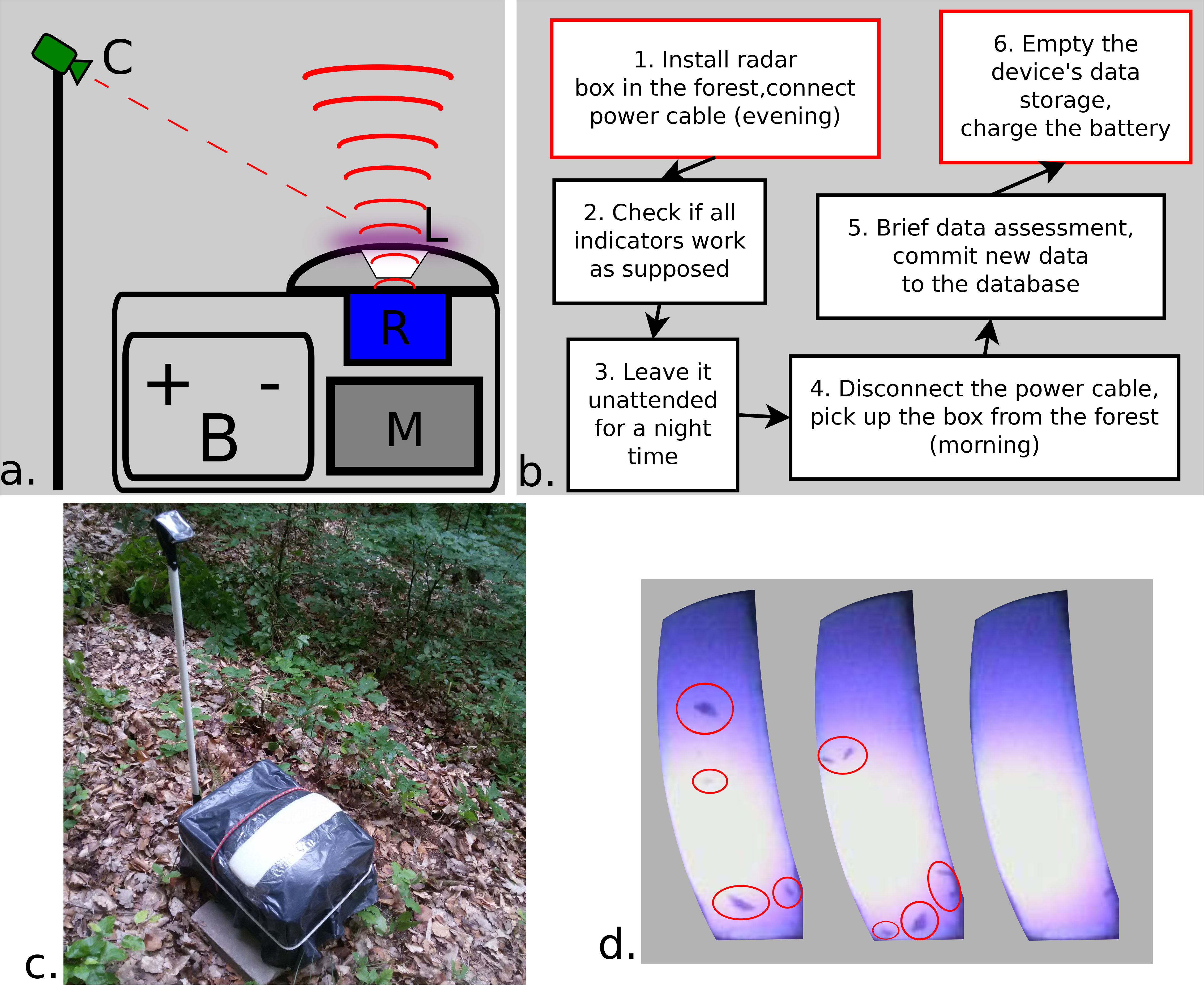
Figure 2 Insect radar. (A) Sensor box’s schema: R, radar; M, managing block (consisting of RaspberryPi, cables, and other components); C, camera with an internal microphone; and L, light trap (ultraviolet LED, reflecting aluminum sheet and a plastic light diffuser); (B) field workflow; (C) operating the insect radar box in the forest (the camera is pointed at the light trap); and (D) examples of light trap’s photos taken on 22 August 2022 (from 23:00 to 23:20).

Figure 2A depicts the components of the designed compact insect radar box. The heaviest component is the 12-V car battery; most of the energy is consumed by the ultraviolet (UV) light-emitting diode (LED). An aluminum sheet reflects the light returning from the bottom of the light diffuser, thereby improving the light trap’s performance, which is equipped with a single LED.

The management block includes a Raspberry Pi, radar data cables, power connections, battery connections, and other miscellaneous wires. The device is powered by a standard car battery using black and red wires with regular clamps. The radar data cables consist of a standard Ethernet cable connected to a radar data cable that runs to the radar unit attached to the lid. The miscellaneous cables include wires for LED management, a polarity protection circuit, an LED driver, and other necessary connections. The polarity protection circuit ensures the radar unit is not damaged due to incorrect battery polarity.

The Microsoft LifeCam HD-3000 web camera, which features a usage indicator (blue light) and an internal microphone, is used in the setup. An Real-Time-Clock (RTC) circuit ensures accurate timekeeping. Two wires connected to pins enable the Raspberry Pi to control the on/off operation of the LED through the DC-DC Constant Current Buck-Boost LED driver. The device is powered by a USB-C cable connected to a USB 12-V–to–5-V converter in the power wire bundle.

In addition, the Raspberry Pi is programmed to shut down the device at a specific time in the morning (usually 09:00) to prevent unnecessary battery discharge. Therefore, the battery must be charged or replaced almost daily, which requires manual intervention. A person needs to retrieve the device in the morning, charge it during the day, upload the collected data, free up disk space if necessary, bring it back to the forest in the evening, and start the radar box. This workflow (also depicted in Figure 2B) typically requires at least 1 h per day (approximately half an hour in the morning and half an hour in the evening). Solar panels can be utilized in the future, eliminating the need for manual intervention in charging the battery to simplify the workflow.

2.3 Multi-sensor visually tracked rover

Whereas drones remain very popular in forest monitoring, rovers show high prospects due to several advantages. Using rovers is beneficial because it enables us to apply multiple sensors and conduct accurate low-viewpoint large-scale forest mapping. In addition, an acquired rover can carry relatively heavy sensors (such as the discussed insect radar box) and has good maneuverability in the forest.

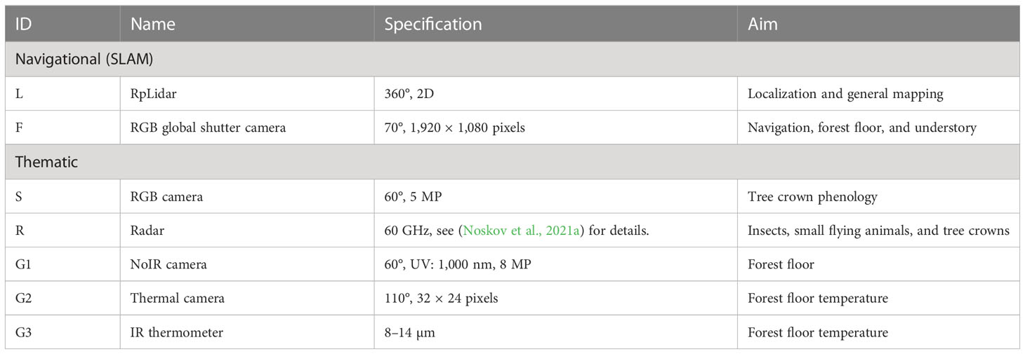
We use a Jackal UGV produced by Clearpath Robotics (Dataset, 2023b). Figure 3 introduces the proposed rover design. Notice that the rover’s top black lid size in the view from above is 48 cm × 32 cm. Table 1 lists the installed sensors. Our rover setup conceptually consists of two main blocks: navigational and thematic. Both have separate computers with connected sensors. All sensors are attached to the top lid of the rover (see Figure 3A).

FIGURE 3

Figure 3 Rover’s schema (A). Navigational block: P, 360° prism; L, RpLidar; and F, front camera (RGB global shutter cameras). Thematic block: S, sky-oriented camera with a flash light and an attached microphone; R, low-range radar; and G, ground-oriented sensors (No Infrared filter (NoIR) camera, infrared thermometer, and thermal camera). Rover’s field workflow (B).

TABLE 1

Table 1 Rover’s sensors.

2.3.1 Navigational sensors

The navigational block of the rover is responsible for performing SLAM tasks, which involve tracking the rover’s location and creating a map of the environment. This block consists of the rover’s internal computer and two connected sensors: RpLidar, and infrared and Red-Green-Blue (RGB) global shutter cameras.

The RpLidar S1 (Dataset, 2023c) is a portable time-of-flight laser range scanner. It utilizes time-of-flight ranging technology, which ensures that the ranging resolution remains consistent regardless of the distance. The device has a range radius of 40 m and is designed to minimize interference from solid daylight. The RpLidar S1 offers stable ranging and high-resolution mapping performance in outdoor environments.

The front camera of the rover is the Intel RealSense Depth Camera D435 (Dataset, 2023a). This camera is known for having the most expansive field of view among all Intel RealSense cameras. It also features a global shutter on the depth sensor, making it suitable for fast-moving applications. The D435 is a stereo solution that provides high-quality depth information for various applications. Its wide field of view is particularly advantageous in robotics, augmented reality, virtual reality, and other scenarios where capturing a large portion of the scene is crucial. The camera has a range of up to 10 m, making it well-suited for forest monitoring applications.

The RpLidar and the front camera enable prospective autonomous navigation in the forest. However, because the rover is operated manually using a wireless controller, these sensors are primarily utilized for general mapping. This includes mapping trees, obstacles, vegetation, understory, and the forest floor.

2.3.2 Thematic mapping sensors

The thematic mapping sensors consist of sky- and ground-oriented sensors connected to the Raspberry Pi.

As described earlier, the radar unit has been initially designed for insect monitoring (Noskov et al., 2021a). However, in this work, we have repurposed it for phenology monitoring, specifically observing tree crowns. As the fieldwork took place during the leaf-fall season (October to November), we aimed to capture the variable radar reflections resulting from the changing conditions of the tree crowns. We expect stronger radar signals in the earlier measurements and weaker signals in the later measurements. The detailed results of this field campaign will be published in future works.

The sky-oriented camera, HBV-1825 FF Camera Module, provides a high-definition image of the tree crowns. It enables us to observe detailed crown changes throughout the leaf-fall period. In addition, this camera has the potential to capture nocturnal species, as discussed in (Noskov et al., 2021b).

The internal microphone records the measurement conditions, such as the rover’s movement and any potential noise impact (e.g., road noise). However, its primary purpose is separate from the thematic mapping tasks.

Moving on to the ground-oriented sensors, we have the Raspberry Pi NoIR Infrared Camera Module 8MP v2.1 (Dataset, 2022), the Optris CT Infrared-Thermometer (Dataset, 2021), and the MLX90640 IR Array Thermal Imaging Camera (Shaffner, 2021). These sensors are focused on the forest floor and ground-level observations.

The infrared camera captures visible patterns of the forest floor, including fallen leaves, grass, moss, and rotting wood. The accurate positioning data obtained from the rover will be valuable for advanced research on forest soils, microhabitats, and forest floor microbiomes. The infrared thermometer measures the temperature of the observed ground patch, providing additional information for analysis. The NoIR infrared camera could be used for observing nocturnal processes on the forest floor.

Finally, the thermal imaging camera produces thermal maps of larger ground patches. It aims at a point on the ground located 1 m behind the rover, allowing for the creation of accurate thermal forest time-series maps. By calculating the average temperature, we can collect temperature point data, where each point represents a wide area behind the rover.

These thematic sensors are positioned along the symmetry axis of the rover. The RealSense Depth Camera is situated at 6 cm from the front of the rover, followed by the HBV-1825 FF Camera at 11 cm, RpLidar at 19 cm, radar at 31 cm, and the ground-oriented sensors at 46 cm from the ground. These sensors record valuable multi-source data, which require a novel merging and positioning approach that we will discuss in the following sections.

Given the challenges of the forest environment, such as lack of GNSS signal, poor GSM coverage, obstacles, and low accessibility, we propose three primary principles for UGV high-detail multi-sensor monitoring in this article: autonomy, time-stamp synchronization, and visual tracking. These principles aim to address the specific problems of systematic monitoring in forest environments.

2.3.3 Autonomy and time-stamp synchronization

We also adopt the design solutions introduced for the insect radar box for the UGV. Moreover, we have designed the rover using discussed autonomous monitoring approach. The rover drives manually with a wireless controller. However, all sensors are preconfigured in lab conditions and are not intended (although it is possible if needed) to be manipulated in the field. They all start recording data automatically with the start of the rover and shut down when it is powered off.

We use three unconnected computers (Raspberry Pi, the rover’s internal computer, and the total station’s tablet) to collect various data sourced from multiple sensors; these data are merged using exact time stamps (epoch seconds). Before starting field measurements, we ensure that the clocks of all computers are synchronized perfectly. In our case, we accept when the clock deviation does not exceed one second. All data slices collected by sensors are addressed with an epoch-seconds time stamp. This makes it possible to merge data residing in the different computers correctly afterward.

2.3.4 Prism for visual tracking

In our forest test bed, obtaining a satisfactory signal accuracy is only possible in meadows and specific segments of roads that cross the forest. The accuracy achieved in our research is measured in meters or tens of meters and renders the collected data unsuitable for high-detail time-series analysis. To overcome this limitation, we have adopted visual tracking using a robotic total station and a prism installed on the rover, enabling a centimeter-level spatial accuracy.

The visual tracking process requires an oriented robotic total station and a 360° prism attached to the rover. Robotic total stations allow for automatic prism tracking and automatic recording of coordinates at a specified time or distance intervals. The environmental illumination conditions do not affect the ability to track the rover; the performance is more or less the same under dark and light conditions.

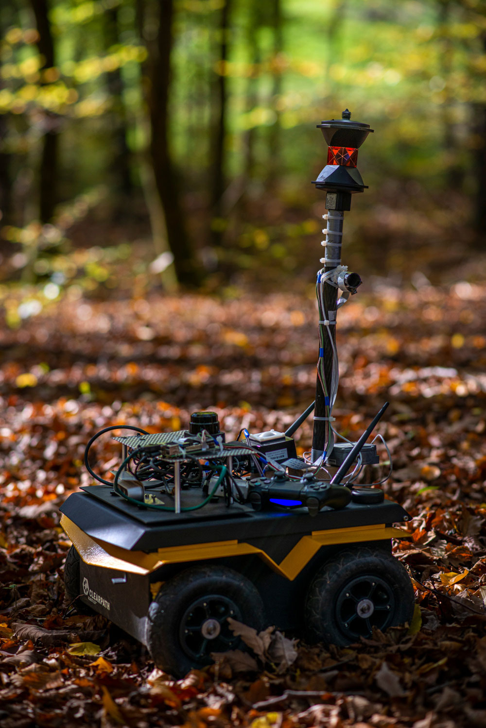
The rover is equipped with a prism holder on the same pole as the thematic mapping sensors, where a 360° prism can be securely fixed. Using the robotic total station, this prism enables automatic tracking of the rover’s coordinates at very short intervals, with an accuracy of approximately 2 cm. Figure 4 illustrates the fully equipped rover, ready for measurements, with the prism mounted on the holder.

FIGURE 4

Figure 4 Operating the rover.

The total station is oriented using a dense reference network established in the key area to ensure accurate data positioning. Correct orientation of the total station is crucial for achieving accurate data collection. The following section will provide further details on this topic.

3 Deployment and demonstration

3.1 Study area

The study area is located approximately 7 km North-West of Marburg in Hesse, Germany, near the Caldern district. The area is characterized by a typical German forest composition, with the following tree species distribution: 60% Fagus sylvatica (European beech), 30% Quercus sp. (oak), and 10% Carpinus betulus (European hornbeam) and other species. The total area covers approximately 20 hectares.

Within this study area, we focused on a smaller, more detailed investigation in the central part. This area spans approximately 5 hectares and encompasses a range of elevation differences, from 256 m above sea level (AMSL) to 275 m AMSL. To capture comprehensive data, we conducted tree measurements using a total station and collected data using a multi-sensor rover. The area of interest is highlighted in Figure 5.

FIGURE 5

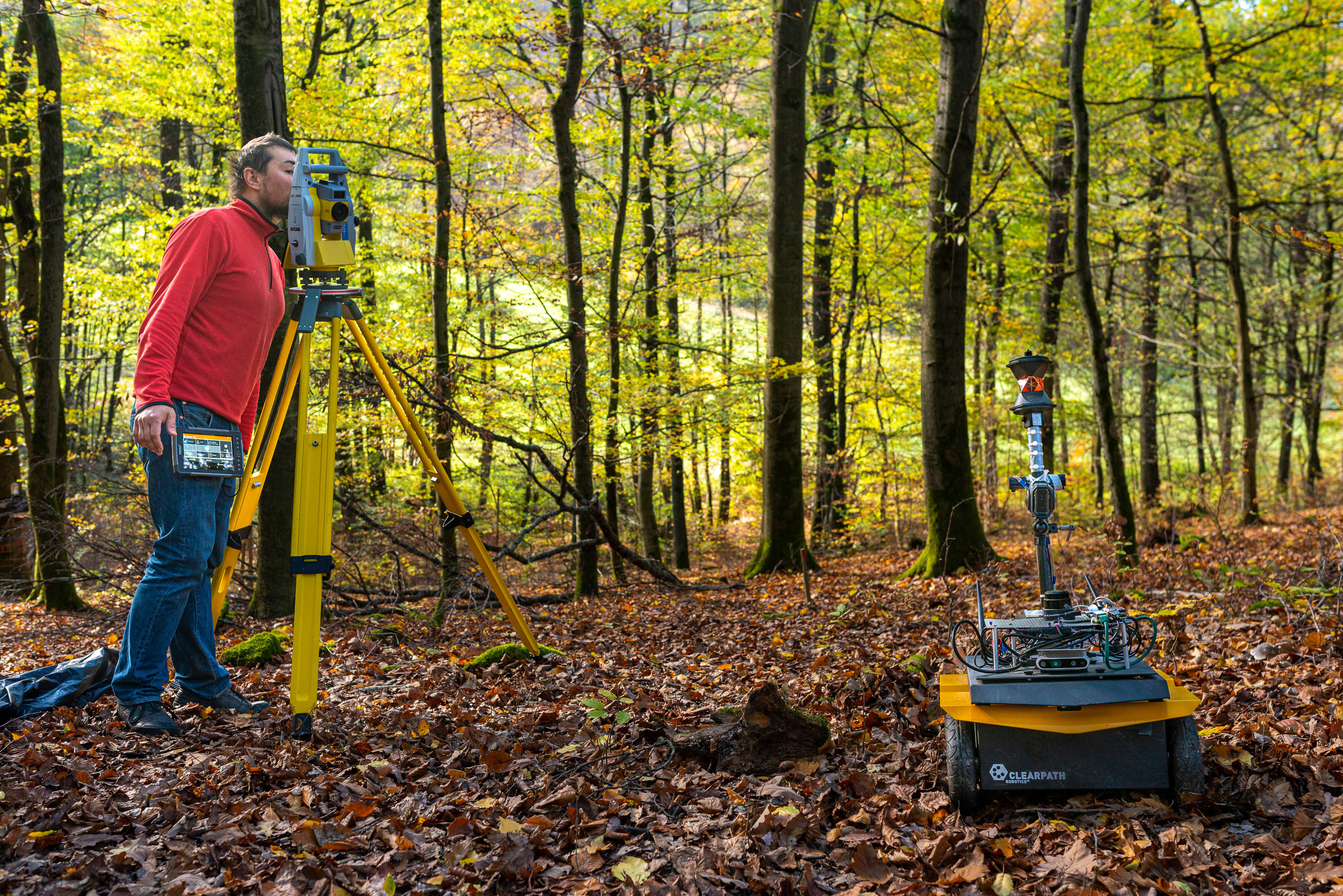
Figure 5 Research area map. Coordinate system: EPSG 32632 (WGS 84/UTM Zone 32N). Satellite imagery of Bing maps.

In addition, regular UAV flights were conducted, capturing RGB point clouds of the entire study area. These aerial data provide an overview of the forest structure and composition.

3.2 Insect radar sensor box

The sensor box has been operational during the warm seasons of 2021 and 2022, specifically during no-rain nights from 20:00 to 09:00, within the vicinity of the automatic weather station in the forest area. This location allows for a comparison of insect radar data with the comprehensive meteorological data collected by the station, as weather conditions significantly impact insect flight behavior. The collected data span long time series, including light trap photos taken at a 5-s interval and radar frequency data captured at a 0.02-s interval, which is used for calculating the SSAMD values over a 1-s interval. These time series enable the calculation of insect presence and biomass information, with ground-truth validation from the light trap photos.

Table 2 provides a summary of the data collected in 2021 and 2022, comprising a total of 66 observation nights (35 in 2021 and 31 in 2022). Each night’s dataset includes radar frequency data and light trap photos. Starting from August 2022, the device also records audio from the camera’s internal microphone, primarily to filter out non-insect signals and noise from larger animals (e.g., badgers) or precipitation effects.

TABLE 2

Table 2 Overview of insect radar data collected in 2021 and 2022.

Figure 6 presents an example of the measured SSAMD values over a 20-min period. In our previous work (Noskov et al., 2021a), we determined that insect targets typically fall within the SSAMD interval of 500 to 3,000, with values above 3,000 considered suspicious and likely caused by larger targets (e.g., bats). In the provided example, most of the SSAMD values indicate insect presence. However, there are three instances where the SSAMD exceeds 3,000, suggesting the potential presence of larger targets like bats. As the light trap attracts various insects, it also attracts bats. It is essential to carefully examine peaks above 3,000 to determine whether they are due to bats or other larger targets. In addition, the impact of dew, fog, and rain on the radar signal needs further investigation, which can be facilitated by the weather station’s data for filtering out interrupted data.

FIGURE 6

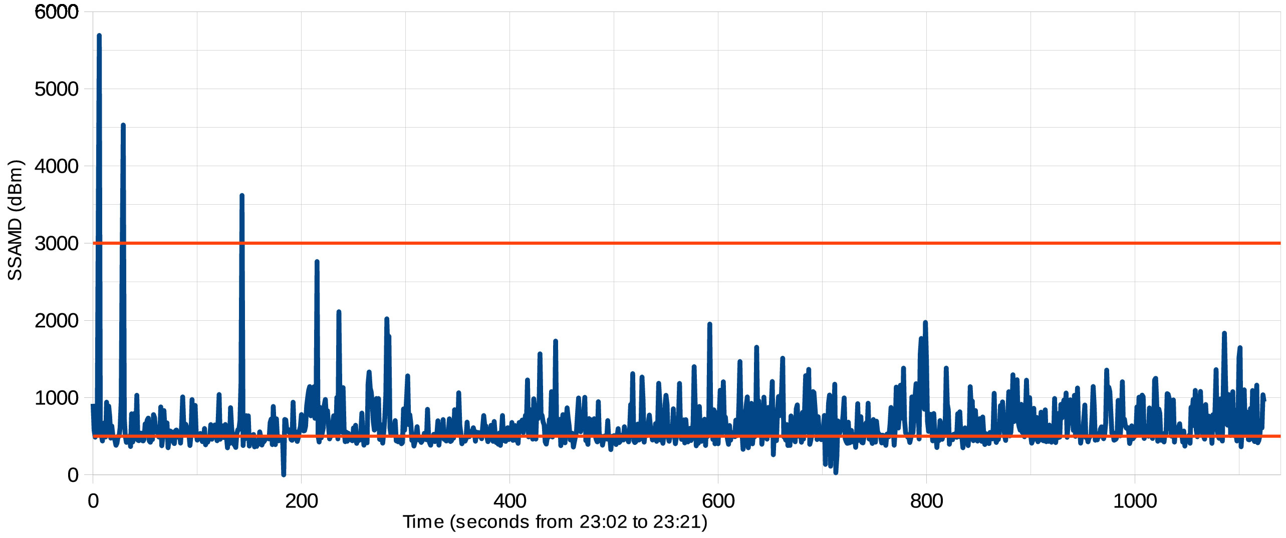
Figure 6 Example of SSAMD measurements on 22 August 2022. The SSAMD insect detection interval is depicted by red lines (500 and 3,000).

Figure 2D illustrates three light trap photos. The first two subfigures from left to right show several insects and correspond to an SSAMD value of approximately 1,000. The last subfigure on the right is associated with an SSAMD value slightly below 500, indicating no insects. Initially, we planned to automatically calculate the number of insects within the radar radiation zone surrounding the light traps’ symmetry axis. However, fieldwork observations have revealed insect behavior’s complexity around the light trap. Insects are often in constant motion, flying and crawling around, making it challenging to count them accurately based on the light trap photos alone.

Furthermore, many insects are not visible to the camera but can be detected by the radar. For example, we frequently observed dynamic flight patterns of hornets and bats that were not captured by the camera but detected by the radar. In situations where multiple insects were attracted to the light trap and suddenly disappeared, bats were likely responsible. Given these complexities, we are exploring alternative approaches that involve working with aggregated values of the number of insects in photos and SSAMD values over a time interval (e.g., 1 h). This can help to filter out unnecessary events and examine the correspondence between aggregated measures (such as average or median) over longer time intervals.

In our previous work (Noskov et al., 2021b), we proposed the concept of a mobile radar mounted on a rover. We showed a mockup setup, demonstrating the feasibility of using a radar unit installed on a rover. Furthermore, we discuss using UGV equipped with radar and other sensors to collect high-resolution spatial forest data.

3.3 Forest reference network for high-accuracy sensor positioning and tree measurements

To ensure accurate positioning in the forest and enable various applications such as UAV time-series adjustment, tree monitoring, and sensor positioning, we deployed a dense reference network in a key forest area covering approximately 5 hectares. This area is already covered by regular UAV RGB point cloud time-series data collected by our colleagues in previous years. The purpose of the dense reference network is to improve the absolute accuracy of the georeferenced data by using equably distributed 3D landmarks, primarily trees.

To establish the reference network, we surveyed during winter when the leaves and vegetation in the forest are minimal, making measurements easier. We began by measuring several basis benchmarks in meadows with excellent GNSS signals. These benchmarks served as reference points with a sub-centimeter absolute accuracy for the XYZ coordinates. In addition, we placed benchmarks within the forest area between the meadows. The winter survey was advantageous as the prism used for measurements remained visible even through dense branches of low trees. The forest benchmarks referenced to the basis benchmarks achieved an accuracy of up to 2 cm, whereas benchmarks defined with other forest benchmarks had an accuracy of approximately 20 cm. Although the 20-cm accuracy is sufficient for UAV data refinement and tree monitoring, we aimed for a centimeter accuracy for sensor (rover) positioning. Consequently, the rover measurements were conducted using benchmarks with the 2-cm accuracy.

All trees in the central part of the key area, totaling 504 trees, were measured using the total station. To measure a tree, the total station was positioned in a location with good visibility of the target tree and access to at least three benchmarks. It was then oriented using the accessible benchmarks, and measurements were taken in reflectorless mode. Two approaches were used for tree measurements: brief and detailed. In the brief mode, a few points along the tree stem were measured, typically including the highest point near the beginning of the crown. This is because the crown can obstruct the direct measurement of the target tree. A detailed mode was employed for a few trees, involving measurements of multiple points along the stem, including all major branches. In some cases, the laser reached the very tip of the branches, allowing for the construction of accurate and detailed 3D tree models. Figure 7 provides an example of a 3D tree model created from the measured points.

FIGURE 7

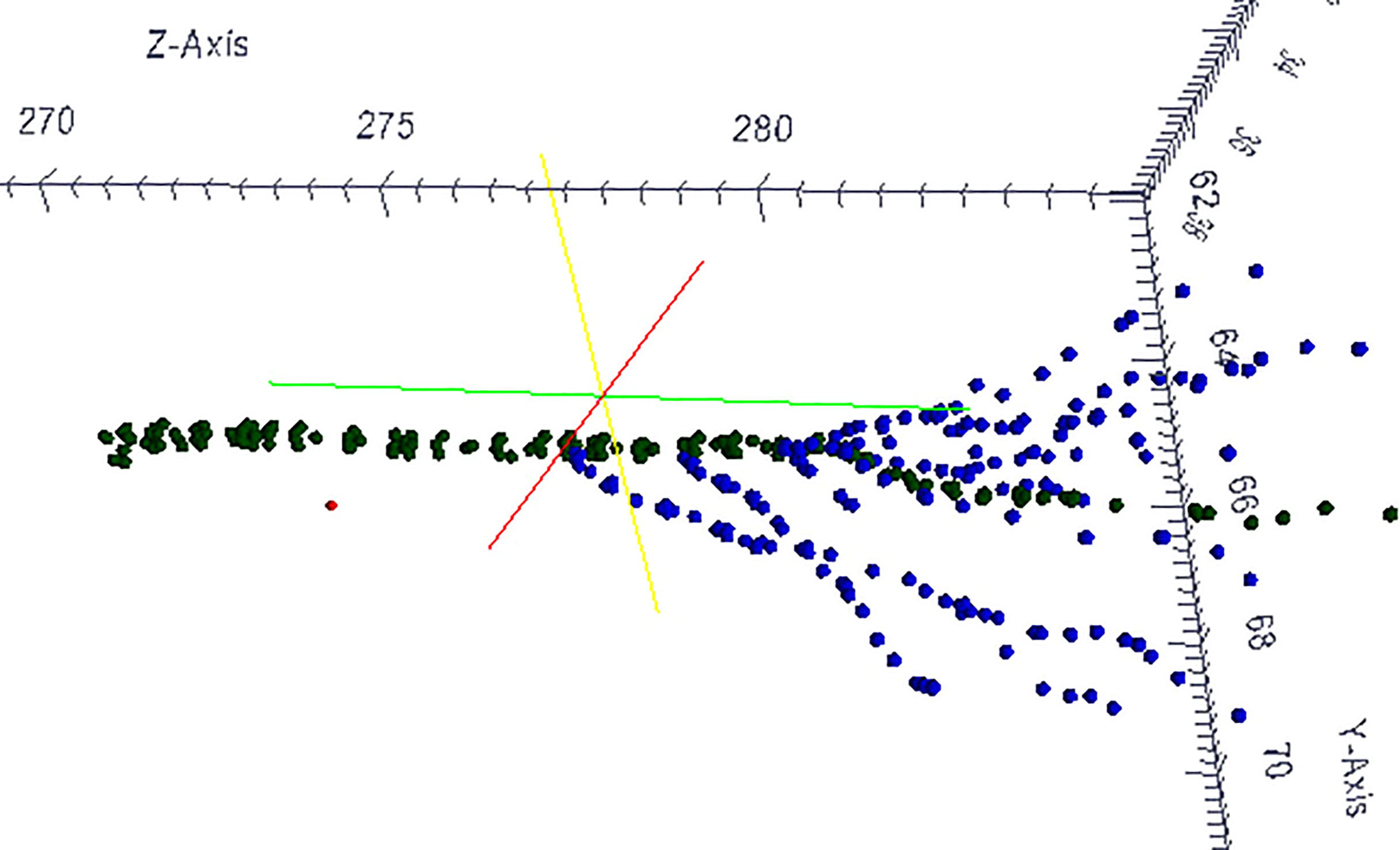
Figure 7 3D model of a tree measured in the detailed mode. Green points, the stem; blue points, the main branches.

The accurate data from the tree measurements are crucial for refining the UAV and multi-sensor rover data. These tree measurements are also essential for interpreting the rover data, as trees are the main objects of interest in the research area. Figure 8 provides an overview of the survey results, including the locations of the original six basis benchmarks in the two meadows, the 28 forest benchmarks distributed within the forest area between the meadows, and the 504 measured trees. These data points collectively contribute to the comprehensive understanding and analysis of the forest ecosystem.

FIGURE 8

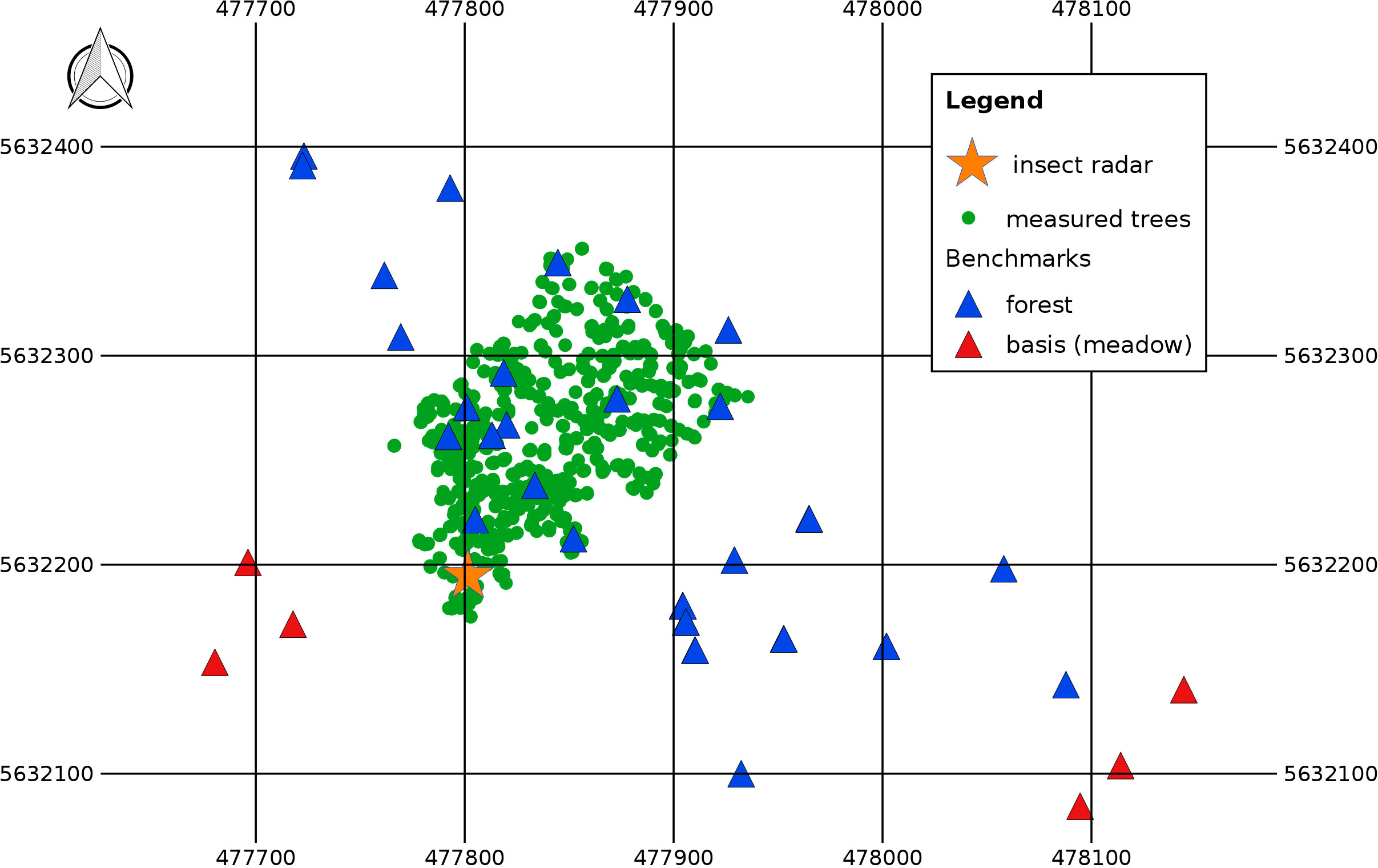
Figure 8 Map of the installed benchmarks and measured trees. Coordinate system: EPSG 32632 (WGS 84/UTM Zone 32N).

3.4 Visually tracked rover workflow and results

The workflow (also earlier sketched in Figure 3B) for conducting fieldwork with the visually tracked rover involves several steps. A single person can handle the equipment and perform the necessary tasks. Here is an overview of the workflow.

3.4.1 Bring the equipment close to the measurement area

The equipment, including the rover, total station, and other necessary tools, is transported near the measurement area.

3.4.2 Install the prism

Attach it to a benchmark and secure it with a pole tripod. This serves as the target for the total station’s tracking.

3.4.3 Setup the total station

Position and orient the total station using accessible benchmarks. Three to six benchmarks are typically used for orientation, ensuring a maximum accuracy of the rover data.

3.4.4 Measure benchmarks

Use the total station to measure the benchmark coordinates, ensuring accurate reference points for positioning.

3.4.5 Prepare the rover

Attach the prism to the rover, ensure time synchronization, and point the total station toward the prism on the rover.

3.4.6 Start tracking mode

Activate the tracking mode on the total station, which records points at regular intervals as the prism moves. A distance interval of 20 cm is typically used to capture the rover’s trajectory.

3.4.7 Drive the rover:

Use a wireless controller to maneuver the rover within the range of the total station. The rover collects data as it moves, capturing detailed information about the forest floor, vegetation, and canopy.

During the fieldwork, the rover’s position coordinates are estimated to have an accuracy of about 2 cm for each coordinate. The total station tracks the prism’s movement, allowing for precise positioning of the rover and ensuring accurate data collection.

The setup and workflow for the visually tracked rover are illustrated in Figure 9, showcasing the process of pointing the total station toward the prism on the rover. The rover can be driven up to a maximum range of approximately 50 m from the total station, enabling extensive coverage of the measurement area.

FIGURE 9

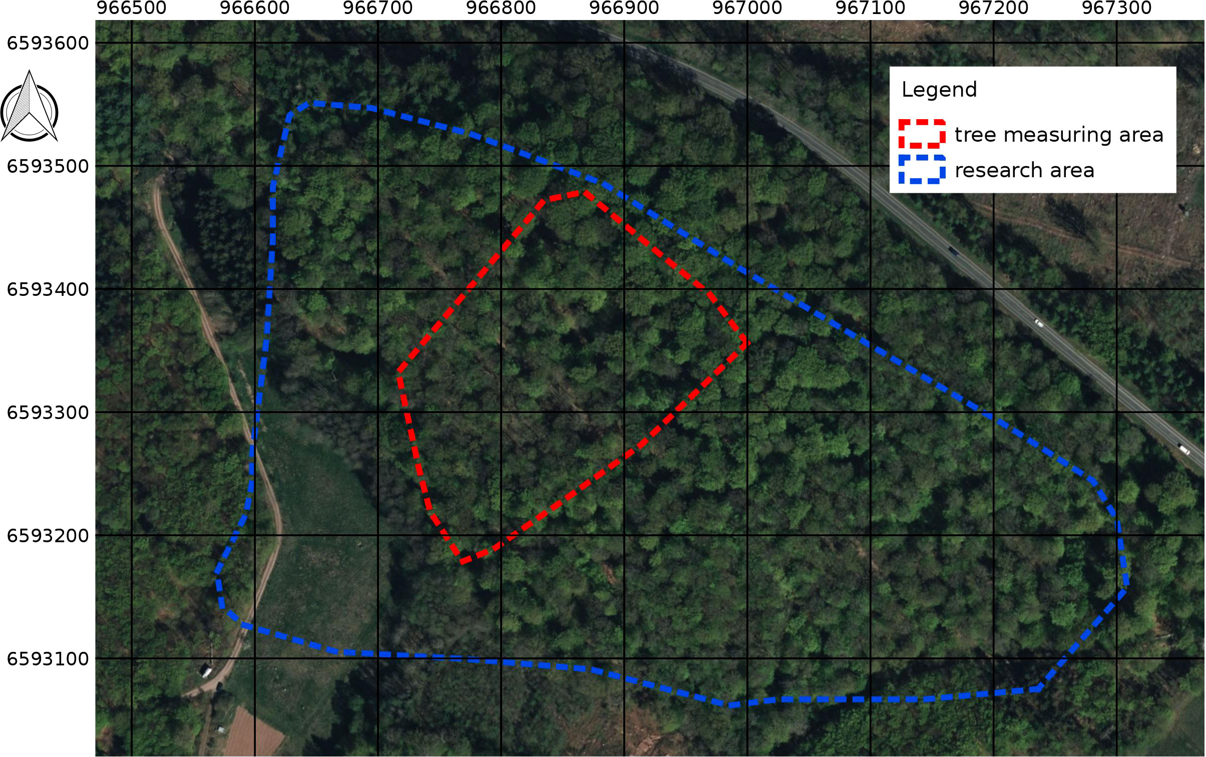
Figure 9 Research area map. Coordinate system: EPSG 32632 (WGS 84 / UTM Zone 32N). Satellite imagery of Bing maps.

Figure 4 depicts the rover prepared for measurements: It is equipped with a prism, powered on, and connected to the wireless controller. The constant blue light on top of the rover in the photo indicates that it is connected and ready to be operated. As previously mentioned, the rover automatically records all data once turned on.

Regarding data collection, the navigation and thematic mapping sensors employ different approaches. The navigation sensors utilize the Robot Operating System (ROS) services to save data in the bag format. Every 6 s, the rover computer initiates writing a new bag file for 2 s. This process captures several RpLidar and front camera frames, along with data from the rover’s internal sensors. On the other hand, the thematic mapping sensors, similar to the insect radar box, record sensor data continuously for the radar and temperature sensors with a 0.02-s pause between data slices.

In addition, the cameras capture photos in a specific sequence. First, the sky-oriented USB camera takes a photo, followed by the ground-oriented NoIR camera. There is then a 2-s break before the process is repeated. The microphone continuously records audio, providing additional information about the workflow. For example, it can detect whether the rover has overturned, which has occurred several times. In the future, the microphone could be used to record bird songs to reconstruct the forest soundscape.

Each photo is time-stamped, allowing for georeferencing using the accurate coordinates of points recorded at short distance intervals from the total station. Prospective plans involve classifying the captured photos using machine learning algorithms to generate high-detail maps of tree crowns and the forest floor.

Figure 10 displays an example of a photo captured by the ground-oriented NoIR camera. It is worth noting that these photos are highly contaminated by infrared radiation. However, as shown in the figure, post-processing techniques can be applied to refine the photos and make them appear more natural. Using a NoIR camera enables nocturnal observations with infrared lighting and the potential for multispectral imaging, such as calculating vegetation indices (Lopez-Ruiz et al., 2017). Although a removable infrared filter can be equipped on the camera, it is not considered necessary as the global shutter front camera captures high-quality, high-resolution RGB photos of the ground surface.

FIGURE 10

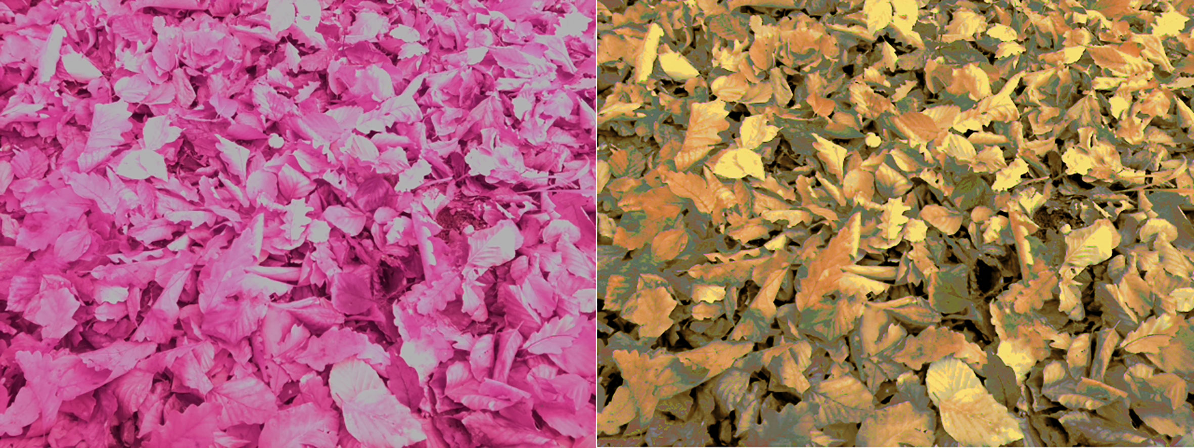
Figure 10 Ground-oriented NoIR camera photo example. Left: original image. Right: processed image with the reduced impact of the infrared radiation [as recommended in (Thomas, 2021)].

Figure 11 illustrates the results obtained from the sample data of sky-oriented sensors, providing an overview of the leaf-fall process. The figure includes photos from the sky-oriented camera and radar SSAMD data. The first subfigure represents a single date, whereas the remaining subfigures represent four different moments in all rounds: 29 October 2022, 15:36:39 (round 1); 3 November 2022, 16:29:28 (round 2); 10 November 2022, 12:41:30 (round 3); and 30 December 2022, 12:22:34 (round 4).

FIGURE 11

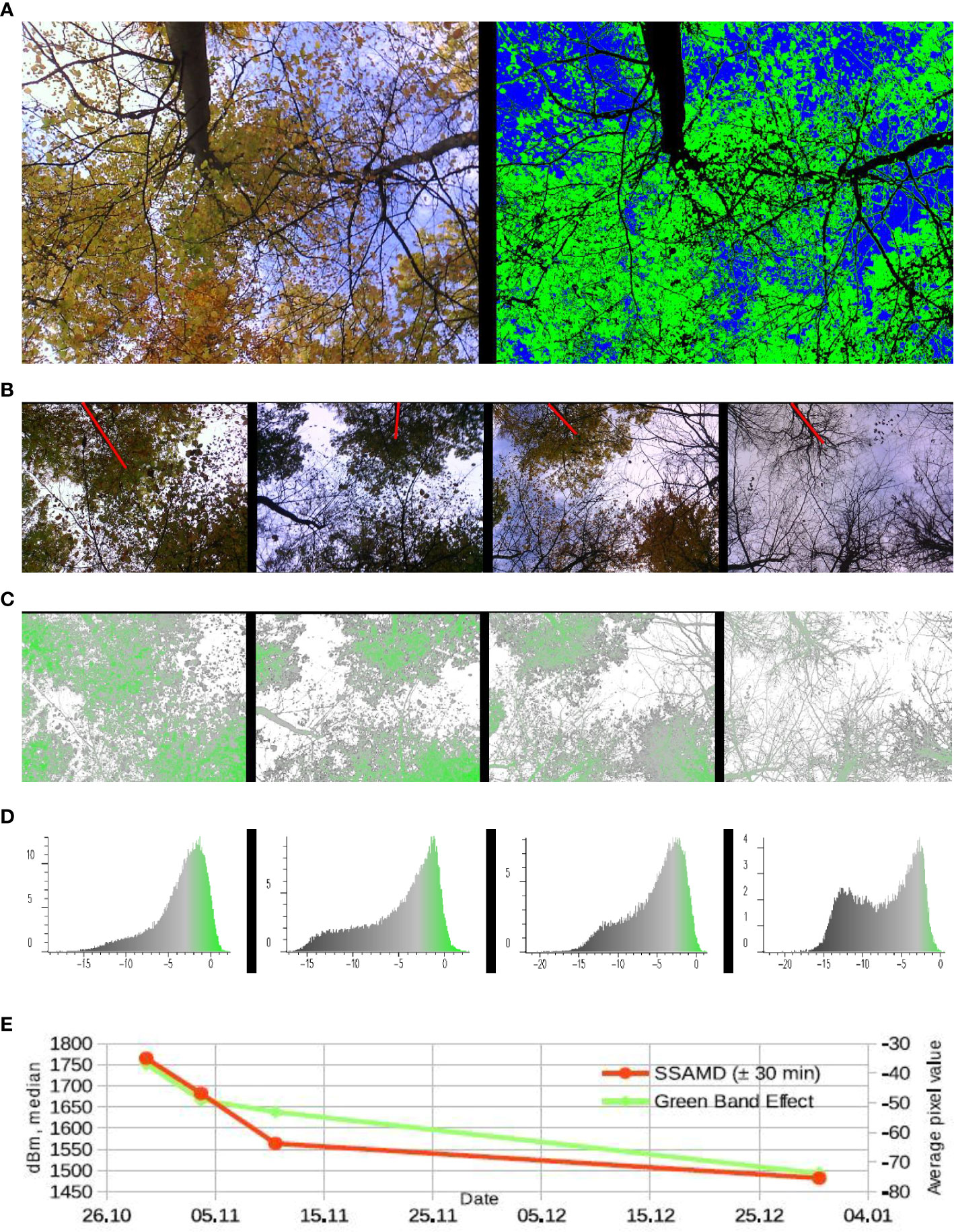
Figure 11 (A) Example of a photo taken by the sky-oriented camera: Left: original image. Right classification results: blue pixels, the sky (ca. 25%); black, tree stems and branches (ca. 25%); and green, leaves (ca. 50%). (B) Sky-oriented photos taken from the same point (coordinate difference within 12 cm) on the following dates (from left to right): 29 October, 3 November, 10 November, and 30 December. Red line indicates the same tree. (C) Green band effect corresponding (see (B)) rasters. The meaning of colors is reflected in (D). (D) Corresponding (see (C)) histograms. X-axis, cell values in tens; Y-axis, number of cells in hundreds. (E) Leaf-fall statistics. Average green band effect and median SSAMD. Leaf-fall observations with the sky-oriented sensors.

Figure 11A presents an example of a photo captured by the sky-oriented camera. This type of data provides valuable insights into the condition of tree crowns. The left subfigure depicts the original photo, whereas the right subfigure displays the result of a classification process. The classification was performed using an unsupervised algorithm, specifically a modified version of the k-means algorithm (Shapiro and GRASS Development Team, 2017). This algorithm classifies the pixels into three distinct groups: leaves, tree stems and branches, and the sky. The classification results enable the calculation of essential statistics for ecological modeling purposes.

Figure 11B displays photos taken from specific points on the corresponding dates. The photos were taken from points with coordinates 477879.35/5632268.82, 477879.37/5632268.93, 477879.32/5632268.85, and 477879.41/5632268.84 (X/Y coordinates in meters of the EPSG 32632 WGS 84 UTM Zone 32N coordinate system). The photos were taken from nearly the same point, with a maximum coordinate difference of less than 12 cm. The following subfigures show the processing results of these photos, including the green band effect and corresponding histograms.

To represent the leaf-fall process using the photos, we propose a simple metric called the “green band effect.” This metric is calculated by subtracting the red and blue channel values from the value of the green channel, with the pixel values ranging from 0 to 255. The green band effect reflects the degree of “greenness” in a specific pixel. We applied unsupervised classification to distinguish sky pixels, which were masked and excluded from subsequent calculations. Figure 11C displays the results of the green band effect calculation, followed by the respective histograms shown in Figure 11D. It is important to note that the same color table is used for the green band effect imagery and the histograms.

Figure 11E presents the aggregated statistics of the green band effect and radar’s SSAMD calculations. The green line represents the dynamics of the average green band effect pixel values, whereas the red line represents the SSAMD calculation. To obtain an aggregated radar reflection of the tree crown conditions, a large time interval of ±30 min from the corresponding photo capture moment is used. Using the median SSAMD allows for reducing the significant effects of shaking, solid and wet obstacles, the operator’s body reflection, and other factors. Both lines show a declining trend, confirming the expected leaf-fall process reflection in the collected data. These statistics demonstrate the promising potential of using the proposed rover concept for measuring crown conditions.

Now, we will showcase examples of maps summarizing the work conducted with the rover thus far, along with the collected temperature information. Given that radar/lidar data and photos entail intensive data processing, our focus has been on surface temperature data. This data source is relatively straightforward and only necessitates a brief workflow description and simple interpretation.

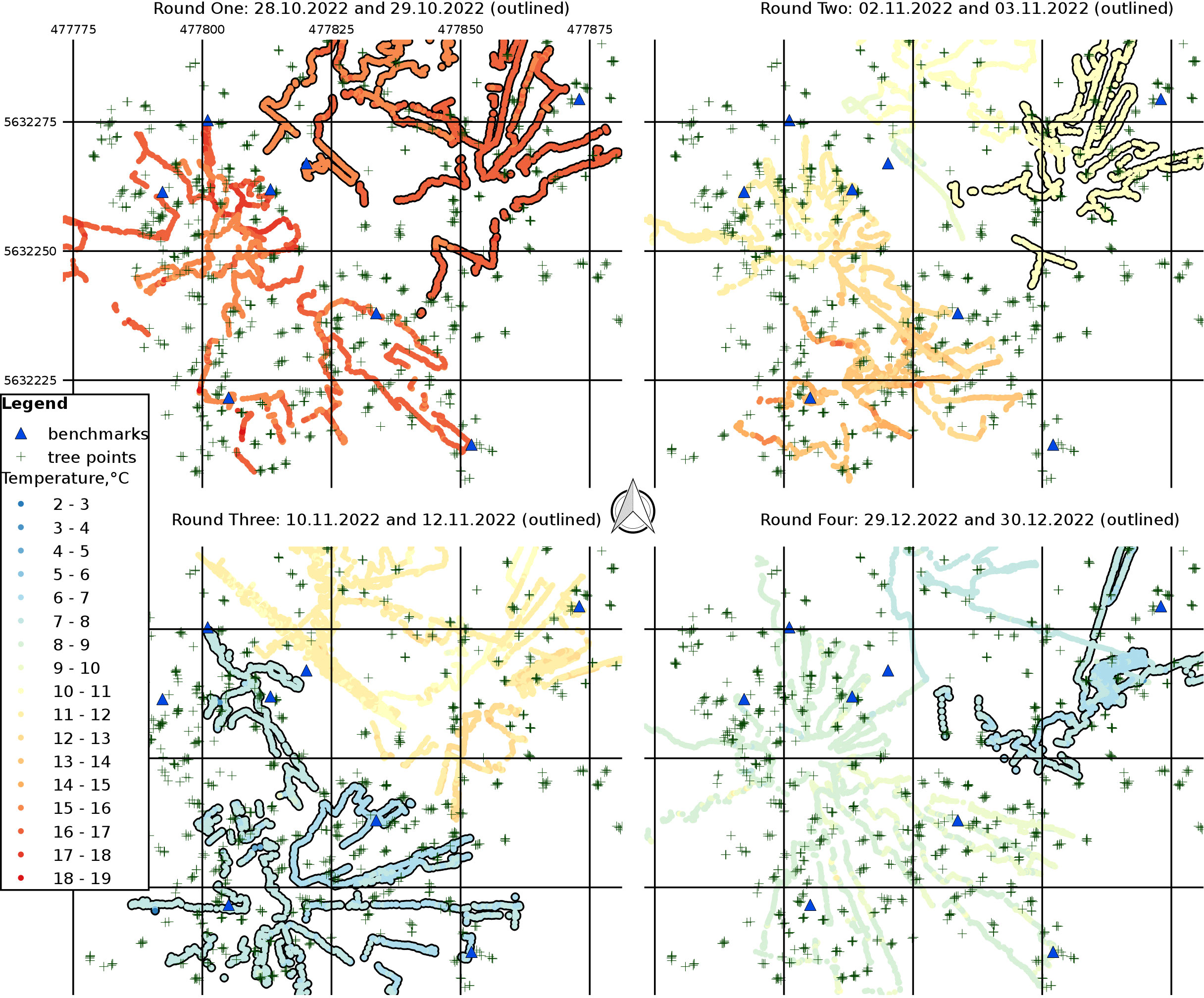
Figure 12 provides an overview of the routes taken by the rover. The rover operator selected the routes intuitively to ensure maximum efficiency in covering the area. The data collection was organized into four rounds, each involving data collection from all planned stations. The figure displays the time at which the points were measured. Each round spanned 2 working days, and the points outlined on the second day of each round are depicted in the figure. The time intervals are represented by color, indicated in hours and minutes (HH : MM format). The maps presented in the figure showcase the routes taken during the four rounds: the first round on 28 and 29 October 2022; the second round on 2 and 3 November 2022; the third round on 10 and 12 November 2022; and the fourth round on 29 and 30 December 2022. These maps illustrate the area covered by the rover routes and the corresponding measurement times.

FIGURE 12

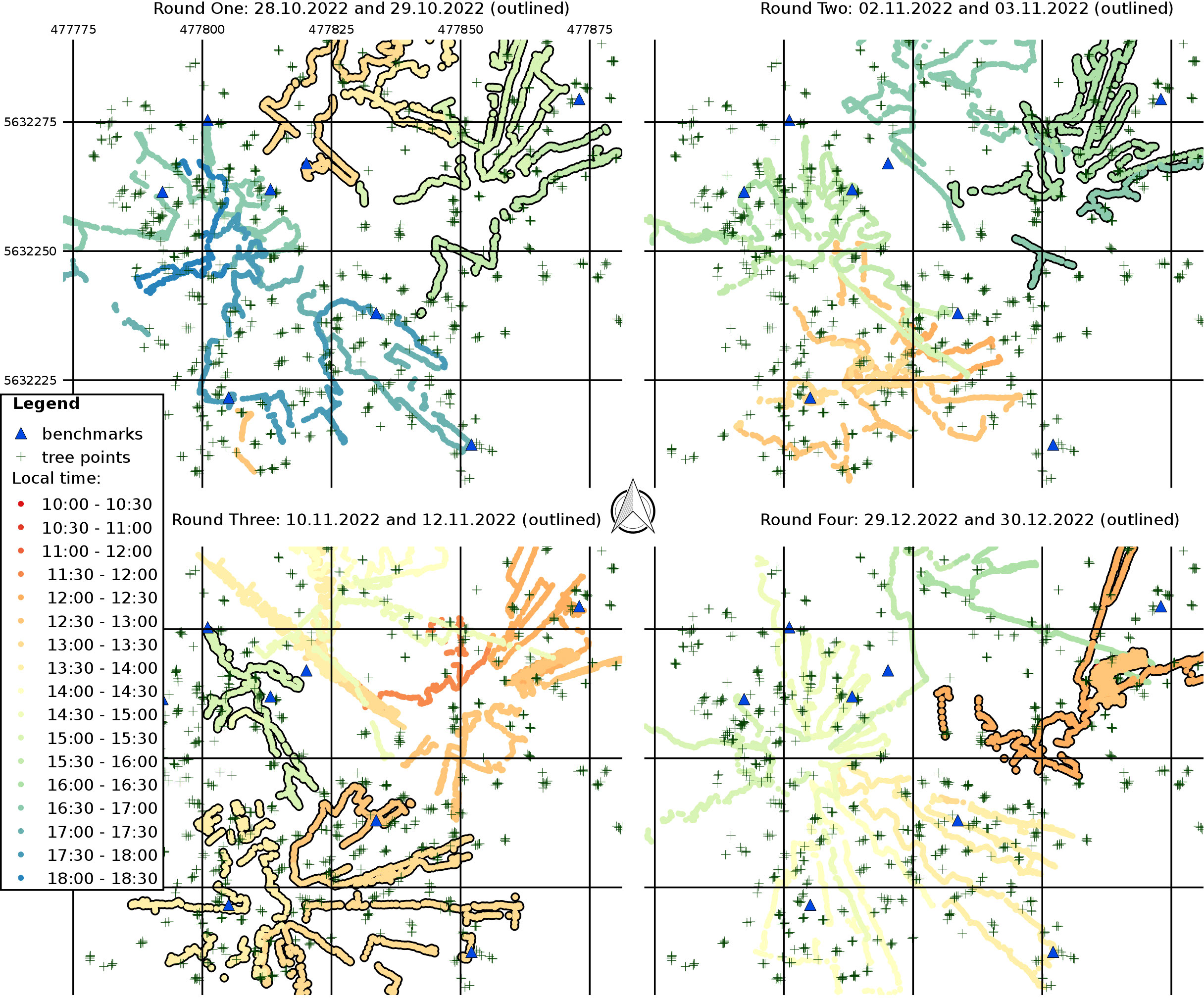
Figure 12 Rover field work routes: Time maps (epoch seconds) of measurements. Coordinate system: EPSG 32632 (WGS 84/UTM Zone 32N).

Figure 13 presents the surface temperature data recorded along the rover routes. The temperature values displayed are the average pixel values captured by the thermal camera, measured in degrees Celsius. The camera’s field of view covers a wide area, with the center point located approximately 1 m behind the rover. In contrast, the infrared thermometer represents a smaller spot on the ground behind the rover, situated in the middle of the NoIR ground-oriented camera’s field of view. The maps clearly illustrate the process of autumn cooling in the forest. It is important to note that the duration of data collection for one round spans 2 working days. As a result, intraday temperature fluctuations significantly impact the recorded data. To ensure accurate modeling of surface temperatures, it is crucial to address and account for these fluctuations in future work carefully.

FIGURE 13

Figure 13 Temperature maps. Coordinate system: EPSG 32632 (WGS 84/UTM Zone 32N).

The demonstrated time and temperature maps confirm the potential to collect highly detailed forest data with a centimeter-level accuracy. Geotagging of the photos taken by the sky- and ground-oriented cameras has already been done using time stamps, and most of the points shown in the time maps have corresponding relevant photos. Adding geotags to the data slices in the ROS *.bag files is also feasible, although it requires more advanced processing due to the point nature of the data captured by these sensors. Because the rover’s orientation influences point data, this can be addressed by calculating the rover’s movement vectors using consecutive position coordinates. Point coordinates can be easily derived by considering the rover’s coordinates and orientation. Different control experiments will be necessary to estimate the accuracy of RpLidar and front camera RGB point coordinates. Furthermore, with knowledge of the rover’s orientation, it becomes possible to convert photos taken by the sky- and ground-oriented cameras into georeferenced imagery, enabling the generation of time series with a centimeter-level accuracy.

4 Conclusions and future work

Recent progress in computers, robotics, and equipment has enabled the development of devices and solutions for high-detail automatic forest monitoring. The introduced devices share common principles.

● They are based on popular open-source compact solutions that enable connecting multiple easily replaceable sensors.

● We propose the autonomous time stamp–based concept for data collecting. It allows the merging of data from various sources.

● Extending the autonomous approach, the presented devices do not require manipulations and configurations for data collecting.

They gather data shortly after powering the devices, facilitating fieldwork, and filtering out irrelevant data.

We have introduced these principles with the proposed compact insect radar box. The conducted fieldwork has shown its effectiveness. Despite the challenging field conditions, we have brought the earlier lab achievements into the forest and collected relatively long and meaningful time series using the radar, camera, and light trap. A preliminary evaluation of these data confirms the effectiveness of the proposed approach. In the next step, we will conduct a detailed analysis of the collected data to research the low nocturnal insect flight. After filtering out the raw data and extracting the insect information, we will use the detailed weather station data to investigate the meteorological factors of the low nocturnal insect flight.

Good progress with the insect radar box has inspired us to more complex solutions. The prepared rover setup has inherited the achievements of the insect radar box. The navigation and multiple thematic sensors work autonomously and separately using time stamps for data merging. The proof-of-concept fieldwork confirmed that our UGV could conduct real measurements in real forest conditions. Several rounds of measurements in the forest have allowed us to collect a large dataset concerning the forest phenology, trees, understory, and forest floor. Several camera sensors, a lidar, a radar, and two thermal sensors facilitate it. The collected data are immediately geotagged using a time stamp. In addition, we have demonstrated the ability to prepare accurate time-series maps. Prospectively, we want to calculate the rover’s orientation for assigning accurate coordinates of the point datasets. Furthermore, it will be likely possible to prepare imagery using sky-, ground-, and front-oriented cameras.

The rover follows a novel principle of visual tracking. It means that the rover is equipped with a prism, and an oriented robotic total station follows this prism automatically and writes position coordinates using a short distance interval. This is one of the earliest attempts to apply a visual tracking rover for monitoring purposes. In future work, we will present the results of the rover data processing and discuss measured forest processes.

We ensure centimeter positioning with the dense reference network in the forest. Several applications require this control network. We have used the network for tree measuring and sensor positioning. Furthermore, we need to increase the accuracy of the distant benchmarks. Moreover, more trees should be measured in the detailed mode.

Data availability statement

The original contributions presented in the study are included in the article/Supplementary Material. Further inquiries can be directed to the corresponding author.

Ethics statement

Written informed consent was obtained from the individual for the publication of any identifiable images or data included in this article.

Author contributions

Conceptualization: AN and JB. Methodology: AN and SA. Software: AN. Validation: AN, SA, and JB. Formal analysis: AN and JB. Investigation: AN, SA, and JB. Resources: AN, SA, and JB. Data curation: AN. Writing—original draft preparation: AN. Writing—review and editing: AN and JB. Visualization: AN. Supervision: JB. Project administration: AN and JB. Funding acquisition: JB. All authors have read and agreed to the published version of the manuscript.

Funding

This research was funded by the Hessian State Ministry for Higher Education, Research and the Arts, Germany, as part of the LOEWE priority project “Nature 4.0-Sensing Biodiversity”. Open Access funding provided by the Open Access Publishing Fund of Philipps-Universität Marburg with support of the Deutsche Forschungsgemeinschaft (DFG, German Research Foundation).

Acknowledgments

Photos shown in Figures 4 and 9 has been taken and prepared by Maik Dobbermann (a technician at Philipps University of Marburg).

Conflict of interest

The authors declare that the research was conducted in the absence of any commercial or financial relationships that could be construed as a potential conflict of interest.

Publisher’s note

All claims expressed in this article are solely those of the authors and do not necessarily represent those of their affiliated organizations, or those of the publisher, the editors and the reviewers. Any product that may be evaluated in this article, or claim that may be made by its manufacturer, is not guaranteed or endorsed by the publisher.

Supplementary material

The Supplementary Material for this article can be found online at: https://www.frontiersin.org/articles/10.3389/fevo.2023.1214419/full#supplementary-material

References

Anastasiou E., Balafoutis A. T., Fountas S. (2023). Trends in remote sensing technologies in olive cultivation. Smart Agric. Technol. 3, 100103. doi: 10.1016/j.atech.2022.100103

CrossRef Full Text | Google Scholar

Arroyo-Rodriguez V., Fahrig L., Tabarelli M., Watling J. I., Tischendorf L., Benchimol M., et al. (2020). Designing optimal human-modified landscapes for forest biodiversity conservation. Ecol. Lett. 23, 1404–1420. doi: 10.1111/ele.13535

PubMed Abstract | CrossRef Full Text | Google Scholar

Barrenetxea G., Ingelrest F., Schaefer G., Vetterli M. (2008). “Wireless sensor networks for environmental monitoring: The sensorscope experience,” in 2008 IEEE International Zurich Seminar on communications, (New York City, United States) 98–101. doi: 10.1109/IZS.2008.4497285

CrossRef Full Text | Google Scholar

Boer M. M., Resco de Dios V., Bradstock R. A. (2020). Unprecedented burn area of Australian mega forest fires. Nat. Climate Change 10, 171–172. doi: 10.1038/s41558-020-0716-1

CrossRef Full Text | Google Scholar

Brach M., Zasada M. (2014). The effect of mounting height on gnss receiver positioning accuracy in forest conditions. Croatian J. For. Eng. 35, 245–253.

Google Scholar

Calders K., Newnham G., Burt A., Murphy S., Raumonen P., Herold M., et al. (2015). Nondestructive estimates of above-ground biomass using terrestrial laser scanning. Methods Ecol. Evol. 6, 198–208. doi: 10.1111/2041-210X.12301

CrossRef Full Text | Google Scholar

Ceccherini G., Duveiller G., Grassi G., Lemoine G., Avitabile V., Pilli R., et al. (2020). Abrupt increase in harvested forest area over europe after 2015. Nature 583, 72–77. doi: 10.1038/s41586-020-2438-y

PubMed Abstract | CrossRef Full Text | Google Scholar

Cook-Patton S. C., Leavitt S. M., Gibbs D., Harris N. L., Lister K., Anderson-Teixeira K. J., et al. (2020). Mapping carbon accumulation potential from global natural forest regrowth. Nature 585, 545–550. doi: 10.1038/s41586-020-2686-x

PubMed Abstract | CrossRef Full Text | Google Scholar

Dataset (2021) Optris CT infrared-thermometer. Available at: https://www.optris.global/optris-ct-lt-ctex-lt (Accessed 1-Feb-2023).

Google Scholar

Dataset (2022) Raspberry Pi camera module 2 NoIR. Available at: https://www.raspberrypi.com/products/pi-noir-camera-v2/ (Accessed 1-Feb-2023).

Google Scholar

Dataset (2023a) Intel RealSense depth camera D435. Available at: https://www.intelrealsense.com/depth-camera-d435/ (Accessed 1-Feb-2023).

Google Scholar

Dataset (2023b) Jackal: unmanned ground vehicle. Available at: https://clearpathrobotics.com/jackal-small-unmanned-ground-vehicle/ (Accessed 1-Feb-2023).

Google Scholar

Dataset (2023c) RpLidar S1: portable TOF laser range scanner. Available at: https://www.slamtec.com/en/Lidar/S1 (Accessed 1-Feb-2023).

Google Scholar

Shaffner T. (2021) MLX90640 thermal camera with Raspberry Pi 4. Available at: https://tomshaffner.github.io/PiThermalCam/ (Accessed 1-Feb-2023). Dataset.

Google Scholar

De Frenne P., Zellweger F., Rodriguez-Sanchez F., Scheffers B. R., Hylander K., Luoto M., et al. (2019). Global buffering of temperatures under forest canopies. Nat. Ecol. Evol. 3, 744–749. doi: 10.1038/s41559-019-0842-1

PubMed Abstract | CrossRef Full Text | Google Scholar

Ellison D., Morris C. E., Locatelli B., Sheil D., Cohen J., Murdiyarso D., et al. (2017). Trees, forests and water: Cool insights for a hot world. Global Environ. Change 43, 51–61. doi: 10.1016/j.gloenvcha.2017.01.002

CrossRef Full Text | Google Scholar

Fahey T. J., Woodbury P. B., Battles J. J., Goodale C. L., Hamburg S. P., Ollinger S. V., et al. (2010). Forest carbon storage: ecology, management, and policy. Front. Ecol. Environ. 8, 245–252. doi: 10.1890/080169

CrossRef Full Text | Google Scholar

Feng T., Chen S., Feng Z., Shen C., Tian Y. (2021). Effects of canopy and multi-epoch observations on single-point positioning errors of a gnss in coniferous and broadleaved forests. Remote Sens. 13. doi: 10.3390/rs13122325

CrossRef Full Text | Google Scholar

Friess N., Bendix J., Brändle M., Brandl R., Dahlke S., Farwig N., et al. (2019). Introducing nature 4.0: A sensor network for environmental monitoring in the marburg open forest. Biodiversity Inf. Sci. Standards 3. doi: 10.3897/biss.3.36389

CrossRef Full Text | Google Scholar

Galiatsatos N., Donoghue D. N., Watt P., Bholanath P., Pickering J., Hansen M. C., et al. (2020). An assessment of global forest change datasets for national forest monitoring and reporting. Remote Sens. 12, 1790. doi: 10.3390/rs12111790

CrossRef Full Text | Google Scholar

Gao Y., Skutsch M., Paneque-Galvez J., Ghilardi A. (2020). Remote sensing of forest degradation: a review. Environ. Res. Lett. 15, 103001. doi: 10.1088/1748-9326/abaad7

CrossRef Full Text | Google Scholar

Ghamry K. A., Kamel M. A., Zhang Y. (2016). “Cooperative forest monitoring and fire detection using a team of uavs-ugvs,” in 2016 International Conference on Unmanned Aircraft Systems (ICUAS). (New York City: IEEE conference proceedings). 1206–1211. doi: 10.1109/ICUAS.2016.7502585

CrossRef Full Text | Google Scholar

Harris N. L., Gibbs D. A., Baccini A., Birdsey R. A., de Bruin S., Farina M., et al. (2021). Global maps of twenty-first century forest carbon fluxes. Nat. Climate Change 11, 234–240. doi: 10.1038/s41558-020-00976-6

CrossRef Full Text | Google Scholar

Huang W., Dolan K., Swatantran A., Johnson K., Tang H., O’Neil-Dunne J., et al. (2019). Highresolution mapping of aboveground biomass for forest carbon monitoring system in the tri-state region of maryland, pennsylvania and delaware, usa. Environ. Res. Lett. 14, 095002. doi: 10.1088/1748-9326/ab2917

CrossRef Full Text | Google Scholar

Hussein M., Renner M., Watanabe M., Iagnemma K. (2013). “Matching of ground-based lidar and aerial image data for mobile robot localization in densely forested environments,” in 2013 IEEE/RSJ International Conference on Intelligent Robots and Systems. (New York City: IEEE conference proceedings). 1432–1437. doi: 10.1109/IROS.2013.6696537

CrossRef Full Text | Google Scholar

Hyyppä E., Yu X., Kaartinen H., Hakala T., Kukko A., Vastaranta M., et al. (2020). Comparison of backpack, handheld, under-canopy uav, and above-canopy uav laser scanning for field reference data collection in boreal forests. Remote Sens. 12. doi: 10.3390/rs12203327

CrossRef Full Text | Google Scholar

Jactel H., Koricheva J., Castagneyrol B. (2019). Responses of forest insect pests to climate change: not so simple. Curr. Opin. Insect Sci. 35, 103–108. doi: 10.1016/j.cois.2019.07.010

PubMed Abstract | CrossRef Full Text | Google Scholar

Lefsky M. A., Cohen W. B., Parker G. G., Harding D. J. (2002). Lidar Remote Sensing for Ecosystem Studies: Lidar, an emerging remote sensing technology that directly measures the threedimensional distribution of plant canopies, can accurately estimate vegetation structural attributes and should be of particular interest to forest, landscape, and global ecologists. BioScience 52, 19–30. doi: 10.1641/0006-3568(2002)052[0019:LRSFES]2.0.CO;2

CrossRef Full Text | Google Scholar

Lopez-Ruiz N., Granados-Ortega F., Carvajal M. A., Martinez-Olmos A. (2017). Portable multispectral imaging system based on raspberry pi. Sensor Rev. 37, 322–329. doi: 10.1108/sr-12-2016-0276

CrossRef Full Text | Google Scholar

Mitchard E. T. A. (2018). The tropical forest carbon cycle and climate change. Nature 559, 527–534. doi: 10.1038/s41586-018-0300-2

PubMed Abstract | CrossRef Full Text | Google Scholar

Nasiri V., Darvishsefat A. A., Arefi H., Pierrot-Deseilligny M., NamIranian M., Le Bris A. (2021). Unmanned aerial vehicles (uav)-based canopy height modeling under leaf-on and leaf-off conditions for determining tree height and crown diameter (case study: Hyrcanian mixed forest). Can. J. For. Res. 51, 962–971. doi: 10.1139/cjfr-2020-0125

CrossRef Full Text | Google Scholar

Nijland W., de Jong R., de Jong S. M., Wulder M. A., Bater C. W., Coops N. C. (2014). Monitoring plant condition and phenology using infrared sensitive consumer grade digital cameras. Agric. For. Meteorology 184, 98–106. doi: 10.1016/j.agrformet.2013.09.007

CrossRef Full Text | Google Scholar

Noskov A. (2021). Low-range FMCW insect radar – lab experiments data, results, and data processing software, (Basel, Switzerland) Dataset. doi: 10.5281/zenodo.5035849

CrossRef Full Text | Google Scholar

Noskov A. (2022). “Radar as a key to global aeroecology,” in Handbook of research on sustainable development goals, climate change, and digitalization, (Basel, Switzerland) 482–505. ch028. doi: 10.4018/978-1-7998-8482-8

CrossRef Full Text | Google Scholar

Noskov A., Achilles S., Bendix J. (2021a). Presence and biomass information extraction from highly uncertain data of an experimental low-range insect radar setup. Diversity 13. doi: 10.3390/d13090452

CrossRef Full Text | Google Scholar

Noskov A., Bendix J., Friess N. (2021b). A review of insect monitoring approaches with special reference to radar techniques. Sensors 21. doi: 10.3390/s21041474

PubMed Abstract | CrossRef Full Text | Google Scholar

Pendrill F., Persson U. M., Godar J., Kastner T. (2019). Deforestation displaced: trade in forest-risk commodities and the prospects for a global forest transition. Environ. Res. Lett. 14, 055003. doi: 10.1088/1748-9326/ab0d41

CrossRef Full Text | Google Scholar

Petrokofsky G., Holmgren P., Brown N. (2011). Reliable forest carbon monitoring – systematic reviews as a tool for validating the knowledge base. Int. Forestry Rev. 13, 56–66. doi: 10.1505/146554811798201161

CrossRef Full Text | Google Scholar

Pugh T. A. M., Lindeskog M., Smith B., Poulter B., Arneth A., Haverd V., et al. (2019). Role of forest regrowth in global carbon sink dynamics. Proc. Natl. Acad. Sci. 116, 4382–4387. doi: 10.1073/pnas.1810512116

CrossRef Full Text | Google Scholar

Qian C., Liu H., Tang J., Chen Y., Kaartinen H., Kukko A., et al. (2017). An integrated gnss/ins/lidarslam positioning method for highly accurate forest stem mapping. Remote Sens. 9. doi: 10.3390/rs9010003

CrossRef Full Text | Google Scholar

Seymour F., Busch J. (2016). Why forests? Why now?: The science, economics, and politics of tropical forests and climate change (Washington DC, United States: Brookings Institution Press).

Google Scholar

Shapiro M., GRASS Development Team (2017). i.cluster module of Geographic Resources Analysis Support System (GRASS) software, version 7.2 (USA: Open Source Geospatial Foundation).

Google Scholar

Tabbush P. (2010). Cultural values of trees, woods and forests (Farnham, Surrey: The Research Agency of the Forestry Commission, UK).

Google Scholar

Taravati S. (2018). Evaluation of low-energy microwaves technology (Termatrac) for detecting western drywood termite in a simulated drywall system. J. Economic Entomology 111, 1323–1329. doi: 10.1093/jee/toy063

CrossRef Full Text | Google Scholar

Thomas (2021) Infrared image processing with gimp. Available at: https://www.fullspectrumuk.com/infrared-image-processing-gimp/ (Accessed 1-Feb-2023). Dataset.

Google Scholar

Vandendaele B., Fournier R. A., Vepakomma U., Pelletier G., Lejeune P., Martin-Ducup O. (2021). Estimation of northern hardwood forest inventory attributes using uav laser scanning (uls): Transferability of laser scanning methods and comparison of automated approaches at the tree- and stand-level. Remote Sens. 13. doi: 10.3390/rs13142796

CrossRef Full Text | Google Scholar

Wallace L., Lucieer A., Watson C., Turner D. (2012). Development of a uav-lidar system with application to forest inventory. Remote Sens. 4, 1519–1543. doi: 10.3390/rs4061519

CrossRef Full Text | Google Scholar

Wear D. N. (2002). The southern forest resource assessment: summary report Vol. 54 (Asheville NC, United States: Southern Research Station).

Google Scholar

Wernick I. K., Ciais P., Fridman J., Hoegberg P., Korhonen K. T., Nordin A., et al. (2021). Quantifying forest change in the european union. Nature 592, E13–E14. doi: 10.1038/s41586-021-03293-w

PubMed Abstract | CrossRef Full Text | Google Scholar

Zhou Y., Williams C. A., Hasler N., Gu H., Kennedy R. (2021). Beyond biomass to carbon fluxes: application and evaluation of a comprehensive forest carbon monitoring system. Environ. Res. Lett. 16, 055026. doi: 10.1088/1748-9326/abf06d

CrossRef Full Text | Google Scholar