A calibration method for SWMM to mitigate the impact of the structure defect without considering runoff on building walls

In this study, we propose a hypothesis that an automatic calibration framework can address modeling uncertainties in the Storm Water Management Model (SWMM) due to structural defects that result in the inability of the model to account for runoff generated on building walls from wind-driven rain. To test this hypothesis, we introduce a rainfall error model into the calibration framework to indirectly consider the effects of inclined wind-driven rain on building walls. We couple the optimization algorithm Differential Evolution Adaptive Metropolis (DREAM) with SWMM using newly developed API functions. To demonstrate the effectiveness of the framework, we conduct a case study in Guangzhou, China and assess the impacts of rainfall uncertainty on model parameter estimations and simulated runoff boundaries. The results show that the framework can improve the average Nash–Sutcliffe index of selected events by more than 5%. It also captures peak flow more accurately. This framework contributes to the theory of SWMM calibration by accounting for structural defects and considering rainfall uncertainty.

Introduction

Urbanization significantly alters hydrological processes and leads to more runoff volume, less concentration time, and more severe flooding (Eakin et al., 2022; Luo et al., 2022; Pallathadka et al., 2022). To analyze and manage the hydrological characteristics of urban watersheds, various urban hydrological models, including the Storm Water Management Model (SWMM), have been developed globally in recent decades (Rodriguez et al., 2008; Rubinato et al., 2013; Bisht et al., 2016). SWMM, an open-source urban hydrological model created by the United States Environmental Protection Agency (US EPA), is widely used in predicting runoff quantity and quality from urban drainage systems. It can simulate both single-event and long-term continuous rainfall–runoff processes in catchments containing different types of gray and/or green infrastructures. However, the SWMM model has a structural limitation as it cannot consider the runoff generated on building walls, leading to a significant influence on the simulation accuracy in certain situations. Raindrops trajectory can tilt under windy conditions, blocking rainfall by building walls and forming runoff on building walls, altering the characteristics of regional runoff generation and concentration significantly (Figure 1) (Blocken and Carmeliet, 2004; Blocken et al., 2013; Gao et al., 2021). Although most studies obscure this wind-effect problem through calibration, ignoring the influence of wind may result in misleading parameter estimates, restricting the application of the SWMM model in designing flooding control facilities and reducing its capacity to predict future responses of flooding events accurately (Hussain et al., 2022; Sytsma et al., 2022).

FIGURE 1

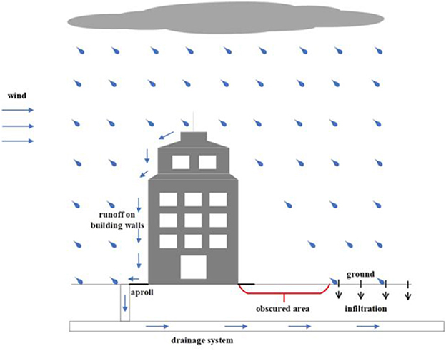
Figure 1. Diagram of the effect of wind on runoff.

Therefore, there is a need to find a way to mitigate modeling uncertainties caused by the structural defect of SWMM. As mentioned earlier, the model structural defect arises from the failure to account for the interaction between inclined rainfall and building walls. As the distribution of building walls remains constant for a given urban area, researchers can reduce the impact of this structural defect by classifying its influence as a part of the rainfall input uncertainty. The objective of this study is to create a calibration framework that can effectively address the issue of rainfall input uncertainty and determine whether it can enhance the robustness of SWMM.

In addition to rainfall input uncertainty, complex hydrological models, such as SWMM, are subject to other types of uncertainties, including equifinality, where multiple parameter sets can produce equally acceptable predictions (Muñoz et al., 2014; Her and Chaubey, 2015; Wagner et al., 2019). To estimate the impact of rainfall input uncertainty and the influence of the previously analyzed structural defect, a calibration method is needed that can distinguish between different types of uncertainties. Several studies have quantified uncertainty in SWMM models, such as Sun et al. (2014), who incorporated the generalized likelihood uncertainty estimation (GLUE) method to analyze parameter uncertainty in a highly urbanized sewershed in Syracuse, NY. Knighton et al. (2016) evaluated the parameter uncertainty of an SWMM model that is developed for the Cathedral Run stormwater wetland using the GLUE method and highlighted the importance of equifinality and uncertainty in stormwater wetland modeling. Raei et al. (2019) developed a framework for low-impact development—best management practices (LID-BMPs) that accounts for parameter uncertainty with a fuzzy α-cut technique. Other studies, such as Sharifan et al. (2010), Zhang and Li (2015), Bellos et al. (2017), and Gorgoglione et al. (2019), have also explored uncertainty analysis in SWMM models. However, most of these studies focus on only one type of uncertainty, highlighting the need for a new calibration framework capable of separating and considering different types of uncertainties.

To address this issue, we employed a Bayesian-based optimal algorithm, namely Differential Evolution Adaptive Metropolis (DREAM), to calibrate the SWMM model. DREAM is an adaptive Markov chain Monte Carlo (MCMC) algorithm that estimates the posterior probability density function of model parameters based on the Bayesian framework. This algorithm is capable of integrating various types of modeling errors into a single likelihood function and estimating their distributions. DREAM was developed by Vrugt et al. (2009) as an adaptation of the Shuffled Complex Evolution Metropolis (SCEM-UA) global optimization algorithm that simultaneously runs multiple chains for global searching and automatically adjusts the scale and orientation of the proposal distribution during evolution to the posterior distribution (Vrugt et al., 2008). DREAM has been shown to be efficient on complex, highly non-linear, and multimodal target distributions while maintaining detailed balance and ergodicity. To enhance the calibration efficiency, we coupled the DREAM method with SWMM by directly exposing the model parameters to the calibration framework using PySWMM, a Python package developed by Emnet (https://github.com/OpenWaterAnalytics/pyswmm). A case study was conducted in Guangzhou, China, to evaluate the effectiveness of this proposed calibration framework in improving the robustness of the SWMM model.

Materials and methods

The SWMM model

SWMM simulates rainfall–runoff process on a collection of sub-catchment areas, which receive precipitation and generate runoff and pollutant loads and transport the generated runoff through a system of pipes, channels, storage/treatment devices, pumps, and regulators (Rossman, 2004). In this study, PySWMM, a Python-packaged version of SWMM 5.1 (https://github.com/OpenWaterAnalytics/pyswmm), was used instead of the original version of SWMM 5.1. PySWMM is free software developed by Emnet. It provides a Python interface for SWMM. With PySWMM, users can control the functions and objects in SWMM through Python and develop algorithms exclusively in Python to control the calculation process of SWMM. Some API functions are developed and added into the model to obtain and adjust parameter values, such as impervious rate and maximum infiltration rate of a sub-catchment in the SWMM model, while the model is running. With these API functions, the automatic calibration algorithm and the SWMM model can be connected easily through a Python platform. A rainfall error model used to describe the rainfall input uncertainty, which will be illustrated below in detail, is also integrated into the SWMM model to consider rainfall uncertainty.

SWMM model calibration

For prediction purposes, the parameter values should accurately reflect the invariant properties of the specific system that they represent (Vrugt et al., 2008). However, although most of the parameters in the SWMM model have physical meanings, there are some parameters, which cannot be measured directly. Therefore, these parameters need to be meaningfully derived through calibration against historical records of some state quantities of the catchment.

The hydrological simulation of a catchment by the SWMM model can be expressed by Eq. (1):

$\begin{array}{ll}Y=f(\theta ,\widehat{\zeta },\widehat{\varphi }),& (1)\end{array}$

where Y = {y₁, …, y_n} represents the simulated results of the model such as streamflow; $\widehat{\zeta }$ refers to the measured boundary such as precipitation and evapotranspiration; $\widehat{\varphi }$ represents the initial conditions; θ = {θ₁, …, θ_d} represents model parameters; and f represents the deterministic or stochastic transition function (the SWMM model in this study). Let Ŷ = {ŷ₁, …, ŷ_n} represent measurements of observed system behavior (streamflow in this study). The difference between Y and Ŷ can be mathematically expressed by the residual vector [Eq. (2)]:

$\begin{array}{ll}{\epsilon }_i\left(\theta |\widehat{Y},\widehat{\zeta },\widehat{\varphi }\right)=y_i\left(\theta |\widehat{\zeta },\widehat{\varphi }\right)-{\widehat{y}}_{i}i=1,\dots ,n.& (2)\end{array}$

The calibration is to make the residuals as close as zero. The traditional approach is to build an objective function for the residuals, such as the sum of squared residuals [which is shown in Eq. (3)], and to minimize the objective function by tuning the values of the parameters.

$\begin{array}{ll}SSR\left(\theta |\widehat{Y},\widehat{\zeta },\widehat{\varphi }\right)={\displaystyle \sum _{i=1}^n{\epsilon }_i{\left(\theta |\widehat{Y},\widehat{\zeta },\widehat{\varphi }\right)}^2}.& (3)\end{array}$

The approach mentioned above only focuses on errors caused by the model parameters but ignores the errors associated with model inputs, initial conditions, model structures, and measurements of observed system behavior (streamflow in this paper). Therefore, it may not obtain the “best-fit” values of the parameters or obtain fake “best-fit” parameters that do not represent the properties of the real-world hydrologic system. Physically, the errors associated with initial conditions can be eliminated with the model running. As the model input, such as precipitation and evapotranspiration, is of high spatio-temporal heterogeneity, the errors associated with the model input are much greater than that associated with streamflow measurements. Consequently, the residual vector between Y and Ŷ can be rewritten as Eq. (4):

$\begin{array}{ll}{\epsilon }_i\left(\theta ,s\left(\widehat{\zeta }\right)|\widehat{Y},\widehat{\varphi }\right)=y_i\left(\theta ,s\left(\widehat{\zeta }\right)|\widehat{\varphi }\right)-{\widehat{y}}_i\text{ }i=1,\dots ,n,& (4)\end{array}$

where s represents the error function of the model input.

An algorithm, which can consider different sources of error, is needed to minimize the residuals expressed in Eq. (4). Bayesian statistics coupled with Monte Carlo sampling is a practical method to settle this problem (Vrugt et al., 2009). It can estimate different sources of errors simultaneously and give the posterior distribution of the parameters of the SWMM model and the input errors model. Assuming that the residuals described in Eq. (4) are independent and Gaussian distributed with constant variance (σ_e) and a constant mean (0), the posterior probability density function of the parameters, including parameters of the SWMM model and the input errors model, can be identified as follows:

$\begin{array}{l}p\left(\theta ,s\left(\widehat{\zeta }\right)|\widehat{Y},\widehat{\varphi }\right)\\ =c·p\left(\theta \right)·p\left(s\left(\widehat{\zeta }\right)\right)\\ {\displaystyle \prod _{i=1}^n\frac{1}{\sqrt{2\pi {\sigma }_e}}\exp \left(-\frac{{\left(y_i\left(\theta ,s\left(\widehat{\zeta }\right)|\widehat{\varphi }\right)-{\widehat{y}}_i\right)}^2}{2{\sigma }_e^2}\right)},& (5)\end{array}$

where c is a normalizing contact; and p(θ) and $p(s(\widehat{\zeta }))$ represent the prior distribution of θ and $s(\widehat{\zeta })$, respectively.

However, the assumption of the independent identical distribution of the residuals is usually not realistic in hydrologic modeling. The time series of residuals are typically autocorrelated and non-stationary. To obtain relatively reasonable parameters and predictive uncertainty, a first-order autoregressive (AR) scheme of the residuals is introduced [Eq. (6)]. The first-order AR model can at least partly account for the autocorrelation of residuals and thus the influence of model structural uncertainty.

$\begin{array}{ll}{\epsilon }_i=\rho {\epsilon }_{i-1}+v_{i}i=1,\cdots ,n,& (6)\end{array}$

where ρ is the first-order correlation coefficient, ε_i is the residual (ε₀ = 0), and $v~N(0,{{\sigma }_v}^2)$ is the unexplained error and Gaussian-distributed with constant variance (σ_v) and a constant mean (0). With the AR-1 model shown in Eq. (6), the residual time series can be represented by

$\begin{array}{l}{\delta }_i\left(\theta ,s\left(\widehat{\zeta }\right),\rho |\widehat{Y},\widehat{\varphi }\right)={\epsilon }_i\left(\theta ,s\left(\widehat{\zeta }\right)|\widehat{Y},\widehat{\varphi }\right)\\ -\rho {\epsilon }_{i-1}\left(\theta ,s\left(\widehat{\zeta }\right)|\widehat{Y},\widehat{\varphi }\right).& (7)\end{array}$

The posterior probabilities of the parameters can then be identified as follows:

$\begin{array}{l}p\left(\theta ,s\left(\widehat{\zeta }\right),\rho |\widehat{Y},\widehat{\varphi }\right)=c·p\left(\theta \right)·p\left(s\left(\widehat{\zeta }\right)\right)·p\left(\rho \right)\\ {\displaystyle {\prod }_{i=1}^n\frac{1}{\sqrt{2\pi {\sigma }_v}}\exp \left(\text{}-\frac{{\delta }_i{(\text{}\theta ,s\left(\text{}\widehat{\zeta }\text{}\right),\rho |\widehat{Y},\widehat{\varphi }\text{})}^2}{2{\sigma }_v^2}\right).}& (8)\end{array}$

As the probability distribution defined in Eq. (8) cannot be derived through analytical analysis, a newly developed MCMC method called DREAM was introduced to generate samples from the posterior probability distribution. In calibration, σ_v was also regarded as a calibration parameter.

To reduce heteroscedasticity, the observed and simulated streamflow is transformed by the BOX-COX method (Box and Cox, 1964):

$\begin{array}{ll}\tau (Y,\lambda )=\{\begin{array}{cc}(Y^{\lambda }-1)/\lambda & if\lambda \ne 0\\ \ln (Y)& if\lambda =0\end{array}& (9)\end{array}$

where Y represents the observed and simulated streamflow and λ is a transformation parameter and can be obtained by maximum-likelihood estimation.

Input error of the model

The storm depth multiplier model (Kavetski et al., 2003) is chosen to consider the uncertainty associated with rainfall forcing. The model introduces a multiplier for each rainfall event based on the idea that the rainfall depth measurements may have a systematic error for each storm caused by the movement of the storm cell within the catchment, but the internal storm pattern may be kept relatively well (Kavetski et al., 2006). By tuning these multipliers (m = {m₁, …, m_n}) within a reasonable range, the errors associated with rainfall forcing can be reduced. Compared with the additive errors model, the multiplicative errors model has an advantage that it does not depend on the scale of rainfall depths while it cannot correct observed rainfall depths of zero (Kavetski et al., 2006; Vrugt et al., 2008).

Generally, the multipliers are assumed to be subject to a Gaussian distribution with the variance (σ_m) and a constant mean (μ_m). Based on the assumption that rain gauges tend to capture unbiased rainfall depths, μ_m was set to 1. As to how to obtain the value of σ_m, please refer to Kavetski et al. (2006) for details. In this study, σ_m was estimated jointly with other parameters through the proposed calibration framework.

Substitute the input error model in Eq. (8) with the storm depth multiplier model, Eq. (8) changes to

$\begin{array}{l}p\left(\theta ,m,\rho |\widehat{Y},\widehat{\varphi }\right)=c·p\left(\theta \right)·p\left(\rho \right)·N\left(m|{\mu }_m,{\sigma }_m^2\right)\\ {\displaystyle {\prod }_{i=1}^n\frac{1}{\sqrt{2\pi {\sigma }_v}}\exp \left(\text{}-\frac{{\delta }_i{\left(\theta ,s\left(\widehat{\zeta }\right),\rho |\widehat{Y},\widehat{\varphi }\right)}^2}{2{\sigma }_v^2}\right)}.& (10)\end{array}$

Distributed routing effect algorithm for mobility

Distributed Routing Effect Algorithm for Mobility is an adaptive MCMC algorithm to efficiently estimate the posterior probability density function of parameters in high-dimensional, complex sampling problems (Vrugt et al., 2009). The method explores global optimal samples by running multiple chains simultaneously and tuning the scale and orientation of the proposal distribution to the posterior distribution automatically. The method shows excellent efficiency on multimodal target, highly non-linear, and complex distributions while maintaining ergodicity and detailed balance.

The linkage between DREAM and SWMM

DREAM and the SWMM model were connected within a Python platform. As described in Section The SWMM model, the SWMM model was packaged through Python language, and some APIs used to obtain and change the parameter values of the SWMM model were developed and added to the model. With the APIs, the DREAM method can obtain and adjust the model parameters directly instead of rewriting the input file of the SWMM model frequently, which can improve the efficiency of computation. Besides, the storm depth multiplier (m) was integrated into the SWMM model to consider the rainfall input uncertainty. The calibration procedure is as follows (Figure 2):

Step 1. The parameters of the integrated model, combining the SWMM model, AR-1 model, and storm depth multiplier model, are sampled through the DREAM module according to their prior probability distributions. If rainfall uncertainty is not considered, the values of all the storm depth multipliers will be set to 1.

Step 2. The sampled parameter values are passed to the integrated model through the developed APIs. The streamflow is then simulated by the model, and the posterior probabilities are calculated based on the simulated and observed streamflow.

Step 3. The Markov chain is expanded through the DREAM algorithm according to the obtained posterior probabilities. The termination condition of the Markov chain is then checked. If the termination condition is met, stop the calibration, otherwise, return to Step 1.

FIGURE 2

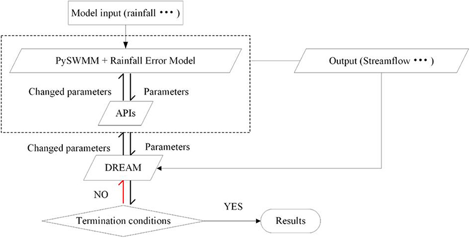
Figure 2. The structure and workflow of the developed calibration framework.

The workflow of different calibration frameworks (with and without the storm depth multiplier model) is similar. The multipliers of the storm depth multiplier model are sampled in the framework considering the rainfall uncertainty but set to be 1 in the framework not considering the rainfall uncertainty model.

Study area and model building

Study area and data collection

For the application study, a small commercial area located in Zhihuicheng, Guangzhou, China was selected. Zhihuicheng is situated in the northeast of the Tianhe district of Guangzhou, characterized by a subtropical monsoon climate with an average annual precipitation of 1,650 mm and an annual mean temperature of 21.8°C. The area experiences heavy rainfall from April to September, which causes frequent flooding. With relatively flat terrain, the study area spans 11.37 hm², with commercial land accounting for approximately 70% of the land use. Figure 3 provides detailed information on the study area, including its main features.

FIGURE 3

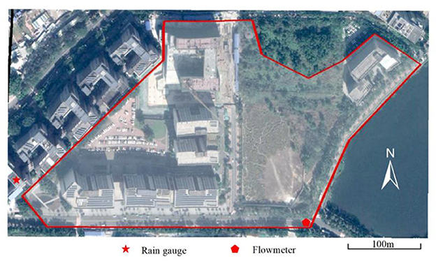
Figure 3. Map of the study area and locations of monitoring equipment. The area within the red line is the study area. Map data: © Google, Maxar Technologies.

Rainfall data were collected using a self-recorded tipping rain gauge placed on the roof of the tallest building located southwest of the study area, with an accuracy of 0.2 mm. Runoff data were collected using an ultrasonic flowmeter with an accuracy of 2% FS, placed in the manhole near the outfall of the drainage system of the area, with a collection interval of 1 min. The rain gauge and flowmeter were manufactured by THWater (http://www.thuenv.com/h-col-103.html), with their specific locations shown in Figure 3.

Eight rainfall events and the corresponding streamflow were selected for the case study. The details of the rainfall events are shown in Table 1.

TABLE 1

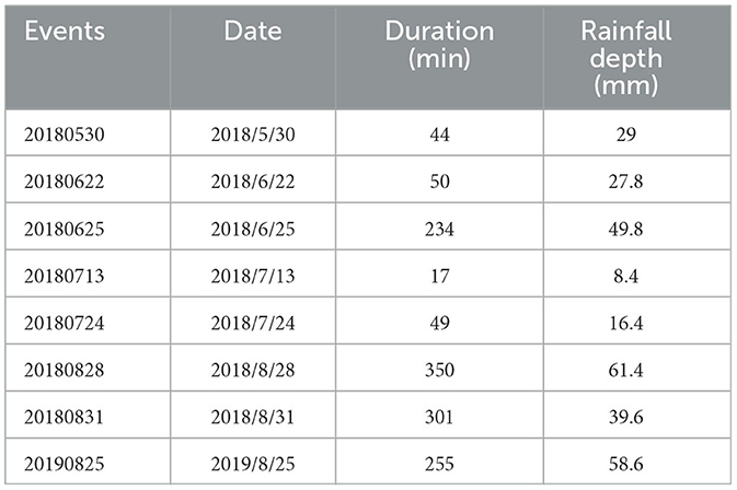
Table 1. Details of the rainfall events.

Model building

The study area was divided into 34 sub-catchments based on the topography and distribution of manholes. The drainage system consisted of 29 junctions (each representing a manhole), 30 conduits, and 1 outfall, as obtained from the local government and verified through field investigation. The land use data and soil type were also obtained through field investigation, with commercial land being the predominant land use and clay being the primary soil type.

To model the infiltration process, the Green-Ampt method was employed, while the dynamic wave method, a complete solution of the one-dimensional Saint-Venant flow equation, was used to model the routing process. SWMM provides various infiltration and routing methods, but these two methods were chosen for this study. The spatial distribution of the drainage system and sub-catchments is shown in Figure 4.

FIGURE 4

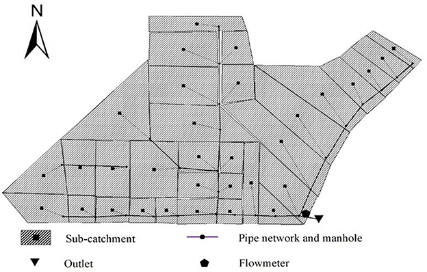
Figure 4. Watershed overview in the SWMM model.

Parameter sensitivity analysis

To reduce the number of parameters considered during calibration, sensitivity analysis is usually performed beforehand to distinguish influential from non-influential parameters. In this study, the Morris method (Niazi et al., 2017; Behrouz et al., 2020) was utilized for the parameter sensitivity analysis, which identifies global sensitivity by sampling local derivatives on a specific grid throughout the parameter space. Nine parameters were identified as sensitive in the study area, including “width,” which was represented by Eq. (11) to maintain the spatial variation of the parameter while reducing the dimension of the parameter set. The details of these parameters are shown in Table 2.

TABLE 2

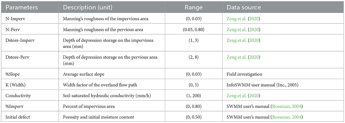
Table 2. Value range of the sensitive parameter.

Based on the sensitivity analysis, the study identifies nine parameters that are considered sensitive within the study area. To reduce the parameter set's dimension while retaining the “width” parameter's spatial variation across different sub-catchments, the parameter “width” is represented by Eq. (11) Table 2 shows the details of these parameters. Although the modeling results are highly sensitive to the percentage of impervious surfaces, the study did not choose it as a calibration parameter. This is because it is a measurable parameter and is not influenced by the modeling scale.

$\begin{array}{ll}W=K·\sqrt{A},& (11)\end{array}$

Where W represents the width of the sub-catchment; A represents the area of the corresponding sub-catchment; and K is a scale factor that needs to be calibrated.

Calibration strategy

To calibrate the model, the first six rainfall events and their corresponding streamflow at the outfall were used for calibration, while the last two rainfall events and their corresponding streamflow were used for verification. Two calibration approaches were employed to evaluate the impact of rainfall input uncertainty, and thus, partly the wind effect, on model calibration: one with a storm depth multiplier model and one without.

All parameters, except for the “width” parameter, were assumed to be the same across different sub-catchments due to the relatively small and simple study area, where these parameters vary little. The “width” parameter, represented by “K”, varied between sub-catchments of different shapes. After the Markov chains converge (Vrugt et al., 2009), a total of twice the number of calibrated parameters Markov chains were obtained, and the last one-third of the samples in each chain were used to summarize the marginal densities of parameters and generate simulated outputs. It should be noted that, unlike the first calibration approach, which resulted in unrealistic values for some parameters due to compensating for errors in rainfall data, the posterior marginal probability density distributions of all parameters calibrated using the second approach, which considers both parameter uncertainty and input uncertainty, were approximately Gaussian, indicating that the optimal values of all parameters were located in physically reasonable ranges.

The residuals, the peak streamflow bias, and the total streamflow bias were selected as the calibration objectives. The Nash–Sutcliffe index (E_NS), the peak flow bias, and the total streamflow bias were used to evaluate the calibration efficiency, which are shown in Eq. (12–14).

$\begin{array}{ll}{E}_{NS}=1-\frac{{\displaystyle {\sum }_{t=1}^n{(q_{t,obs}-q_{t,sim})}^2}}{{\displaystyle {\sum }_{t=1}^n{(q_{t,obs}-\overline{q_{obs}})}^2}}& (12)\end{array}$

$\begin{array}{ll}{E}_{QW}=\frac{{\displaystyle {\sum }_{t=1}^n(q_{t,obs}-q_{t,sim})}}{{\displaystyle {\sum }_{t=1}^n{q}_{t,obs}}}& (13)\end{array}$

$\begin{array}{ll}{E}_{PR}=\frac{q_{p,obs}-q_{p,sim}}{q_{p,obs}}& (14)\end{array}$

where q_{t, obs} and q_{t, sim} represent the observed streamflow and simulated streamflow, respectively; q_{p, obs} and q_{p, sim} represent the observed peak flow and simulated peakflow, respectively; $\overline{q_{obs}}$ represents the average of the observed streamflow; t represents the time step of the streamflow sequence; and n represents the total number of the runoff sequence.

Results and discussion

The estimation of model parameters was initially conducted by considering only the parameter uncertainty. Figure 5 shows the posterior marginal probability density distributions of the estimated parameters. The results demonstrate that the estimations of K, %Imperv for commercial land, %Imperv for green land, and Dstore-Imperv are primarily located in a relatively narrow interval, which is within the individual prior range of the parameters. This suggests that these parameters are more sensitive in the study area than others and that the DREAM method can identify reasonable parameter values. However, it should be noted that most parameters are approximately Gaussian, except for %Imperv for commercial land, %Imperv for green land, and N-imperv. The posterior marginal probability distributions of these parameters are significantly different from the normal distribution, with most probability mass concentrated at the upper boundaries of these parameters. This indicates that the optimal parameter values may fall beyond the physically realistic range. The contradiction between the optimal parameter values and the physical limitations could be attributed to the representativeness of the parameter itself, the structural deficiencies of SWMM, and the errors in the input data.

FIGURE 5

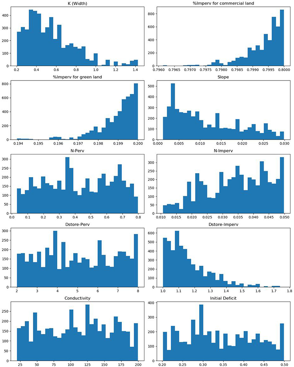
Figure 5. The posterior marginal probability density distributions of parameters only considering parameter uncertainty.

Figure 6 presents a comparison between the simulated and observed runoff of the outfall, while Figure 7 displays the Nash–Sutcliffe indices of the simulations. Overall, the calibrated SWMM model can well capture the fluctuation characteristics of the runoff for most rainfall events, as shown by the Nash–Sutcliffe indices that exceed 0.55 for the majority of the events, except for event 20180831. However, the relatively low Nash–Sutcliffe index for this event is due to the significant underestimation of the streamflow after the peak flow. This could be caused by measurement errors in runoff or domestic sewage discharged into the drainage system, given the absence of rainfall during this period.

FIGURE 6

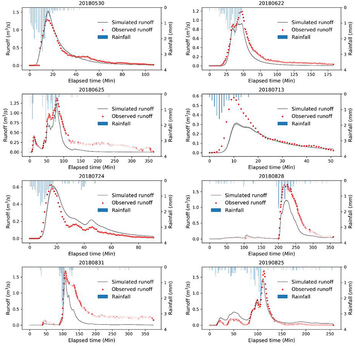
Figure 6. Comparison between the observed runoff and simulated runoff using the model calibrated only considering parameter uncertainty. The shadow of the black line represents the 95% uncertainty range caused by parameter uncertainty.

FIGURE 7

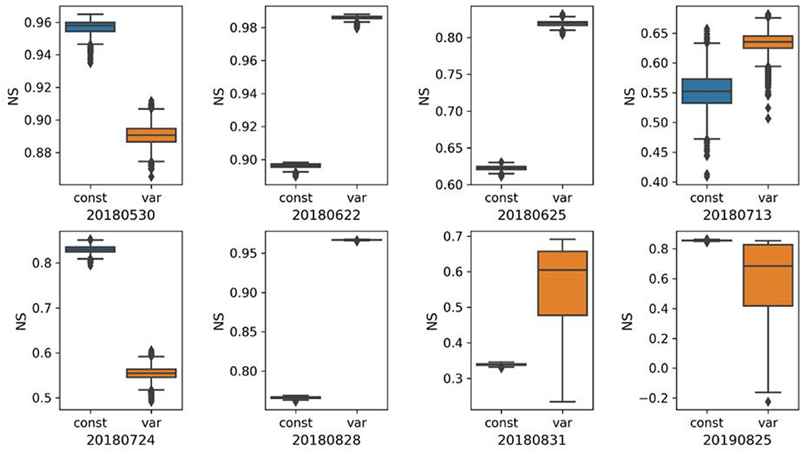
Figure 7. Comparison of Nash–Sutcliffe indices of the simulations obtained through the two different calibration approaches. “const” and “var” refer to calibration strategies that do not consider and consider input uncertainties, respectively. The boxes indicate the 25th, 50th, and 75th percentiles of the scaling rates, and the vertical lines indicate the 5th and 95th percentiles. Black markers refer to values >1.5 times the interquartile range away from the bottom or top of the box.

Furthermore, the hydrographs of the simulated runoff in Figure 6 reveal that the uncertainty of the simulated runoff is not as significant as that suggested by the posterior marginal probability distributions of the model parameters. In other words, the uncertainty of the parameters is greater than that of the simulated runoff, indicating that different parameter sets could lead to similar simulated results. This confirms the presence of equifinality in the SWMM model. It is also worth noting that the calibrated SWMM model tends to underestimate the peak flow for most rainfall events. This suggests that flood control facilities designed solely based on the SWMM model calibrated considering only parameter uncertainty may fail to perform adequately.

Figure 8 shows the posterior marginal probability density distributions of the selected model parameters and storm depth multipliers obtained from the calibration considering both parameter and input uncertainty. In contrast to the distributions obtained from calibration only considering parameter uncertainty, the distributions of all parameters are approximately Gaussian, indicating that the optimal parameter values are within physically realistic ranges. The differences between the two calibration approaches suggest that the unrealistic parameter values for %Imperv of commercial and green land and N-imperv obtained from the first approach were likely to compensate for errors in the rainfall data.

FIGURE 8

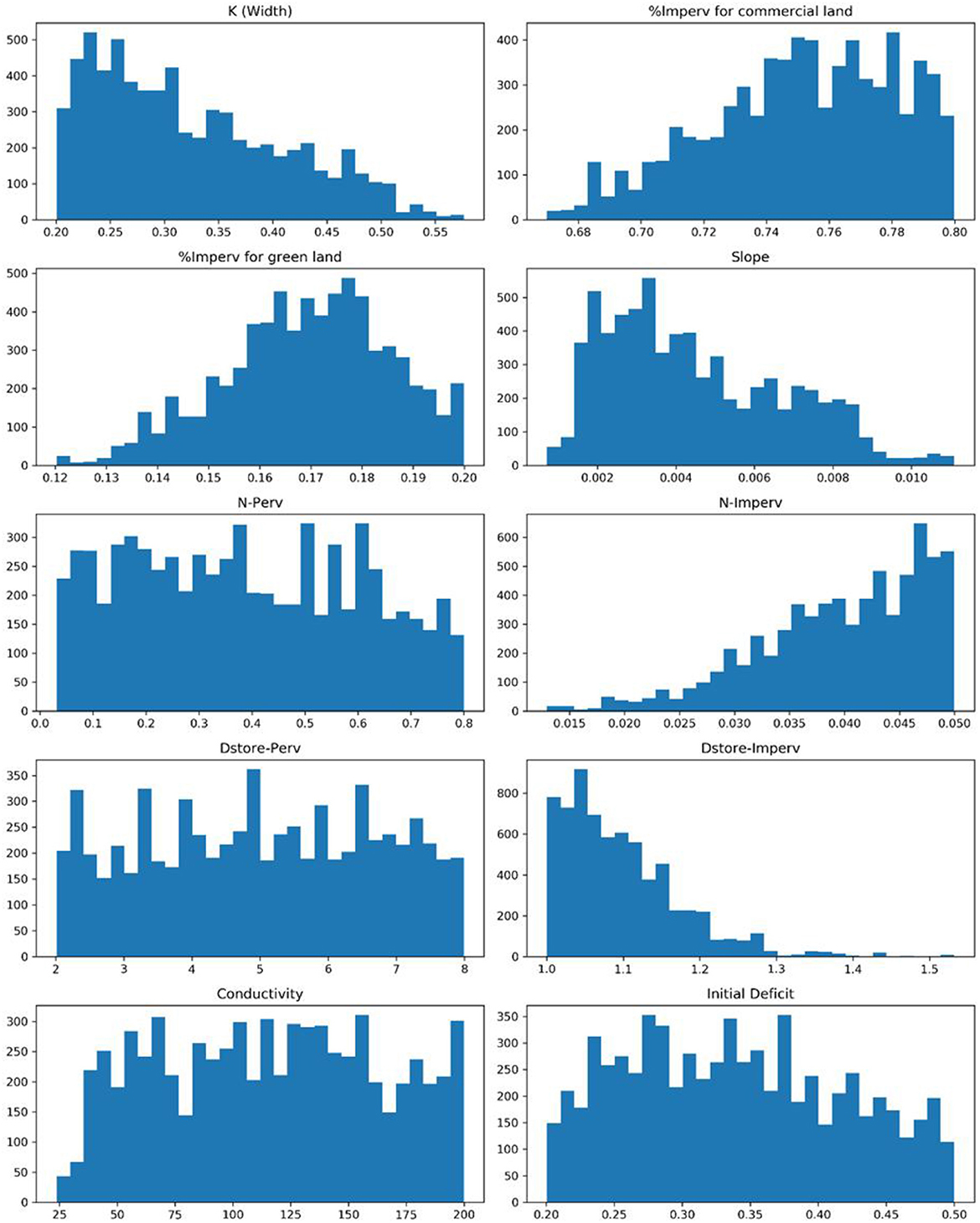
Figure 8. The posterior marginal probability density distributions of parameters calibrated considering both parameter uncertainty and input uncertainty.

In Figure 9, additional contrast is presented for parameter values derived from the two calibration methods. The findings indicate that, with the exclusion of the N-Perv parameter, the majority of parameter values exhibit a notable distinction between the two calibration methods. The reason for the exemption of the N-Perv parameter could be due to the insignificant effect that this parameter has on the simulated runoff in the study region, as the ratio of permeable surfaces in the study locality is relatively low.

FIGURE 9

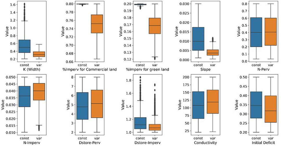
Figure 9. Comparison of parameter values obtained from the two different calibration approaches. The boxes indicate the 25th, 50th, and 75th percentiles of the scaling rates, and the vertical lines indicate the 5th and 95th percentiles. Black markers refer to values >1.5 times the interquartile range away from the bottom or top of the box.

Figure 10 displays the posterior marginal probability density distributions of storm depth multipliers, indicating that most of the storm depth multipliers are approximately Gaussian distributed, except for the storm depth multipliers of rainfall events during the validation period. This result suggests that the DREAM method can effectively define storm depth multipliers. It should be noted that the storm depth multipliers during the validation period were randomly sampled from the storm depth multiplier samples of rainfall events during the calibration period, which may have caused the abnormal distributions of the storm depth multipliers during the validation period.

FIGURE 10

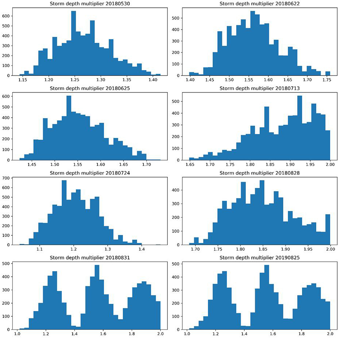
Figure 10. The posterior marginal probability density distributions of storm depth multipliers.

From Figure 11, it is evident that the medians of storm depth multiplier samples range from 1.2 to 2.0 in the study area, indicating that the rain gauge underestimates the actual rainfall depth significantly. This result contradicts the findings of Vrugt et al. (2008), who observed that most storm depth multipliers are distributed around 1 in their study on input uncertainty in hydrological modeling of natural watersheds. It has been suggested in some studies that precipitation data obtained by tipping bucket rain gauges can be largely influenced by the wind field nearby (Dotto et al., 2014).

FIGURE 11

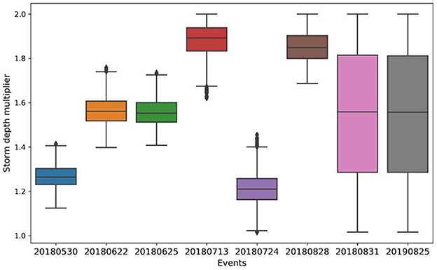
Figure 11. Comparison of storm depth multipliers for different rainfall events. The boxes indicate the 25th, 50th, and 75th percentiles of the scaling rates, and the vertical lines indicate the 5th and 95th percentiles. Black markers refer to values >1.5 times the interquartile range away from the bottom or top of the box.

To investigate the relationship between storm depth multipliers and nearby wind fields, we present the corresponding wind speeds of the rainfall events in Table 3. The results reveal that higher wind speeds are generally associated with greater storm depth multipliers, indicating that the wind field has a significant impact on rainfall errors. Notably, the underestimation of rainfall depth in our study is more severe than in other studies. This may be attributed to the placement of the rainfall gauge on the roof of a building, where turbulence is intensified by the wind-blocking effect of the building, thereby significantly reducing the catch efficiency of rainfall gauges. While antecedent soil moisture is another factor that can influence storm depth multipliers, it is expected to have a relatively small effect in the studied area due to the predominance of impervious surfaces.

TABLE 3

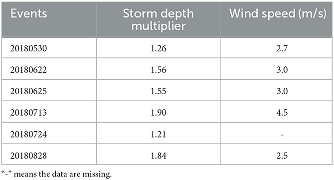
Table 3. Wind speeds corresponding to the studied rainfall events.

Figure 12 shows the comparison between the simulated runoff, which considers both parameter and input uncertainties, and the observed runoff used as the reference. The results indicate that the approach that considers both parameter and input uncertainties produces better peak flow predictions than the approach that only considers parameter uncertainty, especially during the validation period. This suggests that the former approach is more appropriate for runoff prediction, which serves as the basis for designing urban flood control facilities. Nash–Sutcliffe indices of runoff simulations obtained through the two calibration approaches are compared in Figure 6. Most of the Nash–Sutcliffe indices of simulations obtained from the model calibrated considering both parameter and input uncertainties are greater than those obtained from the model calibrated only considering parameter uncertainty. Although the Nash–Sutcliffe indices of runoff simulations considering both parameter and input uncertainty are less than that only considering parameter uncertainties for events 20180530 and 20180724, they are still acceptable. Furthermore, the optimal model parameter values calibrated considering both parameter and input uncertainties are more physically realistic than those calibrated only considering parameter uncertainty. These results suggest that the calibration approach considering both parameter and input uncertainties is more robust than that only considering parameter uncertainty. Moreover, the discharge of 20180831 is underestimated by both calibration strategies. It may be caused by the SWMM models that do not consider society's water cycle, as the underestimation occurs during the peak period for domestic sewage discharge.

FIGURE 12

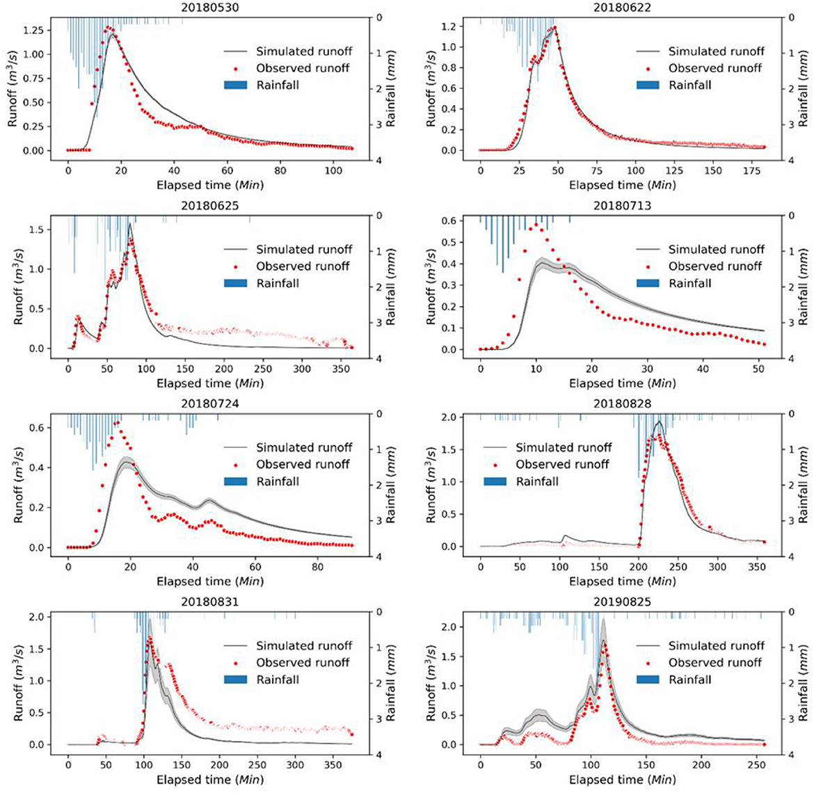
Figure 12. Comparison between the observed runoff and simulated runoff using the model calibrated considering both parameter uncertainty and input uncertainty. The shadow of the black line represents the 95% uncertainty range caused by parameter uncertainty and input uncertainty.

Although the case study shows that the proposed framework can mitigate the impact of the structural defect to some extent. it should be noted that the framework only solves the problem from a data perspective. It cannot distinguish the specific impact of the model structural defects and lead to more uncertainties in simulated results. In a further study, the runoff on building walls should be considered in a more physical way.

Conclusion

In this study, an automatic calibration framework, which can mitigate modeling uncertainties arising from the structural defect of SWMM, was developed based on Bayesian theory. The framework considered both parameter and rainfall uncertainties and integrated DREAM and modified SWMM through newly developed API functions in SWMM to obtain and adjust parameter values. Additionally, a rainfall error model featuring a storm depth multiplier was incorporated to account for systematic errors and partially consider the wind effect. A case study in Guangzhou, China, was conducted to demonstrate the use of the calibration framework. The calibration capability of the framework was tested, and the impacts of rainfall uncertainty on model parameter estimations and simulated runoff boundaries were identified. The main conclusions are as follows.

(1) The contradiction between the optimal parameter values and the physical limitations is probably ascribed to the representativeness of the parameter itself, the structural deficiencies of SWMM, and the errors in the input data. The newly developed framework can obtain relatively reasonable parameter values of SWMM models. (2) The rain gauge tends to underestimate the actual rainfall depth obviously in the study area and ignoring rainfall uncertainty may lead to unrealistic estimations of model parameters. (3) Higher wind speed leads to a greater storm depth multiplier, indicating that the effect of the wind field is an important source of rainfall errors. Parameter values estimated when considering both parameter uncertainty and rainfall uncertainty are well defined within their physically realistic ranges in the study area. (4) Calibration considering both parameter uncertainty and rainfall uncertainty captures peak flows much better and is more robust in terms of the Nash–Sutcliffe index than that only considering parameter uncertainty.

In conclusion, this study offers a reliable approach to improving the accuracy of SWMM through an automatic calibration framework that accounts for uncertainties in model parameters and rainfall.

Data availability statement

The datasets presented in this study can be found in online repositories. The names of the repository/repositories and accession number(s) can be found in the article/supplementary material.

Author contributions

XG, ZX, and JZ: conceptualization. XG: methodology, software, and visualization. CM, ZX, JZ, YM, and XG: validation. CM: formal analysis, investigation, and writing—original draft preparation. JZ and XG: resources and funding acquisition. CM and XG: data curation. JZ and ZX: writing—review and editing. XG, ZX, YM, and JZ: supervision and project administration. All authors have read and agreed to the published version of the manuscript.

Funding

This research was funded by the China Postdoctoral Science Foundation (Grant Number 2022M713472), the Open Research Fund of State Key Laboratory of Simulation and Regulation of Water Cycle in River Basin, China Institute of Water Resources and Hydropower Research (Grant Number IWHR-SKL-202105), and China Three Gorges Corporation Research Project (Contract Nos: 202103429 and 202203050).

Acknowledgments

The authors would like to express their appreciation to the editor and the reviewers, who provided very helpful comments to improve the manuscript.

Conflict of interest

ZX was employed by the company China Three Gorges Corporation.

The authors declare that this study received funding from China Three Gorges Corporation Research Project (Contract No: 202103429; 202203050). The funder had the following involvement in the study: design, collection.

Publisher's note

All claims expressed in this article are solely those of the authors and do not necessarily represent those of their affiliated organizations, or those of the publisher, the editors and the reviewers. Any product that may be evaluated in this article, or claim that may be made by its manufacturer, is not guaranteed or endorsed by the publisher.

References

Behrouz, M. S., Zhu, Z., Matott, L. S., and Rabideau, A. J. (2020). A new tool for automatic calibration of the storm water management model (SWMM). J. Hydrol. 581, 124436. doi: 10.1016/j.jhydrol.2019.124436

CrossRef Full Text | Google Scholar

Bellos, V., Kourtis, I. M., Moreno-Rodenas, A., and Tsihrintzis, V. A. (2017). Quantifying roughness coefficient uncertainty in urban flooding simulations through a simplified methodology. Water 9, 944. doi: 10.3390/w9120944

CrossRef Full Text | Google Scholar

Bisht, D. S., Chatterjee, C., Kalakoti, S., Upadhyay, P., Sahoo, M., and Panda, A. (2016). Modeling urban floods and drainage using SWMM and MIKE URBAN: a case study. Nat. Hazards 84, 749–776. doi: 10.1007/s11069-016-2455-1

CrossRef Full Text | Google Scholar

Blocken, B., and Carmeliet, J. (2004). A review of wind-driven rain research in building science. J. Wind. Eng. Ind. Aerodyn. 92, 1079–1130. doi: 10.1016/j.jweia.2004.06.003

CrossRef Full Text | Google Scholar

Blocken, B., Derome, D., and Carmeliet, J. (2013). Rainwater runoff from building facades: a review. Build Environ. 60, 339–361. doi: 10.1016/j.buildenv.2012.10.008

CrossRef Full Text | Google Scholar

Box, G. E., and Cox, D. R. (1964). An analysis of transformations. J. R. Stat. Soc., B: Stat. Methodol. 26, 211–243. doi: 10.1111/j.2517-6161.1964.tb00553.x

CrossRef Full Text | Google Scholar

Dotto, C. B. S., Kleidorfer, M., Deletic, A., Raush, W., and McCarthy, D. T. (2014). Impacts of measured data uncertainty on urban stormwater models. J. Hydrol. 508, 28–42. doi: 10.1016/j.jhydrol.2013.10.025

CrossRef Full Text | Google Scholar

Eakin, H. C., Parajuli, J., Hernández Aguilar, B., and Yogya, Y. (2022). Attending to the social–political dimensions of urban flooding in decision-support research: A synthesis of contemporary empirical cases. Wiley Interdiscip. Rev. Clim. Chan. 13, e743. doi: 10.1002/wcc.743

CrossRef Full Text | Google Scholar

Gao, X., Yang, Z., Han, D., Gao, K., and Zhu, Q. (2021). The impact of wind on the rainfall–runoff relationship in urban high-rise building areas. Hydrol. Earth Syst. Sci. 25, 6023–6039. doi: 10.5194/hess-25-6023-2021

CrossRef Full Text | Google Scholar

Gorgoglione, A., Bombardelli, F. A., Pitton, B. J., Oki, L. R., Haver, D. L., and Young, T. M. (2019). Uncertainty in the parameterization of sediment build-up and wash-off processes in the simulation of sediment transport in urban areas. Environ. Model. Softw. 111, 170–181. doi: 10.1016/j.envsoft.2018.09.022

CrossRef Full Text | Google Scholar

Her, Y., and Chaubey, I. (2015). Impact of the numbers of observations and calibration parameters on equifinality, model performance, and output and parameter uncertainty. Hydrol. Process 29, 4220–4237. doi: 10.1002/hyp.10487

CrossRef Full Text | Google Scholar

Hussain, S. N., Zwain, H. M., and Nile, B. K. (2022). Modeling the effects of land-use and climate change on the performance of stormwater sewer system using SWMM simulation: case study. J. Water Clim. Chang. 13, 125–138. doi: 10.2166/wcc.2021.180

CrossRef Full Text | Google Scholar

Kavetski, D., Franks, S. W., and Kuczera, G. (2003). Confronting input uncertainty in environmental modelling. Calibrat. Watershed Models 6, 49–68. doi: 10.1029/WS006p0049

CrossRef Full Text | Google Scholar

Kavetski, D., Kuczera, G., and Franks, S. W. (2006). Bayesian analysis of input uncertainty in hydrological modeling: 1. Theory.Water Resour. Res. 42. doi: 10.1029/2005WR004368

PubMed Abstract | CrossRef Full Text | Google Scholar

Knighton, J., Lennon, E., Bastidas, L., and White, E. (2016). Stormwater detention system parameter sensitivity and uncertainty analysis using SWMM. J. Hydrol. Eng. 21, 05016014. doi: 10.1061/(ASCE)HE.1943-5584.0001382

PubMed Abstract | CrossRef Full Text | Google Scholar

Luo, P., Luo, M., Li, F., Qi, X., Huo, A., Wang, Z., et al. (2022). Urban flood numerical simulation: research, methods and future perspectives. Environ. Model. Softw. 105478. doi: 10.1016/j.envsoft.2022.105478

CrossRef Full Text | Google Scholar

Muñoz, E., Rivera, D., Vergara, F., Tume, P., and Arum,í, J. L. (2014). Identifiability analysis: towards constrained equifinality and reduced uncertainty in a conceptual model. Hydrol. Sci. J. 59, 1690–1703. doi: 10.1080/02626667.2014.892205

CrossRef Full Text | Google Scholar

Niazi, M., Nietch, C., Maghrebi, M., Jackson, N., Bennett, B. R., Tryby, M., et al. (2017). Storm water management model: Performance review and gap analysis. J. Sustain. Water Built Environ. 3, 04017002. doi: 10.1061/JSWBAY.0000817

PubMed Abstract | CrossRef Full Text | Google Scholar

Pallathadka, A., Sauer, J., Chang, H., and Grimm, N. B. (2022). Urban flood risk and green infrastructure: who is exposed to risk and who benefits from investment? A case study of three US Cities. Lands. Urban Plan. 223, 104417. doi: 10.1016/j.landurbplan.2022.104417

CrossRef Full Text | Google Scholar

Raei, E., Alizadeh, M. R., Nikoo, M. R., and Adamowski, J. (2019). Multi-objective decision-making for green infrastructure planning (LID-BMPs) in urban storm water management under uncertainty. J. Hydrol. 579, 124091. doi: 10.1016/J.jhydrol.2019.124091

CrossRef Full Text | Google Scholar

Rodriguez, F., Andrieu, H., and Morena, F. (2008). A distributed hydrological model for urbanized areas–model development and application to case studies. J. Hydrol. 351, 268–287. doi: 10.1016/j.jhydrol.2007.12.007

CrossRef Full Text | Google Scholar

Rossman, L. A. (2004). Storm Water Management Model User's Manual, Version 5.0. Cincinnati, OH: National Risk Management Research Laboratory, Office of Research and Development, US Environmental Protection Agency.

Google Scholar

Rubinato, M., Shucksmith, J., Saul, A. J., and Shepherd, W. (2013). Comparison between InfoWorks hydraulic results and a physical model of an urban drainage system. Water Sci. Technol. 68, 372–379. doi: 10.2166/wst.2013.254

PubMed Abstract | CrossRef Full Text | Google Scholar

Sharifan, R. A., Roshan, A., Aflatoni, M., Jahedi, A., and Zolghadr, M. (2010). Uncertainty and sensitivity analysis of SWMM model in computation of manhole water depth and subcatchment peak flood. Procedia-Soc. Behav. Sci. 2, 7739–7740. doi: 10.1016/j.sbspro.2010.05.205

CrossRef Full Text | Google Scholar

Sun, N., Hong, B., and Hall, M. (2014). Assessment of the SWMM model uncertainties within the generalized likelihood uncertainty estimation (GLUE) framework for a high-resolution urban sewershed. Hydrol. Process 28, 3018–3034. doi: 10.1002/hyp.9869

CrossRef Full Text | Google Scholar

Sytsma, A., Crompton, O., Panos, C., Thompson, S., and Mathias Kondolf, G. (2022). Quantifying the uncertainty created by non-transferable model calibrations across climate and land cover scenarios: a case study with SWMM. Water Resour. Res. 58, e2021WR031603. doi: 10.1029/2021WR031603

CrossRef Full Text | Google Scholar

Vrugt, J. A., Ter Braak, C. J., Clark, M. P., Hyman, J. M., and Robinson, B. A. (2008). Treatment of input uncertainty in hydrologic modeling: doing hydrology backward with Markov chain Monte Carlo simulation. Water Resour. Res. 44, W00B09. doi: 10.1029/2007WR006720

CrossRef Full Text | Google Scholar

Vrugt, J. A., Ter Braak, C. J., Gupta, H. V., and Robinson, B. A. (2009). Equifinality of formal (DREAM) and informal (GLUE) Bayesian approaches in hydrologic modeling? Stoch. Environ. Res. Risk Assess 23, 1011–1026. doi: 10.1007/s00477-008-0274-y

CrossRef Full Text | Google Scholar

Wagner, B., Reyes-Silva, J. D., Förster, C., Benisch, J., Helm, B., and Krebs, P. (2019). Automatic calibration approach for multiple rain events in swmm using latin hypercube sampling. In: New Trends in Urban Drainage Modelling: UDM 2018. New York, NY: Springer. p. 435–440.

Google Scholar

Zeng, J. J., Mai, Y. P., Li, Z. W., Ren, X., Pan, J., and Huang, G. (2020). Sensitivity analysis of SWMM parameters in Guangzhou Tianhe wisdom city [J]. Water Resour. Prot. 36, 15–21. (in Chinese). doi: 10.3880/j.issn.1004-6933.2020.03.004

CrossRef Full Text | Google Scholar

Zhang, W., and Li, T. (2015). The influence of objective function and acceptability threshold on uncertainty assessment of an urban drainage hydraulic model with generalized likelihood uncertainty estimation methodology. Water Resour. Manag. 29, 2059–2072. doi: 10.1007/s11269-015-0928-8

CrossRef Full Text | Google Scholar