A novel approach for ecosystem respiration simulation in drylands

Terrestrial ecosystem respiration (Reco) in drylands (arid and semi-arid areas) contributes to the largest uncertainty of the global carbon cycle. Here, using the Reco data from 24 sites (98 site-years) in drylands from Fluxnet and corresponding MODIS remote sensing products, we develop a novel semi-empirical, yet physiologically-based remote sensing model: the ILEP_Reco model (a Reco model derived from ILEP, the acronym for “integrated LE and EVI proxy”). This model can simulate Reco observations across most biomes in drylands with a small margin of error (R² = 0.56, RMSE = 1.12 gCm⁻²d⁻¹, EF = 0.46, MBE = −0.06 gCm⁻²d⁻¹) and performs significantly better than the previous model: Ensemble_all. The seasonal variation of Reco in drylands can be well simulated by the ILEP_Reco model. When we relate ILEP to the Q10 model, the corresponding ILEP_Q10 values in all 98 site-years distribute quite convergently, which greatly facilitates fixing the ILEP_Q10 value as a constant in different site-years. The spatial variation of Reco in drylands is then defined as reference respiration at the annual mean ILEP, which can be easily and powerfully simulated by the ILEP_Reco model. These results help us understand the spatial-temporal variations of Reco in drylands and thus will shed light on the carbon budget on a regional scale, or even a global one.

1 Introduction

As an important component of carbon flux, terrestrial ecosystem respiration (Reco) plays a critical role in regulating the carbon budget across various spatial and temporal scales that contribute to climate change (Heimann and Reichstein, 2008; Quere et al., 2009). However, due to its physical, chemical, and biological complexity, it is still a great challenge to simulate Reco over large areas (Jägermeyr et al., 2014; Poulter et al., 2014; Ai et al., 2018). The greatest uncertainty in global Reco estimation comes from arid and semi-arid ecosystems (drylands) (Poulter et al., 2014). Due to the hysteresis between temperature and water conditions (Davidson et al., 2006), the limitation of organics and organisms (Tucker and Reed, 2016), the porous permeability of soil–plant–air continuum (SPAC) (Michael et al., 2011; Tucker and Reed, 2016), the adoption of the organism to the ambient environment (Dacal et al., 2019), and various other reasons, the spatial-temporal pattern of Reco in drylands and the mechanism behind it is still far from clear (Michael et al., 2011; Ai et al., 2018; Ai et al., 2020; Liu et al., 2022).

To estimate Reco in drylands over large areas, the following problems need to be solved: 1) data selection; 2) model selection (Q10 model); 3) Reco’s seasonal change simulation; 4) Q10 value’s fixation; 5) Reco’s spatial change simulation.

As for data selection, it is important to use remote sensing data and Fluxnet data for empirically up-scaling site observations to the globe (Baldocchi, 2003). The Fluxnet program has provided a global network of standardized quasi-continuous eddy covariance carbon flux measurements for over two decades (Baldocchi, 2003; Papale and Valentini, 2010). Tower distribution is too sparse to adequately represent global ecological heterogeneity, but the database enables us to depict powerful empirical relations to simulate Reco across biomes. As satellite remote sensing technology can stably and continuously obtain large-scale dynamic change information of terrestrial ecosystems (Zhao et al., 2022), a variety of satellite remote sensing data are widely used in multi-scale ecosystem carbon cycle research (Zeng et al., 2022). Current remote sensing products provide key ecosystem variables at various spatial-temporal resolutions, and Moderate Resolution Imaging Spectroradiometer (MODIS) data products are widely used in ecosystem carbon cycle research. Therefore, when combining site-scale flux data with gridded satellite data (such as MODIS data), we can up-scale locally trained parameters to a large scale and harvest clear spatial-temporal dynamics of Reco (Ai et al., 2018; Tang et al., 2022).

As for model selection and Q10 value fixation, many models emerge in the process of ecosystem respiration simulation, such as the Q10 model (Q10), Arrhenius model (Ktterer et al., 1998), Universal Temperature Dependence model (Gillooly et al., 2001), Lloyd and Taylor model (Lloyd and Taylor, 1994), Extended Arrhenius model (Kruse and Adams, 2008), and Global Polynomial Model (GPM) (Heskel et al., 2016), among which the Q10 model is now the most commonly used. Biologists prefer to use Q10 to describe the temperature dependence of biological process rates. The Q10 model assumes an exponential relationship with temperature, in which Q10 is the ratio of the respiration rate at reference temperature to that at a temperature 10°C lower. During Reco simulation, the Q10 value in the formula (1) is often replaced by a constant of 2. Here, based on the Q10 model, the Q10 value can be calculated by formula (2).

$\begin{array}{ll}Reco=Rref(Tref)*Q{10}^{(\frac{T-Tref}{10})}& (1)\end{array}$

$\begin{array}{ll}\mathbf{\text{Q}}\mathbf{10}={\left[\frac{Reco}{Rref(Tref)}\right]}^{(\frac{10}{T-Tref})}& (2)\end{array}$

However, the Q10 model somewhat fails to simulate Reco under certain conditions, especially when there is hysteresis between temperature and water conditions. In drylands, efforts to determine large-scale Reco dynamics have been hindered by the quantification of two factors: 1) the complex temperature dependence (T_Q10 value) of respiratory processes and 2) the basal respiration rate (Rref). Generally, Rref refers to the respiration rate at a given baseline temperature, and previous work suggests that Rref is highly variable and is affected by many factors, making it rather hard to predict, particularly in drylands (Ai et al., 2018; Grünzweig et al., 2022). In drylands, the T_Q10 values in the respiration unlimited period are over 3 times higher than those in the respiration limited period, and the standard deviation (STD) of the T_Q10 values in different biomes is as high as 0.90, which indicates a failure in respiration simulation using Q10 model with a universal T_Q10 value in drylands (Ai et al., 2020).

As for simulating seasonal change in Reco, in an ideal state, respiration, as a biochemical reaction, does increase exponentially with the increase in temperature. However, there are accidents, especially in drylands. This is because, in drylands, soil moisture affects ecosystem respiration processes in various ways, including the growth and development of aboveground vegetation and roots, the growth and activity of microbial populations, and gas transport throughout soils (Phillips et al., 2010; Phillips et al., 2017). The impact of soil moisture is significant. Previous studies suggest that the majority of biomes experience Reco reductions during drought (Reichstein et al., 2007; Baldocchi, 2008), because autotrophic respiration (foliage, stems, roots) accounts for ∼60% of Reco, and short-term variations in Reco are largely determined by the supply of labile organic carbon compounds produced by photosynthesis (Irvine et al., 2005; McDowell, 2011; Sippel et al., 2018). The seasonal variation in respiration rate has proved to be closely correlated with the vegetation state. This enables us to use MODIS EVI to directly estimate seasonal variations of Reco (Rahman et al., 2005; Sims et al., 2008). Based on this, previous studies have developed several EVI-derived empirical models to simulate the seasonal patterns of Reco on a large scale (Jägermeyr et al., 2014; Ai et al., 2018; Liu et al., 2022). Besides, recent progress reveals that in drylands, the seasonal variation in respiration rate is closely correlated with latent heat flux (LE) rather than temperature, largely due to the hysteresis between temperature and water in the respiration-limited period (Lee and Park, 2007; Pérez-Priego et al., 2013; Ikawa et al., 2015; Jia et al., 2020; Wang et al., 2021). When we relate LE data to the Q10 model, the seasonal patterns of Reco are well represented with very conserved LE_Q10 values (Ai et al., 2020).

As for simulating spatial change in Reco, the basal respiration rate (Rref) is very difficult to represent for a long time. Respiration rates over large areas are often simulated using a constant Rref (Raich et al., 2002), which will lead to reduced spatial accuracy (Janssens and Pilegaard, 2010; Wang et al., 2010). A high correlation between the annual mean soil respiration rate and the soil respiration rate at the mean annual temperature was suggested (Bahn et al., 2010). Based on this, a simple empirical Rref model on a global scale was developed (Yuan et al., 2011); however, the used data was meteorological data with a coarse resolution. Another work classified the flux sites into 9 types according to the climate types and ecosystems and then set the reference temperatures as their corresponding springtime mean temperatures. Therefore, the Rref values were the ecosystem respiration rates at different fixed temperatures (Jägermeyr et al., 2014). The method of setting reference temperature separately in different climate types and ecosystems is indeed more physiologically based than the method of setting Rref as a constant. However, the study had two drawbacks. Firstly, the models and parameters were very complex: linear or hyperbolic empirical models and many parameters were set for different biomes. Secondly, the model had poor performance in drylands. Further studies have found that MODIS EVI and MODIS LST are highly correlated with Rref at the annual mean land surface temperature (Rref, Tref = LSTmean), and a remote sensing Rref model was thus developed (Ai et al., 2018; Ai et al., 2020). In fact, this method gives site-specific Rref by dynamically setting the reference temperature as the site’s annual mean temperature at each site, that is, the reference respiration at each different site is the ecosystem respiration rate corresponding to the annual average temperature of the site. However, due to a lack of specialized research on ecosystem respiration simulation in drylands, this model is still not powerful enough to simulate the spatial dynamics of Reco there (Ai et al., 2020).

In a nutshell, spatial-temporal simulation of Reco in drylands is still quite inadequate. Based on the useful progress above, we aimed to find ways to better represent the spatial-temporal patterns of Reco in drylands using MODIS data and the Q10 model. The objectives of this study are: 1) to explore the seasonal dynamic patterns of Reco in drylands, and to explore ways to efficiently simulate Reco’s seasonal change; 2) to study the spatial dynamic patterns of Reco in drylands, and to develop an efficient MODIS Remote sensing Rref model; 3) to construct a MODIS remote sensing Reco model so as to efficiently simulate the spatio-temporal patterns of Reco in drylands. This work will provide specialized research in the simulation of Reco in drylands, and will be very helpful for us to understand the variations of Reco there, and thus will cast light on the carbon budget on a regional scale, or even on a global scale.

2 Materials and methods

2.1 Data

The eddy covariance method is widely used to measure carbon fluxes between ecosystems and the atmosphere due to its ability to measure fluxes directly, in situ, without invasive artifacts, at a spatial scale of hundreds of meters, and on various time scales (Baldocchi, 2003). A total of 98 site-years of flux data with a resolution of 8 days from 24 research sites located in drylands (semi-arid with summer dry period based on Koeppen-Geiger climate classification; ORNL DAAC, 2010) were downloaded from http://www.fluxdata.org/ (see Table 1 and Figure 1). The data consist of gap-filled and quality-assessed 8-day average respiration rate (Level 4, well-mixed conditions) (Ma et al., 2007), and we further filtered with the data quality flag (qc > 0.8). Given that there are multiple respiration products in the Fluxnet database, we preferentially used the respiration rate product that was marginal distribution sampling (MDS) gap-filled; when the MDS gap-filled product was not available, we used the artificial neural networks gap-filled (Ma et al., 2007) product instead.

TABLE 1

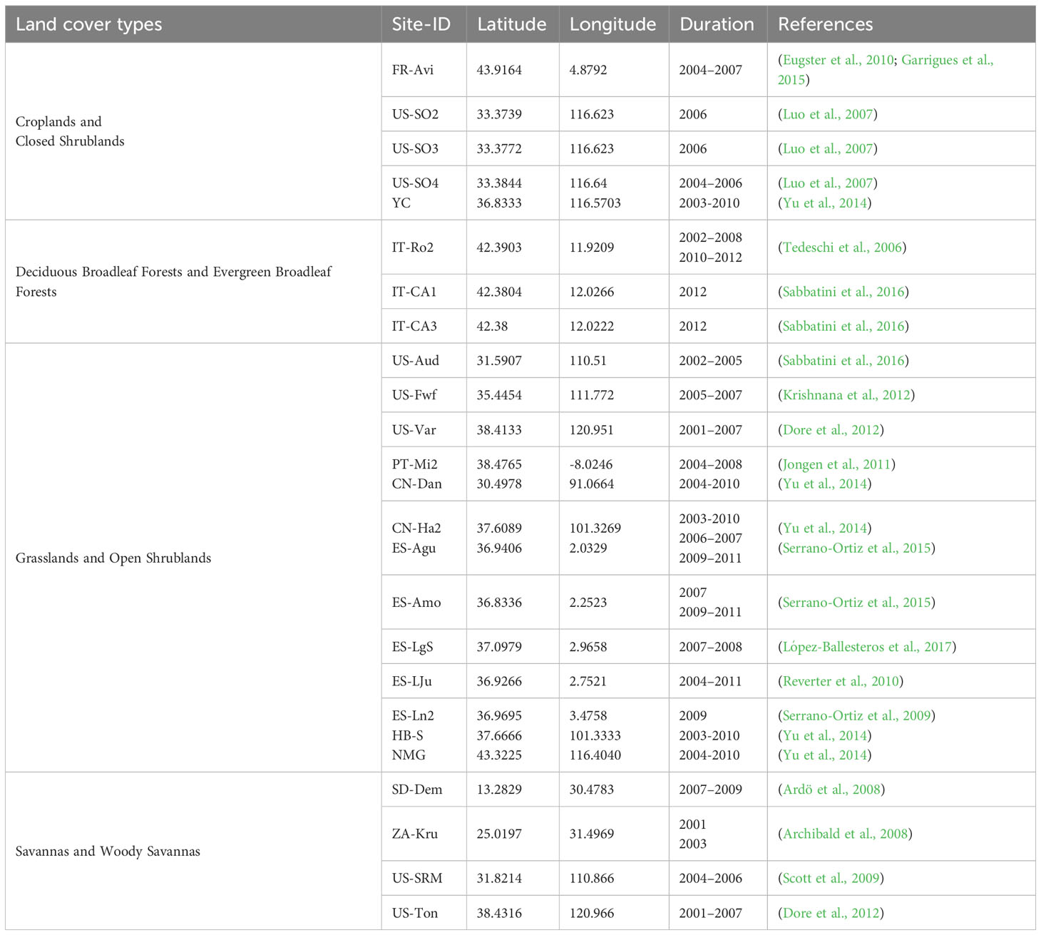
Table 1 Overview of the Fluxnet sites used in this study.

FIGURE 1

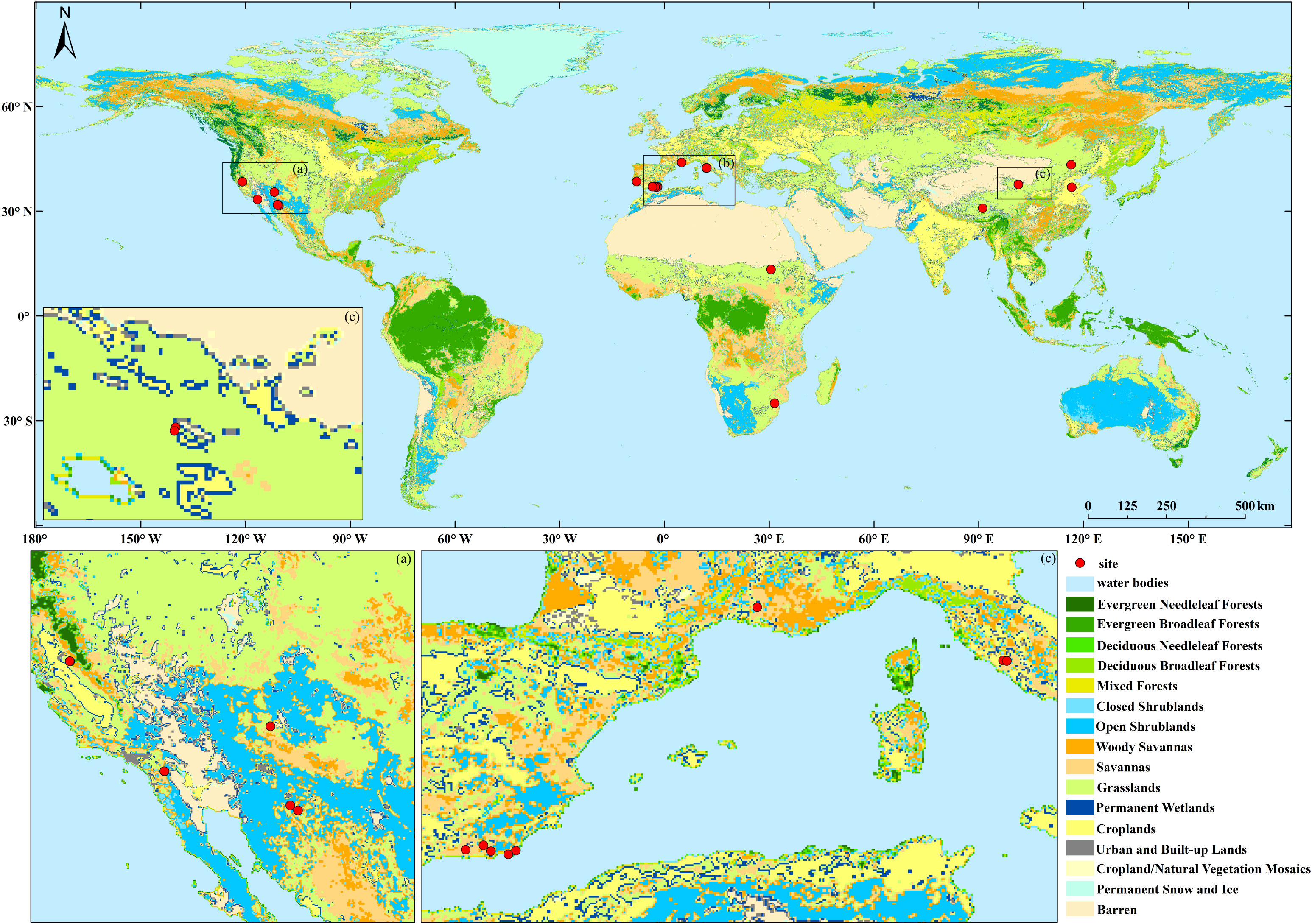
Figure 1 The spatial distribution of flux towers in this study.

MODIS data products, including LE, EVI, and LST, were downloaded from https://modis.ornl.gov/cgi-bin/MODIS/global/subset.pl. We employed the 1km MOD11A2 and MYD11A2 V6.1 LST products, and 500m MOD16A2 and MYD16A2 V6.1 LE products, which are 8-day average values of cloud-free observations featuring day- and night-time estimates, respectively. We omitted observations if the qc flag indicated “bad raw data quality” or if “average LST error > 1 K” (Wan et al., 2021). We conducted quality controls to select valid LE data according to the user guide of MOD16A2.

We used the atmospherically corrected MOD09A1 V6.1 8-day surface reflectance (best observation in 8 days) at 500m resolution to calculate EVI as follows:

$\begin{array}{ll}EVI=\frac{G*({\rho }_{NIR}-{\rho }_{red})}{({\rho }_{NIR}+C_1*{\rho }_{red}-C_2*{\rho }_{blue}+L)}& (3)\end{array}$

where G is a gain factor, ρ is surface reflectance at the Near Infrared (NIR), red and blue band, L is the canopy background adjustment, and C1 and C2 are coefficients of the aerosol resistance term. We adopted coefficient values from the MODIS EVI algorithm, L = 1, C1 = 6, C2 = 7.5, and G = 2.5. EVI over snow is ill-defined; therefore, we masked EVI if the Normalized Difference Snow Index (NDSI) exceeded 0.1 (Salomonson and Appel, 2004). NDSI is calculated as follows:

$\begin{array}{ll}\mathbf{\text{SI}}=\frac{({\rho }_{green}-{\rho }_{SWIR})}{({\rho }_{green}+{\rho }_{SWIR})}& (4)\end{array}$

where ρ is the reflectance in the green and in the Short Wave Infrared band.

Land cover was assessed using the yearly IGBP MCD12Q1 V6.1 500m product. Data were filtered with the quality assessment flag (confidence > 50%) and were averaged across years to one static map.

All 8-day MODIS products were averaged over pixels indicating the same aggregated land cover class within a 3*3km subset. Primarily, we used Terra products, but we also used Aqua data for gap-filling, which we linearly adjusted to account for an offset due to different overpass times. We also compared model simulations with site observations using the MODIS data consistent with the period of the Chinaflux sites DX, HB_S, HB_W, NMG, and YC.

2.2 Method

To account for spatial and seasonal variation separately, we partitioned Reco observations into the site-specific reference respiration rate (Rref) and the remaining standardized respiration rate (Reco_std). Reco_std, or the seasonal variation, was detrended for site-year characteristics, and the seasonal changes were thus smoothed across site-years. Rref is the respiration rate under a reference condition, which describes the basal differences in magnitude among the site-years.

$\begin{array}{ll}Reco=Rref\times Reco\_std& (5)\end{array}$

Reco_std is the ratio of Reco and Rref. Here, firstly, we set the Rref to annual mean Reco (Reco_mean) (formula (6)), and then the Reco_std was calculated by formula (5):

$\begin{array}{ll}Rref=Reco\_mean& (6)\end{array}$

After that we focused on the correlation between Reco_std and the standardized EVI (EVI_std, EVI_std = EVI/EVI_mean), and the correlation between Reco_std and the standardized LE (LE_std, LE_std = LE/LE_mean). In this way, we can remove the site-year differences and understand more accurately the correlation between the seasonal trends of EVI and Reco, as well as the correlation between the seasonal trends of LE and Reco. Through this, we obtained a key indicator (Integrated LE and EVI proxy, hereinafter called ILEP) (formula (7)) to simulate seasonal changes in respiration:

$\begin{array}{ll}ILEP=\frac{P1\times EVI}{EVI\_mean}+\frac{P2\times LE}{LE\_mean}& (7)\end{array}$

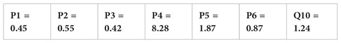
Here P1 and P2 are parameters fixed after cross-validating the model’s robustness and stability.

By relating ILEP to the Q10 model, we obtained the ILEP_Q10 model (formula (8)), and the Rref was then fitted using the ILEP_Q10 model. In the ILEP_Q10 model, the reference variable is set as ILEP, and the reference ILEP point is set to the annual mean value of ILEP (ILEPref = ILEP_mean), thus, Rref is the respiration rate corresponding to the annual mean ILEP.

$\begin{array}{ll}Reco=Rref(ILEPref=ILEP\_mean)*Q{10}^{(\frac{ILEP-ILEP\_mean}{ILEP})}& (8)\end{array}$

In the ILEP_Q10 model, the Q10 value is fixed using the mean value replacement method as done by Ai et al. (2018). Next, we found the correlation between EVI_mean values and the fitted Rref values, as well as the correlation between LE_mean values and the fitted Rref values, and we found that the fitted Rref values were positively, linearly correlated with EVI_mean values and LE_mean values. Based on this, another key indicator – ILEP_RrefP was developed:

$\begin{array}{ll}ILEP\_RrefP=(P3*LE\_mean+P4*EVI\_mean)& (9)\end{array}$

Here P3 is fixed using the fitted Rref values and the corresponding LE_mean values after cross-validation. Likewise, P4 is fixed using the fitted Rref values and the corresponding EVI_mean values after cross-validation.

$\begin{array}{ll}Rref=P5*In(ILEP\_RrefP)+P\mathbf{6}& (10)\end{array}$

After we fixed P3 and P4, the relationship between the calculated ILEP_Rref values and the fitted Rref values was probed, and a logarithmic function (formula (10), hereinafter called ILEP_Rref model) was found to be robust in Rref simulation. P5 and P6 were then fixed after cross-validation.

After all 6 parameters (P1, P2 in formula (7); P3, P4 in formula (9); P5, P6 in formula (10)) are fixed, the final remote sensing Reco model: ILEP_Reco model (formula (11)) was then developed by integrating the ILEP, Q10 model and the ILEP_Rref model:

$\begin{array}{ll}Reco=(P5\times In(P3\times LE\_mean+P4\times EVI\_mean)+P\mathbf{6})\times {(Q\mathbf{10})}^{(\frac{ILEP-ILEP\_mean}{ILEP})}& (11)\end{array}$

2.3 Evaluation of the RS Reco model

All the parameters in these formulas were estimated by non-linearly minimizing the sum of squared residuals, weighted by its uncertainty. The performance of ILEP, ILEP_Rref model, and ILEP_Reco model were explored by cross-validation. The model statistics included the coefficient of determination (R²), root-mean-square error (RMSE), modeling efficiency (EF), and mean bias error (MBE):

$\begin{array}{ll}{R}^2={\left(\frac{{\sum }_{\mathit{\text{i}}=\mathbf{1}}^{\mathit{\text{n}}}(({\mathit{\text{x}}}_{\mathit{\text{i}}}-{\mathit{\text{x}}}^{-})\times ({\mathit{\text{y}}}_{\mathit{\text{i}}}-{\mathit{\text{y}}}^{-}))}{\sqrt{{\sum }_{\mathit{\text{i}}-\mathbf{1}}^{\mathit{\text{n}}}({({\mathit{\text{x}}}_{\mathit{\text{i}}}-{\mathit{\text{x}}}^{-})}^{\mathbf{2}}\times {({\mathit{\text{y}}}_{\mathit{\text{i}}}-{\mathit{\text{y}}}^{-})}^{\mathbf{2}})}}\right)}^2& (12)\end{array}$

$\begin{array}{ll}RMSE=\sqrt{({\sum }_{i=1}^n{(x_i-y_i)}^2)/n}& (13)\end{array}$

$\begin{array}{ll}EF=1-\frac{{\sum }_{\mathbf{\text{i}}=\mathbf{1}}^n{(x_i-y_i)}^{\mathbf{2}}}{{\sum }_{\mathbf{\text{i}}=\mathbf{1}}^n{(x_i-x^{-})}^{\mathbf{2}}}& (14)\end{array}$

$\begin{array}{ll}MBE={\sum }_{\mathbf{\text{i}}=\mathbf{1}}^n(\frac{xi-yi}{n})& (15)\end{array}$

xi is the observed data, yi is the simulated data, and x- and y- are the averages of the observed and simulated data respectively. R stands for the correlation between two variables. R² is the determinant coefficient between two variables. RMSE values were used to measure the biases that caused the simulated data to differ from the observations. EF represents the consistency of the observed values with the simulated ones and is sensitive to the systematic deviation. All fit procedures were done by the least squares method.

A fivefold cross-validation procedure was employed to estimate and validate the parameter set. For each cycle, 80% of the available site-years were used for model calibration and 20% were detained for validation. Each site-year was used for validation exactly once, and the parameters were never evaluated against calibration site-years. Regional-scale ILEP_Reco application was based on parameters retrieved from the entire site data to ensure the most robust parameters.

3 Results

3.1 Exploring and grasping the seasonal changes in Reco

We first explored the relationship between seasonal changes in Reco and EVI and the relationship between seasonal changes in Reco and LE. The results showed that both EVI_std and LE_std were highly correlated with Reco_std (Figure 2). As we can see in Figure 2, the correlation between EVI_std and Reco_std was 0.53, and that between LE_std and Reco_std was 0.55, which indicate that both variables can be used for the simulation of the seasonal variation of Reco.

FIGURE 2

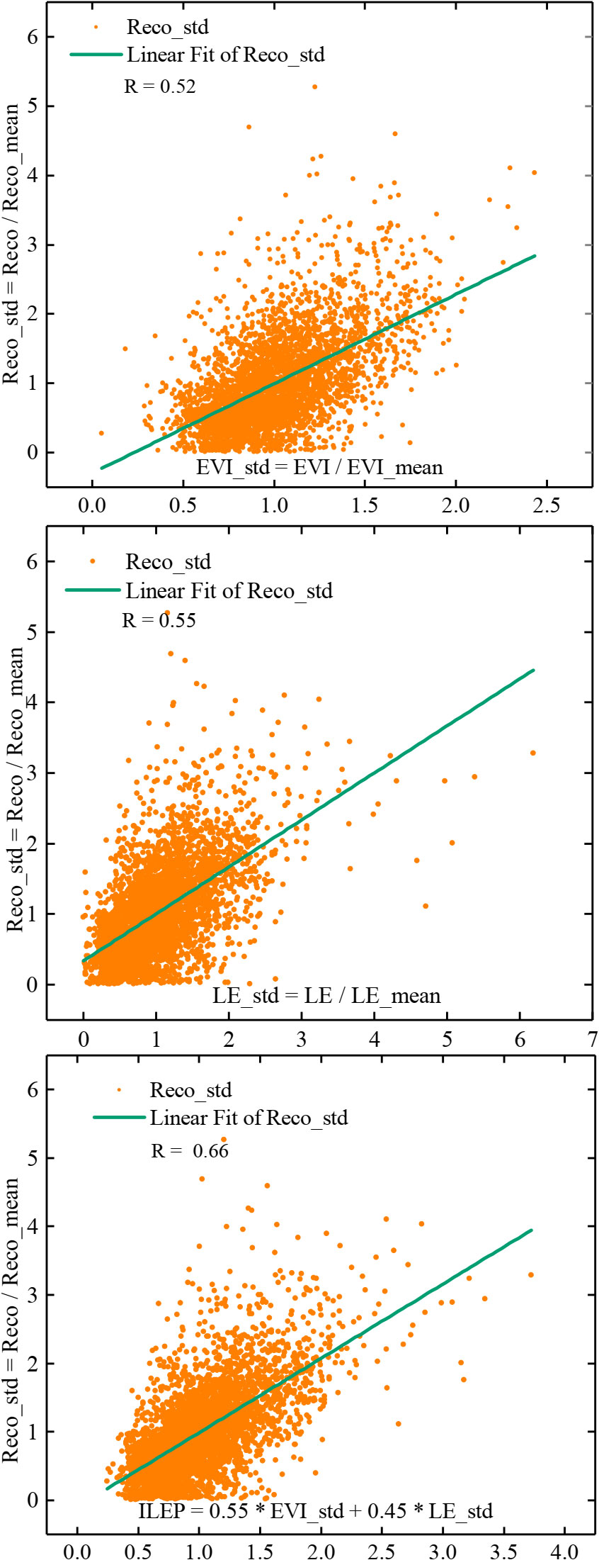
Figure 2 Correlation between Reco_std and EVI_std, between Reco_std and LE_std, and between Reco_std and ILEP (P< 0.01 in all the subplot).

Based on this, the site observations were fitted using the formula (7). It was found that the formula (7) can simulate the seasonal variation of respiration quite well (Table 2). Using 80% of all the site-year data, we fixed P1 and P2 (P1 = 0.55, P2 = 0.45), and thus we obtained ILEP (ILEP = 0.55*EVI/EVI_mean + 0.45*LE/LE_mean). Furthermore, we found that the correlation between ILEP and Reco_std was significantly higher than the correlation between LE_std and Reco_std, or the correlation between EVI_std and Reco_std (Figure 2).

TABLE 2

Table 2 The parameters and performance in the cross-validation of formula (7).

3.2 Fixation of ILEP_Q10 value

Through the conduction above, we obtained a key proxy, ILEP, which was highly correlated with the seasonal variation of Reco. Next, we related ILEP to the Q10 model and obtained the ILEP_Q10 model. We then used the ILEP_Q10 model to fit the observations in each site-year to obtain each site-year’s ILEP_Q10 value. A total of 98 ILEP_Q10 values were finally harvested. The results show that all these 98 ILEP_Q10 values were very conserved.

As is shown in Table 3, the fitted ILEP_Q10 values of each site-year were concentrated near the mean value of 1.24. Therefore, using the mean value replacement method, we fixed the final ILEP_Q10 value in the ILEP_Q10 model to 1.24. Cross-validation revealed the feasibility of using the mean value of the 98 ILEP_Q10 values (1.24) to fix the ILEP_Q10 parameter in the ILEP_Q10 model (Tables 3, 4).

TABLE 3

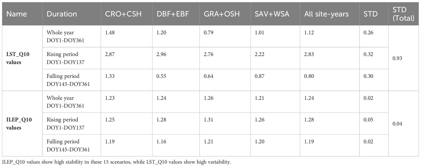
Table 3 The fitted LST_Q10 values and ILEP_Q10 values in 15 scenarios: 3 different time periods (the whole year, the rising period and the falling period) in 5 different site-year types (site-year in 4 ecosystems and all the 98 site-years).

TABLE 4

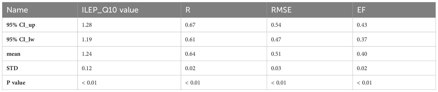
Table 4 The cross-validation results of fixing ILEP_Q10 values using mean value replacement method.

3.3 Construction of ILEP_Rref model

We then obtained the ILEP_Q10 model with a fixed ILEP_Q10 value (i.e., 1.24), and we named it the Q10_fixed_ILEP_Q10 model. By using the Q10_fixed_ILEP_Q10 model, the observations of each site-year were fitted to obtain the Rref (ILEPref = ILEP_mean) value in each site-year. After exploring the relationship between the 98 Rref (ILEPref = ILEP_mean) values and the 98 LE_mean values, as well as the relationship between the 98 Rref (ILEPref = ILEP_mean) and the EVI_mean values, we found that the Rref (ILEPref = ILEP_mean) values were positively and linearly correlated with the LE_mean values and EVI_mean values in the 98 site-years (Figure 3).

FIGURE 3

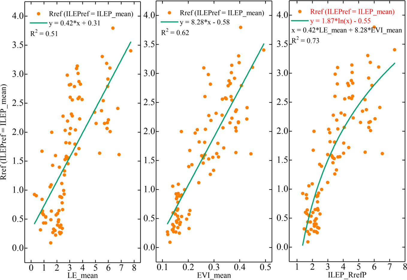
Figure 3 The relationship between the Rref (ILEPref = ILEP_mean) values and EVI_mean values, between the Rref (ILEPref = ILEP_mean) values and LE_mean values, and between the Rref (ILEPref = ILEP_mean) values and ILEP_RrefP (ILEP_RrefP = 0.42*LE_mean + 8.28*EVI_mean) values.

To find suitable ways to simulate the Rref (ILEPref = ILEP_mean) values, we performed the following operations.

1. We used a polynomial surface equation (a*LE_mean + b*EVI_mean + c, a, b, c are the parameters) to fit these Rref (ILEPref = ILEP_mean) values, but against our expectations, the fitted parameter a was below zero, which meant that the LE_mean values were negatively correlated with the Rref (ILEPref = ILEP_mean) values, and that was not consistent with our findings in Figure 3.

2. We then combined the linear equation with fixed parameters to form another key proxy: ILEP_RrefP, i.e., 0.42*LE_mean + 8.28*EVI_mean. The 0.42*LE_mean was derived from the relationship between the Rref (ILEPref = ILEP_mean) values and LE_mean, and the 8.28*EVI_mean was derived from the linear equation between the Rref (ILEPref = ILEP_mean) values and EVI_mean values. Cross-validation showed the feasibility and stability of the ILEP_RrefP (Table 5; Figure 3).

3. After that, we explored the correlation between ILEP_RrefP and the Rref (ILEPref = ILEP_mean) values, and we found a logarithmic model (ILEP_Rref model) between ILEP_RrefP and Rref (ILEPref = ILEP_mean) values. Though it is rather empirical to obtain such an ILEP_Rref model, the relatively narrow changing range in parameters and in correlations of cross-validation showed the feasibility and stability of the ILEP_Rref model (Table 6; Figures 3, 4).

TABLE 5

Table 5 The cross-validation results of the ILEP_RrefP (ILEP_RrefP = P3*LE_mean + P4* EVI_mean).

TABLE 6

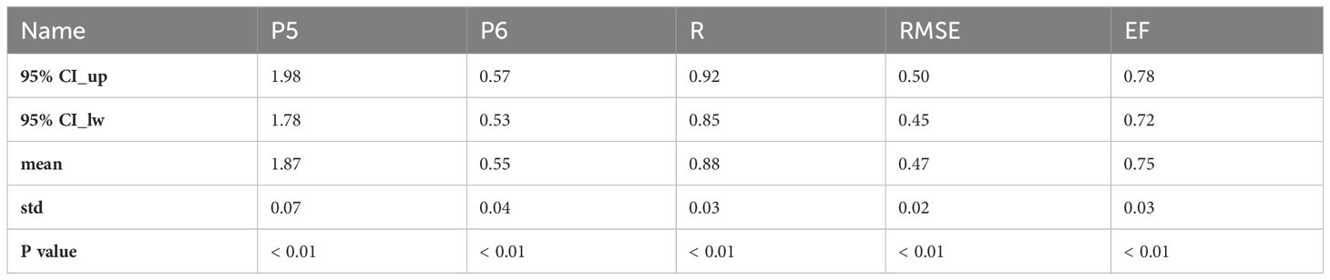
Table 6 The cross-validation results of the ILEP_Rref model (Rref = P5*In(ILEP_RrefP) +P6).

FIGURE 4

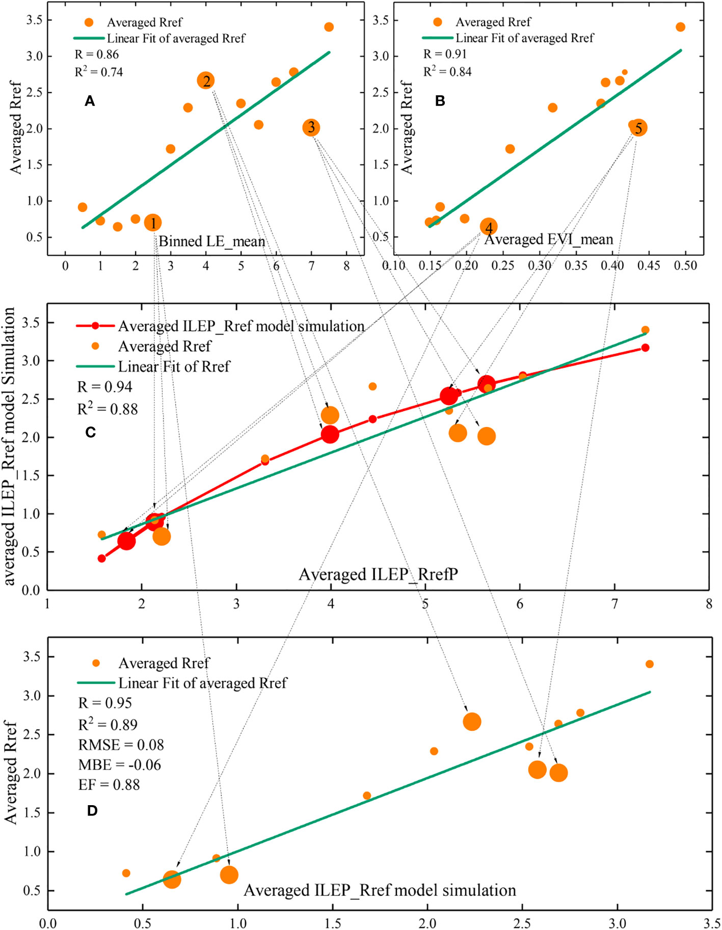
Figure 4 The relationship between the binned LE_mean and the averaged Rref (A), between the binned EVI_mean and the averaged Rref (B), between the averaged ILEP_RrefP and the averaged Rref (C), between the averaged ILEP_Rref model simulation and the averaged Rref (D) (P value < 0.01 in all the subplot). The great complementarity between the EVI_mean and the LE_mean makes ILEP_RrefP show a higher correlation with the averaged Rref.

3.4 Construction of ILEP_Reco model

By using all the site-year observations, the ILEP_Rref model y = P5 * In (ILEP_RrefP) + P6 was fitted to obtain the final parameters P5 and P6 (the cross-validation results are shown in Table 6), and an integration of the ILEP_Rref model, the Q10 model and ILEP finally led to the ILEP_Reco model. Cross-validation showed the feasibility and stability of the ILEP_Reco model, as shown in Table 7.

TABLE 7

Table 7 The cross-validation results of the ILEP_Reco model.

The final ILEP_Reco model and corresponding parameters are described as follows:

$$Reco=(P5\times In(P3\times LE\_mean+P4\times EVI\_mean)+P\mathbf{6})\times {(Q\mathbf{10})}^{(\frac{ILEP-ILEP\_mean}{ILEP})}$$

$$ILEP=\frac{P1\times EVI}{EVI\_mean}+\frac{P2\times LE}{LE\_mean}$$

After comparing the performance of the ILEP_Reco model with that of the Ensemble_all model proposed by Ai et al. (2018), we found that the performance of the ILEP_Reco model (R² = 0.56, RMSE = 1.11 gCm⁻²d⁻¹, EF = 0.46, MBE = −0.06 gCm⁻²d⁻¹) was significantly better than that of the Ensemble_all model (R² = 0.23, RMSE = 1.58 gCm⁻²d⁻¹, EF = −0.08, MBE = −0.11 gCm⁻²d⁻¹) (Figure 5), and the ILEP_Reco model was efficient at grasping the mean state of the seasonal respiration dynamics on a large scale in drylands (R² = 0.91, RMSE = 0.11 gCm⁻²d⁻¹, EF = 0.86, MBE = −0.09 gCm⁻²d⁻¹).

FIGURE 5

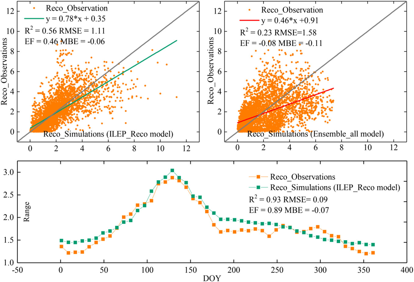
Figure 5 Comparison of the performance of the final ILEP_Reco model with that of the Ensemble_all model in all the 98 site-years’ observations (the upper two subplots show that ILEP_Reco model performs significantly better than the Ensemble_all model, and the lower subplot suggests that ILEP_Reco model is efficient at grasping the mean state of the seasonal respiration dynamics in all the 98 site-years).

4 Discussion

4.1 The seasonal dynamics of Reco and environmental variables

Figure 2 shows that compared with EVI_ std or LE_ std, ILEP (Integrated LE and EVI proxy) can reflect Reco_ std more effectively.

In order to understand this phenomenon more directly, we calculated the Reco_ std, LE_ std, ILEP, and LST_std of all site-years from DOY1 to DOY361 (temporal resolution was 8 days) (Figure 6), and then we calculated the corresponding standard deviation (STD) (error bar in Figure 6).

FIGURE 6

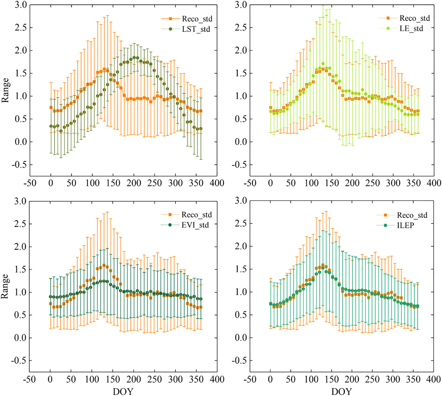
Figure 6 Comparison of seasonal dynamics of Reco_std, LE_std, EVI_std and ILEP. Error bar means standard deviation. Considering the curves and error bars of each variable, ILEP can best reflect the seasonal dynamics of Reco_std, while LST_std shows the largest discrepancy with Reco_std.

A very distinct characteristic in Figure 6 is that EVI_ std, LE_std, and ILEP show a highly similar curve with Reco_std, and they all reach their summits between DOY105 and DOY161, with the maximum values appearing at DOY137. However, the curve of LST_std turns out to be rather different. We found that the curve of LST_std rises more uniformly and reaches its maximum value at DOY 201, and then drops uniformly after DOY 201. In short, in drylands, the curves of Reco_std, LE_std, EVI_std, and ILEP_std all reach their summits in late May, while the curve of LST_std reaches its summit in late July. These indicate that LE_std, EVI_std, and ILEP can well describe the overall seasonal trend of Reco, while LST_std fails to describe it.

The maximum STD values of Reco_std, LE_std, EVI_std, and ILEP in all the site-years all appear around DOY137, and the distribution range of the STD values of ILEP was most similar to that of Reco_std. In contrast, the STD of LST_std was quite different from that of Reco_std. The maximum STD values of LST_std occurred on DOY1, DOY361, and in other low-temperature periods. The above shows that ILEP can better reflect the variation of Reco in each site-year, whereas LST_std can hardly reflect the variation of Reco.

Previous studies have shown that hysteresis between soil CO₂ and soil temperature is controlled by soil water content. In drylands where water supply is not enough, and especially when the temperature is high, strong evapotranspiration may cause a severe water deficit (desiccation), which may lead to the weakening of plant and soil microbial metabolisms and eventually a lower respiration rate (Vargas et al., 2010; Buttlar et al., 2018). Based on this, ILEP shows a high correlation with Reco_std for two reasons.

First, the seasonal trend of EVI actually represents the seasonal change of vegetation canopy (Huete et al., 2002; Costa et al., 2022), so EVI can not only directly characterize the seasonal changes of auto-trophic respiration but also partially characterize the change in hetero-trophic respiration (Goulden et al., 2011; Liu et al., 2022). Hetero-trophic respiration is also highly correlated with vegetation status because vegetation provides a respiratory substrate and a congenial environment for soil microbe metabolism (Kuzyakov, 2002; Grogan and Jonasson, 2005; Thomson et al., 2010; Hopkins et al., 2013; Huo et al., 2017; Azevedo et al., 2021). Previous work has proposed the possibility of using EVI to characterize the seasonal changes of Reco (Rahman et al., 2005), and based on this, models using EVI to characterize seasonal changes of Reco have been developed (Jägermeyr et al., 2014). Therefore, the standardized EVI can well reflect the seasonal trend of respiration.

Second, LE can also reflect Reco’s seasonal changes (Kuppel et al., 2012; de Oliveira et al., 2020). LE refers to the general term for the heat exchange energy between the underlying surface and the atmospheric moisture during the evaporation of soil moisture, the evaporation of water or vegetation, and the transpiration of water in plants (Santanello and Friedl, 2003; Perez-Priego et al., 2017; Chen et al., 2020). In arid regions, especially during the respiration limited period, water is the main limiting factor, and LE can reflect soil moisture and vegetation moisture (Qiu et al., 2016; Williams and Torn, 2016). In addition, LE can also reflect the conductance of the soil–vegetation–atmosphere continuum (SPAC) (Manzoni et al., 2011; Farhadi et al., 2014; Gong et al., 2019). It is indicated that many factors affecting the respiratory process also affect the conductance of SPAC, including land cover types (Costa and Foley, 1997; Jarvis et al., 2013), vegetation richness (Mencuccini et al., 2019), soil porosity (Manzoni et al., 2013) and so forth. Here, we found that the seasonal change in respiration rate was very similar to that in LE (Figure 6), and this result is consistent with the results of previous studies: Reco in arid regions was more strongly correlated with LE than with other temperature-related variables (Ai et al., 2020).

ILEP is the combination of standardized EVI and standardized LE. EVI is a comprehensive reflection of the impact of changes in environmental (temperature, water, light) and biological (phenology, biomass, biological adaptation to the environment) factors on plants. Relatively speaking, EVI can better reflect long-term and stable Reco changes than LE does (Figures 3, 6). LE is a comprehensive reflection of moisture, heat, conductivity of SPAC and so forth. LE can better reflect short-term and flexible Reco changes than EVI does (Figures 2, 6). Together, ILEP can reflect not only long-term and stable Reco changes but also short-term and flexible Reco changes. Therefore, ILEP can well simulate the seasonal changes of Reco (Figures 2, 3, 6).

4.2 Redefinition of Q10 model and Q10 values

We associated ILEP with the Q10 model to obtain the ILEP_Q10 model. In the ILEP_Q10 model, Rref refers to the ecosystem respiration rate corresponding to a reference ILEP value, and the Q10 value is the times of the ecosystem respiration rate change for every 10 units of ILEP change.

By setting the reference ILEP in ILEP_Q10 model as the annual mean ILEP values, we fitted the corresponding ILEP_Q10 values using the observations from 98 site-years. We found that the 98 fitted ILEP_Q10 values showed high stability with a mean value of 1.24 and STD of 0.12, which is consistent with the results of previous works: the fitted LE_Q10 values in 26 cropland sites (a total of 102 site-years) were convergent at 1.20, with a marginal STD of 0.13 (Ai et al., 2020).

To investigate the reasons behind this, we perform the following operations. First, according to the curve of Reco_std in Figure 6, the whole year (DOY1–DOY361) was divided into a Reco_std rising period and a falling period, that is, DOY1–DOY137 was the rising period and DOY145–DOY361 was the falling period. We then used the ILEP_Q10 model to explore the ILEP_Q10 values in 15 scenarios: three different time periods (the whole year, the rising period, and the falling period) in five different site-year types (site-year in four ecosystems and all the 98 site-years).

To further compare the stability of LST_Q10 values and that of ILEP_Q10 values, we associated the LST with the Q10 model to obtain the LST_Q10 model. In the LST_Q10 model, Rref refers to the ecosystem respiration rate corresponding to a reference LST value, and the Q10 value is the times of the ecosystem respiration rate change for every 10 units of LST change. LST_ Ref was selected as the annual mean LST. We used the LST_ Q10 model to explore LST_Q10 values in the same 15 scenarios.

Table 3 shows that the ILEP_Q10 values in 15 scenarios were very stable, with a maximum value of 1.31 and a minimum value of 1.16. The value of all site-years in the whole year was 1.24, and the STD of ILEP_Q10 values from the 15 scenarios was 0.04. In different ecosystems and different time periods, the difference in ILEP_Q10 values was very small, so the mean value of the fitted ILEP_Q10 value of each site-year could be used to replace the ILEP_Q10 value in each site-year. Table 4 also indicates this feasibility.

The LST_Q10 values from the 15 scenarios were very unstable, with a maximum value of 2.96 and a minimum value of 0.55. The value of all site-years in the whole year was 2.83, and the STD of LST_Q10 values from the 15 scenarios was 0.93. LST_Q10 values in the rising period were far greater than those in the falling period. The LST_Q10 values varied greatly in different ecosystems or different time stages. Thus, it is difficult to use the mean value of the fitted LST_Q10 value of each site-year to replace the LST_Q10 value in each site-year.

The redefinition of the Q10 model and the corresponding Q10 value is a novel approach for Reco estimation and facilitates the simulation of Reco on both temporal and spatial scales. The Q10 model is a classic model for biologists to describe the temperature dependence of respiratory rate, and the T_Q10 value is often fixed as a constant 2 when we estimate Reco on a large scale. However, it is suggested that the T_Q10 values vary greatly on both temporal and spatial scales (Davidson and Janssens, 2006; Mahecha et al., 2010; Perkins et al., 2012; Suseela et al., 2012; Meyer et al., 2018; Niu et al., 2021; Kurganova et al., 2022). Spatially, the T_Q10 values tended to be high in the high-latitudinal biomes. The mean T_Q10 values for different biomes ranged from 1.43 to 2.03, with the highest value in tundra and the lowest value in deserts (Zhou et al., 2009), which is consistent with the results of this study. Temporally, the T_Q10 values tended to be higher in the Reco_std rising period and lower in the Reco_std falling period, which coincides with many previous studies (Davidson and Janssens, 2006; Davidson et al., 2006; Suseela et al., 2012; Li et al., 2020; Niu et al., 2021).

The mechanism for this is that the stability of Q10 values is an embodiment of the synchronization of the reference variables with Reco. Reco is actually influenced by many factors, including environmental factors and biological factors (Costa and Foley, 1997; Riveros-Iregui et al., 2007; Jarvis et al., 2013; Manzoni et al., 2013; Mencuccini et al., 2019). Temperature is only one of these environmental factors (Flanagan and Johnson, 2005; Fu et al., 2009; Keenan et al., 2019; Huang et al., 2020), while ILEP is a complex indicator: it changes with the heat, the water, the vegetation, the microbes, the conductance of SPAC, and even the soil properties, which are also the determinants for ecosystem respiratory process (Enquist et al., 2003; Kuzyakov and Larionova, 2005; Davidson et al., 2012; Mamkin et al., 2019; Jia et al., 2020; Li et al., 2020; Hasi et al., 2021; Hu et al., 2021; Jackson et al., 2021; Liu et al., 2021). In other words, ILEP synchronizes with Reco. That is why the ILEP_Q10 exhibited a high degree of stability both on a seasonal scale and a spatial scale. Indeed, the highly conserved ILEP_Q10 values in 98 site-years provided us with a good opportunity for the simulation and estimation of Reco (Ai et al., 2018; Ai et al., 2020).

To sum up, when using the classic Q10 model to simulate Reco, the corresponding T_Q10 values are the apparent temperature sensitivity (the combined effect of a series of factors, such as organism biomass, substrate supply, temperature, and desiccation stress) (Dell et al., 2011; Song et al., 2014), so it is certainly difficult to obtain seasonal and spatial stable Q10 values. Here, we redefined the Q10 model and Q10 values and proposed the ILEP_Q10 model and corresponding ILEP_Q10 values based on the core variable – ILEP, which effectively reduced the spatial and temporal heterogeneity of the Q10 values.

4.3 Reco’s spatial change and simulation

The spatial variation of Reco reflects differences in site conditions, including organisms and the environment. Both long-term (hundreds to thousands of years) climate regime and short-term (a few days to months) climate extremes have impacts on Reco’s spatial variation (Monson et al., 2006; Hoover et al., 2016). In the process of Reco simulation, Rref is often used to characterize the spatial variability of Reco (Reichstein et al., 2003; Chen et al., 2010; Ai et al., 2018; Ai et al., 2020).

To calculate the Rref, the first problem is to determine the reference variable. The reference variable must have an important relationship with the seasonal variation of Reco. The reference variables in the previous Reco models are temperature or LST. When Rref is set to the Reco that corresponds to the annual average temperature, Rref (Tref = T_mean) is found to be highly correlated with simple vegetation index and temperature (Ai et al., 2018), as temperature is the most fundamental climatic factor influencing the kinetics of biochemical reactions. Thus, when the reference temperature is fixed at the mean annual value, Rref will reflect an average state of physiological processes both in plants and in microbes (Bond-Lamberty and Thomson, 2010; Mahecha et al., 2010; Buckley and Huey, 2016; Jian et al., 2020; Johnston et al., 2021; Stell et al., 2021).

However, the findings and explanations above do not work in drylands. Ai et al. (2020) argue that temperature is not necessarily the only reference variable: there can be other variables that are more correlated with Reco in drylands. Furthermore, in this study, if the reference variable was set as the ILEP, and the reference point was set to the annual mean ILEP, then the ILEP_Rref was actually the Reco that corresponded to the annual mean ILEP.

Based on this, Rref (ILEPref=ILEP_mean) was found to be highly correlated with the annual mean LE and the annual mean EVI (Figure 3). The EVI_mean reflects the average annual vegetation condition, which affects not only vegetation respiration but also microbial respiration (Huete et al., 2002; Goulden et al., 2011; Costa et al., 2022; Liu et al., 2022). The LE_mean reflects not only the average heat and water condition (the main limiting factor of respiration in the arid area), but also the average conductance state of SPAC (Santanello and Friedl, 2003; Manzoni et al., 2011; Farhadi et al., 2014; Perez-Priego et al., 2017; Chen et al., 2020). Therefore, both the EVI_mean and LE_mean are highly correlated with Rref (ILEPref=ILEP_mean).

In order to further explore 1) the relationship between the Rref (ILEPref=ILEP_mean) values and annual mean LE values, 2) the relationship between the Rref (ILEPref=ILEP_mean) values and annual mean EVI values, 3) the relationship between the Rref (ILEPref=ILEP_mean) values and ILEP_RrefP (ILEP_RrefP=0.42*LE_mean+8.38*EVI_mean) values, and 4) the relationship between the Rref (ILEPref=ILEP_mean) values and the simulations of ILEP_Rref model, we

1) calculated the annual mean LE values (LE_mean), the annual mean EVI values (EVI_mean), the annual ILEP_ RrefP values, and the simulations of ILEP_Rref model (see below) in all the 98 site-years:

$$Rref=1.87\times In(0.42\times LE\_mean+8.28\times EVI\_mean)+0.87$$

2) fitted the Rref (ILEPref=ILEP_mean) values of each site-year using the following equations, and a total of 98 Rref (ILEPref=ILEP_mean) values were obtained:

$$Reco=Rref\times {(Q10)}^{(\frac{ILEP-ILEP\_mean}{ILEP})}$$

$$ILEP=\frac{0.45\times EVI}{EVI\_mean}+\frac{0.55\times LE}{LE\_mean}$$

and 3) explored the correlation between annual mean LE (LE_mean) and the averaged Rref (ILEPref=ILEP_mean) values using the bin-average method. The LE_mean values in all the 98 site-years were binned at 0.5 intervals, and the corresponding Rref (ILEPref=ILEP_mean) values at each 0.03 interval were averaged. After that, we obtained 14 pairs of binned LE_mean values and the corresponding averaged Rref (ILEPref=ILEP_mean) values, and found the correlation between them. Likewise, we found the correlation between EVI_mean values and the averaged Rref (ILEPref=ILEP_mean) values, the correlation between ILEP_RrefP (0.42*LE_mean + 8.28*EVI_mean) values and the averaged Rref (ILEPref=ILEP_mean) values, and the correlation between the simulations of the ILEP_Rref model and the averaged Rref (ILEPref=ILEP_mean) values.

Figure 4 shows that 1) the correlation between EVI_mean and bin-averaged Rref was higher than that between LE_mean and bin-averaged Rref; 2) the correlation between ILEP_RrefP and bin-averaged Rref was higher than that between EVI_mean and bin-averaged Rref; and 3) the correlation between ILEP_RrefP and bin-averaged Rref was higher than that between the LE_mean and bin-averaged Rref.

In order to further explore the reasons behind the findings above, we selected three outliers in subplot (a) and two outliers in subplot (b) that deviated sharply from the fitting lines, and explored the situation of these five outliers in subplot (c) and subplot (d).

The results showed that, except for outlier 3 in subplot (c) and subplot (d), which still deviated from the fitting line severely, the other four outliers in subplot (c) and subplot (d) no longer deviated from the fitting line sharply; instead, these four outliers were even quite close to the fitting line (such as outlier 1). This indicates that the deviation degree of these outliers was reduced. Specifically, the deviation of outlier 1 and outlier 2 was weakened by EVI_ mean in subplot (c) and subplot (d), and the deviation of outlier 4 and outlier 5 was weakened by LE_mean in subplot (c) and subplot (d). In other words, it was the great complementarity between EVI_mean and LE_mean that makes ILEP_RrefP show a higher correlation with the Rref (ILEPref=ILEP_mean) values.

We mapped our model to the scale of northern China drylands. We further compared the ILEP_Reco simulations with the in situ Reco observations in Chinaflux sites DX, HB_S, HB_W, NMG and YC. The results showed that the ILEP_Reco model can robustly picture the spatial-temporal distribution of Reco there (Figures 7, 8), where R² = 0.62, and RMSE = 1.20 gCm⁻²d⁻¹. There were differences in the spatial distribution of Reco there, ranging from 0.003 to 4.230 gCm⁻²d⁻¹, roughly showing an increasing trend from northwest to southeast. The minimum value appeared in the Junggar Basin of Xinjiang, and the maximum value appeared in the middle of the semi-arid region (the border area between Qinghai and Gansu) (Figure 7). The main reason was that the vegetation in the southeast is relatively lush, while the vegetation coverage in the northwest is low. The spatial distribution of the monthly average ILEP_ Reco from 2003 to 2010 and annual average ILEP_Reco were similar, but there were seasonal differences. In central Inner Mongolia, the edge of the Junggar Basin, central Tibet, and Loess Plateau, seasonal differences are small. These areas are mainly grasslands and sparsely vegetated areas. The low vegetation coverage there leads to small seasonal differences in Reco. However, in the eastern part of the Altai Mountains, Mount Tianshan, Himalayas, and semi-arid areas, the seasonal differences are large, since these areas are mainly mixed zones of forests and agricultural grasslands. The respiration of forests is strong, and environmental factors such as temperature and precipitation can affect vegetation respiration. Besides, farmland, influenced by human management, also exhibits significant seasonal differences. The maximum Reco values on a monthly scale mainly occur between July and August. Specifically, 82.75% of the research area reaches the highest values between July and August (Figure 8). During this period, vegetation growth is vigorous, and water and heat conditions are relatively good, resulting in higher Reco. Furthermore, 71.85% of the area has the smallest values between January and April (Figure 8). During this period, vegetation is in a slow growth period and is also affected by low precipitation or temperature, resulting in lower Reco.

FIGURE 7

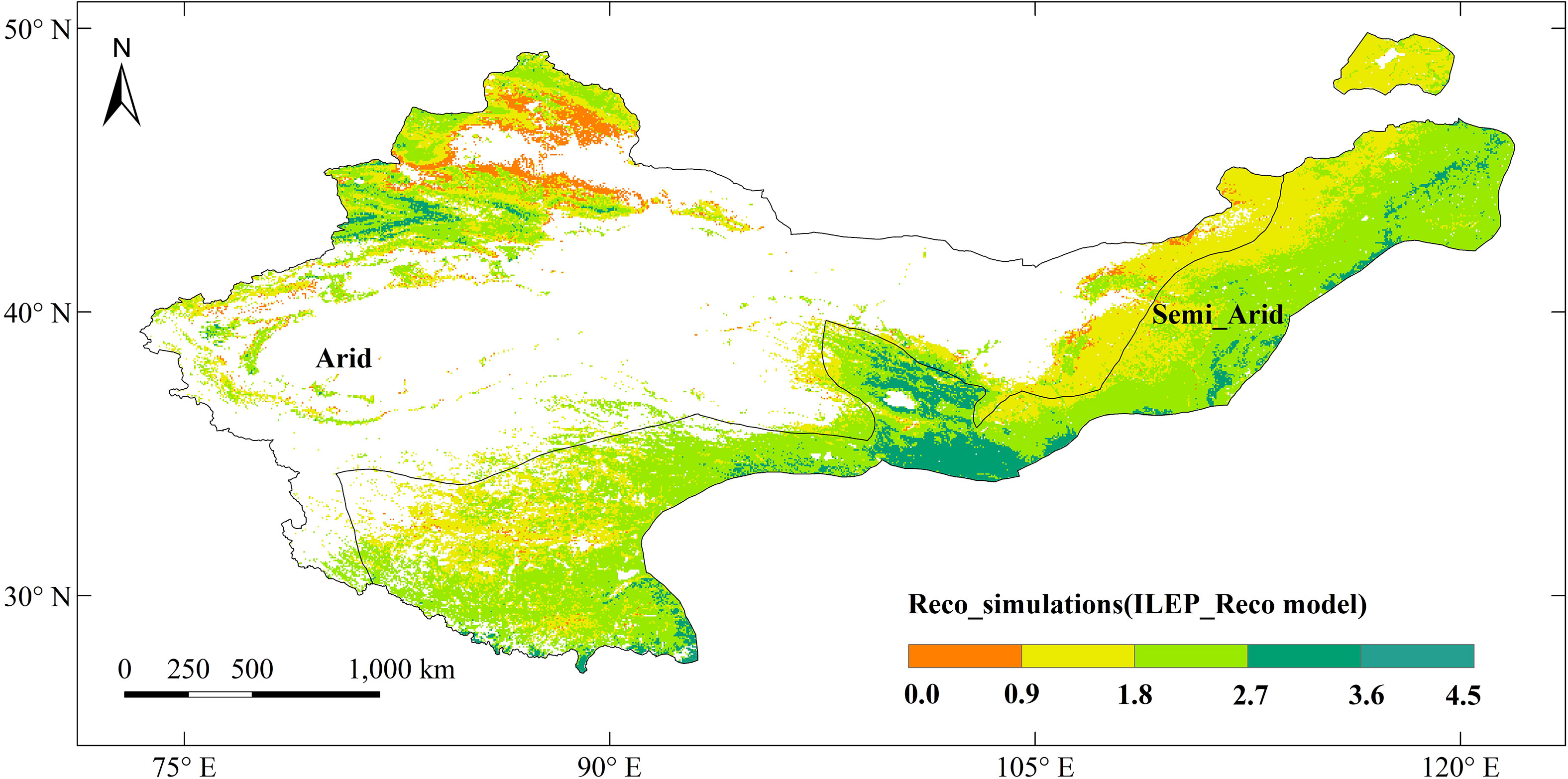
Figure 7 The annual spatial distribution of Reco simulated by the ILEP_Reco model (gCm⁻²d⁻¹).

FIGURE 8

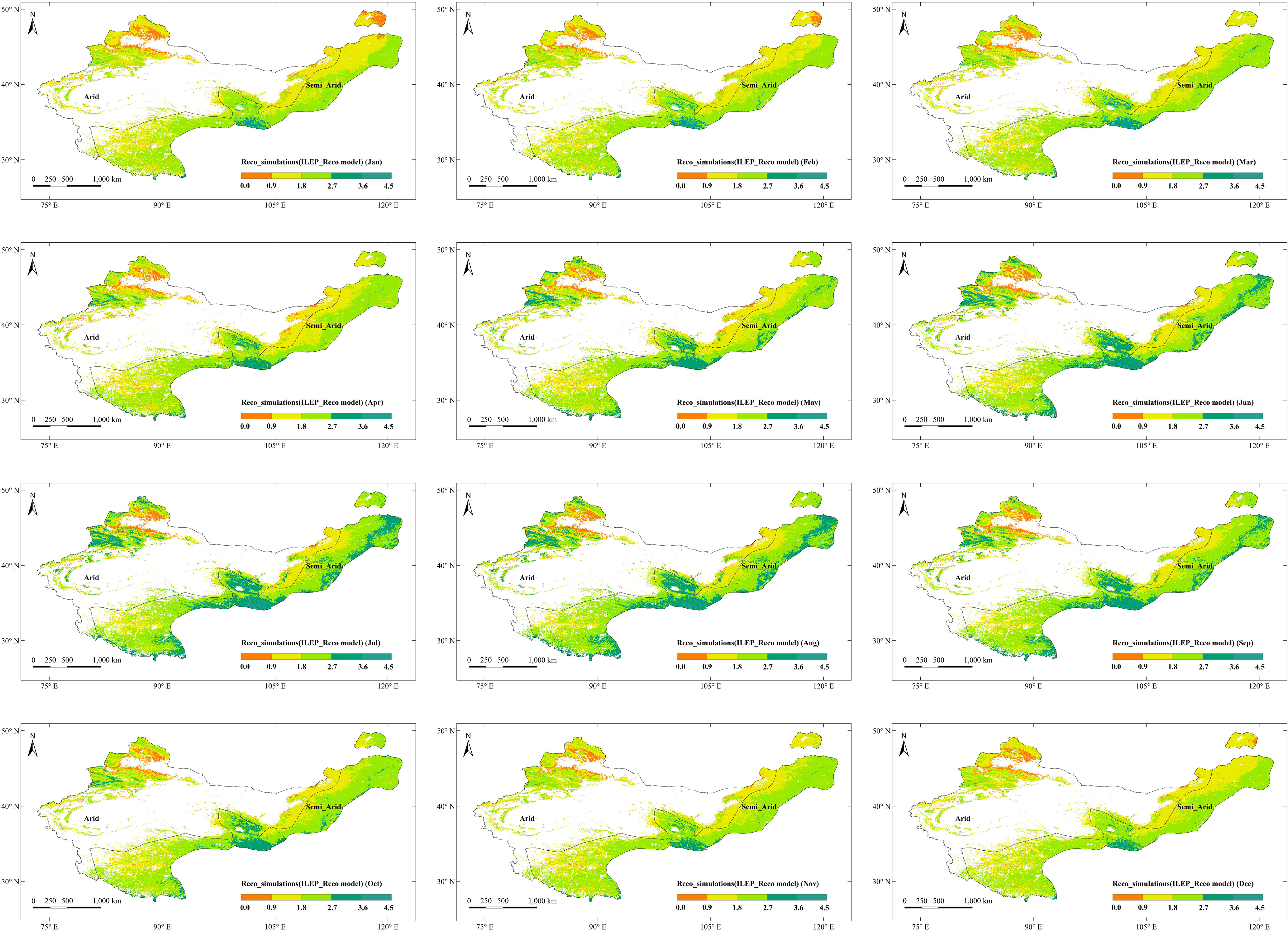
Figure 8 The monthly spatial distribution of Reco simulated by the ILEP_Reco model (gCm⁻²d⁻¹).

4.4 Uncertainty

Although a purely remote Reco model – ILEP_Reco – is proposed in this study, we still argue there is uncertainty in respiration simulation in drylands. There are several reasons for this. 1) The number of flux observations in drylands is relatively small. In the global flux system, most flux sites are concentrated in the middle and high latitude non-arid areas, but the arid regions exceed 40% of the land, which further reduces the flux density in dry areas. 2) There is also uncertainty in MODIS products themselves. Especially for the large-scale inversion of LE data, there is still relatively large uncertainty at present. 3) The flux respiration data are still not true observations, but a kind of interpolation or extrapolation from an exponential relationship between nighttime flux data and temperature. Because the correlation between nighttime flux data and temperature in arid regions is very weak, errors will occur in respiration interpolation or extrapolation.

5 Conclusions

This study demonstrates that: 1) In drylands, standardized EVI and LE show a high correlation with the seasonal dynamic pattern of ecosystem respiration, and a key indicator ILEP can well simulate the seasonal change of the Reco there. 2) When we relate ILEP with the classic Q10 model, the ILEP_Q10 values are highly concentrated, which greatly facilitates us to replace the ILEP_Q10 parameter of each site-year with a fixed ILEP_Q10 value. 3) After we replace the ILEP_Q10 value of each site-year with a fixed value, the Rref values fitted by each site-year’s in situ observations, i.e., the Reco corresponding to the annual mean ILEP, are highly correlated with the annual mean EVI and annual mean LE. Based on another key indicator ILEP_RrefP, a simple remote sensing Rref model (ILEP_Rref model) was developed, which can efficiently simulate the site-year specific Rref values. 4) Based on the above, a MODIS remote sensing model (ILEP_Reco model) with only 6 parameters was developed, which can simulate the spatio-temporal dynamics of Reco in drylands powerfully, with R² = 0.56, RMSE = 1.12 gCm⁻²d⁻¹, EF = 0.46, MBE = −0.06 gCm⁻²d⁻¹, and performs much better than the previous models, such as Ensemble_all. 5) This ILEP_Reco model vividly depicts the spatial-temporal distribution of Reco in northern China drylands with an 8-day 1km resolution. Therefore, this study goes a step further in the field of the remote sensing estimation of ecosystem respiration in arid areas.

Data availability statement

Publicly available datasets were analyzed in this study. This data can be found here: http://www.fluxdata.org/ and https://modis.ornl.gov/cgi-bin/MODIS/global/subset.pl.

Author contributions

Conceptualization, JA, XQ, and JZ; methodology, MH and RZ; software, RZ, XQ, and JL; validation, HW, RX, and SS; formal analysis, JL and HW; investigation, HW and YL; resources, JA and HW; data curation, XQ, JA, and HW; writing—original draft preparation, JA; writing—review and editing, HW, JL, and RX; visualization, RX and MH; supervision, HW,JA, and YL; project administration, HW and RX; funding acquisition, JZ and JA. All authors contributed to the article and approved the submitted version.

Funding

This research was jointly supported by the Hainan Provincial Natural Science Foundation of China (Grant No. 422CXTD532), the Hunan Youth Talent Promotion Program (Grant No. 2023TJ-N05), the Yiyang Youth Talent Promotion Program (YYTPP202205) and the Key R&D Projects of the ShuGuang Plan (YYZYSZ2023004).

Conflict of interest

The authors declare that the research was conducted in the absence of any commercial or financial relationships that could be construed as a potential conflict of interest.

Publisher’s note

All claims expressed in this article are solely those of the authors and do not necessarily represent those of their affiliated organizations, or those of the publisher, the editors and the reviewers. Any product that may be evaluated in this article, or claim that may be made by its manufacturer, is not guaranteed or endorsed by the publisher.

References

Ai J., Jia G., Epstein H. E., Wang H., Zhang A., Hu Y. (2018). MODIS-based estimates of global terrestrial ecosystem respiration. J. Geophys. Res. Biogeosci. 123 (2), 326–352. doi: 10.1002/2017JG004107

CrossRef Full Text | Google Scholar

Ai J., Xiao S., Feng H., Wang H., Hu Y. (2020). A global terrestrial ecosystem respiration dataset, (2001-2010) estimated with MODIS land surface temperature and vegetation indices. Big Earth Data. 4 (2), 142–152. doi: 10.1080/20964471.2020.1768001

CrossRef Full Text | Google Scholar

Archibald S., Kirton A., van der Merwe M., Scholes R. J., Williams C. A., Hanan N. (2008). Drivers of interannual variability in Net Ecosystem Exchange in a semi-arid savanna ecosystem, South Africa. Biogeosci. Discuss. 54 (4), 3221–3266. doi: 10.5194/bgd-5-3221-2008

CrossRef Full Text | Google Scholar

Ardö J., Mölder M., El-Tahir B. A., Elkhidir H. A. (2008). Seasonal variation of carbon fluxes in a sparse savanna in semi-arid Sudan. Carbon Balanc. Manage. 3, 7. doi: 10.1186/1750-0680-3-7

CrossRef Full Text | Google Scholar

Azevedo O., Parker T. C., Siewert M. B., Subke J. A. (2021). Predicting soil respiration from plant productivity (NDVI) in a sub-arctic tundra ecosystem. Remote Sens. 13 (13), 2571. doi: 10.3390/rs13132571

CrossRef Full Text | Google Scholar

Bahn M., Reichstein M., Davidson E. A., Grünzweig J., Jung M., Carbone M. S., et al. (2010). Soil respiration at mean annual temperature predicts annual total across vegetation types and biomes. Biogeosciences 7 (7), 2147–2157. doi: 10.5194/bg-7-2147-2010

PubMed Abstract | CrossRef Full Text | Google Scholar

Baldocchi D. (2003). Assessing the eddy covariance technique for evaluating carbon dioxide exchange rates of ecosystems: past, present and future. Glob. Change Biol. 9 (4), 479–492. doi: 10.1002/(SICI)1096-8652(199710)56:23.0.CO;2-Y

CrossRef Full Text | Google Scholar

Baldocchi D. (2008). Breathing of the terrestrial biosphere: lessons learned from a global network of carbon dioxide flux measurement systems. Aust. J. Bot. 56 (1), 1–26. doi: 10.1071/BT07151

CrossRef Full Text | Google Scholar

Bond-Lamberty B., Thomson A. (2010). Temperature-associated increases in the global soil respiration record. Nature 464 (7288), 579–582. doi: 10.1038/nature08930

PubMed Abstract | CrossRef Full Text | Google Scholar

Buckley L. B., Huey R. B. (2016). Temperature extremes: geographic patterns, recent changes, and implications for organismal vulnerabilities. Glob. Change Biol. 22 (12), 3829–3842. doi: 10.1111/gcb.13313

CrossRef Full Text | Google Scholar

Buttlar J. V., Zscheichler J., Rammig A., Sippel S., Mahecha M. D. (2018). Impacts of droughts and extreme-temperature events on gross primary production and ecosystem respiration: a systematic assessment across ecosystems and climate zones. Biogeosci. Discuss. 15 (5), 1–39. doi: 10.5194/bg-15-1293-2018

CrossRef Full Text | Google Scholar

Chen Q., Wang Q., Han X., Wan S., Li L. (2010). Temporal and spatial variability and controls of soil respiration in a temperate steppe in northern China. Glob. Biogeochem. Cycle 24 (2), GB2010. doi: 10.1029/2009GB003538

CrossRef Full Text | Google Scholar

Chen J., Wen J., Kang S., Meng X., Yuan Y. (2020). Assessments of the factors controlling latent heat flux and the coupling degree between an alpine wetland and the atmosphere on the Qinghai-Tibetan Plateau in summer. Atmos. Res. 240 (6–7), 104937. doi: 10.1016/j.atmosres.2020.104937

CrossRef Full Text | Google Scholar

Costa M. H., Foley J. A. (1997). Water balance of the Amazon Basin: Dependence on vegetation cover and canopy conductance. J. Geophys. Res. Atmos. 102 (D20), 23973–23989. doi: 10.1029/97JD01865

CrossRef Full Text | Google Scholar

Costa G. B., Mendes K. R., Viana L. B., Almeida G. V., Mutti P. R., E Silva C. M. S., et al. (2022). Seasonal ecosystem productivity in a seasonally dry tropical forest (Caatinga) using flux tower measurements and remote sensing data. Remote Sens. 14 (16), 3955. doi: 10.3390/rs14163955

CrossRef Full Text | Google Scholar

Dacal M., Bradford M. A., Plaza C., Maestre F. T., García-Palacios P. (2019). Soil microbial respiration adapts to ambient temperature in global drylands. Nat. Ecol. Evol. 3 (2), 232–238. doi: 10.1038/s41559-018-0770-5

PubMed Abstract | CrossRef Full Text | Google Scholar

Davidson E. A., Janssens I. A. (2006). Temperature sensitivity of soil carbon decomposition and feedbacks to climate change. Nature 440 (7081), 165–173. doi: 10.1038/nature04514

PubMed Abstract | CrossRef Full Text | Google Scholar

Davidson E. A., Janssens I. A., Luo Y. (2006). On the variability of respiration in terrestrial ecosystems: moving beyond Q10. Glob. Change Biol. 12 (2), 154–164. doi: 10.1111/j.1365-2486.2005.01065.x

CrossRef Full Text | Google Scholar

Davidson E. A., Samanta S., Caramori S. S., Savage K. (2012). The Dual Arrhenius and Michaelis–Menten kinetics model for decomposition of soil organic matter at hourly to seasonal time scales. Glob. Change Biol. 18 (1), 371–384. doi: 10.1111/j.1365-2486.2011.02546.x

CrossRef Full Text | Google Scholar

Dell A. I., Pawar S., Savage V. M. (2011). Systematic variation in the temperature dependence of physiological and ecological traits. Proc. Natl. Acad. Sci. U. S. A. 108 (26), 10591–10596. doi: 10.1073/pnas.1015178108

PubMed Abstract | CrossRef Full Text | Google Scholar

de Oliveira G., Brunsell N. A., Crews T. E., DeHaan L. R., Vico G. (2020). Carbon and water relations in perennial Kernza (Thinopyrum intermedium): An overview. Plant Sci. 295, 110279. doi: 10.1016/j.plantsci.2019.110279

PubMed Abstract | CrossRef Full Text | Google Scholar

Dore S., Montes-Helu M., Hart S. C., Hungate B. A., Koch G. W., Moon J. B., et al. (2012). Recovery of ponderosa pine ecosystem carbon and water fluxes from thinning and stand-replacing fire. Glob. Change Biol. 18 (10), 3171–3185. doi: 10.1111/j.1365-2486.2012.02775.x

CrossRef Full Text | Google Scholar

Enquist B. J., Economo E. P., Huxman T. E., Allen A. P., Ignace D. D., Gillooly J. F. (2003). Scaling metabolism from organisms to ecosystems. Nature 423 (6940), 639–642. doi: 10.1038/nature01671

PubMed Abstract | CrossRef Full Text | Google Scholar

Eugster W., Moffat A. M., Ceschia E., Aubinet M., Ammann C., Osborne B., et al. (2010). Management effects on European cropland respiration. Agric. Ecosyst. Environ. 139 (3), 346–362. doi: 10.1016/j.agee.2010.09.001

CrossRef Full Text | Google Scholar

Farhadi L., Entekhabi D., Salvucci G., Sun J. (2014). Estimation of land surface water and energy balance parameters using conditional sampling of surface states. Water Resour. Res. 50 (2), 1805–1822. doi: 10.1002/2013WR014049

CrossRef Full Text | Google Scholar

Flanagan L. B., Johnson B. G. (2005). Interacting effects of temperature, soil moisture and plant biomass production on ecosystem respiration in a northern temperate grassland. Agric. For. Meteorol. 130 (3), 237–253. doi: 10.1016/j.agrformet.2005.04.002

CrossRef Full Text | Google Scholar

Fu Y., Zheng Z., Yu G., Hu Z., Sun X., Shi P., et al. (2009). Environmental influences on carbon dioxide fluxes over three grassland ecosystems in China. Biogeosciences 6 (12), 2879–2893. doi: 10.5194/bg-6-2879-2009

CrossRef Full Text | Google Scholar

Garrigues S., Olioso A., Calvet J. C., Martin E., Renard D. (2015). Evaluation of land surface model simulations of evapotranspiration over a 12 year crop succession: impact of the soil hydraulic properties. Hydrol. Earth Syst. Sci. 19 (7), 3109–3131. doi: 10.5194/hessd-11-11687-2014

CrossRef Full Text | Google Scholar

Gillooly J. F., Brown J. H., West G. B., Savage V. M., Charnov E. L. (2001). Effects of size and temperature on metabolic rate. Science 293 (5538), 2248–2251. doi: 10.1126/science.1061967

PubMed Abstract | CrossRef Full Text | Google Scholar

Gong C., Song C., Zhang D., Zhang J. (2019). Litter manipulation strongly affects CO2 emissions and temperature sensitivity in a temperate freshwater marsh of northeastern China. Ecol. Indic. 97, 410–418. doi: 10.1016/j.ecolind.2018.10.021

CrossRef Full Text | Google Scholar

Goulden M. L., Mcmillan A. M. S., Winston G. C., Rocha A. V., Manies K. L., Harden J. W., et al. (2011). Patterns of NPP, GPP, respiration, and NEP during boreal forest succession. Glob. Change Biol. 17 (2), 855–871. doi: 10.1111/j.1365-2486.2010.02274.x

CrossRef Full Text | Google Scholar

Grogan P., Jonasson S. (2005). Temperature and substrate controls on intra-annual variation in ecosystem respiration in two subarctic vegetation types. Glob. Change Biol. 11 (3), 465–475. doi: 10.1111/j.1365-2486.2005.00912.x

CrossRef Full Text | Google Scholar

Grünzweig J. M., De Boeck H. J., Rey A., Santos M. J., Adam O., Bahn M., et al. (2022). Dryland mechanisms could widely control ecosystem functioning in a drier and warmer world. Nat. Ecol. Evol. 6 (8), 1064–1076. doi: 10.1038/s41559-022-01779-y

PubMed Abstract | CrossRef Full Text | Google Scholar

Hasi M., Zhang X., Niu G., Wang Y., Geng Q., Quan Q., et al. (2021). Soil moisture, temperature and nitrogen availability interactively regulate carbon exchange in a meadow steppe ecosystem. Agric. For. Meteorol. 304-305, 108389. doi: 10.1016/j.agrformet.2021.108389

CrossRef Full Text | Google Scholar

Heimann M., Reichstein M. (2008). Terrestrial ecosystem carbon dynamics and climate feedbacks. Nature 451 (7176), 289–292. doi: 10.1038/nature06591

PubMed Abstract | CrossRef Full Text | Google Scholar

Heskel M. A., O’Sullivan O. S., Reich P. B., Tjoelker M. G., Weerasinghe L. K., Penillard A., et al. (2016). Convergence in the temperature response of leaf respiration across biomes and plant functional types. Proc. Natl. Acad. Sci. U. S. A. 113 (14), 3832–3837. doi: 10.1073/pnas.1520282113

PubMed Abstract | CrossRef Full Text | Google Scholar

Hoover D. L., Knapp A. K., Smith M. D. (2016). The immediate and prolonged effects of climate extremes on soil respiration in a mesic grassland. J. Geophys. Res. Biogeosci. 121 (4), 1034–1044. doi: 10.1002/2015JG003256

CrossRef Full Text | Google Scholar

Hopkins F., Gonzalez-Meler M. A., Flower C. E., Lynch D. J., Czimczik C., Tang J., et al. (2013). Ecosystem-level controls on root-rhizosphere respiration. New Phytol. 199 (2), 339–351. doi: 10.1111/nph.12271

PubMed Abstract | CrossRef Full Text | Google Scholar

Hu Z., Zhang J., Du Y., Shi K., Ren G., Iqbal B., et al. (2021). Substrate availability regulates the suppressive effects of Canada goldenrod invasion on soil respiration. J. Plant Ecol. 15 (3), 509–523. doi: 10.1093/jpe/rtab073

CrossRef Full Text | Google Scholar

Huang N., Wang L., Song X., Black T. A., Jassal R. S., Myneni R. B., et al. (2020). Spatial and temporal variations in global soil respiration and their relationships with climate and land cover. Sci. Adv. 6 (41), eabb8508. doi: 10.1126/sciadv.abb8508

PubMed Abstract | CrossRef Full Text | Google Scholar

Huete A., Didan K., Miura T., Rodriguez E. P., Gao X., Ferreira L. G. (2002). Overview of the radiometric and biophysical performance of the MODIS vegetation indices. Remote Sens. Environ. 83 (1-2), 195–213. doi: 10.1016/S0034-4257(02)00096-2

CrossRef Full Text | Google Scholar

Huo C., Luo Y., Cheng W. (2017). Rhizosphere priming effect: A meta-analysis. Soil Biol. Biochem. 111, 78–84. doi: 10.1016/j.soilbio.2017.04.003

CrossRef Full Text | Google Scholar

Ikawa H., Nakai T., Busey R. C., Kim Y., Kobayashi H., Nagai S., et al. (2015). Understory CO2, sensible heat, and latent heat fluxes in a black spruce forest in interior Alaska. Agric. For. Meteorol. 214, 80–90. doi: 10.1016/j.agrformet.2015.08.247

CrossRef Full Text | Google Scholar

Irvine J., Law B. E., Kurpius M. R. (2005). Coupling of canopy gas exchange with root and rhizosphere respiration in a semi-arid forest. Biogeochemistry 73, 271–282. doi: 10.1007/s10533-004-2564-x

CrossRef Full Text | Google Scholar

Jackson M. C., Pawar S., Woodward G. (2021). The temporal dynamics of multiple stressor effects: from individuals to ecosystems. Trends Ecol. Evol. 36 (5), 402–410. doi: 10.1016/j.tree.2021.01.005

PubMed Abstract | CrossRef Full Text | Google Scholar

Jägermeyr J., Gerten D., Lucht W., Hostert P., Migliavacca M., Nemani R. (2014). A high-resolution approach to estimating ecosystem respiration at continental scales using operational satellite data. Glob. Change Biol. 20 (4), 1191–1210. doi: 10.1111/gcb.12443

CrossRef Full Text | Google Scholar

Janssens I. A., Pilegaard K. (2010). Large seasonal changes in Q10 of soil respiration in a beech forest. Glob. Change Biol. 9 (6), 911–918. doi: 10.1046/j.1365-2486.2003.00636.x

CrossRef Full Text | Google Scholar

Jarvis N., Koestel J., Messing I., Moeys J., Lindahl A. (2013). Influence of soil, land use and climatic factors on the hydraulic conductivity of soil. Hydrol. Earth Syst. Sci. 17 (12), 5185–5195. doi: 10.5194/hess-17-5185-2013

CrossRef Full Text | Google Scholar

Jia X., Mu Y., Zha T., Wang B., Qin S., Tian Y. (2020). Seasonal and interannual variations in ecosystem respiration in relation to temperature, moisture, and productivity in a temperate semi-arid shrubland. Sci. Total Environ. 709, 136210. doi: 10.1016/j.scitotenv.2019.136210

PubMed Abstract | CrossRef Full Text | Google Scholar

Jian J., Bahn M., Wang C., Bailey V. L., Bond-Lamberty B. (2020). Prediction of annual soil respiration from its flux at mean annual temperature. Agric. For. Meteorol. 287, 107961. doi: 10.1016/j.agrformet.2020.107961

CrossRef Full Text | Google Scholar

Johnston A. S. A., Meade A., Ardö J., Arriga N., Black A., Blanken P. D., et al. (2021). Temperature thresholds of ecosystem respiration at a global scale. Nat. Ecol. Evol. 5 (4), 487–494. doi: 10.1038/s41559-021-01398-z

PubMed Abstract | CrossRef Full Text | Google Scholar

Jongen M., Pereira J. S., Aires L., Pio C. (2011). The effects of drought and timing of precipitation on the inter-annual variation in ecosystem-atmosphere exchange in a Mediterranean grassland. Agric. For. Meteorol. 151 (5), 595–606. doi: 10.1016/j.agrformet.2011.01.008

CrossRef Full Text | Google Scholar

Keenan T. F., Migliavacca M., Papale D., Baldocchi D., Reichstein M., Torn M., et al. (2019). Widespread inhibition of daytime ecosystem respiration. Nat. Ecol. Evol. 3 (3), 407–415. doi: 10.1038/s41559-019-0809-2

PubMed Abstract | CrossRef Full Text | Google Scholar

Krishnana P., Meyers T. P., Scott R. L., Kennedy L., Heuer M. (2012). Energy exchange and evapotranspiration over two temperate semi-arid grasslands in North America. Agric. For. Meteorol. 153 (153), 31–44. doi: 10.1016/j.agrformet.2011.09.017

CrossRef Full Text | Google Scholar

Kruse J., Adams M. A. (2008). Three parameters comprehensively describe the temperature response of respiratory oxygen reduction. Plant Cell Environ. 31 (7), 954–967. doi: 10.1111/j.1365-3040.2008.01809.x

PubMed Abstract | CrossRef Full Text | Google Scholar

Ktterer T., Reichstein M., Andrén O., Lomander A. (1998). Temperature dependence of organic matter decomposition: a critical review using literature data analyzed with different models. Biol. Fertil. Soils. 27 (3), 258–262. doi: 10.1007/s003740050430

CrossRef Full Text | Google Scholar

Kuppel S., Peylin P., Chevallier F., Bacour C., Maignan F., Richardson A. D. (2012). Constraining a global ecosystem model with multi-site eddy-covariance data. Biogeosciences 9 (10), 3757–3776. doi: 10.5194/bg-9-3757-2012

CrossRef Full Text | Google Scholar

Kurganova I., Lopes de Gerenyu V., Khoroshaev D., Myakshina T., Sapronov D., Zhmurin V. (2022). Temperature sensitivity of soil respiration in two temperate forest ecosystems: the synthesis of a 24-year continuous observation. Forests 13 (9), 1374. doi: 10.3390/f13091374

CrossRef Full Text | Google Scholar

Kuzyakov Y. (2002). Factors affecting rhizosphere priming effects. J. Plant Nutr. Soil Sci. 165 (4), 66–70. doi: 10.1002/1522-2624(200208)165:4<382::AID-JPLN382>3.0.CO;2-#

CrossRef Full Text | Google Scholar

Kuzyakov Y., Larionova A. A. (2005). Root and rhizomicrobial respiration: A review of approaches to estimate respiration by autotrophic and heterotrophic organisms in soil. J. Plant Nutr. Soil Sci. 168 (4), 503–520. doi: 10.1002/jpln.200421703

CrossRef Full Text | Google Scholar

Lee Y. H., Park S. U. (2007). Evaluation of a modified soil-plant-atmosphere model for CO2 flux and latent heat flux in open canopies. Agric. For. Meteorol. 143 (3-4), 230–241. doi: 10.1016/j.agrformet.2006.12.007

CrossRef Full Text | Google Scholar

Li J., Pei J., Pendall E., Fang C., Nie M. (2020). Spatial heterogeneity of temperature sensitivity of soil respiration: A global analysis of field observations. Soil Biol. Biochem. 141, 107675. doi: 10.1016/j.soilbio.2019.107675

CrossRef Full Text | Google Scholar

Liu W., He H., Wu X., Ren X., Zhang L., Zhu X., et al. (2022). Spatiotemporal changes and driver analysis of ecosystem respiration in the Tibetan and inner Mongolian grasslands. Remote Sens. 14 (15), 3563. doi: 10.3390/rs14153563

CrossRef Full Text | Google Scholar

Liu Y., Xu L., Zheng S., Chen Z., Cao Y., Wen X., et al. (2021). Temperature sensitivity of soil microbial respiration in soils with lower substrate availability is enhanced more by labile carbon input. Soil Biol. Biochem. 154, 108148. doi: 10.1016/j.soilbio.2021.108148

CrossRef Full Text | Google Scholar

Lloyd J. L., Taylor J. A. (1994). On the temperature dependence of soil respiration. Funct. Ecol. 8 (3), 315–323. doi: 10.2307/2389824

CrossRef Full Text | Google Scholar

López-Ballesteros A., Serrano-Ortiz P., Andrew S., Kowalski E., Sánchez-Caete P. (2017). Subterranean ventilation of allochthonous CO2 governs net CO2 exchange in a semiarid Mediterranean grassland. Agric. For. Meteorol. 234 (235), 115–126. doi: 10.1016/j.agrformet.2016.12.021

CrossRef Full Text | Google Scholar

Luo H., Oechel W. C., Hastings S. J., Zulueta R., Qian Y., Kwon H. (2007). Mature semiarid chaparral ecosystems can be a significant sink for atmospheric carbon dioxide. Glob. Change Biol. 13 (2), 386–396. doi: 10.1111/j.1365-2486.2006.01299.x

CrossRef Full Text | Google Scholar

Ma S., Baldocchi D. D., Xu L., Hehn T. (2007). Inter-annual variability in carbon dioxide exchange of an oak/grass savanna and open grassland in California. Agric. For. Meteorol. 147 (3), 157–171. doi: 10.1016/j.agrformet.2007.07.008

CrossRef Full Text | Google Scholar

Mahecha M. D., Reichstein M., Carvalhais N., Lasslop G., Lange H., Seneviratne S. I., et al. (2010). Global convergence in the temperature sensitivity of respiration at ecosystem level. Science 329 (5993), 838–840. doi: 10.1126/science.1189587

PubMed Abstract | CrossRef Full Text | Google Scholar

Mamkin V., Kurbatova J., Avilov V., Ivanov D., Kuricheva O., Varlagin A., et al. (2019). Energy and CO2 exchange in an undisturbed spruce forest and clear-cut in the Southern Taiga. Agric. For. Meteorol. 265, 252–268. doi: 10.1016/j.agrformet.2018.11.018

CrossRef Full Text | Google Scholar

Manzoni S., Katul G., Fay P. A., Polley H. W., Porporato A. (2011). Modeling the vegetation-atmosphere carbon dioxide and water vapor interactions along a controlled CO2 gradient. Ecol. Model. 222 (3), 653–665. doi: 10.1016/j.ecolmodel.2010.10.016

CrossRef Full Text | Google Scholar

Manzoni S., Vico G., Porporato A., Katul G. (2013). Biological constraints on water transport in the soil–plant–atmosphere system. Adv. Water Resour. 51, 292–304. doi: 10.1016/j.advwatres.2012.03.016

CrossRef Full Text | Google Scholar

McDowell N. G. (2011). Mechanisms linking drought, hydraulics, carbon metabolism, and vegetation mortality. Plant Physiol. 155 (3), 1051–1059. doi: 10.1104/pp.110.170704

PubMed Abstract | CrossRef Full Text | Google Scholar

Mencuccini M., Manzoni S., Christoffersen B. (2019). Modelling water fluxes in plants: from tissues to biosphere. New Phytol. 222 (3), 1207–1222. doi: 10.1111/nph.15681

PubMed Abstract | CrossRef Full Text | Google Scholar

Meyer N., Welp G., Amelung W. (2018). The temperature sensitivity (Q10) of soil respiration: controlling factors and spatial prediction at regional scale based on environmental soil classes. Glob. Biogeochem. 32 (2), 306–323. doi: 10.1002/2017GB005644

CrossRef Full Text | Google Scholar

Michael J., Sebastian G., Arthur G., Mathieu J., Christine K., Eckart P., et al. (2011). A one-dimensional model of water flow in soil-plant systems based on plant architecture. Plant Soil. 341, 233–256. doi: 10.1007/s11104-010-0639-0

CrossRef Full Text | Google Scholar

Monson R. K., Lipson D. L., Burns S. P., Turnipseed A. A., Delany A. C., Williams M. W., et al. (2006). Winter forest soil respiration controlled by climate and microbial community composition. Nature 439 (7077), 711–714. doi: 10.1038/nature04555

PubMed Abstract | CrossRef Full Text | Google Scholar

Niu B., Zhang X., Piao S., Janssens I. A., Fu G., He Y., et al. (2021). Warming homogenizes apparent temperature sensitivity of ecosystem respiration. Sci. Adv. 7 (15), eabc7358. doi: 10.1126/sciadv.abc7358

PubMed Abstract | CrossRef Full Text | Google Scholar

ORNL, Oak Ridge National Laboratory Distributed Active Archive Center (ORNL DAAC). (2010). World Map of the Koppen-Geiger Climate Classification. In Available online (Oak Ridge, Tennes-see, U.S.A: ORNL DAAC). Available at: http://webmap.ornl.gov/wcsdown/dataset.jsp?ds_id=10012 (Accessed 10 February 2011).

Google Scholar

Papale D., Valentini R. (2010). A new assessment of European forests carbon exchanges by eddy fluxes and artificial neural network spatialization. Glob. Change Biol. 9 (4), 525–535. doi: 10.1046/j.1365-2486.2003.00609.x

CrossRef Full Text | Google Scholar

Perez-Priego O., El-Madany T. S., Migliavacca M., Kowalski A. S., Jung M., Carrara A., et al. (2017). Evaluation of eddy covariance latent heat fluxes with independent lysimeter and sapflow estimates in a Mediterranean savannah ecosystem. Agric. For. Meteorol. 236, 87–99. doi: 10.1016/j.agrformet.2017.01.009

CrossRef Full Text | Google Scholar

Pérez-Priego O., Serrano-Ortiz P., Sánchez-Cañete. E. P., Domingo E., Domingo F. (2013). IIsolating the effect of subterranean ventilation on CO2 emissions from drylands to the atmosphere. Agric. For. Meteorol. 180, 194–202. doi: 10.1016/j.agrformet.2013.06.014

CrossRef Full Text | Google Scholar

Perkins D. M., Yvon-Durocher G., Demars B. O. L., Reiss J., Pichler D. E., Friberg N., et al. (2012). Consistent temperature dependence of respiration across ecosystems contrasting in thermal history. Glob. Change Biol. 18 (4), 1300–1311. doi: 10.1111/j.1365-2486.2011.02597.x

CrossRef Full Text | Google Scholar

Phillips C. L., Bond-Lamberty B., Desai A. R., Lavoie M., Risk D., Tang J., et al. (2017). The value of soil respiration measurements for interpreting and modeling terrestrial carbon cycling. Plant Soil. 413 (1), 1–25. doi: 10.1007/s11104-016-3084-x

CrossRef Full Text | Google Scholar

Phillips C. L., Nickerson N., Risk D., Kayler Z. E., Andersen C., Mix A., et al. (2010). Soil moisture effects on the carbon isotope composition of soil respiration. Rapid Commun. Mass Spectrom. 24 (9), 1271–1280. doi: 10.1002/rcm.4511

PubMed Abstract | CrossRef Full Text | Google Scholar

Poulter B., Frank D., Ciais P., Myneni R. B., Andela N., Bi J., et al. (2014). Contribution of semi-arid ecosystems to interannual variability of the global carbon cycle. Nature 509 (7502), 600–603. doi: 10.1038/nature13376

PubMed Abstract | CrossRef Full Text | Google Scholar

Qiu J., Crow W. T., Nearing G. S., Mo X., Liu S. (2016). The impact of vertical measurement depth on the information content of soil moisture for latent heat flux estimation. J. Hydrometeorol. 17 (9), 2419–2430. doi: 10.1175/JHM-D-16-0044.1

CrossRef Full Text | Google Scholar

Quere C. L., Raupach M. R., Canadell J. G., Marland G., Woodward F. I. (2009). Trends in the sources and sinks of carbon dioxide. Nat. Geosci. 2 (12), 831–836. doi: 10.1038/ngeo689

CrossRef Full Text | Google Scholar

Rahman A. F., Sims D. A., Cordova V. D., El-Masri B. Z. (2005). Potential of MODIS EVI and surface temperature for directly estimating per-pixel ecosystem C fluxes. Geophys. Res. Lett. 32 (19), 156–171. doi: 10.1029/2005GL024127

CrossRef Full Text | Google Scholar

Raich J. W., Potter C. S., Bhagawati D. (2002). Interannual variability in global soil respiration 1980–94. Glob. Change Biol. 8 (8), 800–812. doi: 10.1046/j.1365-2486.2002.00511.x

CrossRef Full Text | Google Scholar

Reichstein M., Papale D., Valentini R., Aubinet M., Bernhofer C., Knohl A., et al. (2007). Determinants of terrestrial ecosystem carbon balance inferred from European eddy covariance flux sites. Geophys. Res. Lett. 34 (1), L01402. doi: 10.1029/2006GL027880

CrossRef Full Text | Google Scholar

Reichstein M., Rey A., Freibauer A., Tenhunen J., Valentini R., Banza J., et al. (2003). Modeling temporal and large-scale spatial variability of soil respiration from soil water availability, temperature and vegetation productivity indices. Glob. Biogeochem. Cycle 17 (4), L01402. doi: 10.1029/2003GB002035

CrossRef Full Text | Google Scholar

Reverter B. R., Sánchez-Cañete E. P., Resco V., Serrano-Ortiz P., Oyonarte C., Kowalski A. S. (2010). Analyzing the major drivers of NEE in a Mediterranean alpine shrubland. Biogeosciences 7 (9), 2601–2611. doi: 10.5194/bg-7-2601-2010

CrossRef Full Text | Google Scholar

Riveros-Iregui D. A., Emanuel R. E., Muth D. J., McGlynn B. L., Epstein H. E., Welsch D. L., et al. (2007). Diurnal hysteresis between soil CO2 and soil temperature is controlled by soil water content. Geophys. Res. Lett. 34 (17), L17404. doi: 10.1029/2007GL030938

CrossRef Full Text | Google Scholar

Sabbatini S., Arriga T., Bertolini S., Castaldi T., Chiti C., Consalvo S., et al. (2016). Greenhouse gas balance of cropland conversion to bioenergy poplar short-rotation coppice. Biogeosciences 13 (1), 95–113. doi: 10.5194/bg-13-95-2016

CrossRef Full Text | Google Scholar

Salomonson V. V., Appel I. (2004). Estimating fractional snow cover from MODIS using the normalized difference snow index. Remote Sens. Environ. 89 (3), 351–360. doi: 10.1016/j.rse.2003.10.016

CrossRef Full Text | Google Scholar

Santanello J. A., Friedl M. A. (2003). Diurnal covariation in soil heat flux and net radiation. J. Appl. Meteorol. 42 (6), 851–862. doi: 10.1175/1520-0450(2003)042<0851:DCISHF>2.0.CO;2

CrossRef Full Text | Google Scholar

Scott R. L., Jenerette G. D., Potts D. L., Huxman T. E. (2009). Effects of seasonal drought on net carbon dioxide exchange from a woody-plant-encroached semiarid grassland. J. Geophys. Res. 114 (4), 1–13. doi: 10.1029/2008jg000900

CrossRef Full Text | Google Scholar

Serrano-Ortiz P., Cazorla A., Cuezva S., Were A., Villagarcia L., Alados-Arboledas L., et al. (2009). Interannual CO2 exchange of a sparse Mediterranean shrubland on a carbonaceous substrate. J. Geophys. Res. Biogeosci. 114, G04015. doi: 10.1029/2009JG000983

CrossRef Full Text | Google Scholar

Serrano-Ortiz P., Were A., Reverter B. R., Villagarcia L., Domingo F., Dolman A. J., et al. (2015). Seasonality of net carbon exchanges of Mediterranean ecosystems across an altitudinal gradient. J. Arid. Environ. 115, 1–9. doi: 10.1016/j.jaridenv.2014.12.003

CrossRef Full Text | Google Scholar

Sims D. A., Rahman A. F., Cordova V. D., El-Masri B. Z., Baldocchi D. D., Bolstad P. V., et al. (2008). A new model of gross primary productivity for North American ecosystems based solely on the enhanced vegetation index and land surface temperature from MODIS. Remote Sens. Environ. 112 (4), 1633–1646. doi: 10.1016/j.rse.2007.08.004

CrossRef Full Text | Google Scholar

Sippel S., Reichstein M., Ma X., Mahecha M. D., Lange H., Flach M., et al. (2018). Drought, heat, and the carbon cycle: a review. Curr. Clim. Change Rep. 4 (3), 266–286. doi: 10.1007/s40641-018-0103-4

CrossRef Full Text | Google Scholar

Song B., Niu S., Luo R., Luo Y., Chen J., Yu G., et al. (2014). Divergent apparent temperature sensitivity of terrestrial ecosystem respiration. J. Plant Ecol. 7 (5), 419–428. doi: 10.1093/jpe/rtu014

CrossRef Full Text | Google Scholar

Stell E., Warner D., Jian J., Bond-Lamberty B., Vargas R. (2021). Spatial biases of information influence global estimates of soil respiration: How can we improve global predictions? Glob. Change Biol. 27 (16), 3923–3938. doi: 10.1111/gcb.15666

CrossRef Full Text | Google Scholar

Suseela V., Conant R. T., Wallenstein M. D., Dukes J. S. (2012). Effects of soil moisture on the temperature sensitivity of heterotrophic respiration vary seasonally in an old-field climate change experiment. Glob. Change Biol. 18 (1), 336–348. doi: 10.1111/j.1365-2486.2011.02516.x

CrossRef Full Text | Google Scholar

Tang R., He B., Chen H. W., Chen D., Chen Y., Fu Y. H., et al. (2022). Increasing terrestrial ecosystem carbon release in response to autumn cooling and warming. Nat. Clim. Change 12 (4), 380. doi: 10.1038/s41558-022-01304-w

CrossRef Full Text | Google Scholar

Tedeschi V., Rey A., Manca G., Valentini R., Jarvis P., GBorghetti M. (2006). Soil respiration in a Mediterranean oak forest at different developmental stages after coppicing. Glob. Change Biol. 12 (1), 110–121. doi: 10.1111/j.1365-2486.2005.01081.x

CrossRef Full Text | Google Scholar

Thomson B. C., Ostle N., McNamara N., Bailey M. J., Whiteley A. S., Griffiths R. I. (2010). Vegetation affects the relative abundances of dominant soil bacterial taxa and soil respiration rates in an upland grassland soil. Microb. Ecol. 59 (2), 335–343. doi: 10.1007/s00248-009-9575-z

PubMed Abstract | CrossRef Full Text | Google Scholar

Tucker C. L., Reed S. C. (2016). Low soil moisture during hot periods drives apparent negative temperature sensitivity of soil respiration in a dryland ecosystem: a multi-model comparison. Biogeochemistry 128 (1), 155–169. doi: 10.1007/s10533-016-0200-1

CrossRef Full Text | Google Scholar

Vargas R., Baldocchi D. D., Allen M. F., Bahn M., Black T. A., Collins S. L., et al. (2010). Looking deeper into the soil: biophysical controls and seasonal lags of soil CO2 production and efflux. Ecol. Appl. 20 (6), 1569–1582. doi: 10.1890/09-0693.1

PubMed Abstract | CrossRef Full Text | Google Scholar

Wan Z., Hook S., Hulley G. (2021) MODIS/Terra Land Surface Temperature/Emissivity 8-Day L3 Global 1km SIN Grid V061 [Data set] (NASA EOSDIS Land Processes Distributed Active Archive Center) (Accessed 2023-08-04).

Google Scholar

Wang T., Ciais P., Piao S., Ottle C., Verma S. (2010). Controls on winter ecosystem respiration at mid- and high-latitudes. Biogeosci. Discuss. 7 (5), 6997–7027. doi: 10.5194/bgd-7-6997-2010

CrossRef Full Text | Google Scholar

Wang Y., Zeng Y., Yu L., Yang P., Tol C. V. D., Yu Q., et al. (2021). Integrated modeling of canopy photosynthesis, fluorescence, and the transfer of energy, mass, and momentum in the soil–plant–atmosphere continuum (STEMMUS–SCOPE v1.0.0). Geosci. Model. Dev. 14 (3), 1379–1407. doi: 10.5194/GMD-14-1379-2021

CrossRef Full Text | Google Scholar

Williams I. N., Torn M. S. (2016). Vegetation controls on surface heat flux partitioning, and land-atmosphere coupling. Geophys. Res. Lett. 42 (21), 9416–9424. doi: 10.1002/2015GL066305

CrossRef Full Text | Google Scholar

Yu G. R., Chen Z., Piao S. L., Peng C. H., Ciais P., Wang Q. F., et al. (2014). High carbon dioxide uptake by subtropical forest ecosystems in the East Asian monsoon region. Proc. Natl. Acad. Sci. U. S. A. 111 (13), 4910–4915. doi: 10.1073/pnas.1317065111

PubMed Abstract | CrossRef Full Text | Google Scholar

Yuan W., Luo Y., Li X., Liu S., Yu G., Zhou T., et al. (2011). Redefinition and global estimation of basal ecosystem respiration rate. Glob. Biogeochem. Cycle 25 (4), GB4002. doi: 10.1029/2011GB004150

CrossRef Full Text | Google Scholar

Zeng Y., Hao D., Huete A., Dechant B., Berry J., Chen J. M., et al. (2022). Optical vegetation indices for monitoring terrestrial ecosystems globally. Nat. Rev. Earth Environ. 3 (7), 477–493. doi: 10.1038/s43017-022-00298-5

CrossRef Full Text | Google Scholar

Zhao Q., Yu L., Du Z., Peng D., Hao P., Zhang Y., et al. (2022). An overview of the applications of earth observation satellite data: impacts and future trends. Remote Sens. 14 (8), 1863. doi: 10.3390/rs14081863

CrossRef Full Text | Google Scholar

Zhou T., Shi P., Hui D., Luo Y. (2009). Global pattern of temperature sensitivity of soil heterotrophic respiration (Q10) and its implications for carbon-climate feedback. J. Geophys. Res. Biogeosci. 114 (G2), G02016. doi: 10.1029/2008JG000850

CrossRef Full Text | Google Scholar