An improved machine learning model Shapley value-based to forecast demand for aquatic product supply chain

Previous machine learning models usually faced the problem of poor performance, especially for aquatic product supply chains. In this study, we proposed a coupling machine learning model Shapely value-based to predict the CCL demand of aquatic products (CCLD-AP). We first select the key impact indicators through the gray correlation degree and finally determine the indicator system. Secondly, gray prediction, principal component regression analysis prediction, and BP neural network models are constructed from the perspective of time series, linear regression and nonlinear, combined with three single forecasts, a combined forecasting model is constructed, the error analysis of all prediction model results shows that the combined prediction results are more accurate. Finally, the trend extrapolation method and time series are combined to predict the independent variable influencing factor value and the CCLD-AP from 2023 to 2027. Our study can provide a reference for the progress of CCLD-AP in ports and their hinterland cities.

1. Introduction

In modern society, people’s concept of consumption has changed greatly. Due to the need for bodily nutrients, aquatic products have become indispensable foodstuffs in daily life (Kim et al., 2016). According to the principle of supply and demand balance, the output of aquatic products must be increased and the quality of the cold chain must be improved, so the requirements of cold chain logistics (CCL) service also needs to be improved (Abimannan et al., 2023). China’s cold chain infrastructure is not perfect, the per capita capacity of cold storage is also small, and the number of cold storage enterprises is unevenly distributed. Even in regions with a more developed logistics industry, the cold chain transport process is prone to a “broken chain” phenomenon, which leads to spoilage, leading to a decline in circulation rate. Therefore, in order to balance the supply, a more comprehensive understanding of the aquatic CCL system and accurate prediction of the demand side of the CCL can ensure that the national aquatic products maintain the supply (Abada and Vijay, 2005; Liu and Yang, 2018).

Many pieces of existing research have been carried out in order to help reduce costs. For example, Kwanho Kim et al. reduced the spoilage rate of food in the CCL circulation and increased the circulation rate; appropriate packaging and advanced infrastructure should be selected to reduce waste (Kim et al., 2016). Abimbola Odumosu et al. proposed that in order to establish an effective and secure information network, the application of information technology will reduce costs, reduce unnecessary supply chain processes, and achieve the goal of efficiency (Abimannan et al., 2023). Maria Cefola et al. proposed that the important factor affecting the freshness of products is the technology of the cold chain. In modern society, advanced technology can accelerate production, shorten transportation time, reduce spoilage rate, and thus make the logistics cost reach the ideal value (Cefola et al., 2016). Considering the CCL technology, Forcinio put forward the temperature on this basis to specify the suitable temperature for the transportation and storage of fresh products, so as to ensure quality (Abad et al., 2009). Li Guie uses WSM technology (realized by FPGA) through Internet of Things technology to conduct temperature detection and remote tracking for cold chain transportation (Zheng et al., 2020).

Machine learning models are widely used for predicting respective objectives. Jian-Jun Zhou predicted railway freight volume in 2013 and established a model using time series and regression (Yang, 2020). Tarantis and Kiranoudis forecast the aviation demand and created a gray prediction model (Tarantilis and Kiranoudis, 2002). Wang and Bessler predicted the demand for meat products and created a vector autoregressive prediction model (Wang and Bessler, 2002). Fite et al. used the method of linear regression to forecast and analyze the demand for freight volume (Taylor et al., 2001). Yun et al. established BP neural network to forecast the freight volume, and compared it to the linear model, finding that linearity is more accurate (Yun et al., 1998). Zhang also uses BP neural network to compare the linear regression prediction and summarize the combination model of the neural network model and gray model to predict and systematically analyze the railway CCL (Han et al., 2020). Shahrzad Gharabaghi proposed a nonlinear model to deal with water demand by grouping methods, and predicted the water demand of Guelph, Canada (Gharabaghi et al., 2019). Román Portabales Antón et al. used an artificial neural network to forecast power demand (Antón et al., 2021). CasadoVara Roberto et al. predicted the network traffic demand through the distributed asynchronous training LSTM neural network (Casado-Vara et al., 2021). Alasali Feras et al. developed demand forecasting based on a time series decomposition process by eliminating the correlation, trend, and seasonality of time series (Alasali et al., 2021).

The CCL of aquatic products is different from ordinary logistics. It has strict requirements on temperature, humidity, packaging, loading, and unloading, which greatly determines the quality and safety of aquatic products (Zhang et al., 1648). Compared with other countries, China’s CCL management level and technology are in an early stage (Zhi et al., 2020). Cheng-wang studied and established a fresh product supply chain optimization model, determined the best investment level for cold chain construction, and suggested that the government should encourage consumers to improve food safety awareness to promote cold chain investment (Cheng, 2022). Alex Augusto and Franco Blaha proposed to pay attention to the quality of aquatic products, control the temperature, and elaborate (Julia et al., 2016). Karim studied herring and cod and proposed to pay attention to the role of refrigeration technology in CCL (Karim et al., 2011). Hofman proposed to apply information technology to the fishery field and promote the development of fishery enterprises (Hofman, 2000).

Although many studies use machine learning models to predict the demand for CCL or seafood, there are few studies into the actual demand for CCL (Xiaofeng et al., 2023). In addition, most scholars currently use a single machine learning model to predict the demand, but the accuracy of a single model can no longer meet the development needs of the CCL industry, and it is urgent to use a machine learning coupling model to overcome this deficiency (Guo and Wang, 2012).

Therefore, we first conduct a qualitative analysis of political, economic, social and technological (PEST), obtain the initial indicators, use gray correlation degree to screen indicators, and build an indicator system, then compare and analyze the advantages and disadvantages of each prediction method and establish a model. Second, the GM (1,1) model, the principal component regression (PCR) prediction model, and the BP neural network prediction model are used to analyze and predict, and the combined prediction model is built according to the Shapley value; the weight is calculated according to the principle of large errors having small weight, and the prediction model is compared. Finally, the trend extrapolation method is combined with the gray prediction model to predict the factors affecting the aquatic cold chain in the next 5 years, and the model with higher accuracy is selected to predict the logistics demand in the next 5 years. The motivation to select the above three machine learning methods is that they have been proven to be the most robust and reasonable in previous studies for predicting CCL (Hofman, 2000; Guo and Wang, 2012; Guowei et al., 2023; Xiaofeng et al., 2023), and it is convenient to compare our method with those previous.

What is different from prior studies includes that we: (1) select the factors that affect the logistics demand of an aquatic products cold chain from different dimensions, calculate the gray correlation degree of the initial indicators, and determine the final indicator system; (2) select the combination forecast for quantitative analysis, use Shapley value to calculate the weight of different single forecast models, consider the time series change of aquatic products cold chain logistics demand, and the possible linear and nonlinear relationship between the impact indicators and demand, select the gray forecast model, principal component regression forecast model, and BP neural network forecast model. The main contributions of this paper include: (1) Gray prediction, principal component regression analysis prediction, and BP neural network model are constructed from the perspective of time series, linear regression, and nonlinear, and the advantages of three single predictions are combined to make the model prediction more comprehensive. Combined with three single forecasts, a combined forecast model is built to make the forecast more accurate; (2) According to the prediction results, from the perspective of economy and supply, logistics capacity, human factors, and cold chain technology, this paper analyzes the deficiencies in the development of cold chain logistics of aquatic products in port cities and puts forward corresponding development suggestions.

Our study is organized as follows. In section 2, we introduce our main methods. Details of our results, followed by their discussion, are presented in section 3. Our main conclusions and limitations are shown in section 4. The workflow of the study is shown in Figure 1.

FIGURE 1

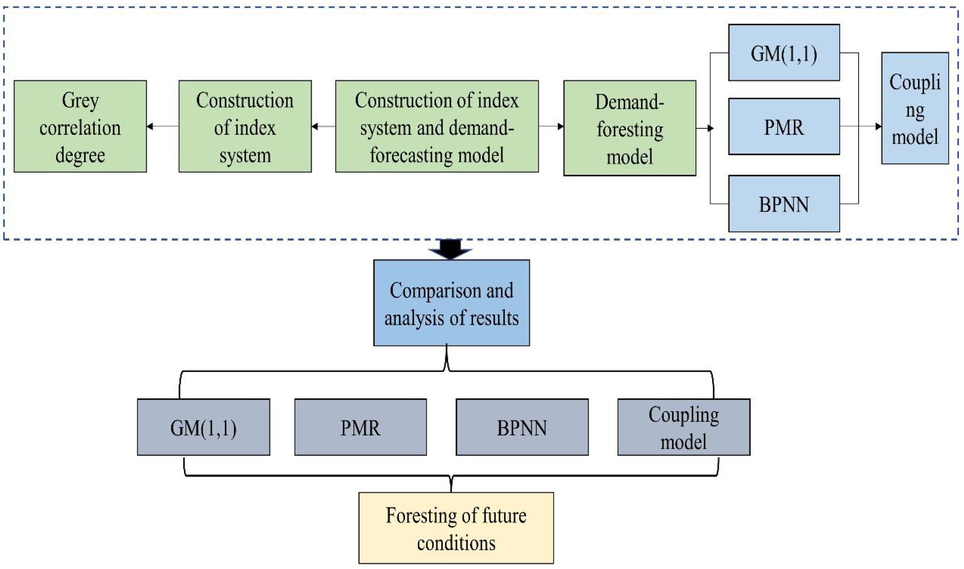
Figure 1. Workflow of study.

2. Relevant technologies

2.1. GM (1,1)

Assuming original series $X^{\left(0\right)}=\left[x^{\left(0\right)}\left(1\right)\mathrm{,}{x}^{\left(0\right)}\left(2\right)\mathrm{,}\dots \mathrm{,}{x}^{\left(0\right)}\left(n\right)\right],x^{\left(0\right)}\left(t\right)\ge 0,t=1,2,\dots ,n$ . The original sequence $X^{\left(1\right)}$ is generated into a new sequence by weighted critical value, and the following result is obtained:

$\begin{array}{ll}{X}^{\left(1\right)}=\left[x^{\left(1\right)}\left(1\right)\mathrm{,}{x}^{\left(1\right)}\left(2\right)\mathrm{,}\dots \mathrm{,}{x}^{\left(1\right)}\left(n\right)\right],t=1,2,\dots ,n& (1)\end{array}$

$\begin{array}{ll}{Z}^{\left(1\right)}\left(t\right)=\partial x^{\left(1\right)}+\left(1-\partial \right)x^{\left(1\right)}\left(t-1\right),t=1,2,\dots ,n& (2)\end{array}$

Gray differential equation of series:

$\begin{array}{ll}d\left(t\right)+\partial z\left(1\right)\left(t\right)=\gamma & (3)\end{array}$

Where $\partial$and $\gamma$ are coefficients, they are calculated by the least square method. The time response function can be obtained by solving the model:

$\begin{array}{ll}\hat{X}\left(1\right)\left(t+1\right)=\left[x^{\left(0\right)}\left(1\right)-\frac{\gamma }{\partial }\right]e^{-\partial t}+\frac{\gamma }{\partial },t=1,2,\dots ,n& (4)\end{array}$

Restore forecast to:

$\begin{array}{ll}\hat{X}\left(0\right)\left(t+1\right)=\hat{X}\left(1\right)\left(t+1\right)-\hat{X}\left(1\right)\left(t\right)=\left(1-e^{\partial }\right)\left(X\left(0\right)\left(1\right)-\frac{\gamma }{\partial }\right)e^{-\partial t}& (5)\end{array}$

The predicted value is calculated from the above calculation results, and then the development gray number and residual test are carried out for the predicted value. The residual test is as follows:

$\begin{array}{ll}\hat{E}\left(0\right)\left(i\right)=x^{\left(0\right)}\left(t\right)-\hat{X}\left(0\right)\left(t\right)& (6)\end{array}$

$\begin{array}{ll}\epsilon \left(t\right)=\frac{x^{\left(0\right)}\left(t\right)-\hat{X}\left(0\right)\left(t\right)}{x^{\left(0\right)}\left(t\right)},n=1,2,\dots ,n& (7)\end{array}$

$\begin{array}{ll}p\left(k\right)=1-\frac{1-0.5\partial }{1+0.5\partial }\lambda \left(t\right)& (8)\end{array}$

Where $\hat{E}\left(0\right)\left(i\right)$ is absolute error; $\epsilon \left(t\right)$ is relative residual error, when the absolute value of $\epsilon \left(t\right)$ is less than 0.2, the results passed the test, if it <0.1, the results are highly confident; $p\left(k\right)$ is grade ratio deviation, if the absolute value of $p\left(k\right)$ is less than 0.1, the results are highly confident.

2.2. BP neural network model

A BP (back-propogation) neural network is a hierarchical network system, which consists of three parts, including an input layer, a hidden layer, and an output layer (Guowei et al., 2023). In the process of learning, information can be transmitted in the forward direction while error can be transmitted in the reverse direction, and each layer can also be interconnected with each other. The acceptance of information can be determined by the connection weight of the network (Wan and Yu, 2023). The specific workflow is: the neurons in the input layer acquire the signal from the outside and receive it, and then transmit it to the hidden layer. The intermediate layer processes and converts the signal, then the signal is processed and transmitted to the output layer, and finally, the output layer gives the output result. At this time, a complete forward propagation is completed, but there will be errors between the output result and the actual value; so start to carry out back-propagation, the error is transferred from the output layer to the hidden layer, and then returned to the input layer for level-by-level correction (Zhang et al., 2021). The repeated application of this process can continuously reduce the error, and finally, produce an output value with relatively little error. A BP neural network also contains hidden layer nodes, and it needs to select one layer or two layers, or multiple layers according to its own data, and there is no coupling relationship between nodes at the same layer (Wang et al., 2022). The following figure shows the structure of a three-layer BP neural network.

2.3. Principle multiple linear regression model

Principal component analysis is used for dimensionality reduction. This article constructs an indicator system through principal component analysis. First, the original data is standardized. Second, the correlation coefficient matrix, eigenvalues, eigenvectors, and variance contribution rate are calculated, and eigenvalues>80% selected. Finally, the component matrix is obtained, and the matrix is normalized and orthogonal. The principal component expression is shown in equation (9):

$\begin{array}{ll}F=Z{X}_1+Z{X}_2+\dots +Z{X}_9& (9)\end{array}$

Through multiple linear regression between the principal component F and the normalized Y, we can obtain:

$\begin{array}{ll}ZY={\alpha }_1{F}_1+\dots +{\alpha }_0& (10)\end{array}$

After standardized processing:

$\begin{array}{ll}Y={\beta }_1{X}_1+{\beta }_2{X}_2+\dots +{\beta }_0& (11)\end{array}$

We finally can get the forest.

2.4. Coupling forecasting model based on Shapley value (coupling model)

Each model has its own applicable conditions and advantages and disadvantages. For the same forecasting demand, there are differences in accuracy (Wang et al., 2021). Therefore, combined forecasting becomes a good method because it can integrate the advantages of each forecasting model and try to avoid situations with large errors, so as to improve the overall accuracy and improve the forecasting effect (QHwan et al., 2023). The combination forecasting model in this paper mainly applies the linear combination method to calculate the weight of each model method, and it should be weighted according to the prediction error. The larger the error, the smaller the weight should be. This method can improve the accuracy of the forecasting model (Anderson et al., 2023; Meng et al., 2023).

The method used in this paper to calculate the weight is the Shapley value method, which is first used to solve the problem of benefit distribution, which can better achieve balanced distribution and reasonable distribution according to their respective contributions so that all members can achieve the most satisfaction. Shapley value error distribution formula is:

$\begin{array}{ll}{E}_i^{\prime }={{\displaystyle \sum }_{}}_{S\in S_i}w\left|S\right|\left(E\left(s\right)-E\left(s\right)\backslash i\right),i=1,2,\dots ,n& (12)\end{array}$

Where $w\left|S\right|=\frac{\left(n-\left|s\right|\right)!\left(\left|s\right|-1\right)}{n!}$ , which is the marginal contribution rate of portfolio members, i is ith model, $E_i^{\prime }$ is allocation error, s represents containing combinations of forecast models, $\left|s\right|$ is the number of single prediction models in the combination, $s\backslash i$ is the models excluding i in s, n is the number of prediction models in combination. And then, the weight is calculated as follows:

$\begin{array}{ll}{\mu }_i=\frac{1}{n-1}\times \frac{E-E_i}{E}& (13)\end{array}$

Where E is sharing the value of total error in combined forecasting, ${\mu }_i$ is the weight of each single forecast model.

After the weights are calculated through the above steps, the combined forecasting model is established:

$\begin{array}{ll}\widehat{Y_1}={\mu }_1\widehat{Y_{1j}}+{\mu }_2\widehat{Y_{2j}}+{\mu }_3\widehat{Y_{3j}}& (14)\end{array}$

Where $\widehat{Y_j}$ is predictive value in jth time, ${\mu }_1$ is weight number of GM(1,1), ${\mu }_2$ is the weight number of the PMR model, ${\mu }_3$ is the proportion of the BP neural network (BPNN) model, $\stackrel{}{{\widehat{Y}}_{1j}}$ is predictive value in the jth year in GM(1,1), $\stackrel{}{{\widehat{Y}}_{2j}}$ is predictive value in the jth year in the PMR model, $\stackrel{}{{\widehat{Y}}_{3j}}$ is predictive value in the jth year in the BPNN model.

3. Data description

The data in this paper are directly quoted or indirectly calculated according to the data of Yantai Port and its direct hinterland cities in relevant websites such as Yantai Statistical Yearbook, Yantai City Economic and Social Development Statistical Bulletin, China CCL Development Report, China Logistics Development Report, China Logistics Yearbook, etc. from 2010 to 2022, and due to the lack of some data, The method used in this paper is to use SPSS software to select the function of data substitution to fill in the missing values. In addition, since China’s CCL has had official statistics since 2010, the time period selected in this paper is 2010–2022.

Considering that the demand for CCL of aquatic products in all kinds of statistical reports refers to the scalar, the demand for CCL of aquatic products selected in this paper refers to the consumption of permanent residents in the immediate hinterland. Considering that the main consumers of aquatic products in Yantai Port and the hinterland cities are permanent residents, comprehensive data is available, Therefore, this paper uses (per capita consumption of aquatic products by urban residents * per capita consumption of aquatic products by urban residents + per capita consumption of aquatic products by rural residents * per capita consumption of aquatic products by rural residents) as the CCL demand of aquatic products for the permanent residents in Yantai Port and its hinterland.

The indicators of non-quantifiable influencing factors include personnel quality, government macro-policies, and regional advantages, technology. The quantifiable influencing factors include the economic environment, per capita GDP, the proportion of the tertiary industry structure, per capita disposable income, the consumer price index of aquatic products, logistics capacity, freight volume, freight turnover, port cargo throughput, human factors, per capita consumption expenditure, population, supply factors, cold chain technology, cold storage capacity, and CCL circulation efficiency.

In order to make the selected indicators have a relatively obvious impact on the logistics demand of aquatic products cold chain, the above quantifiable indicators and non-quantifiable indicators are first analyzed by gray relational analysis to get Table 1.

TABLE 1

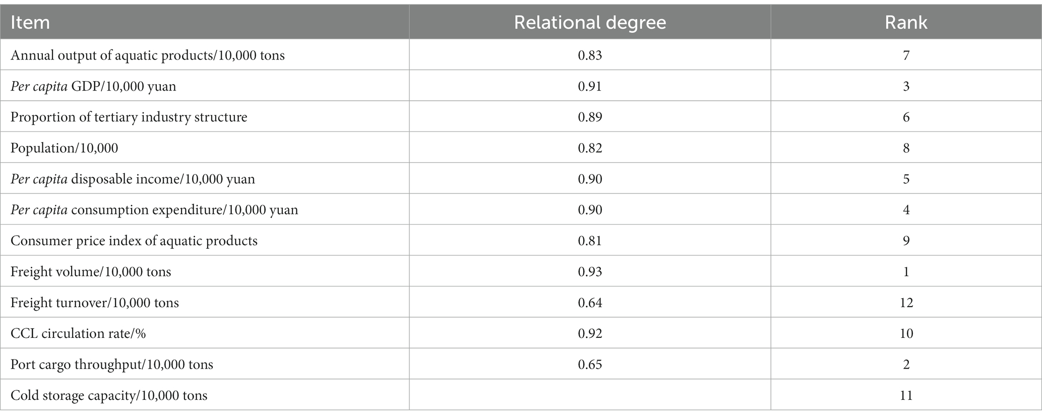
Table 1. Gray relational degree of the cold chain.

Because the value of the correlation degree is above [0.1], and the value of the correlation degree is closer to 1, the greater the influence of the dependent variable is High; selected indicators are usually greater than 0.8. From Table 1, we can see that there are 9 indicators greater than 0.8 among the 12 indicators, so we select these 9 indicators as the influencing factors to explore in this paper.

4. Results and discussion

4.1. Construction of indices system

Each factor can affect the CCL demand. When a factor changes, the CCL demand will change accordingly. At the same time, when the CCL demand changes, it will also affect some factors. Therefore, the impact factors and the demand for aquatic products are bidirectional and interactive. The correlation degree can also reflect the correlation of variables. Because many factors will have an impact on the CCL demand, it is not comprehensive to predict it based on a single variable, so it is important to predict the CCL demand based on all selected independent variables. Therefore, this paper constructs the influencing factor system of CCL demand through the combination of qualitative and quantitative methods, that is, the selection index system, as shown in Table 2.

TABLE 2

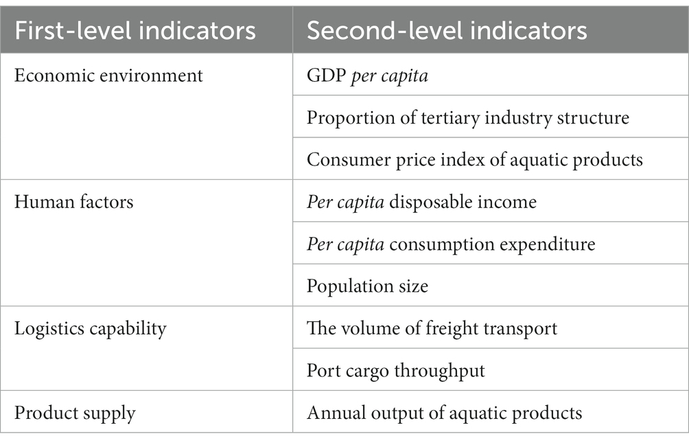
Table 2. Indices system.

The above indicator sets are named as follows: GDP per capita is X₁, the proportion of tertiary industry structure is X₂, the per capita disposable income is X₃, the per capita consumption expenditure is X₄, the consumer price index of aquatic products is X₅, the freight volume is X₆, the port cargo throughput is X₇, the annual output of aquatic products is X₈, and the population is X₉. The original data of each influencing factor index is shown in Table 3 below.

TABLE 3

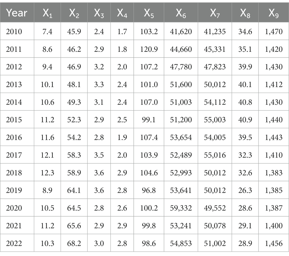
Table 3. Data description of influence factors.

4.2. Performance of models

GM(1,1) model construction results are shown in Table 4. We can see that by developing coefficient $\partial$ , posterior difference ratio C value and gray action $\gamma$ are obtained, posterior difference ratio C 0.34 < 0.35, which means that the performance of GM(1,1) is relatively good. We finally get the gray prediction model shown in equation (15).

$\begin{array}{ll}{X}^{\left(1\right)}\left(t+1\right)=\left(18.1+806.1\right){\exp }^{0.023t}-806.1& (15)\end{array}$

TABLE 4

Table 4. Comparison between the predicted value and absolute error of a single prediction model.

According to the gray prediction model, we can obtain the predictive value after inputting the original data (Figure 2).

FIGURE 2

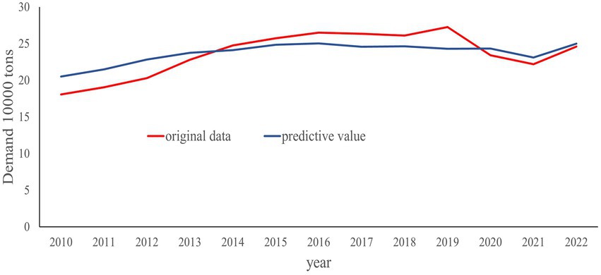
Figure 2. Fitting diagram of principal component regression prediction.

We use the historical data from 2010 to 2022 and analyze the demand from 2010 to 2022 in combination with the influencing factors mentioned above. The group data is divided into two groups, the first 8 groups are used as training data, and the last 3 groups are test data for fitting analysis. First, we will introduce the raw data, take the influencing factors as the input samples, take the consumption as the output data, and normalize the raw data. Through 10-fold cross-validation and network search test, it can be determined that when the learning efficiency is 0.1 and the maximum number of iterations is 60, the model effect reaches the best. The network structure obtained is: there are 12 neurons in the input layer, 1 neuron in the output layer, and the number of nodes in the middle two hidden layers is 8 and 5, respectively. The fitting effect is shown in Figure 3.

FIGURE 3

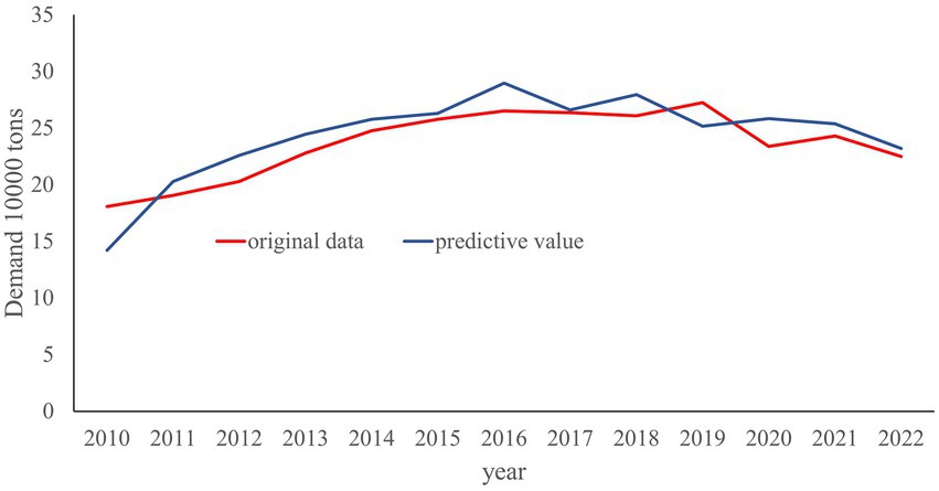
Figure 3. Fitting diagram of BP neural network.

In a comprehensive way, the research results of CCL demand forecast of aquatic products from 2010 to 2022 are analyzed, as shown in Table 4.

We can see from Table 4 that the total error sharing value of the combined forecasting model is 1.2, model set of combined forecasting I = {1, 2, 3}. According to Shapley’s relevant theory and formula, the subset error of the combined model is shown in Table 5.

TABLE 5

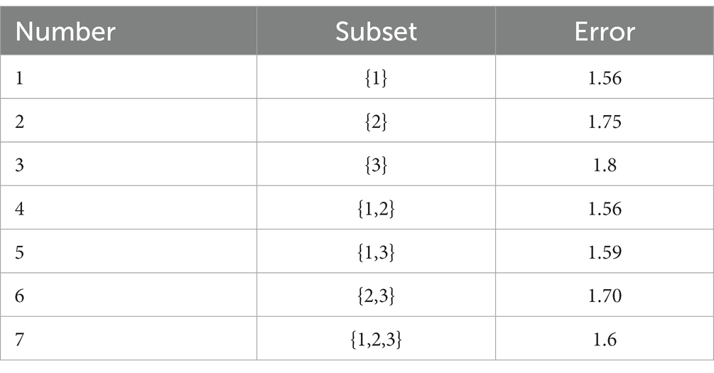
Table 5. Subset error of combined prediction model.

According to equation (12), the error amount shared by each model in the combined forecast is 0.4,0.58,0.65, respectively. The weight is 0.38,0.32,0.30, respectively. Thus it can be seen, ${\mu }_1+{\mu }_2+{\mu }_3=1$ , because the average absolute error of GM (1,1) is the smallest, the weight should be the largest, and the average absolute error of the BP neural network is the largest, so the weight should be the smallest, which is also consistent with the specific performance of Shapley value. The above weight is substituted into equation (14), and the formula of the combined prediction model is as follows:

$\begin{array}{ll}\widehat{Y_j}=0.38\widehat{Y_{1j}}+0.32\widehat{Y_{2j}}+0.30\widehat{Y_{3j}}& (16)\end{array}$

Thus, we can obtain the predictive value for the combined model Shapely-based in Figure 4.

FIGURE 4

Figure 4. Combination prediction fitting diagram.

From the perspective of the consumption of aquatic products from 2010 to 2022, there will be a significant decline in 2020. We believe that the impact of COVID-19 will be greater in 2020. At the beginning of 2020, because of the epidemic, Chinese consumers began to isolate themselves at home, and even daily necessities such as vegetables were purchased by community volunteers, so the demand for aquatic products decreased. In the later stage, cold-chain food or packaging was frequently detected positive for nucleic acid, and Yantai also had local cases due to cold-chain, which undoubtedly affected people’s purchase of cold-chain products, resulting in a downward trend in the actual demand for aquatic products in 2020. As can be seen from Figure 5, the predicted value will show an upward trend in 2020. This is because the prediction is based on most data trends, and the impact of this public health emergency cannot be considered, so the error generated is relatively large.

FIGURE 5

Figure 5. Comparison of results of the four prediction models. GM (1,1) and principle regression model (PMR) (A), BP neural network (BPNN), and coupling model (B).

We compared the absolute error and relative error of three single prediction models and combined prediction models, and the details are presented in Figure 5.

The results of each prediction model are different. Compared with the results of a single prediction model, it is found that the average relative error of BP neural network prediction is the largest. The author believes that BP neural network needs a lot of data. According to the availability of data, this paper can only select data from 2010 to 2022, so the data volume is relatively small and there is a large error; the smallest error is from the GM (1,1) model. Comparing the combined forecast with the single forecast result, it is found that the average relative error of the combined forecast result is the smallest, which also confirms the advantages of the combined forecast model, because it can combine the advantages of each model to correct the larger error, making the forecast result more stable. According to the average absolute error of the prediction value, it can also be seen that the prediction result in a single prediction model is greater than the prediction result error of the combined prediction. To sum up, each model has advantages and disadvantages. The combined forecasting model can give full play to their advantages, avoid disadvantages, reduce errors, and make the forecasting results more accurate.

4.3. Future tendency predictions

According to GM (1,1) prediction, combined with trend extrapolation, the independent variables are predicted. First, take 2010–2022 as the self-measure, take each influencing factor as the dependent variable, establish the model, carry out curve fitting, find out the method to determine the maximum square of the coefficient, write the curve fitting expression, and calculate the result. We compare the predicted value with the actual value and select the predicted value with the minimum average relative error. Combined with the characteristics of each influencing factor, the relative error of the predicted value of 2010–2022 is obtained, as shown in Table 6.

TABLE 6

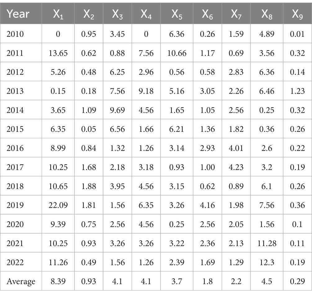
Table 6. Relative errors of independent variables (%).

It can be seen from Table 6 that the average relative error of each influencing factor index is small, so the data is meaningful and the model is applicable. The average relative error of X1 is the largest, and the GM (1,1) model is used. Considering the practical significance of the influencing factors, the trend extrapolation method is used for curve fitting, although the error is small, it is predicted that X1 will have a negative value in 2023–2027, so this model is abandoned and the GM (1,1) model is selected. Use this method to predict each influencing factor index in 2023–2027. The predicted values are shown in Table 7.

TABLE 7

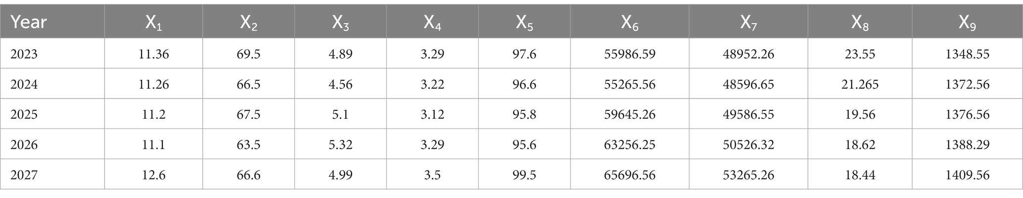
Table 7. Predicted values of independent variables 2023–2027.

The predicted values of the factors affecting the demand for CCL of aquatic products in Table 7 are substituted into three single prediction models and combined prediction models respectively, and the results are shown in Figure 6.

FIGURE 6

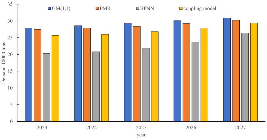
Figure 6. Comparison of forecast results of aquatic product CCL demand in 2023–2027.

We have carried out a correlation analysis on the forecast value of 2023–2027, and also selected the demand as the reference sequence. The comparison index is the X₁−X₉ we explored above. Table 8 shows the gray correlation between the demand for aquatic CCL in Yantai from 2023 to 2027 and each index.

TABLE 8

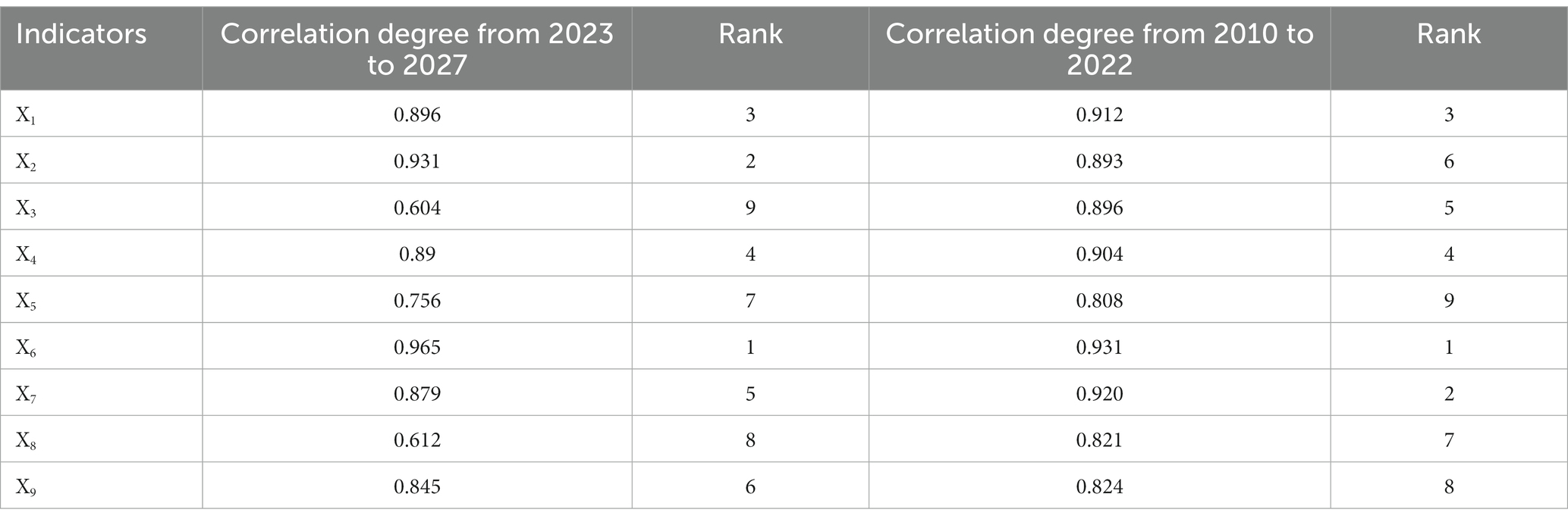
Table 8. Gray correlation degree between the demand for cold chain and indicators.

According to the prediction results (Figure 6), the CCL demand for aquatic products is gradually increasing, which also indicates that the CCL is further developing.

To sum up, it can be seen that the correlation degree of X₆ cargo volume in 2010–2022 is the same as that in 2023–2027, both ranking first, which indicates that this indicator is the most important factor affecting the logistics demand of Yantai aquatic products cold chain. In the next few years, the X₂ third industrial structure proportion ranks second in terms of relevance. According to historical data, the third industrial structure proportion ranks sixth, and the ranking has improved. The third industrial structure has also increased from 64.4% in 2020 to 72.6% in 2027, with a growth rate of 12.7%. This indicates that the gradual increase of the third industrial structure proportion in the future will drive the demand for CCL of Yantai aquatic products and promote the economic development of Yantai, the increase in demand for CCL of aquatic products will also adjust the structural proportion of the tertiary industry. The development of modern e-commerce and logistics has driven tertiary industry.

X₁ GDP per capita has a great impact on the CCL of aquatic products in the current economic society and the future economic development, and the ranking of correlation has not changed, both ranking third. It can be found that the per capita GDP has also been declining in the past 2 years. According to records, the proportion of industry in the economic structure of Yantai was very high, but with the transformation of the economic structure, the government proposed a new idea of “partial withdrawal, reduction and improvement, and green development,” and reduced the capacity of industrial steel. Yantai also has corresponding countermeasures to create a civilized city, so these will have an impact on the GDP. The consumption expenditure per capita of X₄ ranks fourth. According to the data, consumption expenditure per capita has been on the rise. The purchasing power of residents has improved, the number of aquatic products purchased is more, and the demand for aquatic products is higher. X₃ The per capita disposable income dropped from the fifth to the ninth. The main reason is that when per capita disposable income reaches a certain level, a further increase will not increase the demand for aquatic products. After all, aquatic products are not necessities. If the price of aquatic products rises, it may even reduce the demand for them.

The X₅ aquatic product consumer price index shows a downward trend in the future forecast, and the correlation degree rises from the 9th to the 7th. This indicator refers to that when the retail price of aquatic products changes, the actual living expenses of residents will be affected, because as the price rises, the actual living expenses will inevitably increase, and the corresponding consumer price index will show a downward trend, which can indirectly reflect the changes in the price of aquatic products, When the price rises, residents’ willingness to buy decreases, thus reducing demand.

X₈ annual output of aquatic products. From 2010 to 2014, the annual output of aquatic products increased year by year. In recent years, the development of the cold chain has been in an orderly manner. Farmers seize the opportunity to increase the scale of production and aquaculture. From 2014 to 2020, the annual output of aquatic products showed a downward trend. According to the trend, the output of aquatic products decreased. According to the principle of supply and demand balance, the price of aquatic products will increase, which will naturally affect the demand for aquatic products. The correlation degree of X₉ population index increased from 8 to 6, and its impact on the cold chain demand of aquatic products gradually increased. Therefore, the positive role of population is increasing.

The correlation degree of cargo throughput of X₇ port has dropped from the second to the fifth, with a large range of decline. As a port city, Yantai must consider the cargo handling capacity of the port, expand the port transport scale, improve transport efficiency, and reduce losses and waste.

As far as the current development is concerned, the support of the national and provincial governments has a strong supporting role in the development of CCL. The improvement of various transportation and other infrastructure will also greatly promote local development in the future. Under the existing conditions, we should give full play to the greatest advantages of existing resources and try to improve the deficiencies. Yantai CCL will continue to develop rapidly.

4.4. A comparison with others

In order to verify the robustness of the coupling model we proposed, we compared the results of our method with that of other machine learning methods in cold chain demand, details see Table 9.

TABLE 9

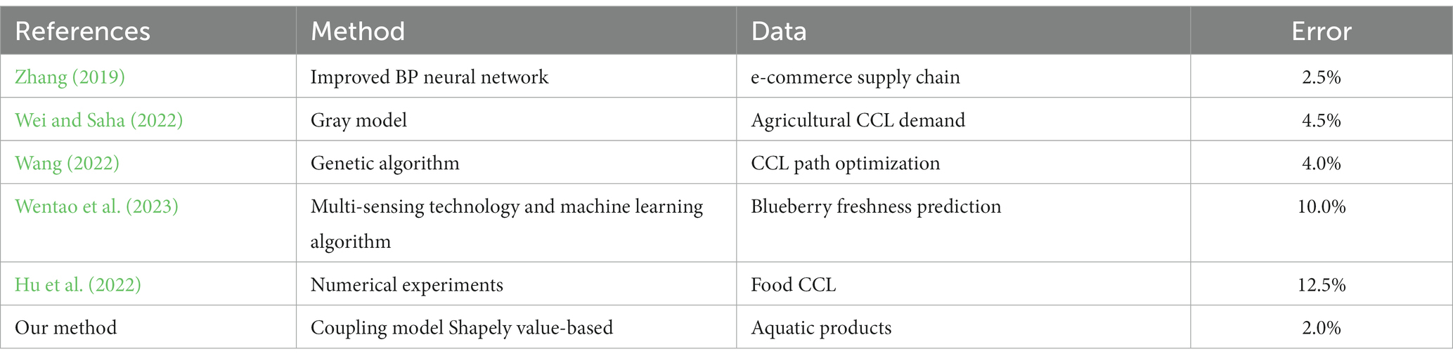
Table 9. Comparative analysis between our method and others in CCL prediction.

As shown in Table 9, our method, i.e., coupling model Shapely value-based, can improve substantially the accuracy in predictions of CCL. For example, Ren et al. (Wei and Saha, 2022) used the gray model GM (1, N) with fractional order accumulation to forecast future agricultural CCL demand in Beijing, Tianjin, and Hebei, they found that agricultural cold chain demand in Beijing and Hebei will grow sustainably in 2021–2025, while the trend in Tianjin remains stable. However, the methods still need to be improved compared to our methods, our methods may provide a reference for improving accuracy. The accuracy of our method is approximate to the results of Zhang (2019), who proposed an optimized BP neural network to predict aquatic product export volume with a low error of 2.5%. Which means that our method is highly robust. Notably, our method is more convenient in its application, as in Zhang Yizhuo’s study, complex algorithms were used to optimize the parameters. However, we only combined the traditional model (gray model, principle component regression model, and BP neural network model) through the Shapely value, which is a relatively easy process compared to Zhang’s, and the accuracy of our method is a little higher than Zhang’s (98% vs. 97.5%).

4.5. Limitations

From the economic perspective, the per capita GDP of Yantai Port and its immediate hinterland has shown a downward trend in the past 2 years, the economic development speed has slowed down, and the annual output of aquatic products has also shown a downward trend in the past 2 years. According to the forecast results, the per capita GDP has shown an upward trend, but the increase is not large, and the annual output of aquatic products has shown a downward trend (Nianxin et al., 2022; Mojtaba and Hossein, 2023; Yuanjie et al., 2023). This shows that the economic development of Yantai Port and its hinterland city, Yantai City, is slow and the output is declining.

In the logistics capacity, cargo volume and port cargo throughput play an important role in the development of CCL (Qian et al., 2022). According to the data from 2010 to 2015, the freight volume showed a growth trend, and the increase and decrease of the freight volume from 2015 to 2020 showed an interactive change, and the difference between 2020 and 2015 was small. The predicted freight volume increased but only returned to the state before the decline. The port cargo throughput has not increased in the past 4 years. In general, the logistics capacity is slightly insufficient (Shen et al., 2022).

From the perspective of humanity, the population has slowed down in recent years. The population has increased in the forecast, but it has not reached the number in 2011. This will lead to the loss of talent to a certain extent, and reduce the number of professionals in the CCL industry (Ning et al., 2022). Cold chain technology. According to the original data, the circulation rate of CCL in Yantai Port and its hinterland cities is relatively low, and there is a large gap between the circulation rate of CCL and that of the country. The freezing, cold storage, ice making, and other capabilities need to be improved (Chen et al., 2022).

Therefore, it should increase the policy support of aquatic products, increase the annual output of aquatic products, and improve the economic level of the hinterland; improve port infrastructure construction, accelerate intelligent construction, increase CCL capacity, improve the level of information technology, improve the innovation ability and increase the talent introduction policy, increase the construction of green energy-saving cold storage, and improve cold chain technology.

In addition, because the traditional machine learning regression model has the assumption that the samples are independent and irrelevant, it cannot consider the information of the time sequence, and cannot carry out end-to-end multi-step time series prediction. In the future, we can introduce the cyclic neural network to solve the above drawbacks, but the simple cyclic neural network cannot remember too much information in its history when the time series is relatively long. A deep learning algorithm based on Seq2Seq + Attention is needed to solve the problem of end-to-end time series multi-step prediction. Specifically, first of all, in terms of data processing, we can identify historical sales outliers based on Huber Loss’s linear regression method; Secondly, in the aspect of feature extraction, commodity embedding vector representation based on Pearson correlation coefficient; Finally, in terms of prediction algorithm, a deep learning algorithm based on Seq2Seq + Attention is proposed to solve the problem of end-to-end time series multi-step prediction.

5. Conclusion

According to the principle of availability of indicators selected, the initial indicators are selected, and the indicators with higher impact on the CCL demand of aquatic products are calculated and selected by using the gray correlation degree, namely, indicators greater than 0.8. Finally, 9 indicators are selected as the independent variables of this study, and the indicator system is established. Compare the prediction model, and select the single prediction model and the combination prediction model. The single prediction model includes the gray GM (1,1) model, the prediction model combined with principal component and regression analysis, the BPNN model, and the coupling model is established through the Shapley value method. The data indicators from 2010 to 2022 are selected for example analysis, and the final results show that the combined forecasting accuracy is high. Through the combination of trend extrapolation method and time series method, the independent variables of 2023–2027 are predicted. Through the above prediction model, the combined prediction model is selected to predict the logistics demand of aquatic products cold chain from 2023 to 2027. The analysis results show that the predicted logistics demand shows an upward trend, and the future aquatic products CCL has great power and development prospects. According to the results and trend analysis, the limitations of the development of aquatic CCL in Yantai Port and its hinterland cities are found, and corresponding countermeasures and suggestions are put forward.

Data availability statement

The raw data supporting the conclusions of this article will be made available by the authors, without undue reservation.

Author contributions

SH: conceptualization, supervision, methodology, and project administration. XS: investigation, resources, and writing—original draft preparation. SH and XS: data curation, validation, and writing—review and editing. All authors contributed to the article and approved the submitted version.

Funding

The study was funded by Henan University of Animal Husbandry and Economy, Doctoral Research Startup Fund of Henan University of Animal Husbandry and Economy (project no.: 2020HNUAHEDF039), Ministry of Education of China, Humanities and Social Sciences, Youth Fund projects (project no.: 22YJC630106) and The Education Department of Henan Province, Research project of Humanities and Social Sciences in Colleges and Universities of Henan Province (project no.: 2023-ZDJH-034).

Conflict of interest

The authors declare that the research was conducted in the absence of any commercial or financial relationships that could be construed as a potential conflict of interest.

Publisher’s note

All claims expressed in this article are solely those of the authors and do not necessarily represent those of their affiliated organizations, or those of the publisher, the editors and the reviewers. Any product that may be evaluated in this article, or claim that may be made by its manufacturer, is not guaranteed or endorsed by the publisher.

References

Abad, E., De Zarate, A. G. L., Gomez, J. M., Juarros, A., Marco, S., and Nuin, M. (2009). RFID smart tag for traceability and cold chain monitoring of foods: demonstration in an intercontinental fresh fish logistic chain. J. Food Eng. 8, 393–394. doi: 10.1016/j.jfoodeng.2009.02.004

CrossRef Full Text | Google Scholar

Abada, P. L., and Vijay, A. (2005). Incorporating transport cost, in the lot size and pricing decisions with downward sloping demand. Int. J. Product Econ. 95, 297–305. doi: 10.1016/j.ijpe.2006.04.016

CrossRef Full Text | Google Scholar

Abimannan, A., Spiros, P., and Sadayan, P. (2023). Biogenic amines in fresh fish and fishery products and emerging control. Aquacult. Fisher 8, 431–450. doi: 10.1016/J.AAF.2021.02.001

CrossRef Full Text | Google Scholar

Alasali, F., Nusair, K., Alhmoud, L., and Zarour, E. (2021). Impact of the COVID-19 pandemic on electricity demand and load forecasting. Sustainability 13:1435. doi: 10.3390/su13031435

CrossRef Full Text | Google Scholar

Anderson, N., Sharan, R., Martin, D., and Beyerlein Irene, J. (2023). A machine learning model to predict yield surfaces from crystal plasticity simulations. Int. J. Plast. :161. doi: 10.1016/J.IJPLAS.2022.103507

CrossRef Full Text | Google Scholar

Antón, R. P., Martín, L. N., and Juan, P. A. J. (2021). Systematic review of electricity demand forecast using ANN-based machine learning algorithms. Sensors 21:4544. doi: 10.3390/S21134544

PubMed Abstract | CrossRef Full Text | Google Scholar

Casado-Vara, R., Martin del Rey, A., Pérez-Palau, D., de-la-Fuente-Valentín, L., and Corchado, J. M. (2021). Web traffic time series forecasting using LSTM neural networks with distributed asynchronous training. Mathematics 9:421. doi: 10.3390/math9040421

CrossRef Full Text | Google Scholar

Cefola, M., De Bonis, M. V., and Pace, B. (2016). Preliminary modeling of the visual quality of broccoli along the cold chain. Eng. Agricult. Environ. Food 10, 109–114. doi: 10.1016/j.eaef.2016.11.005

CrossRef Full Text | Google Scholar

Chen, Z., Lyu, H., Zhu, H., and Peng, J. (2022). Empirical study on the algorithms of food CCL for multi-regional and large-scale athletic sports. Int. J. Wirel. Mob. Comput. 22, 328–337. doi: 10.1504/IJWMC.2022.10049469

CrossRef Full Text | Google Scholar

Cheng, W. A. N. G. (2022). A review of research on risk assessment of fresh agricultural product supply chain. Asian Agric. Res. 14, 1–26. doi: 10.19601/j.cnki.issn1943-9903.2022.10.001

CrossRef Full Text | Google Scholar

Gharabaghi, S., Stahl, E., and Bonakdari, H. (2019). Integrated nonlinear daily water demand forecast model (case study: City of Guelph, Canada). J. Hydrol. 579:124182. doi: 10.1016/j.jhydrol.2019.124182

CrossRef Full Text | Google Scholar

Guo, X., and Wang, Y. (2012). Multi-objective model for logistics distribution programming considering logistics service level. J Southwest Jiaotong Univ 25, 874–880. doi: 10.3969/j.issn.0258-2724.2012.05.023

CrossRef Full Text | Google Scholar

Guowei, W., Jiaxin, W., Wang Jiawei, Y., and Haiye, S. Y. (2023). Study on prediction model of soil nutrient content based on optimized BP neural network model. Commun. Soil Sci. Plant Anal. 54, 463–471. doi: 10.1080/00103624.2022.2118291

CrossRef Full Text | Google Scholar

Han, Z., Hua, L., Fang, Y., Ma, Q., Li, Y., and Wang, J. X.. Innovative research on refrigeration technology of cold chain logistics (2020). In: IOP Conference Series: Earth and Environmental Science, 474(5): 052105.

Google Scholar

Hu, Y., Zhang, R., Qie, X., and Zhang, X. (2022). Research on coal demand forecast and carbon emission reduction in Shanxi Province under the vision of carbon peak. Frontiers in Environmental Science 2022:923670. doi: 10.3389/FENVS.2022.923670

CrossRef Full Text | Google Scholar

Hofman, W. J. (2000). “Information and communication Technology for Food and Agribusiness Chain management in agribusiness and the food industry,” in Proceedings of the fourth. international conference. 2000, 599–608.

Google Scholar

Julia, B., JensPeter, L., and Karen, J. S. (2016) Characteristics of Demand Structure and Preferences for Wild and Farmed Seafood in Germany. Marine Resource Economics. 31, 281–300.

Google Scholar

Karim, N., Kennedy, T., Linton, M., Watson, S., Gault, N., and Patterson, M. (2011). Effect of high pressure processing on the quality of herring and haddock stored on ice. Food Control 22, 476–484. doi: 10.1016/j.foodcont.2010.09.030

CrossRef Full Text | Google Scholar

Kim, K., Kim, H., Kim, S.-K., and Jung, J.-Y. (2016). I -RM: an intelligent risk management framework for context-aware ubiquitous CCL. Expert Syst. Appl. 46, 463–473. doi: 10.1016/j.eswa.2015.11.005

CrossRef Full Text | Google Scholar

Liu, M.-L., and Yang, B.-C. (2018). Study on cold chain technology investment decision of dual channel aquatic supply chain under the background of Hayes road. Eur. Bus. Manage 4:80. doi: 10.11648/j.ebm.20180403.13

CrossRef Full Text | Google Scholar

Meng, J., Qiu, P. C., Jian, L., LiGang, X., and Li, L. C. (2023). Explainable machine learning model for predicting furosemide responsiveness in patients with oliguric acute kidney injury. Ren. Fail. 45:2151468. doi: 10.1080/0886022X.2022.2151468

CrossRef Full Text | Google Scholar

Mojtaba, S. S., and Hossein, K. M. (2023). Utilization of unconventional water resources (UWRs) for aquaculture development in arid and semi-arid regions – a review. Ann. Anim. Sci. 23, 11–23. doi: 10.2478/AOAS-2022-0069

CrossRef Full Text | Google Scholar

Nianxin, Z., Xinna, L., Kaimin, P., Hui, C., Min, Y., Ye Tai, W., et al. (2022). A novel aptamer-imprinted polymer-based electrochemical biosensor for the detection of Lead in aquatic products. Molecules 28:196. doi: 10.3390/MOLECULES28010196

PubMed Abstract | CrossRef Full Text | Google Scholar

Ning, X., Tian, W., He, F., Bai, X., Sun, L., and Li, W. (2022). Hyper-sausage coverage function neuron model and learning algorithm for image classi cation. Pattern Recogn. 136:109216. doi: 10.1016/j.patcog.2022.109216

CrossRef Full Text | Google Scholar

QHwan, K., Sunghee, L., Ami, M., Jaeyoon, K., Hyeon-Kyun, N., Baik, C. K., et al. (2023). A simulation physics-guided neural network for predicting semiconductor structure with few experimental data. Solid State Electron. 201:108568. doi: 10.1016/J.SSE.2022.108568

CrossRef Full Text | Google Scholar

Qian, C., Jianping, Q., Yang Han, W., and Wenbin, A. (2022). Sustainable food CCL: from microenvironmental monitoring to global impact. Compr. Rev. Food Sci. Food Saf. 21, 4189–4209. doi: 10.1111/1541-4337.13014

CrossRef Full Text | Google Scholar

Shen, L., Yang, Q., Yunxia, H., and Jinglin, L. (2022). Research on information sharing incentive mechanism of China's port CCL enterprises based on blockchain. Ocean Coast. Manag. 225:179. doi: 10.1016/J.OCECOAMAN.2022.106229

CrossRef Full Text | Google Scholar

Tarantilis, C. D., and Kiranoudis, C. T. (2002). Distribution of fresh meat. J. Food Eng. 51, 85–91. doi: 10.1016/S0260-8774(01)00040-1

CrossRef Full Text | Google Scholar

Taylor, Q., Usher, J., and Roberts, J. (2001). Foresting freight demand using economic indices. Int. J. Phys. Distribut. Logist. Manage. 31:229. doi: 10.1108/09600030210430660

CrossRef Full Text | Google Scholar

Wan, J., and Yu, B. (2023). Early warning of enterprise financial risk based on improved BP neural network model in low-carbon economy. Front. Energy Res 10. doi: 10.3389/FENRG.2022.1087526

CrossRef Full Text | Google Scholar

Wang, J. (2022). Optimization of CCL distribution path based on genetic algorithm. Acad J. Comput. Informat. Sci. 5. doi: 10.25236/AJCIS.2022.051315

CrossRef Full Text | Google Scholar

Wang, Z., and Bessler, D. A. (2002). The homogeneity restriction and forecasting performance of VAR-type demand systems: an empirical examination of US meat consumption. J. Forecast. 21, 193–206. doi: 10.1002/for.820

CrossRef Full Text | Google Scholar

Wang, C., Ning, X., Sun, L., Zhang, L., Li, W., and Bai, X. (2022). Learning discriminative features by covering local geometric space for point cloud analysis, In: IEEE transactions on geoscience and remote sensing.

Google Scholar

Wang, C., Wang, X., Zhang, J., Zhang, L., Bai, X., Ning, X., et al. (2021). Uncertainty estimation for stereo matching based on evidential deep learning. Pattern Recogn. 124:108498. doi: 10.1016/j.patcog.2021.108498

CrossRef Full Text | Google Scholar

Wei, X., and Saha, D. KNEW: key generation using NEural networks from wireless channels [C]. In: Proceedings of the 2022 ACM Workshop on Wireless Security and Machine Learning. (2022): 45–50.

Google Scholar

Wentao, H., Xuepei, W., Junchang, Z., Jie, X., and Xiaoshuan, Z. (2023). Improvement of blueberry freshness prediction based on machine learning and multi-source sensing in the CCL. Food Control 145:109496. doi: 10.1016/J.FOODCONT.2022.109496

CrossRef Full Text | Google Scholar

Xiaofeng, X., Yi, Z., Shihua, Z., Xiaoqiang, Z., and Xuelai, Z. (2023). Preparation and heat transfer model of stereotyped phase change materials suitable for CCL. J Energ Storage 60:106610. doi: 10.1016/J.EST.2023.106610

CrossRef Full Text | Google Scholar

Yang, D. (2020). Logistics demand forecast model for port import and export in coastal area. J. Coast. Res. 103, 678–681. doi: 10.2112/SI103-138.1

CrossRef Full Text | Google Scholar

Yuanjie, T., Zhenni, W., Shaohua, Z., Xin, L., and Yinxin, C. (2023). Identification of antibiotic residues in aquatic products with surface-enhanced Raman scattering powered by 1-D convolutional neural networks. Spectrochim. Acta A Mol. Biomol. Spectrosc. 289:122195. doi: 10.1016/J.SAA.2022.122195

PubMed Abstract | CrossRef Full Text | Google Scholar

Yun, S. Y., Namkoong, S., Rho, J. H., Shin, S. W., and Choi, J. U. (1998). A performance evaluation of neural network models in traffic volume forecasting. Mathemat. Comput Model. 27, 293–310. doi: 10.1016/S0895-7177(98)00065-X

CrossRef Full Text | Google Scholar

Zhang, Y. (2019). Application of improved BP neural network based on e-commerce supply chain network data in the forecast of aquatic product export volume. Cogn. Syst. Res. 57, 228–235. doi: 10.1016/j.cogsys.2018.10.025

CrossRef Full Text | Google Scholar

Zhang, J., Jiong, Z., Zongguo, Z., and Yue, L. (1648). Collection and application of intelligent technical information data of CCL of aquatic products (2020). J. Phys. Conf. Ser. 1648:042038. doi: 10.1088/1742-6596/1648/4/042038

CrossRef Full Text | Google Scholar

Zhang, L., Sun, L., Li, W., Zhang, J., Cai, W., Cheng, C., et al. (2021). A joint Bayesian framework based on partial least squares discriminant analysis for finger vein recognition. IEEE Sensors J. 22, 785–794. doi: 10.1109/JSEN.2021.3130951

CrossRef Full Text | Google Scholar

Zheng, R., Xiaorong, X., Xing, J., Cheng, H., Zhang, S., Shen, J., et al. (2020). Quality evaluation and characterization of specific spoilage organisms of Spanish mackerel by high-throughput sequencing during 0 °C cold chain logistics. Foods 9:312. doi: 10.3390/foods9030312

PubMed Abstract | CrossRef Full Text | Google Scholar

Zhi, H., Yunrui, F., Linhui, H., Ma, Q., Xing, W. J., and Gao, J. (2020). Research on the development of CCL of aquatic products in Zhoushan of China. In: IOP Conference Series: Materials Science and Engineering, 787.

Google Scholar