Relationship between plant species diversity and aboveground biomass in alpine grasslands on the Qinghai–Tibet Plateau: Spatial patterns and the factors driving them

Alpine grasslands are important ecosystems on the Qinghai–Tibet Plateau and are extremely sensitive to climate change. However, the spatial responses of plant species diversity and biomass in alpine grasslands to environmental factors under the background of global climate change have not been thoroughly characterized. In this study, a random forest model was constructed using grassland ground monitoring data with satellite remote sensing data and environmental variables to characterize the plant species diversity and aboveground biomass of grasslands in the Three-River Headwaters Region within the Qinghai–Tibet Plateau and analyze spatial variation in the relationship between the plant species diversity and aboveground biomass and their driving factors. The results show that (1) the selection of characteristic variables can effectively improve the accuracy of random forest models. The stepwise regression variable selection method was the most effective approach, with an R² of 0.60 for the plant species diversity prediction model and 0.55 for the aboveground biomass prediction model, (2) The spatial distribution patterns of the plant species diversity and aboveground biomass in the study area were similar, they were both high in the southeast and low in the northwest and gradually decreased from east to west. The relationship between the plant species diversity and aboveground biomass varied spatially, they were mostly positively correlated (67.63%), but they were negatively correlated in areas with low and high values of plant species diversity and aboveground biomass, and (3) Analysis with geodetector revealed that longitude, average annual precipitation, and elevation were the main factors driving variation in the plant species diversity and aboveground biomass relationship. We characterized plant species diversity and aboveground biomass, as well as their spatial relationships, over a large spatial scale. Our data will aid biodiversity monitoring and grassland conservation management, as well as future studies aimed at clarifying the relationship between biodiversity and ecosystem functions.

1. Introduction

The relationship between species diversity and productivity has been the subject of much debate (Waide et al., 1999; Adler et al., 2011; Grace et al., 2016; Chen et al., 2018). Biodiversity is concerned with the stability and sustainability of ecosystem functions and affects the value of ecosystem services and regional quality development (Bai et al., 2004). In large-scale grassland ecosystems, there is great spatial heterogeneity in species composition and productivity due to variation in geography, climate, and other environmental conditions; consequently, the relationship between species diversity and productivity can vary. Single-peaked patterns, positive correlations, and negative correlations have been observed, and the lack of a correlation between species diversity and productivity has also been observed (Ma and Fang, 2006; Adler et al., 2011). At the regional scale, enhancing the monitoring and assessment of grassland biodiversity and ecosystem functions is essential for the development of grassland biodiversity conservation policies and grassland ecosystem management.

Remote sensing technology has a wide monitoring range and can be used to monitor vegetation over long periods unlike traditional ground survey approaches, it has thus been widely used to monitor variables such as grassland aboveground biomass (AGB) and plant species diversity (PSD) (Reddy et al., 2021; Ge et al., 2022; Sun et al., 2022). Indicators such as grassland biomass and plant species richness are well correlated with remotely sensed vegetation indices such as the normalized vegetation index (NDVI) and enhanced vegetation index (EVI), and they are often used to construct grassland models (Oindo and Skidmore, 2002; Chitale et al., 2019; Reddy, 2021; Yu et al., 2021). Due to the large area and diversity in grassland types, spatial heterogeneity in grasslands is pronounced, and multiple environmental variables need to be integrated to construct high-precision models. In previous studies in which biomass has been monitored via remote sensing, several variables including vegetation indices, climate, topography, soil, and other variables have been used to increase model accuracy (Liang et al., 2016). However, few studies have integrated variables such as effective vegetation index, climate, topography, soil, and other variables into models for large-scale grassland species diversity monitoring (Choe et al., 2021; Zhao et al., 2022). In addition, some studies (Fauvel et al., 2020; Ge et al., 2022) have compared the efficacy of multiple machine learning models for modeling grassland species diversity and biomass, previous studies have shown that the random forest (RF) model is particularly effective. However, the inclusion of various environmental variables can increase model complexity, multicollinearity of the model can also affect model accuracy. Consequently, the selection of key variables is critical for enhancing the computational efficiency and accuracy of models (Zeng et al., 2019; Yu et al., 2021). Screening for effective variables can improve the computational efficiency of models and reduce the workload of model spatial simulations.

Study of the spatial relationship between plant species diversity and aboveground biomass (PSD–AGB) in grasslands, as well as the mechanisms driving it is important for enhancing our understanding of grasslands and promoting their conservation. Some researchers have analyzed the PSD–AGB relationship in local areas using field data (Waide et al., 1999; Zhu et al., 2017; Sakowska et al., 2019), and some valuable insights have been obtained. But these studies have been limited to small spatial scales based on ground survey data. However, the PSD–AGB relationship varies with the spatial scale of the study (Chase and Leibold, 2002), Ni et al. (2007) showed that the PSD–AGB relationship varies at different ecological scales and geographic scales. Previous studies have been limited by the inability to achieve large scale PSD and AGB, so the PSD–AGB relationship at large scales is still inadequate, while the current remote sensing-based technology can provide high precision estimation of PSD and AGB at the large scales (Choe et al., 2021; Wang et al., 2022), which providing us with the possibility to study the spatial relationship between the two. In addition, the relationship between species diversity and biomass is not only influenced by multiple environmental factors but also by spatial factors (Spyros Tsiftsis, 2018; Li et al., 2020; Du et al., 2022; Ma et al., 2022). Qi et al. (2022) showed that the relationship between species diversity and biomass in the Qinghai–Tibetan Plateau was generally nonlinear and positive over space, and Omidipour et al. (2021) showed that the relationship between species diversity and biomass differed among grassland areas. But in study areas with large environmental differences, it is well worthwhile to deeply investigate how the PSD–AGB relationship in large scale grasslands, and what environmental factors drive spatial distribution patterns.

The Qinghai–Tibet Plateau features typical alpine grassland ecosystems, there is wide spatial variation in vegetation growth, and this region is highly sensitive to climate change (Ma et al., 2017; Piao et al., 2019). Therefore, several environmental variables need to be considered to efficiently monitor spatial patterns of and correlations between grassland species diversity and their productivity functions, as well as the response of grassland ecosystems to global climate change, this information can also aid ecological conservation efforts. In this study, grassland species richness and above-ground biomass data obtained from ground-based surveys, along with satellite remote sensing data, were used to analyze spatial relationships between species diversity and productivity and their drivers in alpine grasslands of the Qinghai–Tibet Plateau. The specific objectives were to (1) establish a reliable model to estimate the spatial distribution of species diversity and grassland productivity in the study area; (2) analyze spatial patterns in correlations between grassland species diversity and productivity in the study area; and (3) explore the main factors driving the spatial relationships between grassland species diversity and productivity in the study area.

2. Materials and methods

2.1. Study area

Our study was conducted in the Three-River Headwaters Region in the eastern part of the Qinghai–Tibet Plateau. The Three-River Headwaters Region is located in southern Qinghai Province, China from 31°39′N to 36°16′N and from 89°24′E to 102°41′E. The average elevation of the region is above 4,000 m, the average annual temperature ranges from −5.4 to 6.9°C, the average annual precipitation ranges from 392 to 764 nm, and the total area of the study area is 395,000 km². The sources of the Yangtze River, Yellow River, and Lancang River are located in the Three-River Headwaters Region, this region is also the world’s highest and largest plateau wetland area and the most biodiversity high-altitude area, it is thus often referred to as the “Chinese Water Tower,” “Plateau Species Gene Bank,” and the “gene pool of plateau species” (Zhao, 2021). In addition, 71% of the region comprises typical alpine grassland ecosystems, the main types of grasslands are alpine meadows, alpine grasslands, and temperate grasslands. These grasslands provide several extremely important ecosystem services for the region, such as water containment, climate regulation, biodiversity maintenance, and a pasture supply.

2.2. PSD and AGB ground monitoring data

We collected field data during the peak of the grassland growing season from July to August 2021. In the field survey, 429 sample plots were set up to cover all grassland types in the study area as far as possible, with a relatively uniform spatial distribution and easy accessibility (Figure 1). In order to match with modis pixels, we set the sample plot size to 250 m × 250 m, and investigated the information of centroid coordinates, grassland vegetation types within the sample plot. Three to five replicate quadrats were set up in each sample plot, and the quadrat size was 1 m × 1 m. To collected information on the longitude (X), latitude (Y) and elevation of each quadrat, as well as the vegetation species richness, cover and height of the grassland community within the quadrat. The species richness was determined by counting the total number of species present within the quadrat. The vegetation cover was visually estimated by determining the percentage of the quadrat area covered by the vertical projection of the vegetation. The vegetation in the quadrats was mowed, bagged, taken to the laboratory, dried in an oven at 65°C for 48 h, and weighed to obtain the dry weight of grass biomass. To match quadrat-scale data to the sample plot scale, we took the average species richness and biomass dry weight of all quadrats in each sample plot to represent the PSD and AGB of that sample plot. A total of 417 valid sample plot data were obtained using the sample data set.

FIGURE 1

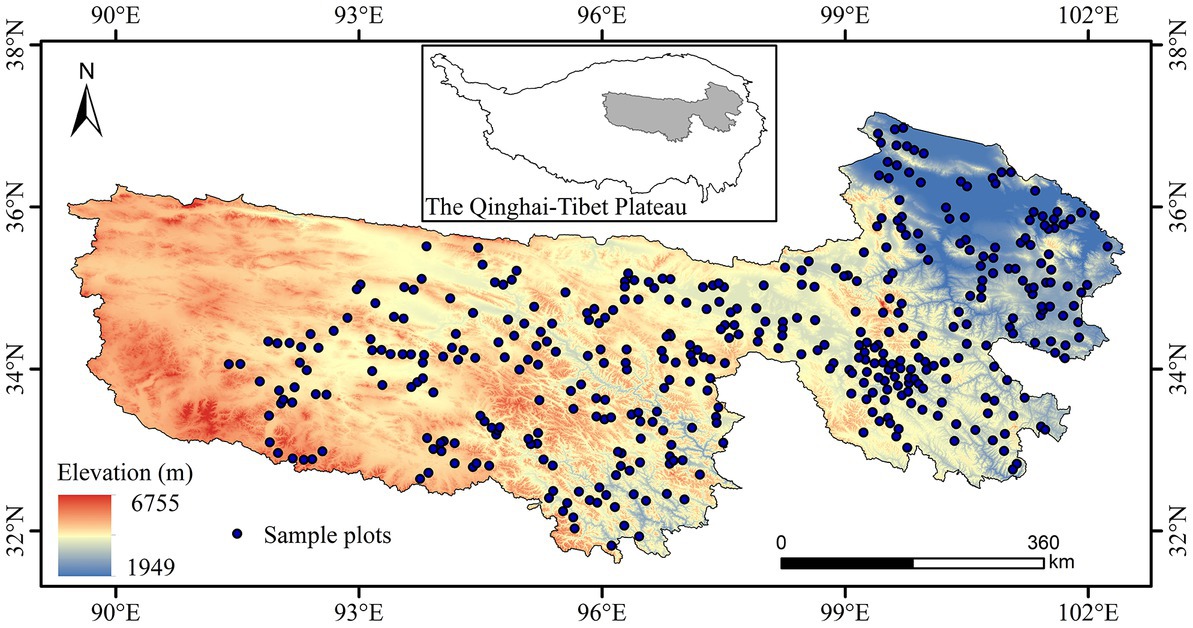
Figure 1. Location of the study area and spatial distribution of sample plots.

2.3. Remote sensing vegetation index

The satellite remote sensing data were called MOD09Q1 data and obtained using the Google Earth Engine (GEE) platform with a spatial resolution of 250 m and a temporal resolution of 8 d. The entire coverage of the study area required three scenes of images(h24v05, h25v05, and h26v05), and a total of 15 remote sensing images were obtained throughout the field survey (July 27 to August 24). A total of five vegetation indices, normalized vegetation index (NDVI), enhanced Vegetation Index 2 (EVI2), ratio vegetation index (RVI), soil adjustment vegetation index (SAVI), and optimization of soil-adjusted vegetation index (OSAVI), were calculated and downloaded through the GEE platform editor. The vegetation indices of each sample plot were extracted separately using ArcGIS software.

2.4. Data on other variables

Digital elevation model (DEM) data were obtained from Space Shuttle Radar Topography Mission (SRTM) images with a spatial resolution of 30 m and a spatial reference of GCS_WGS_1984. Slope gradient (SLOPE) and slope orientation (ASPECT) data with a resolution of 30 m were generated using ArcGIS software.

The National Geoscience Data Center¹ application was used to obtain month-by-month precipitation, temperature, and potential evapotranspiration data for 2021 with a spatial resolution of 1 km. The data were converted from nc format to tiff format in ArcGIS software, and the average values for the 12 months were used to calculate annual mean temperature (MAT), mean annual precipitation (MAP), and mean annual potential evapotranspiration (SPEI). The averages for May to October were used as the mean growing season temperature (MGT), mean precipitation (MGP), and mean potential evapotranspiration (GSPEI) in the study area.

Soil data were obtained from the National Geoscience Data Center (see text footnote 1) in nc format with a spatial fraction of 1 km. The data included soil bulk weight (BD), sand content (SA) chalk content (SI), clay content (CL), soil organic matter (SOM), total nitrogen content (TN), and total phosphorus content (TP) for eight soil layers at a depth of 0 to 3 m. Due to the relatively shallow root system of the grasslands, soil data from a depth of 0 to 0.3 m in the soil surface layer were used.

Grassland spatial distribution data were extracted from the secondary classification by downloading the LUCC2020 surface classification data. These grassland cover data in the study were extracted by masking the vector boundary of the Three-River Headwaters Region and these data were used to mask the grassland boundary in the study area.

We resampled the above data (DEM, SLOPE, ASPECT, MAT, MAP, SPEI, MGT, MGP, GSPEI, BD, SA, SI, CL, SOM, TN, and TP) at different resolutions to 250 m, the grassland boundary in the study area was then masked to extract the sample data for analysis.

2.5. PSD and AGB modeling inversion methods

2.5.1. Variable filtering methods

We prepared sample site latitude and longitude, five remotely sensed vegetation indices, and 16 environmental variables for a total of 23 variable factors to construct grassland PSD and AGB models. The complexity of the model increases with the number of variables included, variable screening can eliminate the problem of multicollinearity between multiple variables to improve model accuracy and computational efficiency. Thus, the selection of variables appropriate for machine learning modeling is key.

In this study, two methods, stepwise regression (STEP) and least absolute shrinkage and selection operator (LASSO), were used to determine the optimal set of variables and the optimal model. The STEP model works by introducing variables one by one into the model. STEP eliminates insignificant variables so that the multicollinearity between the retained variables is reduced, thus ensures that the final set of explanatory variables chosen by the model is optimal. LASSO (Wang et al., 2008) can deal with multicollinearity by automatically selecting the most important independent variables and setting the values of less important predictor variables to zero, thereby only retaining the most useful features. Both variable selection methods were implemented in RStudio, STEP was conducted through a stepwise fitting function, and LASSO was conducted through the “glmnet” package.

2.5.2. RF model construction and accuracy verification

In this study, PSD and AGB regression models for grasslands were established using the RF model. The models used the measured PSD and AGB data as dependent variables, and the variables obtained from the above 23 variables, as well as the variables identified from the STEP and LASSO variable selection methods, as independent variables. A total of six models were established, and the accuracy of the models was evaluated using the PSD and AGB data to identify the optimal variable screening results and models.

RF is a novel nonparametric machine learning algorithm that uses multiple decision trees to train samples and integrate predictions (Li, 2019). We incorporated all the independent and dependent variables into 417 datasets according to their spatial location, and randomly selected 293 sample plot data points (70% of valid samples) from the datasets as training datasets and 124 sample plot data points (30% of valid samples) as test datasets in the RF modeling process. In this study, the RF algorithm was implemented using the “randomForest” package in RStudio, and the optimal model was obtained by adjusting the number of decision classification trees (ntree) and the number of features of node segmentation (mtry) to find the optimal model. The model accuracy was evaluated using three metrics: root mean square error (RMSE), correlation coefficient (R²), and mean absolute error (MAE). The formulas used to calculate these metrics are as follows:

$\begin{array}{ll}RMSE=\sqrt{\frac{{\displaystyle \sum }_{i=1}^n{\left(y_i-\widehat{y_i}\right)}^2}{n}}& (1)\end{array}$

$\begin{array}{ll}{R}^2=1-\frac{{\displaystyle \sum }_{i=1}^n{\left(y_i-\widehat{y_i}\right)}^2}{{\displaystyle \sum }_{i=1}^n{\left(y_i-\overline{y_i}\right)}^2}& (2)\end{array}$

$\begin{array}{ll}MAE=\frac{1}{n}{\displaystyle \sum }_{i=1}^n\left|y_i-\widehat{y_i}\right|& (3)\end{array}$

where n is the number of sample plots, $y_i$ is the model predicted value of the ith sample plot, $\overline{y_i}$ is the measured value of the ith sample plot, and $\widehat{y_i}$ is the average of the measured values.

2.6. PSD and AGB correlation analysis method

Traditional raster data correlation analysis can only be used to calculate the correlation coefficients between two variables; however, this approach cannot be used to characterize the spatial distribution of correlations between raster data pixel-by-pixel. Consequently, we used a 3 × 3 moving window (nine pixels in each window) for the two raster data sets, the correlation coefficient of each spatially corresponding window was determined, and the spatial distribution of the correlations between the two raster data pixels was determined. The spatial distribution of the image-by-image correlations of raster data was finally obtained. The spatial distribution of the PSD–AGB relationship was obtained using the above method to analyze the pixel-by-pixel correlation of the PSD and AGB rasters.

2.7. Determination of the factors driving variation in the dependent variables

We used geodetector (Wang and Xu, 2017) to detect spatial heterogeneity, which mainly includes factor detectors, interaction detectors, risk detectors, and ecological detectors. Factor detectors are mainly used to detect the degree to which the independent variable X explains spatial heterogeneity in the dependent variable Y, and interaction detectors are used to detect the degree to which the interaction between two independent variables explains spatial heterogeneity in the dependent variable Y. The principle can be summarized as follows.

$\begin{array}{ll}q=1-\frac{1}{N{\sigma }^2}\sum N_h{\sigma }_h^2& (4)\end{array}$

where q is an indicator of spatial heterogeneity; ${\sigma }^2$ is the variance of the variable; h is the stratification of the variable, and the value of q ranges from 0 to 1. Larger q values indicate stronger explanatory power of the variable.

In this study, a total of 16 geographic factors (LAT, LON, DEM, SLOPE, and ASPECT), climatic factors (MAT, MAP, and SPEI), and soil factors (BD, SA, SI, CL, SOM, TN, and TP) were used for single-factor detection and interaction detection of the spatial relationships of PSD–AGB to identify the factors driving variation in PSD–AGB. The GD package in R software was used for geodetector factor detection and interaction detection.

3. Results

3.1. Descriptive statistics of the PSD and AGB data

The descriptive statistics of PSD and AGB of the 417 measured samples used in the modeling are shown in Table 1. The maximum value of PSD was 26 n/m², the minimum value was 3 n/m², the mean value was 10.27 n/m², the standard deviation (SD) was 4.60 n/m², and the coefficient of variation (CV) was 0.45. The maximum value of AGB was 4365.70 kg/ha, the minimum value was 157.90 kg/ha, the mean value was 1465.43 kg/ha, the SD was 824.21 kg/ha, and the CV was 0.56.

TABLE 1

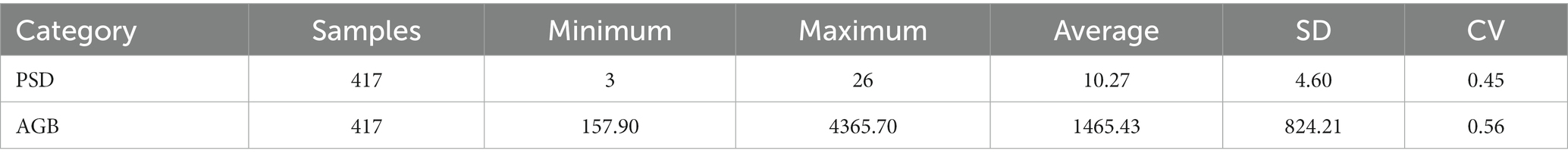
Table 1. Descriptive statistics of the PSD and AGB data of the measured grassland.

3.2. Variable selection and model accuracy evaluation

In the PSD variable screening, STEP screening yielded eight variables: X, Y, EVI2, RVI, SAVI, MAT, SPEI, and SI. LASSO screening yielded nine variables: X, Y, EVI2, RVI, SPEI, SLOPE, BD, SI, and TN. Variables selected by both variable selection results included X, Y, EVI2, RVI, SPEI, and SI6. The model built with variables based on STEP screening had the highest accuracy (R², RMSE, and MAE of the test set were 0.60, 2.92, and 2.37, respectively), followed by the model built with all variables (R², RMSE, and MAE of the test set were 0.58, 3.00, and 2.45, respectively). The R², RMSE, and MAE of the test set from the LASSO-screened variables were 0.57, 3.03, and 2.46, respectively (Table 2). According to the accuracy indicators of the model training set and test set, the RF model established by the STEP screened variables was the optimal model for PSD estimation in the study area.

TABLE 2

Table 2. Results of variable selection and evaluation of model accuracy.

STEP screening of AGB variables yielded seven variables: X, Y, EVI2, RVI, MAT, DEM, and TN. LASSO screening yielded eight variables: X, Y, NDVI, EVI2, RVI, MAT, SLOPE, and CL. According to the RF model accuracy evaluation, variable screening can improve the estimation of AGB accuracy, and the R², RMSE, and MAE of the test set from the STEP-screened variables were 0.55, 578.93, and 434.10, respectively, followed by LASSO-screened variables (R², RMSE, and MAE of 0.52, 596.51, and 450.99, respectively, for the test set) (Table 2). The RF model established by STEP screened variables was finally used for AGB estimation in the study area based on the above results.

3.3. Comparison of measured and model predicted values of PSD and AGB

Based on the optimal models of PSD and AGB, we extracted the predicted and measured values of the models in the test set and established linear relationships and value domain distribution plots to evaluate the estimation ability of the models (Figure 2). In general, there were strong linear relationships of measured values with the PSD estimation model and the AGB estimation model, the PSD estimation model explained 60% of the variation in grassland PSD, and the AGB estimation model explained 55% of the variation in grassland AGB. However, both models underestimated high values and overestimated low values. In the PSD estimation model, the median model estimate was slightly higher than the measured value overall, and the model estimates were significantly higher than measured values between 8 and 12 n/m². In the AGB estimation model, the median model estimates were slightly lower than the measured values, the model overestimates AGB near values of 1,500 kg/ha and underestimates AGB when values exceed 2,200 kg/ha.

FIGURE 2

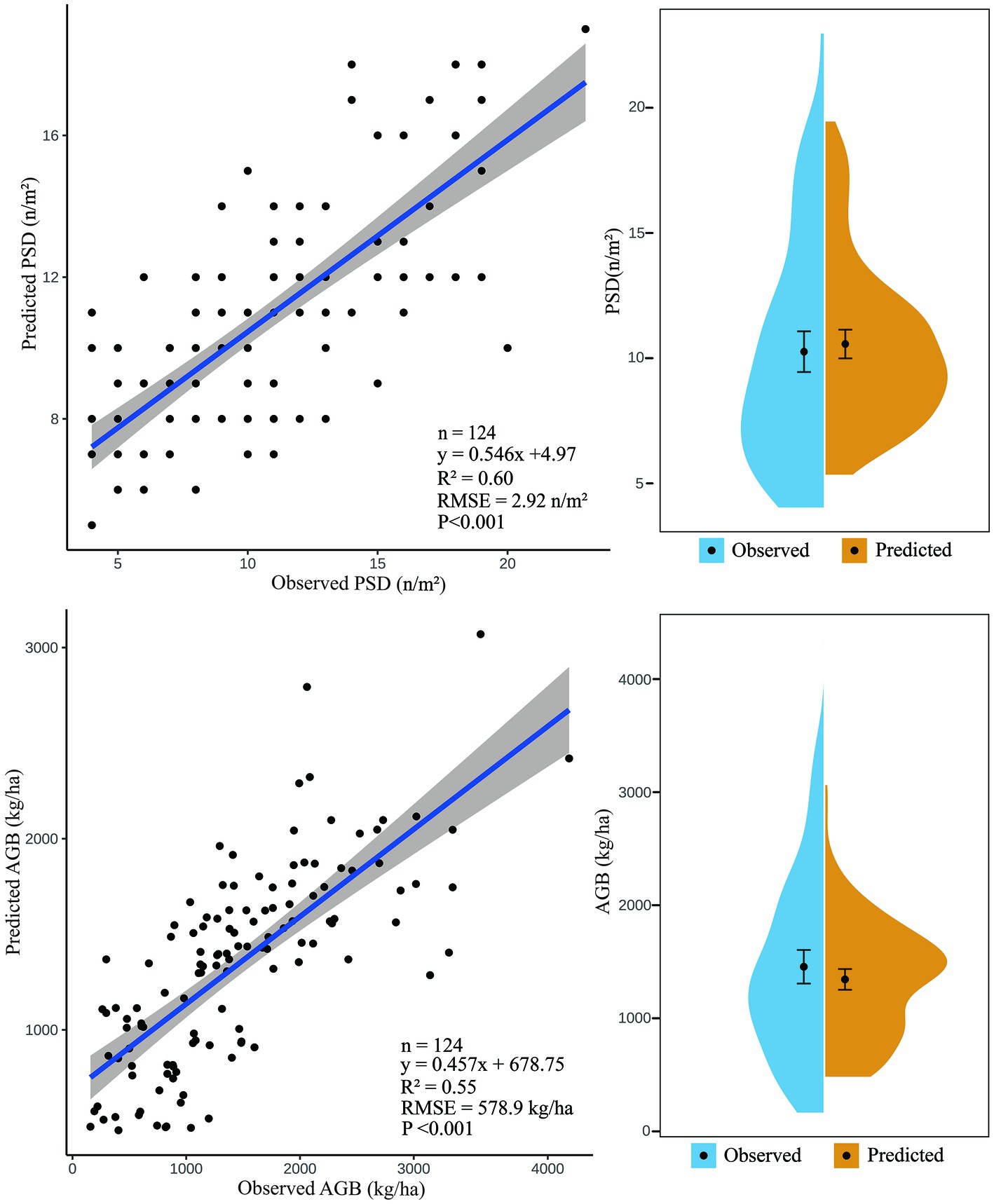
Figure 2. Comparison of the measured values of PSD and AGB with the predicted values of the optimal model.

3.4. PSD and AGB spatial distribution characteristics

We inferred the spatial distribution of the maximum PSD and AGB in the study area in 2021 using the optimal model obtained by STEP screening variables (Figure 3). In general, the spatial distribution patterns of PSD and AGB are basically similar and mainly decrease from east to west and from southeast to northwest, some differences in their distribution were also observed in local areas. PSD and AGB were high in Nangqian and Yushu in the southern Three-River Headwaters Region and Henan, Zeku, Jiuzhi, and Banma in the southeast. PSD and AGB are medium in Xinghai, Maduo, Qumalai, Zaduo, and Eastern Zhiduo. The PSD and AGB are low in western Zhiduo and Geermu. Slight spatial differences were observed between PSD and AGB in some local areas, such as northwestern Republican County where AGB is not high, but PSD is high, the same pattern was also observed in local areas in Xinghai and Zhiduo counties, as well as in local areas in Zeku, Henan, Maqin, Gande, and Jiuzhi counties where AGB is particularly high, but PSD is not particularly high. The minimum value of PSD of the inversion model in the study area was 4 n/m², the maximum value was 18 n/m², the mean value was 9.42 n/m², and the standard deviation was 2.37 n/m². The minimum value of AGB of the inversion model was 541.13 kg/ha, the maximum value was 2695.14 kg/ha, the mean value was 1392.34 kg/ha, and the standard deviation was 395.09 kg/ha.

FIGURE 3

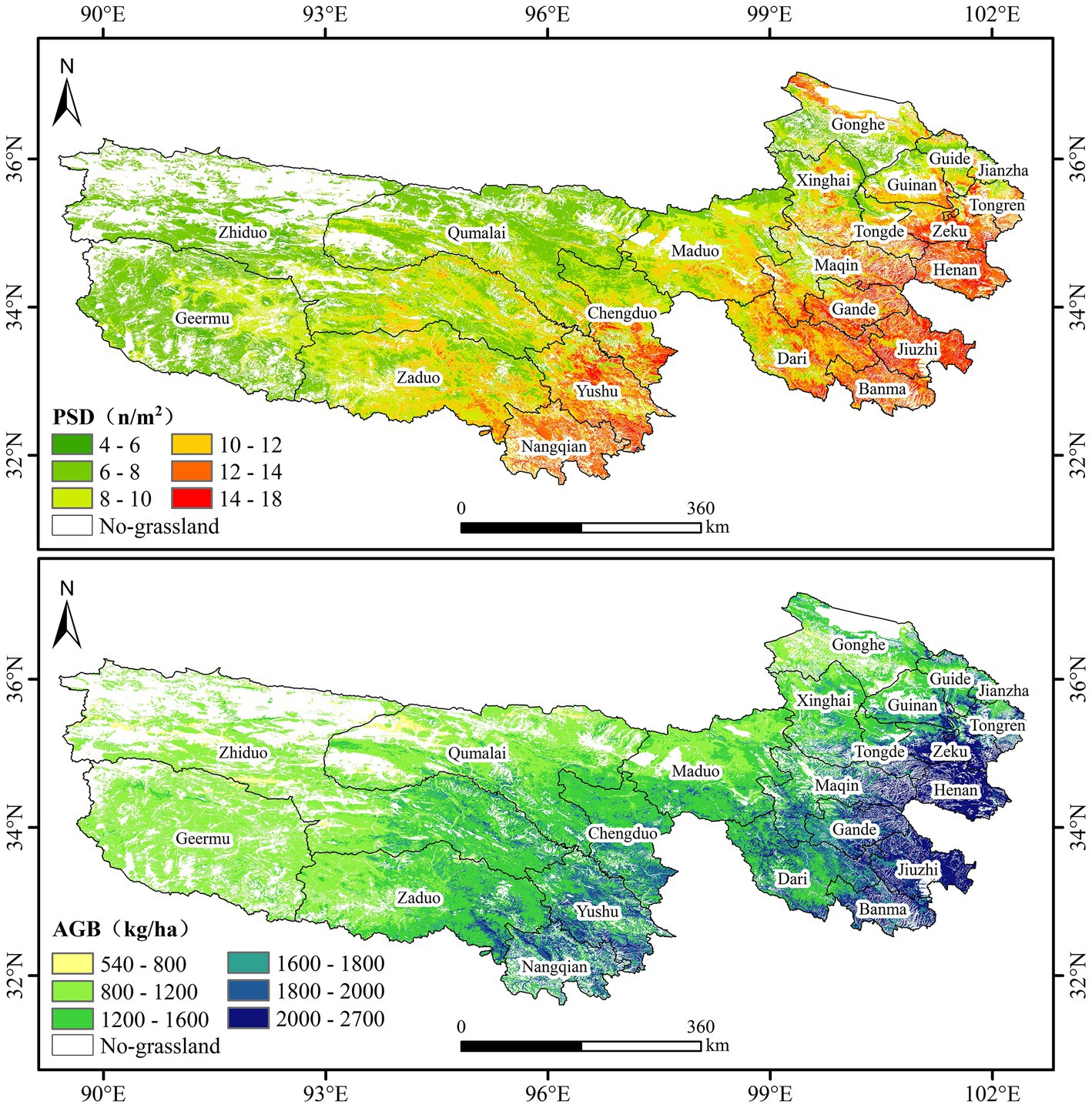
Figure 3. PSD and AGB spatial distribution map.

3.5. Spatial pattern of PSD–AGB relationships

To analyze the spatial PSD–AGB relationships in different regions, we conducted pixel-by-pixel correlation analysis of PSD and AGB and obtained the spatial pattern shown in Figure 4. Large spatial variation was observed in the PSD–AGB relationship, mostly negative correlations were observed in the northwest and southeast, and mostly positive correlations were observed in the central region. Areas with negative correlations were mainly distributed in Geermu, Western Zhiduo, and Northern Qumalai in the northwestern part of the study area and local areas in Henan, Zeku, Maqin, and Jiuzhi counties in the southeastern part of the study area. In addition, negative correlations were also observed in the Jifushan mountain range (source of the Lancang River) at the junction of Zhiduo and Zaduo and in the valley of the Yellow River Basin (upstream of Longyangxia) in eastern Xinghai County. In addition, the PSD–AGB correlation coefficient was positive and strong in the central part of the study area in Qumalai, Eastern Zhiduo, Zaduo, and Chengduo and in the northeastern part of the study area in Xinghai, Guinan, and Guide. The correlations were positive and weak in the central part of the study area in Yushu, Maduo, Dari, Gande, and Banma. According to the PSD–AGB correlation coefficient significance statistics, a significant positive correlation was observed for 39.24% of the regions in the study area (p < 0.05), non-significant positive correlations were observed for 28.39% of the regions in the study area, significant negative correlations were observed for 9.36% of the regions in the study area (p < 0.05), non-significant negative correlations were observed for 20.58% of the regions in the study area, and non-significant relationships were observed for 2.43% of the study area.

FIGURE 4

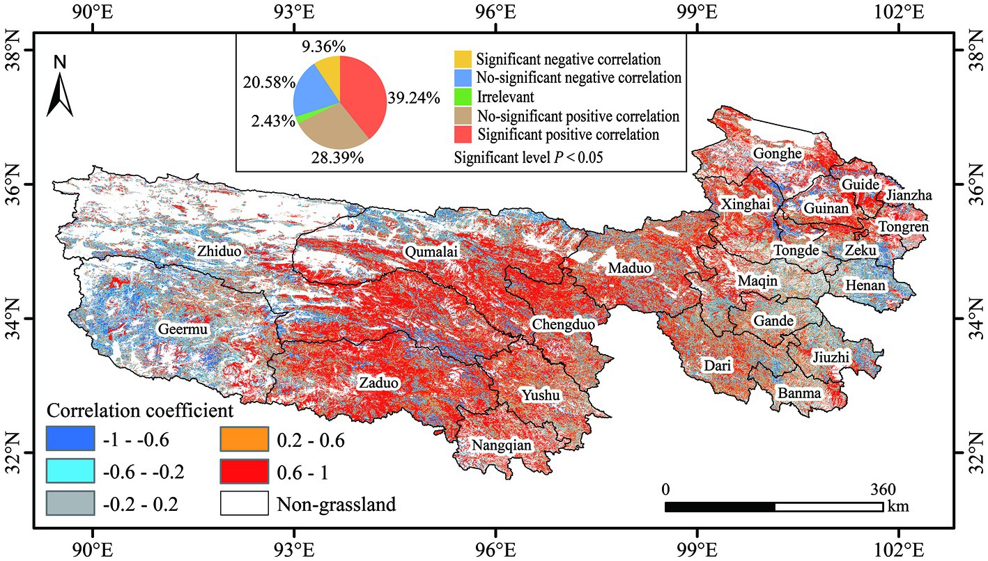
Figure 4. Spatial variation in the PSD–AGB relationship.

3.6. Factors affecting spatial variation in the PSD–AGB relationship

Based on the q-statistic values of single factors detected via the geodetector (Figure 5A), the most important factors driving spatial variation in the PSD–AGB relationship in the study area were LON, followed by MAP, DEM, SI, TP, LAT, MAT, SLOPE, BD, SPEI, SOM, TN, SA, CL, and ASPECT. The q-value of LON was the largest (0.29), followed by MAP (0.21), DEM (0.18), and SI (0.15), indicating that spatial variation in the PSD–AGB relationship in the study area was mainly affected by LON, followed by MAP, DEM, and SI. The q-values of the other factors were lower, the q-value of ASPECT was the lowest (0.01).

FIGURE 5

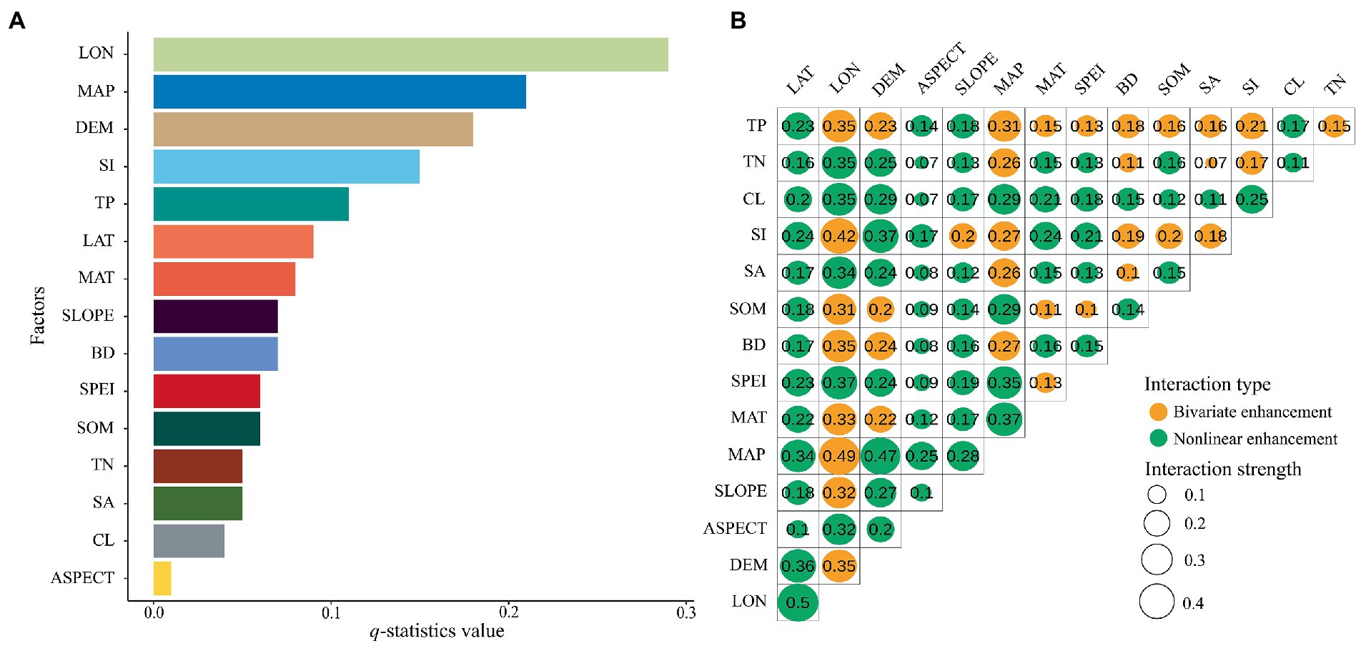
Figure 5. Value of the q-Statistic for each variable. (A) shows the univariate probes for each variable and (B) shows the interaction probes for each variable.

Interaction effects (Figure 5B) on spatial variation in the PSD–AGB relationship were stronger than the effects of any single factor, and this same finding was obtained via two-factor enhancement and nonlinear enhancement. Factors with high performance include LON, MAP, and DEM, and the strongest interaction effect was that of LON–LAT (0.5 according to the nonlinear enhancement), followed by the interactions of LON–MAP (0.49 according to two-factor enhancement) and MAP–DEM (0.47 according to nonlinear enhancement).

4. Discussion

4.1. PSD and AGB inversion model accuracy

The results of this study show that variable selection effectively improved the accuracy of both the PSD and AGB models. The accuracy of the variable model was highest according to the STEP method, which is consistent with the results of Ge et al. (2022) showing that the accuracy of the variable model was highest when the STEP method was used. Wang et al. (2022) used three variable selection methods, although they did not use the STEP method, their results show that variable selection improves model accuracy. The STEP method used in this study introduces variables into the model one by one and eliminates insignificant variables, thus ensuring that the final set of explanatory variables obtained is optimal. In light of the widespread use of machine learning, an increasing number of environmental variables have been used as independent variables in models; thus, variable selection can greatly improve the computational efficiency of the model while also improving model accuracy. Overall, the specific variable selection method that enhances model accuracy likely varies with the study objective, data source, and comparison method.

The optimal AGB model of this study had an R² of 0.55, which is less accurate than previous simulations of the AGB of grasslands in the Three-River Headwaters Region according to the studies of Liang et al. (2016) (R² of 0.701) and Wang et al. (2022) (R² of 0.60) but more accurate than the study of Wang et al. (2018) (R² of 0.31). The optimal model of Liang et al. (2016) used grassland height, which has a direct relationship with productivity; consequently, their inverse AGB accuracy is higher. However, there is still much uncertainty in the inverse of grassland height. In contrast, Wang et al. (2022) used 1,620 samples obtained over 10 years, on the one hand the sample size was larger, and on the other hand the model was trained for environmental changes over a 10 year period, so the model accuracy was higher than this study. The R² of the optimal model in this study was 0.60, and the RMSE was 1.65 n/m² in the simulation of PSD; the RMSE of the RF model in Zhao et al. (2022) was 1.94 n/m², and the RMSE of the optimal HASM-XGBoot model reached 1.19 n/m². HASM can effectively solve ecological environmental surface modeling errors, thus improving the accuracy of conventional machine learning models, we aim to test combinations of HASM methods in the future. Generally, the sample size involved in the model, the variables involved in the modeling, and modeling methods vary, and this greatly affects the accuracy of the model.

Comparison of the measured and predicted values of the two models in this study revealed that the accuracy of both models was high; however, both models underestimated high values and overestimated low values, which is a common problem of many machine learning models (Ge et al., 2022; Sabatini et al., 2022; Zhao et al., 2022). In addition, the overall fit of the PSD model was better than that of the AGB model, the model overestimated PSD when values were near 9 n/m², and the model overestimated AGB when values were near 1,500 kg/ha. This might be explained by the uneven spatial distribution of our field sampling data, the large size of the study area, the large altitudinal gradient, and the fact that the western region is mostly uninhabited because of its harsh climate. Thus, some areas with low values in the west were not considered, and areas with medium values were mainly concentrated in the center of the study area (Figure 1).

4.2. PSD and AGB spatial distribution characteristics

According to the spatial distributions of the inversion models of PSD and AGB, both PSD and AGB were high in the southeastern portion of the study region and low in the northwestern portion of the study region. The spatial distribution of AGB was similar to that observed in Zeng et al. (2019) using the RF model and Wang et al. (2018) using the ANN model; AGB values were high in southeastern portions of Henan, Zeku, Gander, and Jiuzhi and central and southern parts of Nangqian and Yushu; AGB values were lower in western regions. AGB ranged from 540 to 2,700 kg/ha in our study, which is similar to the range reported in Zeng et al. (300 to 2,500 kg/ha). The range of AGB values observed in Wang et al. (250 to 3,250 kg/ha) differed from that observed in our study, this difference might be related to differences in the variables included in the model and the methods used. The similar spatial distributions of PSD and AGB observed in our study are consistent with the hypothesis that biodiversity and productivity are positively correlated (Loreau et al., 2001); however, local differences in their distributions were observed. The PSD and AGB of species around Qinghai Lake are likely high because of the suitable water and heat conditions around the lake, but this area is traditionally used for grazing (Zhai et al., 2017), and the reason for the low AGB may be related to the high grazing intensity in the area. In addition, large-scale inverse mapping of grassland species diversity models has not been widely studied, the results of our study are superior in terms of model accuracy and spatial distribution. This method permits large-scale biodiversity remote sensing monitoring in grasslands with large heterogeneity, which fills gaps with no monitoring data in some unoccupied areas. Moreover the PSD spatial distribution map shows the spatial distribution pattern on a large scale, and these data can aid biodiversity assessment and conservation.

4.3. Spatial variation in PSD–AGB relationships and factors driving variation in PSD–AGB relationships

Recent studies that have examined PSD–AGB relationships have seldom considered the possible effects of spatial scale and spatial heterogeneity on PSD–AGB relationships. Most studies have focused exclusively on small spatial scales or regions with little spatial variation. In this study, we analyzed spatial variation in the PSD–AGB relationship on a large scale while accounting for geographical heterogeneity. Our findings indicate that the relationship between PSD and AGB in the western and southeastern parts of the study area was mostly negatively correlated, and the relationship between PSD and AGB in other regions was positively correlated. Significant positive correlations were observed over 39.24% of the study region, and significant negative correlations were observed over 9.36% of the study region. It is noteworthy that combining the spatial distribution of PSD and AGB (Figure 3), we found that PSD and AGB were negatively correlated in areas with low and high values; by contrast, PSD and AGB were positively correlated in areas with medium values. For this reason, we determined the relative contributions of various environmental factors driving spatial variation in the PSD–AGB relationship using geodetector. According to the single-factor analysis, longitude was the factor that had the largest effect on the PSD–AGB relationship (explaining 29% of the variation in the spatial pattern), followed by annual precipitation, altitude, and SI. And the factor interaction analysis revealed that longitude explained 50% of the variation in the PSD–AGB relationship; however, the interaction between precipitation, elevation, and SI had the greatest effect on spatial variation in the PSD–AGB relationship. Zhu et al. (2017) also showed that the PSD–AGB relationship varied with longitude in the Tibetan Plateau. Wang et al. (2007) and Xu et al. (2019) showed that spatial variation in the PSD–AGB relationship was correlated with longitude, latitude, and altitude. The study area spans several degrees of longitude but only a few degrees of latitude; consequently, there is large variation in longitude, as well as a significant elevational gradient and precipitation gradient in the east–west direction of the study area. Longitude, elevation, and precipitation in the east–west direction thus explain much spatial variation in the PSD–AGB relationship. Temperature varies more in the latitudinal direction, and the latitudinal variation in our study area was low, this might explain the weak effect of temperature on spatial variation in the PSD–AGB relationship. In addition, the spatial resolution of soil property data used in this study was 1 km, and spatial variation in several variables was low, this might contribute to explaining the weak effects of soil environmental variables on variation in the PSD–AGB relationship, with the exception of SI. Spatial variation in the environment of grassland plant communities can lead to differences in community characteristics and thus spatial variation in the PSD–AGB relationship. We speculate that the resource use complementarity hypothesis might explain variation in the PSD–AGB relationship across our study area (David Tilman, 1997; Loreau et al., 2001), the western part of the study area has a harsh climate, infertile soils, fewer available resources for plants, and strong interspecific competition, which results in a negative relationship between PSD and AGB. In the central part of the study area, the hydrothermal conditions are improved and the abundance of resources available to plants is greater. Increases in species diversity promote the complementary use of resources among species, which enhances the accumulation of biomass. However, PSD values plateaued in the southeastern part of the study area where biomass was highest. In addition, ecological niche space was lower, light, soil nutrients, and other resources were limited, interspecific competition was intense, and some dominant plants suppressed the growth of inferior plants in this region, such observations explain the negative relationship between PSD and AGB in areas with high AGB values (Schnitzer et al., 2011; Guo and Berry, 2013; Albert et al., 2022; Qi et al., 2022). Grassland productivity includes AGB and belowground biomass. In our study, we only monitored and analyzed the relationship between AGB and PSD. Additional monitoring of belowground biomass is needed in subsequent studies to characterize the spatial relationships between PSD and productivity.

5. Conclusion

In this study, an RF model was constructed using grassland ground monitoring data along with satellite remote sensing data and environmental variables to characterize spatial distribution patterns in PSD and AGB in the Three-River Headwaters Region. The accuracy of the model was compared using three variable selection methods, and the STEP variable selection method showed the highest performance, which indicates that variable selection could effectively improve the accuracy of the RF model. The R² of the PSD and AGB test sets based on the optimal STEP-RF model was 0.6 and 0.55, and the RMSE was 2.92 n/m² and 578.93 kg/ha, respectively. Spatial distribution patterns in PSD and AGB across the study area was similar, the PSD and AGB values were generally high in the southeast and low in the northwest. The modeling approach used in this study could be used to monitor grassland species diversity and productivity on a large scale, it could also aid biodiversity monitoring and grassland conservation management.

We also analyzed spatial variation in the PSD–AGB relationship, as well as the environmental variables driving variation in this relationship, including climate, topography, and soil. The PSD–AGB relationship tended to be mostly positively correlated. However, the PSD–AGB relationship was mostly negatively correlated in regions with low and high PSD and AGB values. Analysis using geodetector probes revealed that longitude, mean annual precipitation, and elevation were the main drivers of variation in the PSD–AGB relationship. The results of this study provide information that will aid future studies of the relationship between species diversity and ecosystem function in grasslands on the Qinghai–Tibet Plateau.

Data availability statement

The raw data supporting the conclusions of this article will be made available by the authors, without undue reservation.

Author contributions

MY: concepts, ideas, experimental design, data collection and analysis, and writing and editing. AC: ideas, experimental design, and writing-review. MZ: experimental design and data analysis. QG and YW: project administration and resources. JG, DY, and LM: experimental design and data analysis. YZ and QH: data collection and analysis. XY: ideas, project administration, writing-review, and editing. All authors contributed to the article and approved the submitted version.

Funding

This work was funded by the Natural Resources Comprehensive Survey Command Center Science and Technology Innovation Fund (no. KC20220018) and Natural Resources Comprehensive Survey Project in Key Areas of the Three-River Headwaters Region (no. ZD20220124) and the Special Program for the Institute of National Parks, Chinese Academy Sciences (no. KFJ-STS-ZDTP2021-003).

Conflict of interest

The authors declare that the research was conducted in the absence of any commercial or financial relationships that could be construed as a potential conflict of interest.

Publisher’s note

All claims expressed in this article are solely those of the authors and do not necessarily represent those of their affiliated organizations, or those of the publisher, the editors and the reviewers. Any product that may be evaluated in this article, or claim that may be made by its manufacturer, is not guaranteed or endorsed by the publisher.

Footnotes

1. ^http://www.geodata.cn/

References

Albert, G., Gauzens, B., Loreau, M., Wang, S., and Brose, U. (2022). The hidden role of multi-trophic interactions in driving diversity-productivity relationships. Ecol. Lett. 25, 405–415. doi: 10.1111/ele.13935

PubMed Abstract | CrossRef Full Text | Google Scholar

Adler, P. B., Seabloom, E. W., Borer, E. T., Hillebrand, H., Hautier, Y., Hector, A., et al. (2011). Productivity is a poor predictor of plant species richness. Science 333, 1750–1753. doi: 10.1126/science.1204498

PubMed Abstract | CrossRef Full Text | Google Scholar

Bai, Y., Han, X., Wu, J., Chen, Z., and Li, L. (2004). Ecosystem stability and compensatory effects in the inner Mongolia grassland. Nature 431, 181–184. doi: 10.1038/nature02850

PubMed Abstract | CrossRef Full Text | Google Scholar

Chase, J. M., and Leibold, M. A. (2002). Spatial scale dictates the productivity-biodiversity relationship. Nature 416, 427–430. doi: 10.1038/416427a

PubMed Abstract | CrossRef Full Text | Google Scholar

Chen, S., Wang, W., Xu, W., Wang, Y., Wan, H., Chen, D., et al. (2018). Plant diversity enhances productivity and soil carbon storage. Proc. Natl. Acad. Sci. U. S. A. 115, 4027–4032. doi: 10.1073/pnas.1700298114

PubMed Abstract | CrossRef Full Text | Google Scholar

Chitale, V. S., Behera, M. D., and Roy, P. S. (2019). Deciphering plant richness using satellite remote sensing: a study from three biodiversity hotspots. Biodivers. Conserv. 28, 2183–2196. doi: 10.1007/s10531-019-01761-4

CrossRef Full Text | Google Scholar

Choe, H., Chi, J., and Thorne, J. H. (2021). Mapping potential plant species richness over large areas with deep learning, MODIS, and species distribution models. Remote Sens. 13:2490. doi: 10.3390/rs13132490

CrossRef Full Text | Google Scholar

David Tilman, C. L. L. A. (1997). Plant diversity and ecosystem productivity: theoretical considerations. Proc. Natl. Acad. Sci. U. S. A. 94, 1857–1861. doi: 10.1073/pnas.94.5.1857

PubMed Abstract | CrossRef Full Text | Google Scholar

Du, J., Wang, Y., Hao, Y., Eisenhauer, N., Liu, Y., Zhang, N., et al. (2022). Climatic resources mediate the shape and strength of grassland productivity-richness relationships from local to regional scales. Agric. Ecosyst. Environ. 330:107888. doi: 10.1016/j.agee.2022.107888

CrossRef Full Text | Google Scholar

Fauvel, M., Lopes, M., Dubo, T., Rivers-Moore, J., Frison, P., Gross, N., et al. (2020). Prediction of plant diversity in grasslands using sentinel-1 and -2 satellite image time series. Remote Sen. Environ. 237:111536. doi: 10.1016/j.rse.2019.111536

CrossRef Full Text | Google Scholar

Ge, J., Hou, M., Liang, T., Feng, Q., Meng, X., Liu, J., et al. (2022). Spatiotemporal dynamics of grassland aboveground biomass and its driving factors in North China over the past 20 years. Sci. Total Environ. 826:154226. doi: 10.1016/j.scitotenv.2022.154226

PubMed Abstract | CrossRef Full Text | Google Scholar

Grace, J. B., Anderson, T. M., Seabloom, E. W., Borer, E. T., Adler, P. B., Harpole, W. S., et al. (2016). Integrative modelling reveals mechanisms linking productivity and plant species richness. Nature 529, 390–393. doi: 10.1038/nature16524

PubMed Abstract | CrossRef Full Text | Google Scholar

Guo, Q., and Berry, W. L. (2013). Species richness and biomass: dissection of the hump-shaped relationships. Ecology 79, 2555–2559. doi: 10.1890/0012-9658(1998)079[2555:SRABDO]2.0.CO;2

CrossRef Full Text | Google Scholar

Li, M., Zhang, X., Niu, B., He, Y., Wang, X., and Wu, J. (2020). Changes in plant species richness distribution in Tibetan alpine grasslands under different precipitation scenarios. Glob. Ecol. Conserv. 21:e848:e00848. doi: 10.1016/j.gecco.2019.e00848

CrossRef Full Text | Google Scholar

Li, X. H. (2019). Random forest is a distinctive model, not a one-size-fits-all model. J. Appl. Entomol. 56, 170–179 (in Chinese).

Google Scholar

Liang, T., Yang, S., Feng, Q., Liu, B., Zhang, R., Huang, X., et al. (2016). Multi-factor modeling of above-ground biomass in alpine grassland: a case study in the three-river headwaters region. China. Remote Sens. Environ. 186, 164–172. doi: 10.1016/j.rse.2016.08.014

CrossRef Full Text | Google Scholar

Loreau, M., Naeem, S., Inchausti, P., Bengtsson, J., Grime, J. P., Hector, A., et al. (2001). Biodiversity and ecosystem functioning: current knowledge and future challenges. Science 294, 804–808. doi: 10.1126/science.1064088

CrossRef Full Text | Google Scholar

Ma, L., Zhang, Z., Shi, G., Su, H., Qin, R., Chang, T., et al. (2022). Warming changed the relationship between species diversity and primary productivity of alpine meadow on the Tibetan plateau. Ecol. Indic. 145:109691. doi: 10.1016/j.ecolind.2022.109691

CrossRef Full Text | Google Scholar

Ma, W. H., and Fang, J. Y. (2006). Relationship between species richness and productivity in typical grasslands of Northern China. Biodiversitas 14, 21–28. doi: 10.1360/biodiv.050146

CrossRef Full Text | Google Scholar

Ma, Y., Ma, W., Zhong, L., Hu, Z., Li, M., Zhu, Z., et al. (2017). Monitoring and modeling the Tibetan Plateau’s climate system and its impact on East Asia. Sci. Rep. 7:44574. doi: 10.1038/srep44574

PubMed Abstract | CrossRef Full Text | Google Scholar

Ni, J., Wang, G. H., Bai, Y. F., and Li, X. Z. (2007). Scale-dependent relationships between plant diversity and above-ground biomass in temperate grasslands, South-Eastern Mongolia. J. Arid Environ. 68, 132–142. doi: 10.1016/j.jaridenv.2006.05.003

CrossRef Full Text | Google Scholar

Oindo, B. O., and Skidmore, A. K. (2002). Interannual variability of NDVI and species richness in Kenya. Int. J. Remote Sens. 23, 285–298. doi: 10.1080/01431160010014819

CrossRef Full Text | Google Scholar

Omidipour, R., Tahmasebi, P., Faal Faizabadi, M., Faramarzi, M., and Ebrahimi, A. (2021). Does β diversity predict ecosystem productivity better than species diversity? Ecol. Indic. 122:107212. doi: 10.1016/j.ecolind.2020.107212

CrossRef Full Text | Google Scholar

Piao, S. L., Zhang, X. Z., Wang, T., Liang, E. Y., Wang, S. P., Zhu, J. T., et al. (2019). Response of Qinghai–Tibet plateau ecosystems to climate change and its feedbacks. Sci. Bull. 64, 2842–2855 (in Chinese). doi: 10.1360/TB-2019-0074

CrossRef Full Text | Google Scholar

Qi, W., Kang, X., Knops, J. M. H., Jiang, J., Abuman, A., and du, G. (2022). The complex biodiversity-ecosystem function relationships for the Qinghai–Tibetan grassland community. Front. Plant Sci. 12:772503. doi: 10.3389/fpls.2021.772503

PubMed Abstract | CrossRef Full Text | Google Scholar

Reddy, C. S. (2021). Remote sensing of biodiversity: what to measure and monitor from space to species? Biodivers. Conserv. 30, 2617–2631. doi: 10.1007/s10531-021-02216-5

CrossRef Full Text | Google Scholar

Reddy, C. S., Kurian, A., Srivastava, G., Singhal, J., Varghese, A. O., Padalia, H., et al. (2021). Remote sensing enabled essential biodiversity variables for biodiversity assessment and monitoring: technological advancement and potentials. Biodivers. Conserv. 30, 1–14. doi: 10.1007/s10531-020-02073-8

CrossRef Full Text | Google Scholar

Sabatini, F. M., Jiménez-Alfaro, B., Jandt, U., Chytrý, M., Field, R., Kessler, M., et al. (2022). Global patterns of vascular plant alpha diversity. Nat. Commun. 13:4683. doi: 10.1038/s41467-022-32063-z

PubMed Abstract | CrossRef Full Text | Google Scholar

Sakowska, K., MacArthur, A., Gianelle, D., Dalponte, M., Alberti, G., Gioli, B., et al. (2019). Assessing across-scale optical diversity and productivity relationships in grasslands of the italian alps. Remote Sens. 11:614. doi: 10.3390/rs11060614

CrossRef Full Text | Google Scholar

Schnitzer, S. A., Klironomos, J. N., HilleRisLambers, J., Kinkel, L. L., Reich, P. B., Xiao, K., et al. (2011). Soil microbes drive the classic plant diversity-productivity pattern. Ecology 92, 296–303. doi: 10.1890/10-0773.1

PubMed Abstract | CrossRef Full Text | Google Scholar

Spyros Tsiftsis, Z. Š. P. K. (2018). Role of way of life, latitude, elevation and climate on the richness and distribution of orchid species. Biodivers. Conserv. 28, 75–96. doi: 10.1007/s1053

CrossRef Full Text | Google Scholar

Sun, Y., Qin, Y., Wei, T. F., Chang, L., Zhang, R. P., Liu, Z. Y., et al. (2022). Methods and development trend for the measurement of plant species diversity in grasslands. Appl. Ecol. 33, 655–663 (in Chinese).

Google Scholar

Waide, R. B., Willig, M. R., Steiner, C. F., Mittelbach, G., Gough, L., Dodson, S. I., et al. (1999). The relationship between productivity and species richness. Annu. Rev. Ecol. Syst. 30, 257–300. doi: 10.1146/annurev.ecolsys.30.1.257

CrossRef Full Text | Google Scholar

Wang, C. T., Long, R. J., Wang, Q. J., Ding, L. M., and Wang, M. P. (2007). Effects of altitude on plant-species diversity and productivity in an alpine meadow. Qinghai-Tibetan Plateau. Aust. J. Bot. 55:110. doi: 10.1071/BT04070

CrossRef Full Text | Google Scholar

Wang, H., Li, G., and Tsai, C. L. (2008). Regression coefficients and autoregressive order shrinkage and selection via the lasso. J. R. Stat. Soc. Series B Stat. Methodol. 69, 267–288. doi: 10.1111/j.1467-9868.2007.00577.x

CrossRef Full Text | Google Scholar

Wang, J., Lu, G., Wei, C., Wang, S., and Fan, J. (2018). Prediction of aboveground biomass applied artificial neural network over three-rivers headwater regions, Qinghai, China. In: IGARSS 2018–2018 IEEE International Geoscience and Remote Sensing Symposium.

Google Scholar

Wang, J. F., and Xu, C. D. (2017). Geodetectors: principles and perspectives. J. Geogr. 72, 116–134 (in Chinese).

Google Scholar

Wang, Z., Ma, Y., Zhang, Y., and Shang, J. (2022). Review of remote sensing applications in grassland monitoring. Remote Sens. 14:2903. doi: 10.3390/rs14122903

CrossRef Full Text | Google Scholar

Xu, M., Zhang, S., Wen, J., and Yang, X. (2019). Multiscale spatial patterns of species diversity and biomass together with their correlations along geographical gradients in subalpine meadows. PLoS One 14:e211560:e0211560. doi: 10.1371/journal.pone.0211560

PubMed Abstract | CrossRef Full Text | Google Scholar

Yu, H., Wu, Y., Niu, L., Chai, Y., Feng, Q., Wang, W., et al. (2021). A method to avoid spatial overfitting in estimation of grassland above-ground biomass on the Tibetan plateau. Ecol. Indic. 125:107450. doi: 10.1016/j.ecolind.2021.107450

CrossRef Full Text | Google Scholar

Zeng, N., Ren, X., He, H., Zhang, L., Zhao, D., Ge, R., et al. (2019). Estimating grassland aboveground biomass on the Tibetan plateau using a random forest algorithm. Ecol. Indic. 102, 479–487. doi: 10.1016/j.ecolind.2019.02.023

CrossRef Full Text | Google Scholar

Zhai, W. T., Chen, Z. W., Li, Q., Zhao, L., Liu, Z., Xu, S. X., et al. (2017). Effects of grazing intensity on carbon metabolism characteristics of soil microbial communities in alpine grasslands around Qinghai Lake. J. Appl. Environ. Biol. 23, 685–692 (in Chinese).

Google Scholar

Zhao, X. Q. (2021). Ecosystem Status, Changes and Management in the Three-River Headwaters National Park. Beijing. Science Publishers (in Chinese).

Google Scholar

Zhao, Y., Yin, X., Fu, Y., and Yue, T. (2022). A comparative mapping of plant species diversity using ensemble learning algorithms combined with high accuracy surface modeling. Environ. Sci. Pollut. Res. 29, 17878–17891. doi: 10.1007/s11356-021-16973-x

PubMed Abstract | CrossRef Full Text | Google Scholar

Zhu, G. L., Li, J., Wei, X. H., and He, N. P. (2017). Longitude patterns of vegetation productivity and biodiversity in Qinghai–Tibet alpine grasslands. Nat. Resour. 32, 210–222 (in Chinese).

Google Scholar