 Stewart M. Edie
 Katie S. Collins2
94% of researchers rate our articles as excellent or good
Learn more about the work of our research integrity team to safeguard the quality of each article we publish.
Find out more
METHODS article
Front. Ecol. Evol., 08 March 2023
Sec. Paleontology
Volume 11 - 2023 | https://doi.org/10.3389/fevo.2023.1127756
This article is part of the Research TopicVirtual Paleobiology – Advances in X-Ray Computed Microtomography and 3D Visualization of FossilsView all 10 articles
The largest source of empirical data on the history of life largely derives from the marine invertebrates. Their rich fossil record is an important testing ground for macroecological and macroevolutionary theory, but much of this historical biodiversity remains locked away in consolidated sediments. Manually preparing invertebrate fossils out of their matrix can require weeks to months of careful excavation and cannot guarantee the recovery of important features on specimens. Micro-CT is greatly improving our access to the morphologies of these fossils, but it remains difficult to digitally separate specimens from sediments of similar compositions, e.g., calcareous shells in a carbonate rich matrix. Here we provide a workflow for using deep learning—a subset of machine learning based on artificial neural networks—to augment the segmentation of these difficult fossils. We also provide a guide for bulk scanning fossil and Recent shells, with sizes ranging from 1 mm to 20 cm, enabling the rapid acquisition of large-scale 3D datasets for macroevolutionary and macroecological analyses (300–500 shells in 8 hours of scanning). We then illustrate how these approaches have been used to access new dimensions of morphology, allowing rigorous statistical testing of spatial and temporal patterns in morphological evolution, which open novel research directions in the history of life.
The skeletons of marine invertebrates are a robust system for analyzing patterns of biodiversity, both today and through deep time (Valentine, 1973; Stanley, 1979; Foote, 1997; Seilacher and Gishlick, 2014; Sepkoski, 2015). Bivalvia, the group containing clams, cockles, mussels, oysters and more, contains an estimated 6,000 extant species across the shallow continental shelf (Edie et al., 2017), and shells from across the class are abundantly preserved in the fossil record: tens of thousands of species occur across 520 million years of evolution (Johnston and Haggart, 1998). These shells are shaped by internal factors such as developmental interactions and modularity (Matsukuma, 1996; Vermeij, 2013; Sherratt et al., 2017; Edie et al., 2022b), and external factors such as selection on life history and ecological function (Stanley, 1970; Vermeij, 1987), providing key insights into questions on the evolution of form (Serb et al., 2011, 2017; Collins et al., 2016), the dynamics of mass extinctions and recoveries (Jablonski, 2005), the tempo and mode of evolution (Jablonski, 2017a), and the origins of spatial diversity gradients (Jablonski et al., 2013). However, such analyses require a wide-ranging inventory of shell form, and much of bivalve diversity is embedded as fossils in consolidated or lithified sediments (Foote et al., 2015; Daley and Bush, 2020). Manual excavation of delicate features, especially those important for taxonomic identification such as the hinge teeth, can require hours to days of preparation (Feldmann et al., 1989; Prôa et al., 2021), and is often impossible.
X-ray computed tomography expands access to and discovery of new diversity in fossil invertebrates (Cunningham et al., 2014; Sutton et al., 2017; Claussen et al., 2019; Reid et al., 2019; Bauer and Rahman, 2021; Collins et al., 2021; Leshno Afriat et al., 2021; Thompson et al., 2021), much like the recent boom in vertebrate paleontology (Racicot, 2016; Schwarzhans et al., 2018; Coates et al., 2019; Goswami et al., 2022). For fossil invertebrates known from molds—the imprints of the original animal left in the surrounding rock—CT scanning can virtually cast the internal or external surfaces of the original animals in bulk, and can recover specimens otherwise inaccessible to manual peels (Reid et al., 2019). Fossils preserved either as primary or remineralized material can be digitally extracted from their enclosing rock or sediments, but to be fair, this virtual preparation sometimes requires as much time as manual preparation given the limited compositional contrast between the materials. Still, unlike physical preparation, digital excavations can “undo” any accidental removal of key features from a fossil, such as the delicate hinge teeth in bivalves. Phase contrast imaging, mostly from synchrotron sources and increasingly in laboratory settings, is improving the separation of fossil material from surrounding matrix (i.e., low attenuation contrast settings, Sutton et al., 2017; Birnbacher et al., 2021), but recent advances in post-processing, namely from deep learning, can also greatly accelerate the “cleaning” of matrix from shell. Deep learning is a powerful tool for image segmentation, helping to denoise X-ray images (Huang et al., 2022) and improve the digital excavation of fossils embedded in matrix (Liu and Song, 2020; Borowiec et al., 2022; Yu et al., 2022 for other applications in evolutionary biology).
Here, we provide a guide for digitally excavating fossil specimens using micro-CT scanning and a workflow for using deep learning to segment calcareous shelly material from calcareous matrix—a situation that inhibits segmentation using material density alone. We walk through bulk scanning fossil and Recent shells, with sizes ranging from 1 mm to 20 cm, which enables the rapid acquisition of large 3D datasets for macroevolutionary and macroecological analyses (300–500 shells in 8 hours of scanning). We then illustrate how these approaches have been used to access new dimensions of morphology, allowing rigorous statistical testing of spatial and temporal patterns in morphological evolution. As with the discoveries of novel morphological and taxonomic observations in vertebrates embedded in nodules, high-throughput X-ray microcomputed tomography (micro-CT) coupled with deep learning segmentation is primed to revolutionize invertebrate evolutionary biology and paleobiology—arguably the largest source of empirical data on the history of life.
Nearly all specimens sampled to date in the bivalve-3D project (“biv3d”) are from museum collections. Sampling strategy will vary according to the arrangement of collections, but the following protocol has been applied in a variety of settings with no loss of specimens. Pulling and preparing specimens for scanning is best practiced with a joint physical and digital paper trail. From a given lot, the selected valve(s) are separated from the remainder of the lot and arranged for a photograph with the lot tag (Figure 1A). A high visibility tag (e.g., neon colored) is placed in the lot noting how many specimens have been pulled. Specimens are then prepped for transport and scanning depending on their size. If larger than 1 cm, the specimen is wrapped in low-density polystyrene foam (often sold as “dish wrapping foam”), which is secured with painter’s tape; both materials are transparent to X-rays so that specimens need not leave their packing for scanning, which greatly reduces risk of loss or breakage (Figure 1B). Crumpling the dish foam by hand makes it more pliable, helping to wrap more delicate specimens. Both the specimen’s registration number and its physical location are recorded with a pen on the painter’s tape. If the specimen is smaller than 1 cm, it is placed inside a gelcap and carefully secured in place with foam. The registration number and the physical location of the specimen (e.g., floor, row, cabinet, and drawer number) in the collection are written on a piece of paper and placed inside the gel cap.
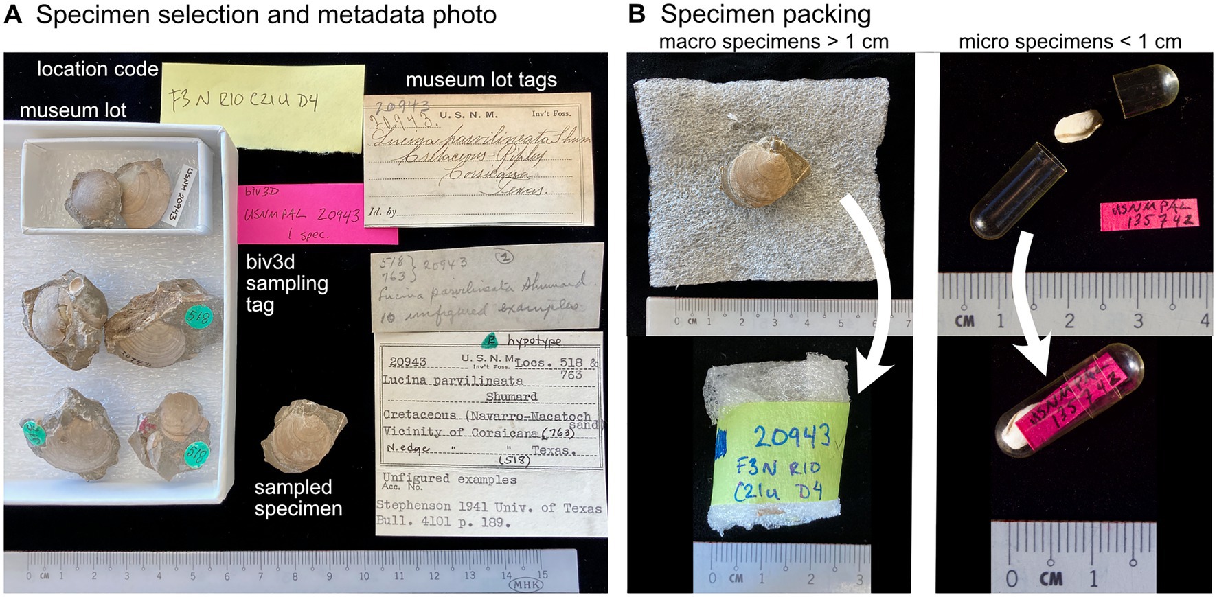
Figure 1. Workflow for sampling and packaging specimens from collections for scanning. (A) Museum lot with target specimen of Late Cretaceous fossil “Lucina” parvilineata Shumard 1861 to be imaged and temporary note marking number of specimens or valves sampled (as “biv3d sampling tag”). Location code gives the physical location of the specimen in the museum, here: Floor 3 North, Row 10, Case 21 upper, Drawer 4. (B) Macro specimens (>1 cm) are wrapped in pliable foam and secured with painter’s tape, noting the registration number and the specimen’s physical location code in the museum. Micro specimens (<1 cm) are placed in gel caps with a tag containing registration number and the specimen’s physical location in the museum (on the back of tag in this image).
At a minimum, we find that databasing the information in Table 1 is crucial to maintaining unique object identifiers and their associated metadata. It is important to record verbatim copies of the ID, locality and stratigraphy info as provided on the museum labels in order to maintain connections back to the museum database, even if those pieces of information are updated for analyses (see “lot photo” in Figure 1A). Each specimen picked for scanning receives a specimen ID (Table 1). In the case of specimens where both valves are to be scanned, a specimen ID refers to both valves, as they are part of the same specimen. This is necessary so that the two digital mesh objects representing those valves can continue to be associated in analyses by their specimen ID (each unique valve is then referenced by a mesh ID, Table 1).
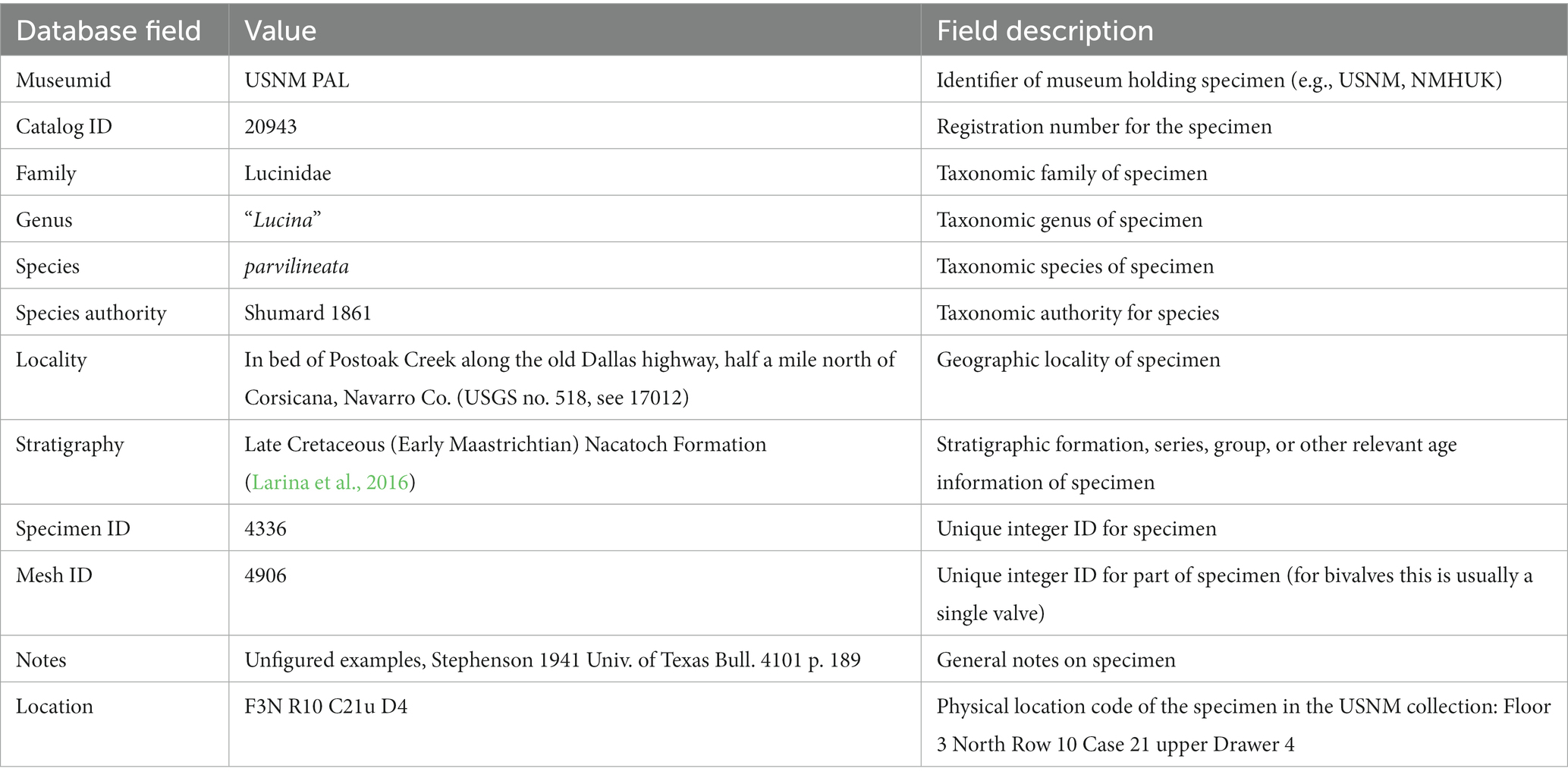
Table 1. Database schema for recording specimen information.
For all scans, the size of the smallest feature of interest determines how specimens are grouped for bulk scanning. In bivalves, a key taxonomic character—the hinge teeth—are often an order of magnitude smaller than the shell, which sets an upper limit on how many specimens may fit into the field of view of the detector. For example, on the GE Phoenix v|tome|x M 240/180 kV Dual Tube μCT with a DXR250 (16″, 4 M pixel) X-ray detector at the U.S. National Museum of Natural History (NMNH, also USNM), specimens with approximately 1 mm (1,000 μm) features of interest are sufficiently resolved using <20 μm resolution, which would characterize such features with 50 pixels in the image plane. This resolution translates to a 40 mm by 40 mm field of view on a detector 2000 × 2000 pixel detector, which can typically accommodate 4–5 approximately 10–20 mm specimens in a cylindrical arrangement. Larger specimens have larger sizes of their smallest features of interest and can be packed to similar numbers for scanning at lower resolutions; however, most bivalves have scanned best at resolutions finer than 50 μm. Fossil specimens embedded in sedimentary matrix are often scanned alone because multiple fossil specimens, particularly those in dense siliciclastics, can require higher voltage to penetrate the full object; this may exceed the power limits of the micro-CT, and it will likely reduce the contrast between the edges of the specimens and matrix, making segmentation more difficult or virtually impossible (advances in laboratory phase contrast CT could improve segmentation of materials with subtle differences in signal, see Birnbacher et al., 2021). Additionally, scanning fossils embedded in matrix at the highest possible resolution reduces artifacts such as partial volume effects, which arise as the averaging of gray values from materials with different densities in a single voxel (described further in Abel et al., 2012; Racicot, 2016).
Once specimens have been grouped for scanning, they can be mounted into cylindrical containers. Straight-sided, thin-walled plastic soda bottles with a flat, level foam insert supporting specimens from the bottom work best for holding specimens (Figure 2A). For macro specimens (>1 cm), arrange in an imbricated fashion with the shell commissure perpendicular to the base of the container (Figure 2A, i.e., mounting with the long-axis perpendicular to the X-ray source as in Sutton et al., 2014, p. 53); this arrangement reduces Feldkamp artifacts and provides the sharpest boundaries between surfaces. Specimens can be mounted in vertical layers up to a height equaling the diameter of the container (i.e., a square field of view), and packed with additional foam to prevent movement during scanning. For micro specimens (<1 cm), use paper or plastic drinking straws to hold gel caps; straws can then be inserted into 50 ml or 15 ml conical centrifuge tubes (Figure 2B), making sure to keep specimens level with each other.
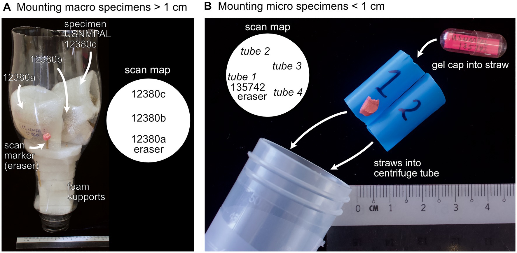
Figure 2. Mount of specimens for micro-CT imaging. (A) Macro specimens (>1 cm) are placed inside a cylindrical plastic container in an imbricated manner, with commissures perpendicular to the foam support at the base of the container. The scan map records the position of specimens in the scan mount using registration numbers or unique specimen IDs relative to the scan marker (e.g., an eraser). (B) Micro specimens (<1 cm) are placed inside plastic or paper straws, which are then placed inside a 15 ml or 50 ml centrifuge tube.
To orient the scan, place a marker into the scanning container with lower X-ray density than the specimens, such as an eraser; using markers that are more X-ray dense can shade specimens, which makes them more difficult to segment in post-processing. Draw a plan view “scan map” of the specimens relative to the marker, identifying positions using the unique identification code labeled on the specimen wrap or gel cap (Figure 2). Each scanning “cartridge” can be prepared before scanning, which is a crucial step for maximizing machine time.
Once specimens are mounted in the micro-CT, several parameters should be tuned to optimize the X-ray imaging. Each scan can, and often does, have different parameter settings, which vary according to the material density of the specimens and the number of specimens in the scan scene—or, for fossils, by the volume and mineralogy of the surrounding matrix. Because specific scanning parameters will vary by micro-CT system, we emphasize that the tuning process outlined below is intended to be generalizable; nevertheless, the parameters reported here are likely good starting points (for a comprehensive overview of optimizing scanning parameters, see Sutton et al., 2014, pp. 56–60). For all steps that follow, monitor the histogram of gray values in the imaging software; this is the crucial tool for maximizing contrast between materials in the scan.
Because we aim for high throughput, we first set parameters that affect the length of the scan to their lowest values: i.e., set exposure timing to lowest value, frame averaging to 1, and frame skips to 0. Next, we rotate the mounted specimens until viewed through the thickest portion of the scan scene; this will correspond to the lowest intensity gray values in the live image. We increase or decrease the voltage until the minimum gray value intensity recommended for the machine is reached (this ranges between 100 and 200 for the micro-CT at NMNH, trending towards the higher end as the filament ages). We aim for the lowest energy X-rays necessary to penetrate the specimen, which maximizes the contrast between materials (Sutton et al., 2014, pp. 56–57). Next, we adjust the current to maximize the total range, contrast ratio, and signal to noise of the histogram (Table 2). Increasing the current also increases the power, and tends to increase the minimum gray value, which can reduce both the signal to noise and contrast ratios (compare values in Table 2); if so, step back to previous settings. If the minimum gray cannot be reached within the power limits of the X-ray tube or without oversaturating the detector, add a physical filter (see next section) or increase the exposure timing, which may require adding frame skips so that the detector panel can discharge between images (this timing can be highly system-dependent). Similarly, it is important to check that the X-ray spot size is not 1.3 times larger than the expected voxel size (i.e., resolution) of the scan. Increasing exposure time and frame averaging will also increase the signal to noise ratio, helping to define sharper boundaries between shell and matrix if needed (often a good setting to adjust when the shell is a calcareous matrix).
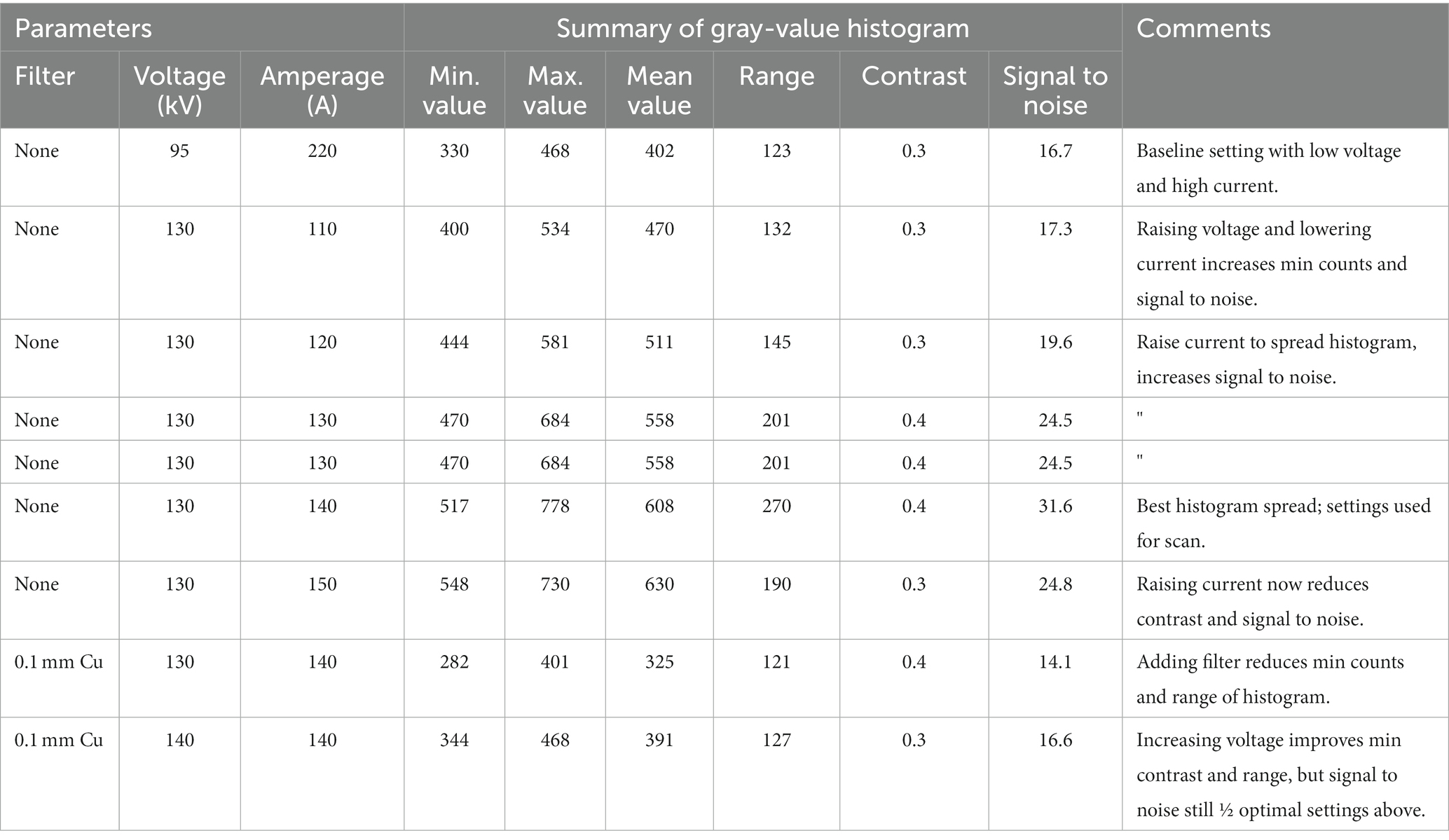
Table 2. Effects of X-ray parameter settings on gray-value histogram for scanning specimen USNM PAL 20943, “Lucina” parvilineata.
Filters can reduce beam hardening, an artifact where soft X-rays are absorbed at the sample surface leaving only the higher energy X-rays to penetrate the sample; this creates streak or cupping artifacts, where gray values grade from high to low intensity towards the interior of the specimen (see Sutton et al., 2014; Wellenberg et al., 2018). Fossil shells in matrix frequently show cupping artifacts, which can complicate simple segmentation on gray value intensity. Metal filters, typically aluminum, copper, or tin sheets ranging from 0.1 to 1 mm in thickness, can minimize this gradient in gray value intensities, but at the cost of diminished compositional contrast. Because many of our fossil shells are in calcareous matrix, meaning there is minimal compositional contrast between specimen and rock, we generally do not use filters in order to maximize what little contrast may exist. For Recent specimens free of matrix, a 0.1 mm copper filter does reduce beam hardening, simplifying segmentation of shell material from air and foam, but segmentation of scans lacking a filter is not any more difficult.
All of our scans use 360° rotation, and while the rule of thumb for setting the number of projections images is the width of the scan in pixels multiplied by π (Keklikoglou et al., 2019, p. 17), we find that shells with simple, large morphologies (i.e., smooth shells with large hinge teeth) can be scanned with projections equaling the greatest width of the scan scene (for a detector 2000 pixels wide, this would be 2000 projections). This can reduce scan times to as low as 7–10 min, depending also on the exposure time, frame averaging and skips. Thus, it is important to group specimens for bulk scanning according to the desired resolution for their smallest features of interest. For shells with relatively finer details, or for those embedded in matrix, setting a higher number of projections can better resolve those features (Sutton et al., 2014, p. 58; Keklikoglou et al., 2019, p. 7), although we find N*1.5 to usually be sufficient.
We have reconstructed all scans using the proprietary software of the micro-CT systems (i.e., GE phoenix datos|x), but alternative solutions are available (Sutton et al., 2014, pp. 149–150). We have always scanned with settings to compensate for any drift in the center of rotation, changes in focal spot size, and any small movement of the specimens (in the GE system, this would be using the Autoscan Optimizer followed by the Automatic Geometry Calibration before reconstruction). Scanning using detector shifts (i.e., small adjustments in the detector panel to reduce hot pixels), can reduce beam hardening (for additional mitigation techniques, see Wellenberg et al., 2018). Streaks, ring artifacts, and beam hardening are often in our scans and could be further mitigated during the reconstruction step—but we find these artifacts to rarely impact the final surface mesh for Recent and fossil material that is free of matrix. For fossils in matrix, application of deep learning segmentation below can help to overcome these artifacts.
Once reconstructed, Recent and fossil material that is free of matrix can often be isolated from air and packing materials by simply thresholding out the non-target values in the image stack (see a recent list of commercial software and freeware for this operation in Keklikoglou et al., 2019, their Table 15, but also see 3D Slicer Kikinis et al., 2014; we primarily use ORS Dragonfly; Object Research Systems (ORS) Inc., 2022). If the organic content of shells varies within a bulk scan (i.e., nacre vs. calcite), the scan scene may require separate threshold values for generating shell-specific regions of interest (ROIs). These shell ROIs can be further refined using manual segmentation tools, or by removing any pixels isolated from the targeted shells with simple region of interest tools, such as island processing algorithms that remove pixel sets less than a certain value (e.g., “Processing Islands” in ORS Dragonfly). From these refined ROIs, contour meshes can be generated and exported for further cleaning and morphological analysis. For many fossil shells embedded in matrix, particularly those in calcareous matrix, this simple thresholding approach will not work given the limited compositional contrast between the specimen and sediment. Here, deep learning can facilitate segmentation.
Deep learning has become a powerful tool for image segmentation, especially for digital excavation of fossils embedded in matrix (Liu and Song, 2020; Yu et al., 2022). However, we note that to date, our applications of deep learning have yet to perfectly segment a bivalve fossil from matrix (as Yu et al., 2022 also noted for segmenting dinosaur bones from matrix). Thus, we use deep learning as a technique to speed up segmentation, which almost always requires manual tuning to complete; this means finding a compromise between the time spent fitting the model(s) and then manually finalizing the segmentation. We use the deep learning interface developed by ORS Dragonfly (the “Segmentation Wizard,” Badran et al., 2020), which creates an interactive session for fitting and refining multiple deep learning models for segmentation. Regardless of the software used, we suggest that this approach is a good, generalizable workflow. Continued research into model architectures will undoubtedly bring faster and more accurate initial segmentations of these low compositional contrast materials, but our emphasis here is on producing sizable datasets of workable 3D models for quantitative evolutionary analysis. Thus, the trade-off in time spent tuning hyperparameters and fitting models in search of a perfect segmentation should be weighed against using an adequate model to provide a strong starting point for manual segmentation.
Within the ORS Dragonfly Segmentation Wizard, we begin segmentation by selecting a slice from the image stack that best represents the full diversity of features; often this is an image slice containing hinge teeth or fine ornamentation (e.g., Figure 3A). We then define the segmentation frame (i.e., a rectangular mask) that brackets the shell and manually set ROIs corresponding to shell material and background (i.e., matrix and/or air, Figure 3A, bottom row). We then train a series of deep learning models using this single frame and visually inspect the predicted segmentation (Figure 3B). Usually, the U-Net architecture (Ronneberger et al., 2015) is the fastest and most accurate approach, but Sensor3D, and variations on the U-Net such as Attention U-Net and U-Net++ can sometimes better separate the boundaries between fossil shell and matrix (hyperparameters for the U-Net fit here are in Figure 3C). The resulting model accuracies provide a general estimate of segmentation performance, but high accuracies can sometimes characterize models with poor definition of the boundary between fossil shell and matrix (e.g., frame 1 in Figure 3B for Round 1 of training, which had an accuracy score of 0.97 Figure 3D). In this example, the model trained for one round cleanly separates shell from air, but confuses parts of the matrix and shell (compare Figures 3A,B for frame 1, particularly around the hinge area). Therefore, the additional training data was labeled, and the model weights updated through continued training.
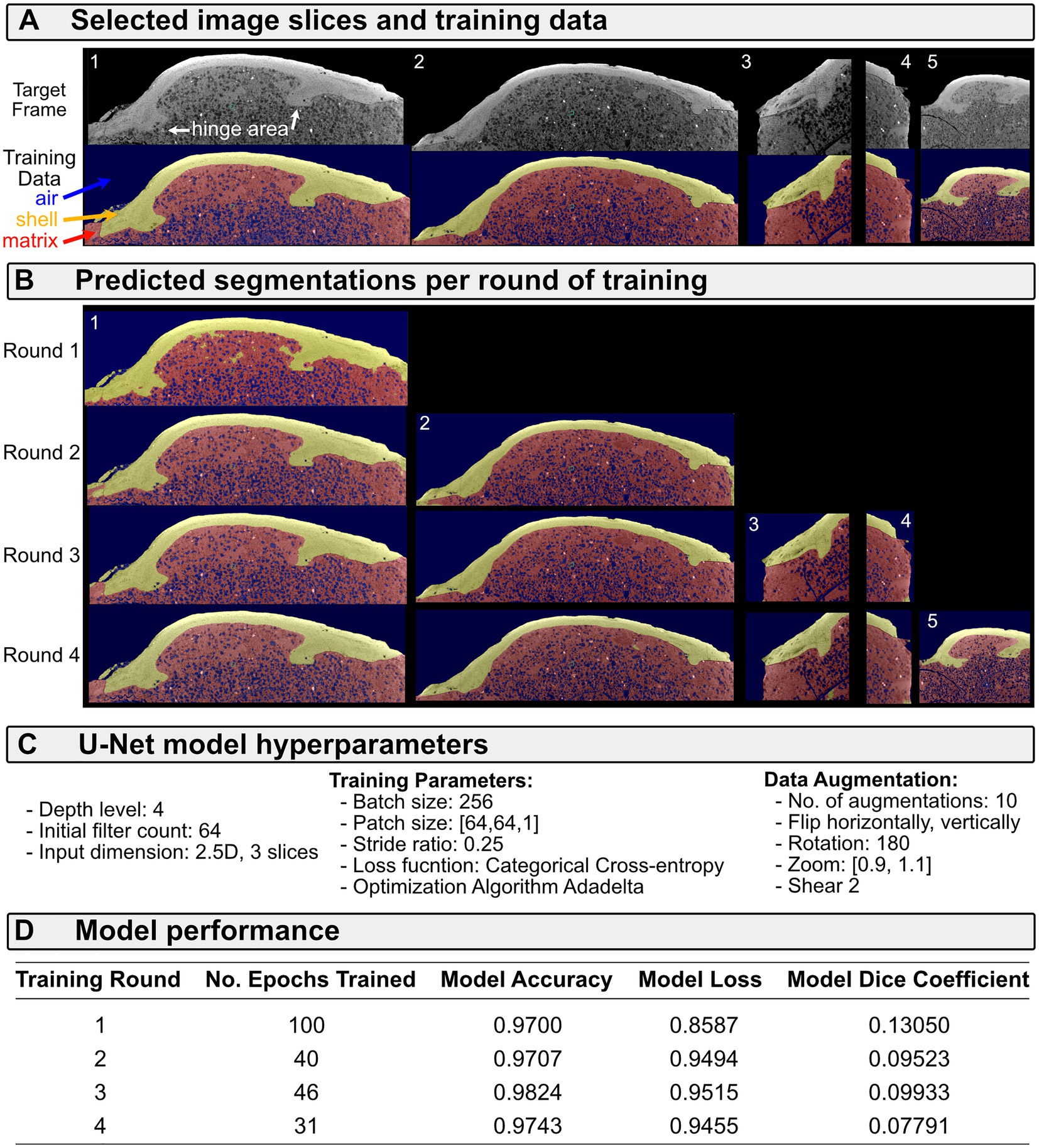
Figure 3. Segmentation of shell from matrix using deep learning for specimen USNM PAL 20943, “Lucina” parvilineata. (A) Selected image slices cropped to training frames in the top row, with frame number in white text. Bottom row shows ground-truth labeled training data. (B) Predicted segmentation for image slices per round of model training, i.e., only frame 1 was trained in round 1, but frames 1 and 2 were used to train round 2, so both have predicted segmentations for this round. Both frames 3 and 4 were included in round 3 of training. Frame 5 was only included in round 4. (C) Hyperparameters of the U-Net model. (D) Model performance statistics for each round of training.
Subsequent rounds of training improved the segmentation of shell from matrix (compare better capture of the hinge area in rounds 2–4, Figure 3B). The training data in frames 3 and 4 were selected to improve segmentation of shell from matrix where streak artifacts impacted the shell boundary at the edge of the specimen. Frame 5 was selected to improve segmentation of shell from matrix for a region of the hinge area that was not well predicted through the third training round. We could continue to iterate the process at this point, expanding the training set to include image slices with poor predicted segmentation. However, as mentioned above, we weigh the continued time in fine-tuning these segmentation models against manually tuning the segmentation. In general, we find that one or two rounds of creating training data and fitting models is sufficient to produce a strong starting segmentation. From there, we manually segment regions where the model failed to define the boundary between shell and matrix. Without any manual segmentation, the resulting 3D model has noise, but captures nearly all of the relevant taxonomic details (Figure 4). Timing required for segmentation via deep learning compared to fully manual operation depends, in part, on compute power. The process described for the fossil in Figure 3 required approximately 3 h, from labeling training data to fitting the model and predicting the segmentation, and half of that time was fitting the initial model (compute power: Intel Xeon Silver 4214R CPU @2.40 GHz with 512 GB RAM and 2 × 16 GB NVIDIA Quadro RTX5000 GPU). Fully manual segmentation of this fossil is estimated to take 8 or more hours of constantly engaged work.
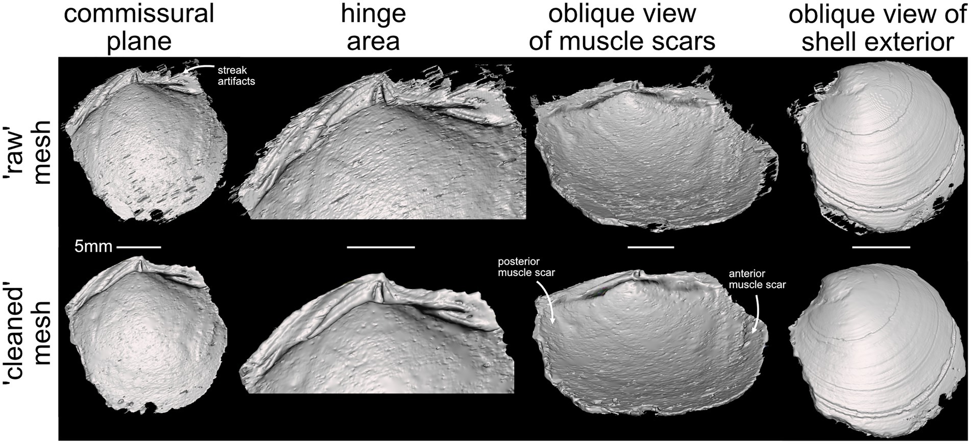
Figure 4. Taxonomically important views of the previously inaccessible interior features of Late Cretaceous (Early Maastrichtian) “Lucina” parvilineata, USNM PAL 20943. Top row shows the ‘raw’ mesh surface directly produced by deep learning segmentation after round 4 of training in Figure 3. Bottom row shows the final mesh surface after removal of streak artifacts and manual cleaning of noisy surface data where the model struggled to segment the shell from its surrounding matrix. Considerable care should be taken at this step so as not to erode any genuine, biological features.
Bivalves have been a good model system for testing macroecological and macroevolutionary theories. Aspects of their shell morphologies largely align with molecular phylogenies (Jablonski and Finarelli, 2009; Bieler et al., 2014), allowing morphologically derived phylogenetic analyses of their biogeographic, functional, and morphological evolution through deep time. Three-dimensional micro-CT scans of bivalve shells provide access to previously unseen morphologies and to measurements of morphological dimensions that have been difficult to quantify at large sample sizes. These new data are helping to address long-standing questions about evolutionary processes within the group, which we example in the following sections. Such approaches add broader phylogenetic context for general tests of ecological and evolutionary processes acting across other model systems such as fishes and birds.
Quantitative analyses of how mass extinctions reorganize the dimensions of biodiversity require rigorous phylogenetic, ecologic, and morphologic hypotheses, and micro-CT will strengthen paleontological efforts on each of these fronts. The bivalve genus Legumen was lost in the end-Cretaceous mass extinction around 66 Ma, and its phylogenetic placement and thus the impact of its loss on the subsequent morphological and ecological evolution of its higher clade was uncertain (Collins et al., 2020). This genus is known almost entirely from its external shell shape (as in Figure 5), which is notoriously homoplastic across bivalves (Stanley, 1970; Oliver and Holmes, 2006). Using micro-CT and deep learning segmentation, we were able to segment key fossil specimens from sedimentary matrix, revealing their taxonomically important hinge morphology (Collins et al., 2020). Comparing these digital excavations to the rare specimens with physical preparations of their hinge teeth confirmed the phylogenetic placement of Legumen within the most diverse bivalve family, Veneridae. Further, 3D morphometrics of its shell shape showed Legumen to be atypical for the family, occupying a distinct region of morphospace and ecospace—one that was never regained by the family during its Cenozoic diversification, instead being invaded, and perhaps preempted, by other family-level clades (Figure 5; Collins et al., 2020). Thus, the loss of Legumen becomes an important data point in larger analyses of how developmental biases and priority effects from competing clades may interact to shape the re-diversification of biodiversity following mass extinctions.
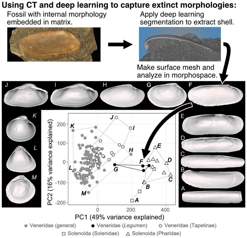
Figure 5. Using CT data to capture and analyze extinct morphologies. Fossils embedded in sediment, such as the Legumen ellipticum Conrad 1858 photographed here, can be micro-CT scanned and segmented from matrix using the deep learning approach from Figure 3. This analysis showed that the venerid genus Legumen (F, G), which was lost at the end-Cretaceous mass extinction, had an atypical shape that has yet to evolve again within the family (adapted from Collins et al., 2020).
Trade-offs in organismal form can reflect interactions of developmental constraint with ecological and environmental selection. The bivalve shell is a good vehicle for analyzing the relative impact of these factors on the sequence of evolutionary events, and their tempo and mode. For example, the volume of the bivalve’s shell compared to its soft-internal anatomy may reflect energetic trade-offs (Collins et al., 2019) and/or may proxy shell strength (Stanley, 1970), but these measurements have required molding the shell and its interior cavity (the space holding the internal soft anatomy; see Stanley, 1970, p. 109). Measuring such volumes from micro-CT-derived 3D models is now computationally simple, where volumes of triangular surface meshes can be approximated by integrating the signed tetrahedral volumes of each triangular face to the centroid of the mesh (Collins et al., 2019). Applying this approach in the comparison of a warm- to cool-temperate fauna has challenged the macroecological hypothesis that lower nutrient availability and decreased aragonite saturation states at high latitudes should filter and/or reduce the volume of the animal that is shell; both large and relatively thick-shelled bivalves are found from the Florida Keys to the Gulf of Maine (Figure 6; Collins et al., 2019). This same high-throughput approach could be used to generate high-precision estimates of intraspecific variation in relative shell volumes for taxa with known responses to gradients in ocean acidification (e.g., bimineralic Mytilus species, Bullard et al., 2021).
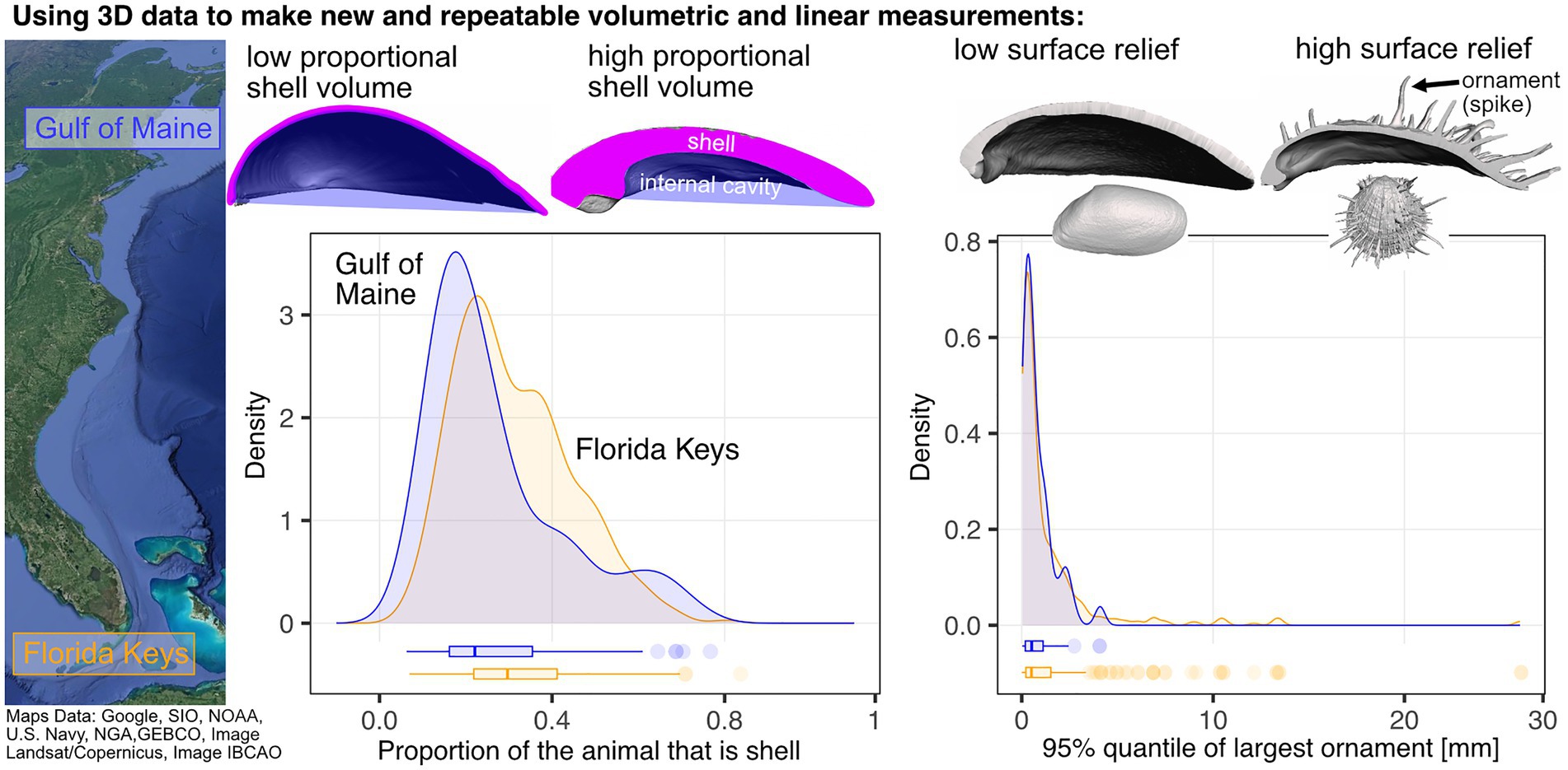
Figure 6. Using 3D data to identify latitudinal gradients in shell morphology along the east coast of North America. The proportion of the animal that is shell remains similar between the subtropical Florida Keys and temperate Gulf of Maine, but taxa with the most pronounced ornamentation do not reach the Gulf of Maine (adapted from Collins et al., 2019).
Predation intensity is another factor hypothesized to be a strong determinant of the latitudinal diversity gradient (Vermeij, 1987; Schemske et al., 2009; Freestone et al., 2021). Predation’s impact on diversity may operate on longer timescales than can be observed in real-time, and phylogenetically controlled comparative approaches are needed to augment field-based experiments. Some morphological aspects of prey have evidently evolved in direct response to modes and intensities of predation (Vermeij, 1987), and the evolution and variation of bivalve shell spines, ribs, flanges, and other elements of ornamentation are hypothesized to be anti-predatory adaptations (Vermeij, 1987; Harper and Skelton, 1993). Volumetric scans of shells have allowed us to quantify these features and analyze a significant decline in the complexity, or spininess, of shell surfaces among species from low to high latitudes, a shift that occurred by sorting among taxonomic families rather than by evolutionary transformation of genera or species (Figure 6; Collins et al., 2019). While this pattern is consistent with highest predation intensity in the tropics, it primes the investigation of other, potentially underlying factors, such as using fossils to analyze temporal lags in the biogeographic dispersion of species towards higher latitudes, and more generally to analyze regional changes in morphology that might be expected to accompany long-term climate shifts.
Since the origin of the class more than half a billion years ago, bivalves have evolved in and out of broad swaths of ecological and morphological space, offering many comparative experiments of convergence and divergence. Most analyses of morphological evolution have used 2D morphometrics of the shell, focusing primarily on its outline within the commissural plane (sagittal plane). The commissural profile captures some of the relationship between shell shape and ecological function but misses a key axis of shape variation within the transverse plane—its curvature or inflation. This morphological axis also relates to the shell’s interaction with the substratum, from the hydrodynamics of swimming in scallops to the infaunal clam’s penetration of substrata, that is, the animal’s ability to burrow away from predators and buffer open-water environmental conditions. Analyses of 3D shell shape using surface semi-landmarking capture considerable variation in shell inflation (Collins et al., 2019, p. 9; Edie et al., 2022b, p. 4), which should be taken into account when identifying instances of convergence and divergence. For example, bivalves that bore into rocks—an ecological function that can require excavating substrata that is materially harder than the shell—show a remarkable disparity of shell forms within the usually measured commissural plane, suggesting multiple, divergent evolutionary pathways into the niche. In theory, this function might drive convergence along the “hidden” third axis of variation, shell inflation, but tests including this dimension indicate this is not the case, and that rock-boring is indeed one of the most morphologically disparate functions across the class today (Collins et al., 2023).
Access to phylogenetically and morphologically broad characterizations of shell shape has introduced complications to shape-based morphometrics. For example, aligning specimens on point-based biological homology is complicated by Bivalvia having only one such point across the entire class, the origin of shell growth at the beak (Carter et al., 2012, p. 21; Edie et al., 2022a). Thus, shape-based comparative morphometrics requires alignment using a biomechanical axis that reflects how the animals interact with their environment. The hinge line—the line about which the two valves rotate during the opening and closing of the valves—is functionally analogous across the class, and can be defined using clade-specific features (Edie et al., 2022a). While not strictly adhering to the conventions of geometric morphometrics, this approach gives intuitive gradients and clusters in shell morphology that can be combined with other means of aligning shells to test hypotheses of how tightly coupled form and function are to modes of shell growth (Edie et al., 2022a).
3D morphometrics of shell shape can also address morphological integration and modularity in bivalves, with their simple skeletons that grow by accretion, and how they might contrast with clades exhibiting more complex segmented skeletons (e.g., arthropods and vertebrates). The features of the bivalve shell and the enclosed soft parts might fall into discrete functional or developmental units (Figure 7), e.g., the hinge teeth possibly showing tight covariation with the relative sizes and positions of the muscles and the spring-like ligament that together form the functional complex that opens and closes the shell. Alternatively, the shell may form a discrete, integrated module from the soft-internal anatomy. At least for the most speciose group in today’s ocean, the Veneridae, the latter appears to be true (Figure 7; Edie et al., 2022b). Thus, unlike the many modules in segmented invertebrates, the vertebrate skeleton, or even in vertebrate crania, bivalves appear to have tighter integration of their major morphological elements and a lower overall modularity (Sherratt et al., 2017; Edie et al., 2022b). Broader comparisons with other major bivalve groups could reveal a more varied pattern of modularity, integration and disparity, particularly those groups that break bilateral symmetry in shell growth and shape (Jablonski, 2020).
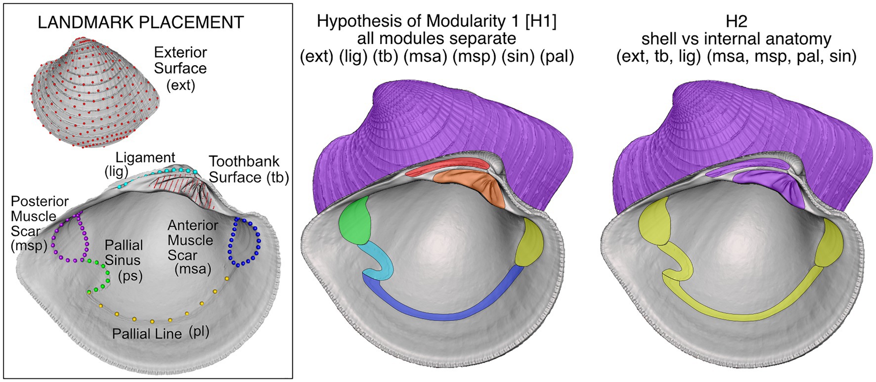
Figure 7. Geometric morphometric landmarking of shell features and hypotheses of modularity and integration in the venerid bivalve Chionopsis amathusia (Philippi 1844). Hypothesis of modularity “H1” was the working hypothesis, with all potential modules varying independently, but H2, with just two discrete modules, was best supported by morphometric analysis (adapted from Edie et al., 2022a,b).
The paleontologist’s remit in evolutionary biology has grown substantially since the Modern Synthesis (Gould, 2002; Sepkoski, 2015; Marshall, 2017; Jablonski, 2017a,b). Direct access to evolutionary sequences of morphologies is critical for understanding how innovations and other factors drive diversifications along phylogenetic, functional, and morphological lines, and how the extinction or pruning of forms impacted the trajectories of diversification. Analyses of extant-only data can sometimes proxy the former, particularly for shallow-time radiations, but they cannot address or even approximate the latter. Both patterns of morphological gain and loss are needed for robust considerations of how determinism and contingency affect evolutionary trajectories. Still, accessing this library of time-stratified morphologies remains difficult. Discovery of new fossil diversity was once limited by the scale and number of field campaigns, then by “reburial” in under-cataloged and under-digitized museums, and always by physical access to collections. Extensive efforts have steadily grown deep-time biodiversity databases, but many fossils remain locked away in consolidated sediments—in the field and in collections—making them difficult to access without painstaking collection and preparation. X-ray computed tomography overcomes some of these limitations, mobilizing virtual data and spurring substantial discovery and description of new fossils, mostly vertebrates. However, most of life today and in the past belongs to invertebrate phyla, many of which have an abundance of fossilized hard parts. Scanning and digitally excavating these fossils has been a challenge given the compositional similarity between their hard parts and the surrounding sediments, but advances in segmentation using deep learning is speeding up this process. Now, for the first time, we have views into rarely or never seen shell morphologies, such as the previously inaccessible, taxonomically important interior morphology of the “Lucina” parvilineata segmented here, laying the foundation for more complete phylogenetic consideration. Bivalves, and other invertebrates with strong fossil records including snails, echinoderms, brachiopods, trilobites, sponges, corals, and many more, are ripe for new phylogenetic and morphological evolutionary analyses facilitated by X-ray micro-CT.
The original contributions presented in the study are included in the article. Mesh of USNM PAL 20943 available on Morphosource (ark:/87602/m4/497818). Further inquiries can be directed to the corresponding author.
All authors listed have made a substantial, direct, and intellectual contribution to the work, and approved it for publication.
The study was supported by National Science Foundation EAR-1633535, DEB 2049627, National Aeronautics and Space Administration EXOB08-0089, and a CDAC Data Science Discovery grant, University of Chicago.
We thank the many museums and their staff for access to collections in their care: R. Bieler, J. Gerber, and J. Jones (Field Museum); M. Florence, E. E. Strong, and C. Walters (National Museum of Natural History); R. Portell and J. Slapcinski (University of Florida Museum of Natural History); E. A. Glover, A. Salvador, J. D. Taylor, and T. White (Natural History Museum, London); V. Delvanaz, D. Geiger, P. Valentich-Scott (SBMNH); E. Kools and P. Roopnarine (CAS). For scanning access, we thank A. I. Neander (University of Chicago Paleo-CT micro-CT facility); J. J. Hill and S. Whitaker (NMNH Scientific Imaging Facility). For discussions, we thank F. Goetz and S. Keogh. We thank E. Clark and three reviewers for constructive feedback.
The authors declare that the research was conducted in the absence of any commercial or financial relationships that could be construed as a potential conflict of interest.
All claims expressed in this article are solely those of the authors and do not necessarily represent those of their affiliated organizations, or those of the publisher, the editors and the reviewers. Any product that may be evaluated in this article, or claim that may be made by its manufacturer, is not guaranteed or endorsed by the publisher.
Abel, R., Laurini, C., and Richter, M. (2012). A palaeobiologist’s guide to “virtual” micro-CT preparation. Palaeontol. Electron. 15:15.2.6T. doi: 10.26879/284
Badran, A., Marshall, D., Legault, Z., Makovetsky, R., Provencher, B., Piché, N., et al. (2020). Automated segmentation of computed tomography images of fiber-reinforced composites by deep learning. J. Mater. Sci. 55, 16273–16289. doi: 10.1007/s10853-020-05148-7
Bauer, J. E., and Rahman, I. A. (2021). Virtual Paleontology: Tomographic Techniques for Studying Fossil Echinoderms (Elements of Paleontology). Cambridge, UK: Cambridge University Press.
Bieler, R., Mikkelsen, P. M., Collins, T. M., Glover, E. A., González, V. L., Graf, D. L., et al. (2014). Investigating the bivalve tree of life–an exemplar-based approach combining molecular and novel morphological characters. Invertebr. Syst. 28, 32–115. doi: 10.1071/IS13010
Birnbacher, L., Braig, E.-M., Pfeiffer, D., Pfeiffer, F., and Herzen, J. (2021). Quantitative X-ray phase contrast computed tomography with grating interferometry. Eur. J. Nucl. Med. Mol. Imaging 48, 4171–4188. doi: 10.1007/s00259-021-05259-6
Borowiec, M. L., Dikow, R. B., Frandsen, P. B., McKeeken, A., Valentini, G., and White, A. E. (2022). Deep learning as a tool for ecology and evolution. Methods Ecol. Evol. 13, 1640–1660. doi: 10.1111/2041-210X.13901
Bullard, E. M., Torres, I., Ren, T., Graeve, O. A., and Roy, K. (2021). Shell mineralogy of a foundational marine species, Mytilus californianus, over half a century in a changing ocean. Proc. Natl. Acad. Sci. 118:e2004769118. doi: 10.1073/pnas.2004769118
Carter, J. G., Harries, P. J., Malchus, N., Sartori, A. F., Anderson, L. C., Bieler, R., et al. (2012). Illustrated glossary of the Bivalvia. Treatise Online Vol 1. (No. 48, Part N), 1–209. doi: 10.17161/to.v0i0.4322
Claussen, A. L., Munnecke, A., Wilson, M. A., and Oswald, I. (2019). The oldest deep-boring bivalves? Evidence from the Silurian of Gotland (Sweden). Facies 65:26. doi: 10.1007/s10347-019-0570-7
Coates, M. I., Tietjen, K., Olsen, A. M., and Finarelli, J. A. (2019). High-performance suction feeding in an early elasmobranch. Sci. Adv. 5:eaax2742. doi: 10.1126/sciadv.aax2742
Collins, K. S., Crampton, J. S., Neil, H. L., Smith, E. G. C., Gazley, M. F., and Hannah, M. (2016). Anchors and snorkels: heterochrony, development and form in functionally constrained fossil crassatellid bivalves. Paleobiology 42, 305–316. doi: 10.1017/pab.2015.48
Collins, K. S., Edie, S. M., Gao, T., Bieler, R., and Jablonski, D. (2019). Spatial filters of function and phylogeny determine morphological disparity with latitude. PLoS One 14:e0221490. doi: 10.1371/journal.pone.0221490
Collins, K. S., Edie, S. M., and Jablonski, D. (2020). Hinge and ecomorphology of Legumen Conrad, 1858 (Bivalvia, Veneridae), and the contraction of venerid morphospace following the end-Cretaceous extinction. J. Paleontol. 94, 489–497. doi: 10.1017/jpa.2019.100
Collins, K. S., Edie, S. M., and Jablonski, D. (2023). Convergence and contingency in the evolution of a specialized mode of life: multiple origins and high disparity of rock-boring bivalves. Proc. R. Soc. B Biol. Sci. 290:20221907. doi: 10.1098/rspb.2022.1907
Collins, K. S., Klapaukh, R., Crampton, J. S., Gazley, M. F., Schipper, C. I., Maksimenko, A., et al. (2021). Going round the twist—an empirical analysis of shell coiling in helicospiral gastropods. Paleobiology 47, 648–665. doi: 10.1017/pab.2021.8
Cunningham, J. A., Rahman, I. A., Lautenschlager, S., Rayfield, E. J., and Donoghue, P. C. J. (2014). A virtual world of paleontology. Trends Ecol. Evol. 29, 347–357. doi: 10.1016/j.tree.2014.04.004
Daley, G., and Bush, A. (2020). The effects of lithification on fossil assemblage biodiversity and composition: an experimental test. Palaeontol. Electron. 23:a53. doi: 10.26879/1119
Edie, S. M., Collins, K. S., and Jablonski, D. (2022a). Specimen alignment with limited point-based homology: 3D morphometrics of disparate bivalve shells (Mollusca: Bivalvia). PeerJ 10:e13617. doi: 10.7717/peerj.13617
Edie, S. M., Khouja, S. C., Collins, K. S., Crouch, N. M. A., and Jablonski, D. (2022b). Evolutionary modularity, integration and disparity in an accretionary skeleton: analysis of venerid Bivalvia. Proc. R. Soc. B Biol. Sci. 289:20211199. doi: 10.1098/rspb.2021.1199
Edie, S. M., Smits, P. D., and Jablonski, D. (2017). Probabilistic models of species discovery and biodiversity comparisons. Proc. Natl. Acad. Sci. 114, 3666–3671. doi: 10.1073/pnas.1616355114
Feldmann, R., Chapman, R. E., and Hannibal, J. T. (1989). Paleotechniques. Paleontol. Soc. Spec. Publ. 4, f1–f5. doi: 10.1017/S2475262200005360
Foote, M. (1997). The evolution of morphological diversity. Annu. Rev. Ecol. Syst. 28, 129–152. doi: 10.1146/annurev.ecolsys.28.1.129
Foote, M., Crampton, J. S., Beu, A. G., and Nelson, C. S. (2015). Aragonite bias, and lack of bias, in the fossil record: lithological, environmental, and ecological controls. Paleobiology 41, 245–265. doi: 10.1017/pab.2014.16
Freestone, A. L., Torchin, M. E., Jurgens, L. J., Bonfim, M., López, D. P., Repetto, M. F., et al. (2021). Stronger predation intensity and impact on prey communities in the tropics. Ecology 102:e03428. doi: 10.1002/ecy.3428
Goswami, A., Noirault, E., Coombs, E. J., Clavel, J., Fabre, A.-C., Halliday, T. J. D., et al. (2022). Attenuated evolution of mammals through the Cenozoic. Science 378, 377–383. doi: 10.1126/science.abm7525
Gould, S. J. (2002). The Structure of Evolutionary Theory. Cambridge, MA: Belknap Press of Harvard University Press.
Harper, E., and Skelton, P. (1993). The Mesozoic marine revolution and epifaunal bivalves. Scr. Geol. 2, 127–153.
Huang, Z., Liu, Z., He, P., Ren, Y., Li, S., Lei, Y., et al. (2022). Segmentation-guided denoising network for low-dose CT imaging. Comput. Methods Prog. Biomed. 227:107199. doi: 10.1016/j.cmpb.2022.107199
Jablonski, D. (2005). Mass extinctions and macroevolution. Paleobiology 31, 192–210. doi: 10.1666/0094-8373(2005)031[0192:MEAM]2.0.CO;2
Jablonski, D. (2017a). Approaches to macroevolution: 1. General concepts and origin of variation. Evol. Biol. 44, 427–450. doi: 10.1007/s11692-017-9420-0
Jablonski, D. (2017b). Approaches to macroevolution: 2. Sorting of variation, some overarching issues, and general conclusions. Evol. Biol. 44, 451–475. doi: 10.1007/s11692-017-9434-7
Jablonski, D. (2020). Developmental bias, macroevolution, and the fossil record. Evol. Dev. 22, 103–125. doi: 10.1111/ede.12313
Jablonski, D., Belanger, C. L., Berke, S. K., Huang, S., Krug, A. Z., Roy, K., et al. (2013). Out of the tropics, but how? Fossils, bridge species, and thermal ranges in the dynamics of the marine latitudinal diversity gradient. Proc. Natl. Acad. Sci. 110, 10487–10494. doi: 10.1073/pnas.1308997110
Jablonski, D., and Finarelli, J. A. (2009). Congruence of morphologically-defined genera with molecular phylogenies. Proc. Natl. Acad. Sci. U. S. A. 106, 8262–8266. doi: 10.1073/pnas.0902973106
Johnston, P., and Haggart, J. (Eds.) (1998). Bivalves: An Eon of Evolution. Calgary: University of Calgary Press.
Keklikoglou, K., Faulwetter, S., Chatzinikolaou, E., Wils, P., Brecko, J., Kvaček, J., et al. (2019). Micro-computed tomography for natural history specimens: a handbook of best practice protocols. Eur. J. Taxon 522, 1–55. doi: 10.5852/ejt.2019.522
Kikinis, R., Pieper, S. D., and Vosburgh, K. G. (2014). “3d slicer: a platform for subject-specific image analysis, visualization, and clinical support” in Intraoperative Imaging and Image-Guided Therapy. ed. F. A. Jolesz (New York, NY: Springer), 277–289.
Larina, E., Garb, M., Landman, N., Dastas, N., Thibault, N., Edwards, L., et al. (2016). Upper Maastrichtian ammonite biostratigraphy of the Gulf coastal plain (Mississippi embayment, southern USA). Cretac. Res. 60, 128–151. doi: 10.1016/j.cretres.2015.11.010
Leshno Afriat, Y., Edelman-Furstenberg, Y., Rabinovich, R., Todd, J. A., and May, H. (2021). Taxonomic identification using virtual palaeontology and geometric morphometrics: a case study of Jurassic nerineoidean gastropods. Palaeontology 64, 249–261. doi: 10.1111/pala.12521
Liu, X., and Song, H. (2020). Automatic identification of fossils and abiotic grains during carbonate microfacies analysis using deep convolutional neural networks. Sediment. Geol. 410:105790. doi: 10.1016/j.sedgeo.2020.105790
Marshall, C. R. (2017). Five palaeobiological laws needed to understand the evolution of the living biota. Nat. Ecol. Evol. 1:0165. doi: 10.1038/s41559-017-0165
Matsukuma, A. (1996). Transposed hinges: a polymorphism of bivalve shells. J. Molluscan Stud. 62, 415–431. doi: 10.1093/mollus/62.4.415
Object Research Systems (ORS) Inc. (2022). Dragonfly 2022.2 [Computer Software]. Available at: http://www.theobjects.com/dragonfly (Accessed December, 2022).
Oliver, P. G., and Holmes, A. M. (2006). The Arcoidea (Mollusca: Bivalvia): a review of the current phenetic-based systematics. Zool. J. Linnean Soc. 148, 237–251. doi: 10.1111/j.1096-3642.2006.00256.x
Prôa, M., Pouit, D., Rouillard, T., Vincent, P., and Mellier, B. (2021). Hidden treasures uncovered: successful detection of fossils below the surface in large limestone blocks using a standard medical X-ray CT scanner. Foss. Impr. 77, 36–42. doi: 10.37520/fi.2021.004
Racicot, R. (2016). Fossil secrets revealed: X-ray CT scanning and applications in paleontology. Paleontol. Soc. Pap. 22, 21–38. doi: 10.1017/scs.2017.6
Reid, M., Bordy, E. M., Taylor, W. L., le Roux, S. G., and du Plessis, A. (2019). A micro X-ray computed tomography dataset of fossil echinoderms in an ancient obrution bed: a robust method for taphonomic and palaeoecologic analyses. GigaScience 8:giy156. doi: 10.1093/gigascience/giy156
Ronneberger, O., Fischer, P., and Brox, T. (2015). “U-Net: convolutional networks for biomedical image segmentation” in Medical Image Computing and Computer-Assisted Intervention – MICCAI 2015 lecture notes in computer science. eds. N. Navab, J. Hornegger, W. M. Wells, and A. F. Frangi (Cham: Springer International Publishing), 234–241.
Schemske, D. W., Mittelbach, G. G., Cornell, H. V., Sobel, J. M., and Roy, K. (2009). Is there a latitudinal gradient in the importance of biotic interactions? Annu. Rev. Ecol. Evol. Syst. 40, 245–269. doi: 10.1146/annurev.ecolsys.39.110707.173430
Schwarzhans, W., Beckett, H. T., Schein, J. D., and Friedman, M. (2018). Computed tomography scanning as a tool for linking the skeletal and otolith-based fossil records of teleost fishes. Palaeontology 61, 511–541. doi: 10.1111/pala.12349
Sepkoski, D. (2015). Rereading the Fossil Record: The Growth of Paleobiology as an Evolutionary Discipline. Chicago, IL: University of Chicago Press.
Serb, J. M., Alejandrino, A., Otárola-Castillo, E., and Adams, D. C. (2011). Morphological convergence of shell shape in distantly related scallop species (Mollusca: Pectinidae). Zool. J. Linnean Soc. 163, 571–584. doi: 10.1111/j.1096-3642.2011.00707.x
Serb, J. M., Sherratt, E., Alejandrino, A., and Adams, D. C. (2017). Phylogenetic convergence and multiple shell shape optima for gliding scallops (Bivalvia: Pectinidae). J. Evol. Biol. 30, 1736–1747. doi: 10.1111/jeb.13137
Sherratt, E., Serb, J. M., and Adams, D. C. (2017). Rates of morphological evolution, asymmetry and morphological integration of shell shape in scallops. BMC Evol. Biol. 17:248. doi: 10.1186/s12862-017-1098-5
Stanley, S. M. (1970). Relation of shell form to life habits of the Bivalvia (Mollusca). Geol. Soc. Am. Mem. 125, 1–282. doi: 10.1130/MEM125
Sutton, M. D., Rahman, I. A., and Garwood, R. J. (2014). Techniques for Virtual Palaeontology. Hoboken, NJ: Wiley Blackwell.
Sutton, M., Rahman, I., and Garwood, R. (2017). Virtual paleontology—an overview. Paleontol. Soc. Pap. 22, 1–20. doi: 10.1017/scs.2017.5
Thompson, J. R., Cotton, L. J., Candela, Y., Kutscher, M., Reich, M., and Bottjer, D. J. (2021). The Ordovician diversification of sea urchins: systematics of the Bothriocidaroida (Echinodermata: Echinoidea). J. Syst. Palaeontol. 19, 1395–1448. doi: 10.1080/14772019.2022.2042408
Valentine, J. W. (1973). Evolutionary Paleoecology of the Marine Biosphere. Englewood Cliffs, NJ: Prentice-Hall.
Vermeij, G. J. (1987). Evolution and Escalation: An Ecological History of Life. Princeton, NJ: Princeton University Press.
Vermeij, G. J. (2013). Molluscan marginalia: hidden morphological diversity at the bivalve shell edge. J. Molluscan Stud. 79, 283–295. doi: 10.1093/mollus/eyt036
Wellenberg, R. H. H., Hakvoort, E. T., Slump, C. H., Boomsma, M. F., Maas, M., and Streekstra, G. J. (2018). Metal artifact reduction techniques in musculoskeletal CT-imaging. Eur. J. Radiol. 107, 60–69. doi: 10.1016/j.ejrad.2018.08.010
Keywords: paleontology, bivalve, 3D morphometrics, high-throughput morphometry, deep learning, computed tomography, CT image segmentation
Citation: Edie SM, Collins KS and Jablonski D (2023) High-throughput micro-CT scanning and deep learning segmentation workflow for analyses of shelly invertebrates and their fossils: Examples from marine Bivalvia. Front. Ecol. Evol. 11:1127756. doi: 10.3389/fevo.2023.1127756
Edited by:
Elizabeth Clark, University of California, Berkeley, United StatesReviewed by:
H. David Sheets, Canisius College, United StatesCopyright © 2023 Edie, Collins and Jablonski. This is an open-access article distributed under the terms of the Creative Commons Attribution License (CC BY). The use, distribution or reproduction in other forums is permitted, provided the original author(s) and the copyright owner(s) are credited and that the original publication in this journal is cited, in accordance with accepted academic practice. No use, distribution or reproduction is permitted which does not comply with these terms.
*Correspondence: Stewart M. Edie, ZWRpZXNAc2kuZWR1
Disclaimer: All claims expressed in this article are solely those of the authors and do not necessarily represent those of their affiliated organizations, or those of the publisher, the editors and the reviewers. Any product that may be evaluated in this article or claim that may be made by its manufacturer is not guaranteed or endorsed by the publisher.
Research integrity at Frontiers
Learn more about the work of our research integrity team to safeguard the quality of each article we publish.