Enhancing landslide management with hyper-tuned machine learning and deep learning models: Predicting susceptibility and analyzing sensitivity and uncertainty

Introduction: Natural hazards such as landslides and floods have caused significant damage to properties, natural resources, and human lives. The increased anthropogenic activities in weak geological areas have led to a rise in the frequency of landslides, making landslide management an urgent task to minimize the negative impact. This study aimed to use hyper-tuned machine learning and deep learning algorithms to predict landslide susceptibility model (LSM) and provide sensitivity and uncertainty analysis in Aqabat Al-Sulbat Asir region of Saudi Arabia.

Methods: Random forest (RF) was used as the machine learning model, while deep neural network (DNN) was used as the deep learning model. The models were hyper-tuned using the grid search technique, and the best hypertuned models were used for predicting LSM. The generated models were validated using receiver operating characteristics (ROC), F1 and F2 scores, gini value, and precision and recall curve. The DNN based sensitivity and uncertainty analysis was conducted to analyze the influence and uncertainty of the parameters to the landslide.

Results: Results showed that the RF and DNN models predicted 35.1–41.32 and 15.14–16.2 km² areas as high and very high landslide susceptibility zones, respectively. The area under the curve (AUC) of ROC curve showed that the LSM by the DNN model achieved 0.96 of AUC, while the LSM by RF model achieved 0.93 of AUC. The sensitivity analysis results showed that rainfall had the highest sensitivity to the landslide, followed by Topographic Wetness Index (TWI), curvature, slope, soil texture, and lineament density.

Discussion: Road density and geology map had the highest uncertainty to the landslide prediction. This study may be helpful to the authorities and stakeholders in proposing management plans for landslides by considering potential areas for landslide and sensitive parameters.

1. Introduction

Landslides are considered the second most destructive geo-hazard that cause serious problems, such as widespread damage to property and infrastructure, loss of natural resources and, more importantly, human lives, according to the United Nations Development Program (Huang and Zhao, 2018; Azarafza et al., 2021; Tanyu et al., 2021). Each year, landslides claim several lives and cause billions of US dollars in property damage. According to a World Bank report, about 300 million people live in landslide-prone areas, and about 600 people are killed annually by landslides (World Bank, 2005). In addition, it is estimated that global landslides cause $20 billion worth of economic damage (Mezősi, 2022). On the other hand, nations like the United States of America, Italy, India, China, and Germany suffer significant losses annually (Zou and Zheng, 2022).

Furthermore, landslides are inherently very uncertain due to the complex function of various factors, such as geological complexity, topographical influences, land use and landscape changes (Loche et al., 2022; Mantovani et al., 2022). Also, the occurrence of landslides can be caused by various factors, including heavy precipitation, volcanic eruptions, seismic activities such as earthquakes, elevation and slope of a surface, vegetation cover, soil properties, and even human activities like the construction of roads, buildings, and agricultural practices (Liu and Ding, 2020; Gunturu, 2022). In this regard, the development of more accurate landslide susceptibility models (LSMs) based on accurate landslide inventories is essential (Orhan et al., 2020). Therefore, there is a need to map landslide susceptibility to identify areas that could potentially be affected by landslides.

Recently, landslide susceptibility has attracted a great deal of attention from researchers worldwide, where landslides have been a recurring problem. This could be an empirical response to this natural geo-hazard that could help those responsible for land decisions and land use planning. In general, the techniques that are utilized in the mapping of landslide susceptibility can be categorized as either qualitative or quantitative techniques (Nath et al., 2021; Sweta et al., 2022). The qualitative methods take a more subjective approach and rely on the knowledge and experience of experts to assign weights to the various factors that could have caused the effect (Roy et al., 2019). In order to get around the restrictions associated with the qualitative methods; the quantitative methods take an objective approach and are purely statistical or data-driven approach that examines the interrelationship between landslide and its controlling factors for predicting susceptibility zones (Das et al., 2022). The field of quantitative techniques has seen much focus on using remote sensing (RS) and geographical information systems (GIS) over the past few years. These methods have provided reliable and promising results for landslide prediction all over the world.

Furthermore, in recent decades, there has been widespread use of statistical models, and machine learning algorithms (MLAs), for various applications in landslide studies. MLAs such as artificial neural networks (ANN) (Benbouras, 2022), decision trees (DT) (Pham et al., 2020; Arabameri et al., 2021), support vector machines (SVM) (Daviran et al., 2022; Saha et al., 2022), random forest (RF) (Deng et al., 2022; Kavzoglu and Teke, 2022), classification and regression trees (CART) (Orhan et al., 2020; Alqadhi et al., 2021), neuro-fuzzy (Mehrabi, 2021), etc., enhance spatial results and show good landslide vulnerability performance to be used in land management. Although machine learning models for LSM are widely used, they also have certain weaknesses such as their high dependence on the training and testing data and poor predictive accuracy (Bui et al., 2020; Gautam et al., 2021; Saha et al., 2021). To overcome this issue, the hybrid models such as ensemble machine learning models and meta-heuristic algorithm have been proposed for the LSM modeling (Song et al., 2021; Alqahtani et al., 2022). Compared to standalone models, these hybrid models can quickly identify the non-linearity of input and output variables since these models are flexible and become more robust with noisy data (Ibrahim et al., 2022). However, the hybrid models are also complex methods and take a long time, and require a difficult search for a good meta-heuristic algorithm among many models with diverse architectures. In comparison to the standalone and hybrid machine learning models, the deep learning models may reduce these limitations in the LSM modeling (Prasad et al., 2022; Xi et al., 2022). In the field of artificial intelligence, Deep Learning and Deep Neural Network (DNN) have recently become the most influential approaches. In light of this, experts in the field of landslide hazard modeling have begun to investigate the effectiveness of deep learning techniques for solving this problem. Compared to more traditional shallow learning methods, deep learning typically produces different results in the feature engineering and extraction stages of the training process (Tien Bui et al., 2020; Yao et al., 2022). Standard shallow learning models, such as backpropagation neural networks, logistic regression and DT, create decision boundaries from scratch using only the initial feature set provided by the database GIS. Deep learning is a subfield of machine learning that involves the use of ANN to model complex patterns and relationships in data (Azarafza et al., 2021). Unlike traditional machine learning methods that rely on hand-crafted features, deep learning algorithms can automatically learn and extract high-level features from raw data, allowing them to achieve state-of-the-art performance in a wide range of tasks, including image and speech recognition, natural language processing, and robotics (Daviran et al., 2022; Saha et al., 2022). There are several deep learning algorithms, such as convolutional neural network (CNN), recurrent neural network (RNN), long-short term memory, which have been widely proposed and applied successfully in other areas of environmental modeling, such as climate modeling, hydrology, and ecology (Gavrishchaka et al., 2018; Tien Bui et al., 2020; Prasad et al., 2022; Xi et al., 2022; Yao et al., 2022).

However, DNNs among other deep learning models can be an effective choice when the available data is limited, as they can still perform well with a relatively small amount of data (Gavrishchaka et al., 2018; Shang et al., 2021; Yao et al., 2022). This is because DNNs can learn hierarchical representations of the input data, which can capture complex patterns and relationships even with limited data.

In comparison, other types of deep learning models such as CNNs and RNNs typically require large amounts of data to achieve good performance, especially for tasks such as image or speech recognition (Achu et al., 2021; Shang et al., 2021; Dela et al., 2022).

However, it’s important to note that DNNs also require careful hyperparameter tuning to achieve optimal performance, even in data-scarce conditions (Achu et al., 2021). Hyperparameters such as the number of hidden layers, the number of neurons in each layer, the learning rate, and the regularization strength can significantly affect the performance of the mode (Achu et al., 2021).

Tien Bui et al. (2020) used a DNN to create landslide risk assessment models and compared its performance to a hybrid machine learning model. They found that the DNN model had comparable prediction performance to the hybrid model. However, there is still a need for further research to investigate and compare the performance of DNN models for different types of applications, and to explore the potential of using different learning algorithms for training DNN models. Consequently, this paper develops the newly developed DNN model within the H₂O framework based on landslide susceptibility mapping by using gradient descent, root mean square propagation and adaptive moment optimization techniques.

However, remote sensing and other data-intensive technologies have made it possible to gather large volumes of data about the environment, which can be used to inform management decisions. However, in many cases, data scarcity remains a major challenge, particularly in developing countries and remote regions. In such situations, machine learning models can help to extract information from limited datasets and support decision-making.

Random forest is a popular MLA that has been widely used for remote sensing applications due to its ability to handle small data and provide accurate predictions. However, RF may not always perform optimally in situations where the data is limited, and it may require large datasets to produce accurate land surface models (LSMs). In contrast, DNN has shown promise in producing accurate LSMs but typically require large datasets to achieve their full potential.

One potential solution is to use DNN models in data-scarce regions by tuning the hyper-parameters of DNN and RF. This approach can help the model to learn data patterns from fewer datasets and accurately predict new data, even in regions where data scarcity is a significant issue. This approach is novel and provides a practical solution to the challenge of limited data availability in remote regions.

Another issue in management is sensitivity analysis, which involves identifying the responsible parameters that have the most significant impact on model performance. Traditional statistical models have been used to conduct sensitivity analysis. Previous studies have employed SOBOL indices based on variance, expanded FAST, Moris one at a time (OAT), and a linear regression model (Hsieh et al., 2018; Liu and Ding, 2020; Xue et al., 2021; Dela et al., 2022; Li et al., 2022). These models are also very good in determining the effect of input parameters on output parameters. However, DNN models have not yet been utilized for this purpose. The use of hyper-tuned DNN models to conduct sensitivity analysis is an innovative approach that can provide valuable insights into the key parameters that need to be considered in decision-making. Hence, the use of hyper-tuned DNN models and sensitivity analysis can help to overcome the challenge of data scarcity and provide valuable information for management decisions. These novel approaches can provide accurate LSMs, early warning systems, and other management tools that are essential for sustainable development in remote regions.

After reviewing the literature, the objective of this study is to develop a robust LSM using grid search-based hypertuned machine learning and deep learning models under H₂O open-source framework, and to analyze the sensitivity and uncertainty of parameters using DNN based sensitivity analysis in predicting LSM.

2. Materials and methods

2.1. Study area

Aqabat Al-Sulbat is located on the Abha-Bahah Road in the Asir region of Saudi Arabia and covers an areas of 199 km² (Figure 1). The elevation of the study area ranges from 989 to 2404 m. Geologically, the area belongs to the Ablah Group, which is dominated by the Farwah Shear Zone and lies between the Al Lith-Bidah and Shwas-Tayyah structural belts. The Jerub Formation, the Rafa Formation, and the Thurat Formation are examples of the three formations found within this group. These formations, together with the others, form a sequence of volcanic and epiclastic rocks. There are a large number of fractures, most of which divide the granite into cubic or quadrangular blocks. All joints are weathered and eroded. The study site is cold and semi-arid. On average, 218 mm of precipitation occur per year, with February to June accounting for 75 percent of the total. The average maximum and minimum temperatures are 29.5 and 16.8°C, respectively.

FIGURE 1

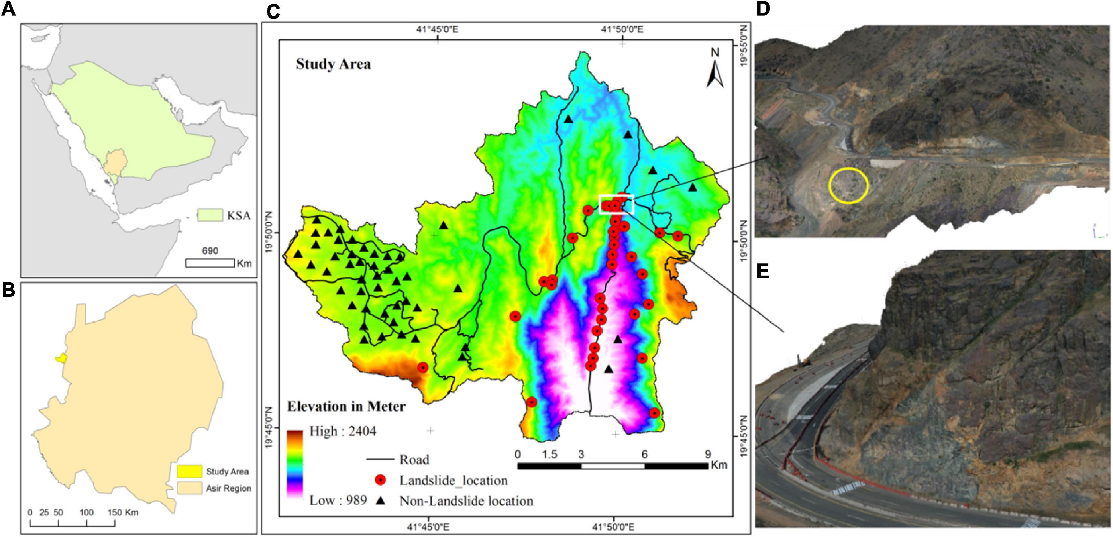
Figure 1. Showing the study area, landslide sites (A) Saudi Arabia with Asir region; (B) Asir region with the study area location; (C) the study area, landslide site and non-landslide site and (D,E) 3D model of landslide site (white circle showing landslide-prone area).

2.2. Dataset

In this work, several sources were used to acquire landslide triggering variables. NASA’s Earth Science Data Systems provided the ALOS PALSAR DEM. Sentinel-2 MSI has been downloaded from USGS Earth Explorer.¹ The 1:100,000 Saudi Geological Survey map was used to create the geological map. The field survey yielded the information on the soil’s texture. Google earth images and ArcGIS 10.5 software were used to create the drainage map and road.

2.3. Landslide inventory

Landslide inventories are needed for both training and testing the LS model. This study identified landslide areas by field surveys and official sources (Figure 1). The construction of roads and buildings in the study area has increased in muddy terrain, making it more vulnerable to landslides. Additionally, landslides are also caused by rainfall in the area. Using GPS and Google Earth, 50 landslide sites were identified in the study area, and classification-based LS modeling with binary data was used. Tang et al. (2020) suggested using a similar set of negative points or non-landslide areas, but selecting non-landslide samples can be challenging. In this study, we selected 50 locations that were not affected by landslides with the help of landslide data, local knowledge, and Google Earth. According to geotechnical experts and government papers, the areas where landslides did not occur are real and can be used for training and testing data sets. In countries where data is scarce and technology is developing, Landsat imagery, official records, and local opinions are used by researchers. We created a binary inventory dataset by assigning landslides and non-landslides 0 and 1 for classification-based LSM. The inventory data, which included 100 landslide and non-landslide polygon locations, were converted into point form (900 points). Following the approach of Saha et al. (2022), we created training and test datasets from the inventory dataset using a 70–30 ratio.

2.4. Landslide triggering variables

The susceptibility model for landslides is built on data from past events and potential triggers, as noted in reference (Saha et al., 2022). However, setting suitable input parameters can be challenging, and expert knowledge and previous literature can be used to select landslide triggers. To model susceptibility to landslides, variables such as elevation, slope, aspect, curvature, geology, soil texture, land use/cover, drainage density, lineament, distance to road, normalized difference vegetation index (NDVI), and topographic wetness index (Topographic Wetness Index) are utilized.

Elevation plays a critical role in influencing numerous factors such as vegetation, runoff direction, drainage density, landslide gravitational energy, and human activity (Nhu et al., 2020). An increase in altitude can increase the likelihood of slope failure and prolong the slope’s longevity (Pham et al., 2020). Elevation data is usually obtained from the digital elevation model (DEM), which shows elevations ranging from 2404 to 989 m in this study area (Figure 2A).

FIGURE 2

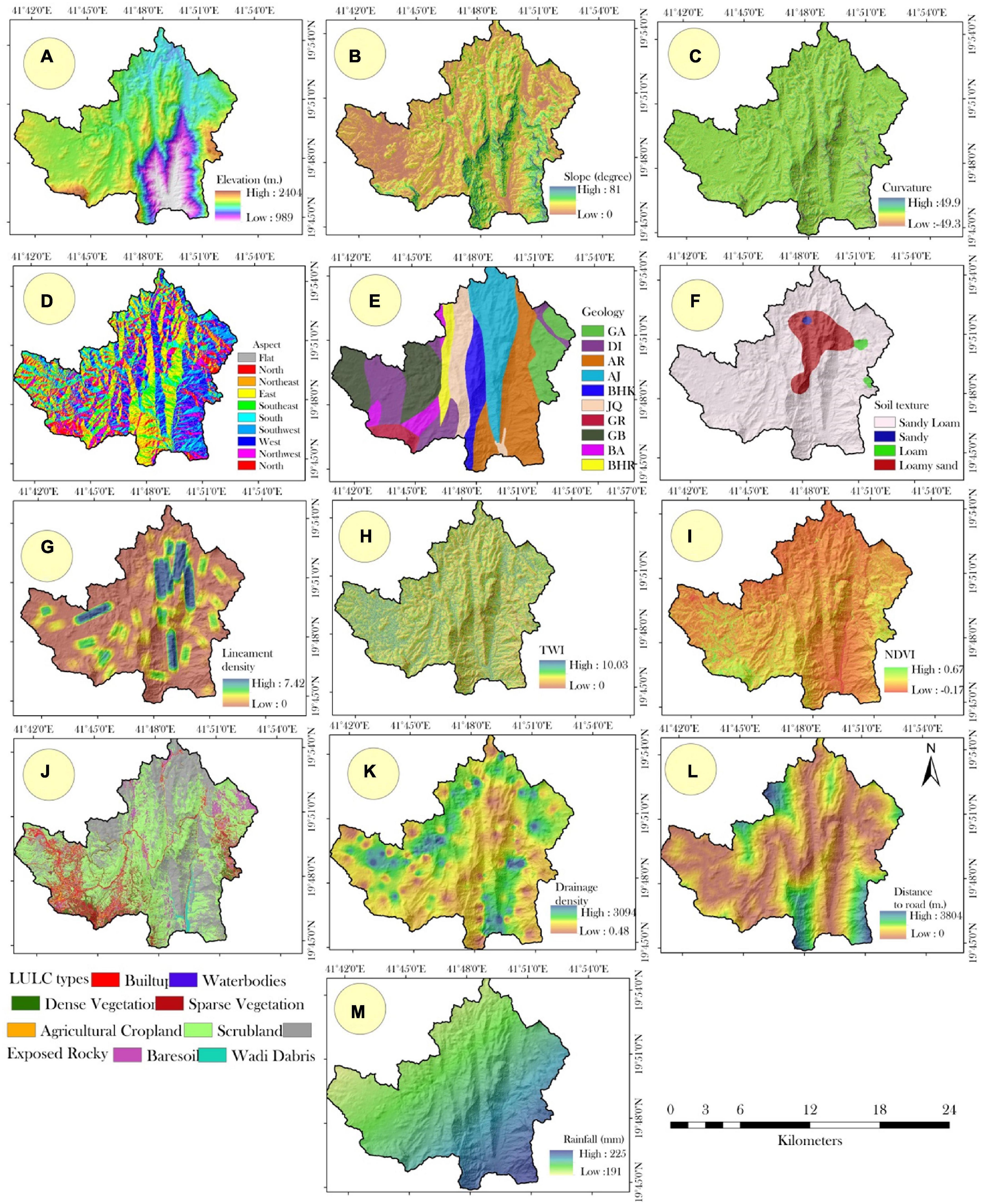
Figure 2. The landslide triggering factors, such as (A) elevation, (B) slope, (C) curvature, (D) aspect, (E) geology, (F) soil texture, (G) lineament density, (H) topographic wetness index (TWI), (I) normalized differentiation vegetation index (NDVI), (J) land use land cover (LULC) types, (K) drainage density, (L) distance to road, (M) rainfall.

Most landslides can be traced back to unstable slopes (Remondo et al., 2008; Leonardi et al., 2020), which indicates that slope is a crucial factor in regulating landslides (Lee and Min, 2001). The slope map used in this study was obtained from ALOS PALSAR DEM (Figure 2B). In addition, landslides are often associated with curved features in the landscape, and a curved surface can affect runoff and infiltration. The three possible radii of curvature, including concave (negative), flat (zero), and convex (positive curvature), have varying effects, with convex slopes producing more runoff than concave ones (Lee and Min, 2001). The terrain’s sphericity affects water drainage in mountains, as shown in Figure 2C.

Aspect refers to the slope direction, and it was derived from the DEM of the study region, which created the aspect map with categories such as flat, north, northeast, east, southeast, south, southwest, west, and northwest (Figure 3D). The physical properties of rocks, which are governed by the types and compositions of those rocks, influence the degree to which a slope is unstable or collapses. The geological map of the region, scaled at 1:100,000, was digitized by the Saudi Geological Survey, and a raster format was created using the “spatial analyst” module in ArcGIS. The study area’s geology map has ten geological classes (Figure 2E).

FIGURE 3

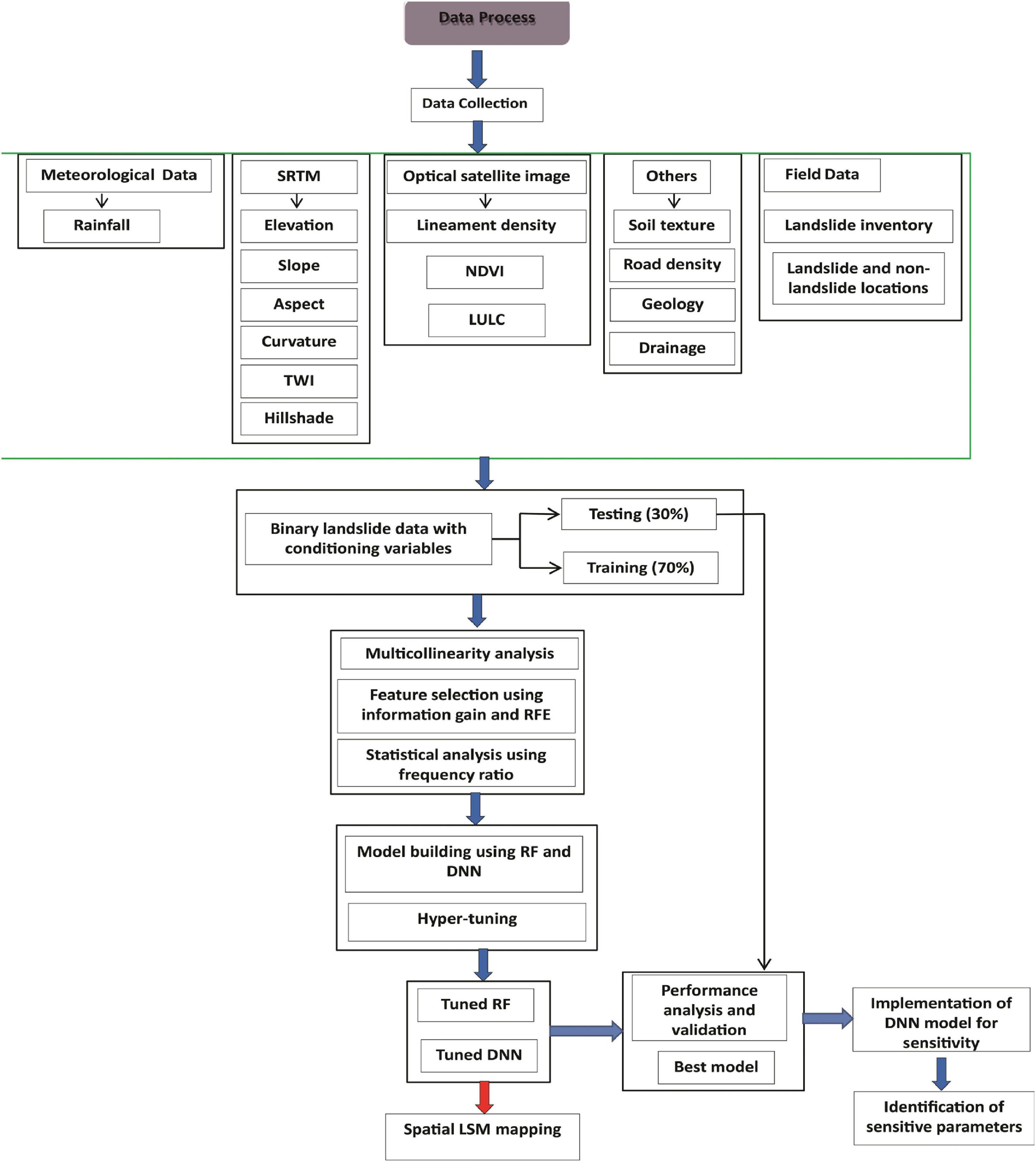
Figure 3. Methodological hierarchy for employed methods in the study area.

To analyze soil texture, 32 soil samples were taken from the study area, and the size of individual soil grains was measured using a hydrometer. The study area has different soil types, as shown in Figure 2F. Lineaments, which are long, narrow fissures in rock that weaken the material, are also crucial landslide factors, as weak geology or lineaments can increase the likelihood of landslides. Sentinel-2 satellite imagery was used in this study to extract lineaments in ENVI, and a line density tool was used to construct the resulting map of linearity density (Figure 2G).

The likelihood of landslides is influenced by increased lineament, which can be mitigated through the use of hydrologic measures provided by WI. TWI detects water accumulation in basins and helps to control slope failure and landslides caused by pore water pressure resulting from soil moisture. A high TWI is associated with increased landslides, as seen in our investigation where TWI varied from 0 to 10.03 (Figure 2H). NDVI also affects landslides by altering soil hydrology through vegetation covers that increase precipitation interception, evapotranspiration, and infiltration. Greater plant life was observed in the western part of our study area (Figure 2I), where we extracted vegetation using bands 8 and 4 of Sentinel-2 data. The presence of vegetation helps to increase the strength of soil and mitigate the threat of landslides. Land use and land cover changes can also affect slope durability, as seen in our LULC map constructed using data from Sentinel-2, where we identified built-up, water bodies, thick vegetation, sparse vegetation, agricultural farming, scrubland, exposed rocks, bare soil, and wadi debris as LULC categories in the study area (Figure 3J). We utilized MLCC classifiers for LULC mapping.

Drainage density also plays a critical role in the potential for landslides, as seen in studies where the drainage density was highest in the east (Figure 2K). We created a drain map using Google Earth and imported it into ArcGIS for drainage density analysis. Building roads on steep terrain can compromise slope stability and lead to slope failure and landslides, as cracks in the road surface created by construction and movement make materials on a slope more brittle, filling with water and causing landslides. Intense precipitation can further hasten the collapse of slopes and increase the likelihood of landslides. Mountainous regions close to roadways are especially susceptibility to landslides, as observed in our road map digitized from Google Earth, where more roads were found in the southeastern part of the study area (Figure 2L).

Rainfall is a significant factor in landslide occurrence, as it can trigger landslides by increasing pore water pressure, decreasing soil strength, and altering soil structure. The collected rainfall data from 30 rain gauges installed by Ministry of Environment, Water and Agriculture (MOEWA), Saudi Arabia in the study area, Asir region, is crucial for evaluating the rainfall-induced landslide susceptibility. The quality of rainfall data must be checked to ensure accuracy and reliability in the analysis. The annual average rainfall in the study area ranges from 225 to 191 mm, which provides essential information for determining the threshold values of rainfall intensity and duration required to trigger landslides (Figure 2M).

2.5. Method for multicollinearity analysis

Multicollinearity is a method employed in a model of logistic regression that employs closely connected independent variables. As a result, one independent variable can be predicted with a high degree of accuracy by other variables. Multicollinearity has no effect on the model’s reliability or predictability. Nonetheless, it influences the estimation power of each independent variable individually (Talukdar et al., 2021). Variance inflation factors (VIF), paired scatter plots, tolerance, and other methods can be utilized to test for multicollinearities. Multicollinearity among the variables was computed in this study using VIF and tolerance. The VIF statistic applies least squares regression (Naikoo et al., 2022) to measure multicollinearity’s strictness. In the present experiment, the VIF was employed to assess multicollinearity.

2.6. Feature selection techniques

Feature selection plays a crucial role in improving the accuracy and efficiency of machine learning models. By selecting the most relevant features, it reduces the dimensionality of the dataset, which in turn reduces the risk of overfitting and makes the model more interpretable. Feature selection also helps to identify the most important variables in the dataset, providing valuable insights for domain experts and decision makers. In this study, we used RFE and information gain ratio as feature selection techniques for evaluating the landslide conditioning parameters.

2.6.1. Recursive feature elimination (RFE)

Recursive feature elimination (RFE) is a feature selection technique that is based on the idea of recursively removing the least important features until a predetermined number of features is reached. The importance of each feature is estimated by the model coefficients, which are used to rank the features. The features with the lowest coefficients are then removed, and the process is repeated until the desired number of features is reached.

The RFE technique can be applied to various models, including linear regression, logistic regression, and SVM. It has been shown to be effective in reducing overfitting and improving model performance by selecting the most relevant features.

2.6.2. Information gain ratio

Information gain ratio is another feature selection technique that is commonly used in decision tree algorithms. It is based on the concept of entropy, which is a measure of the uncertainty of a variable. The information gain ratio measures the reduction in entropy achieved by splitting the data on a particular feature. It is calculated as the ratio of the information gain to the intrinsic information of the feature. The information gain is calculated as the difference between the entropy of the parent node and the weighted average of the entropies of the child nodes. The intrinsic information is a measure of the randomness of the feature and is calculated as the entropy of the feature. The information gain ratio is given by the following equation:

$Information\hspace{0.17em}Gain\hspace{0.17em}Ratio=$

$Information\hspace{0.17em}Gain\hspace{0.17em}/\hspace{0.17em}Intrinsic\hspace{0.17em}Information$

where the information gain is calculated as:

$InformationGain=$

$Entropy\left(parent\right)-\sum \left[weight\left(child\right)xEntropy\left(child\right)\right]$

and the intrinsic information is calculated as:

$IntrinsicInformation=-\sum \left[weight\left(child\right)xlog2\left(weight\left(child\right)\right)\right]$

where weight (child) is the fraction of the data points that belong to the child node, and Entropy (parent) and Entropy (child) are the entropies of the parent and child nodes, respectively.

The information gain ratio is used to rank the features based on their relevance to the target variable. Features with a high information gain ratio are considered to be more relevant and are therefore selected for the model.

2.7. Frequency ratio

The frequency ratio (FR) method is a statistical approach used in landslide susceptibility assessment that considers the ratio of the frequency of landslides in a given area to the frequency of landslides in the rest of the study area. This method assumes that the frequency of landslides is influenced by the distribution of causal factors, which are assumed to be spatially correlated. Therefore, this method evaluates the relative importance of these factors in controlling landslide occurrence. The FR values for each factor are calculated as the ratio of the frequency of landslides that occurred in the areas with that factor to the frequency of landslides that occurred in areas without that factor.

The FR method has been widely used in landslide susceptibility assessment due to its simplicity and efficiency in identifying the most important factors influencing landslide occurrence. The main advantage of this method is that it does not require detailed information about the spatial distribution of causal factors, which are often difficult to obtain. However, this method assumes that the factors influencing landslide occurrence are independent of each other, which is often not the case. Additionally, the method can be affected by the size and shape of the study area, which can influence the calculation of the FR values. The equation for calculating the FR value for a specific factor is:

$\begin{array}{c}FR=\left(numberoflandslideoccurrencesinareaswiththefactor\right)/\hfill \\ \left(numberoflandslideoccurrencesinareaswithoutthefactor\right)/\hfill \\ \left(totalnumberofareaswiththefactor\right)/\hfill \\ \left(totalnumberofareaswithoutthefactor\right)\hfill \end{array}$

where the numerator represents the frequency of landslides in areas with the factor, and the denominator represents the frequency of landslides in areas without the factor. The denominator is then divided by the total number of areas with and without the factor to normalize the result. The FR value for each factor is then used to rank the factors according to their relative importance in controlling landslide occurrence.

2.8. Method for landslide susceptibility mapping

2.8.1. Deep neural network (DNN)

Deep neural networks have become increasingly popular in recent years, as they offer several advantages over traditional MLAs, such as higher accuracy and the ability to handle large and non-linear datasets (Talukdar et al., 2021; Costache et al., 2022; Naikoo et al., 2022). DNNs are also able to solve complex non-linear problems and perform hierarchical feature selection. In this study, a multilayer feed-forward deep learning architecture is applied under the H₂O framework, which is similar to the conventional multi-layer perceptron (MLP).

The input parameters’ weight is computed in each neuron and passed on to the next using a transfer function. The model comprises three layers: an input layer, multiple hidden layers, and an output layer. The H₂O framework is a high-level ANN with back-propagation optimization (stochastic gradient descent) technique (Yao et al., 2022). The deep learning algorithm has been tuned using a random grid search technique with fivefold cross-validation on the training data in the H₂O framework.

The H₂O framework has several advantages, such as distributed computing, efficient memory management, and the ability to handle large datasets (Yao et al., 2022). The back-propagation optimization technique used in the H₂O framework enables the DNN to learn from the training data and improve its accuracy. The use of the random grid search technique with cross-validation helps to find the optimal hyperparameters for the DNN and prevents overfitting. The combination of these techniques provides a powerful tool for analyzing large and complex datasets, and has the potential to improve accuracy and reduce the time and resources required for analysis.

2.8.2. Random forest

Random Forest (Breiman, 2001) is a popular ensemble learning technique that combines multiple DT to make more accurate predictions. In the H₂O framework, the RF algorithm uses bootstrap aggregation (bagging) and feature sub-sampling to build an ensemble of DT.

The RF algorithm in H₂O first creates a set of DT, each one trained on a random subset of the training data and a random subset of the features. The tree is constructed by recursively splitting the data based on the feature that gives the most information gain. At each split, the algorithm selects a random subset of features to consider, reducing the likelihood of overfitting.

Once all the DT have been constructed, the algorithm aggregates their predictions to make a final prediction. In classification problems, the final prediction is usually the class that receives the most votes from the DT, while in regression problems, it is usually the average of the predicted values.

The RF algorithm in H₂O also includes a number of hyperparameters that can be tuned to improve its performance. These include the number of trees in the forest, the maximum depth of the trees, the minimum number of samples required to split an internal node, and the minimum number of samples required to be at a leaf node.

The performance of the RF algorithm can be evaluated using various metrics, such as accuracy, precision, recall, and F1 score. These metrics provide information about the ability of the algorithm to correctly classify instances in the data.

The equation for RF algorithm in H₂O is as follows:

$F\left(x\right)=1/T^{*}{\displaystyle \mathrm{\Sigma }t}=1,Tft(x)$

where F(x) is the predicted output of the ensemble, T is the number of trees in the forest, and ft(x) is the predicted output of the t-th tree. The predicted output of the ensemble is calculated as the average of the predicted outputs of all the trees in the forest.

2.9. Validation of the methods

The Receiver Operating Characteristic (ROC) curve is a graphical representation of the performance of a binary classifier system as its discrimination threshold is varied. The ROC curve plots the true positive rate (TPR) against the false positive rate (FPR) for different threshold values. TPR is also known as sensitivity or recall, and it is calculated as the ratio of the true positive to the sum of true positive and false negative. FPR is calculated as the ratio of the false positive to the sum of false positive and true negative. An ideal classifier system will have an ROC curve that passes through the upper left corner of the plot, which corresponds to a TPR of 1 and an FPR of 0.

The F1 score is the harmonic mean of the precision and recall of a binary classifier system. It provides a balance between precision and recall, and it is calculated as the ratio of the product of precision and recall to the sum of precision and recall. The F2 score is a weighted harmonic mean of the precision and recall, where the recall has more weight than the precision. The gini value is a measure of the degree of inequality in a distribution, and it is commonly used as a performance metric for DT and RFs. The equations for these metrics are as follows:

$TruePositiveRate\left(TPR\right)=$

$TruePositive/(TruePositive+FalseNegative)$

$FalsePositiveRate\left(FPR\right)=$

$FalsePositive/(FalsePositive+TrueNegative)$

$F1Score=\mathrm{\hspace{0.33em}2}{}^{*}\left(Precision{}^{*}Recall\right)/(Precision+Recall)$

$F2Score=\mathrm{\hspace{0.33em}5}{}^{*}\left(Precision{}^{*}Recall\right)/$

$(4{}^{*}Precision+Recall)GiniValue=\mathrm{\hspace{0.33em}2}{}^{*}AUC-\mathrm{\hspace{0.33em}1}$

where Precision is the ratio of true positive to the sum of true positive and false positive, Recall is the same as TPR, and AUC is the area under the ROC curve. These metrics are commonly used to evaluate the performance of classification models in various domains such as healthcare, finance, and natural language processing.

2.10. Sensitivity and uncertainty analysis

Deep neural networks, often known as DNNs, are ANN that include numerous hidden layers and an increasing number of neurons in each hidden layer. The theoretical background has been presented in methodological section [see section “2.8.1 Deep neural network (DNN)”]. These networks were developed specifically for the purpose of addressing complicated issues. DNN is more accurate than ANN, but it takes much more time and processing capacity to run.

In the present study, to best of author’s knowledge, first time we used DNN based sensitivity and uncertainty analysis for RUSEI prediction. Many previous researches have used sensitivity analysis for water quality prediction, climatic prediction, hydrologic variable prediction and other fields. They used variance based SOBOL indices, extended FAST, Moris one at time (OAT), linear regression based model (Glen and Isaacs, 2012; Jaxa-Rozen and Kwakkel, 2018; Garcia et al., 2019). Those models are also highly effective to evaluate the effect of input parameters on the output parameter. But neural network and DNN based sensitivity and uncertainty analysis has not been implemented yet in urban research.

In the present study, we implemented this model in two ways, first we implemented DNN and imported the model into sensitivity analysis framework. The theoretical background of DNN has been provided in the previous methodological section (see section 2.4.2). After obtaining the best DNN model, the weights and neural structure of the model have been extracted using the “get_weights()” of the “keras; package.” Then, we used the “SensAnalysisMLP()” function of “Neuralsens” package to perform the sensitivity and uncertainty analysis on the extracted object and same datasets, which were trained using DNN. Thus, three sensitivity measures of the output (predicted RUSEI by four models) have been computed in respect to the input parameters. The sensitivity measures are (a) input variables mean effect over the output, (b) variance of the input variable’s effect over the input, and (c) measures of input parameters in the point of view of perturbation analysis, which means larger changes in output can be experienced if small changes in the input parameters has been done. However, the meaningful information can be extracted from the relationship between mean and variance effect of input parameters over output parameters. The relationship can be as follows:

If both mean and variance of the input parameters are toward zero, which shows no relationship between input and output because the sensitivity of the output on that particular input is about zero.

If mean of the input has different value rather than zero and variance has value toward zero, it can be called linear relationship between input and output because the sensitivity of the output on that particular input is about constant. The uncertainty analysis was computed using density plot by considering mean and standard deviation of sensitive value of output, which shows the uncertainty of the output with the respect to the data distribution pattern of the input parameters. The coefficient of variation (CV) has been computed to analyze the degree of variance of the data distribution pattern for uncertainty analyze.

The whole methodological framework has been presented in Figure 3.

3. Results

3.1. Computation of multicollinearity analysis

In this study, multicollinearity among independent variables was evaluated using VIF and Tolerances (TOL). The absence of multicollinearity problem was observed as the VIF was less than 10 and tolerance was greater than 0.20 for each variable. The LSM was developed by utilizing all fourteen parameters in the current study, and it was found that the highest VIF was associated with drainage density, followed by elevation and soil texture. However, the lowest VIF was observed in aspect, geology, LULC, lineament density, and TWI. As the highest and lowest VIF for this study were far below the VIF of 10, it can be concluded that there was no multicollinearity problem among the input parameters, and all the input parameters can be utilized for the modeling process. This is an important finding for the development of accurate landslide susceptibility maps, as it indicates that all the input parameters can be included in the model without any risk of bias caused by multicollinearity. The utilization of all input parameters can contribute to the development of a comprehensive and reliable LSM.

3.2. Feature selection analysis

IGR is a measure used to evaluate the worth of an attribute in a decision tree. It calculates the amount of information gained by splitting the data based on the values of the attribute. In general, a higher IGR value indicates that the attribute is more useful in predicting the target variable. In this case, the IG.CORElearn function was used to calculate the IGR values of each variable. The result shows that the Curvature variable has the highest IGR value (0.47), followed by Rainfall (0.80), Slope (0.76), and Hillshade (0.45), which suggests that these variables are more important in predicting the target variable (Figure 4A). On the other hand, NDVI has the lowest IGR value (0.07), which indicates that this variable is less useful in predicting the target variable. Similarly, Geology, Road density, and Soil texture have relatively lower IGR values, indicating that they are less important in predicting the target variable.

FIGURE 4

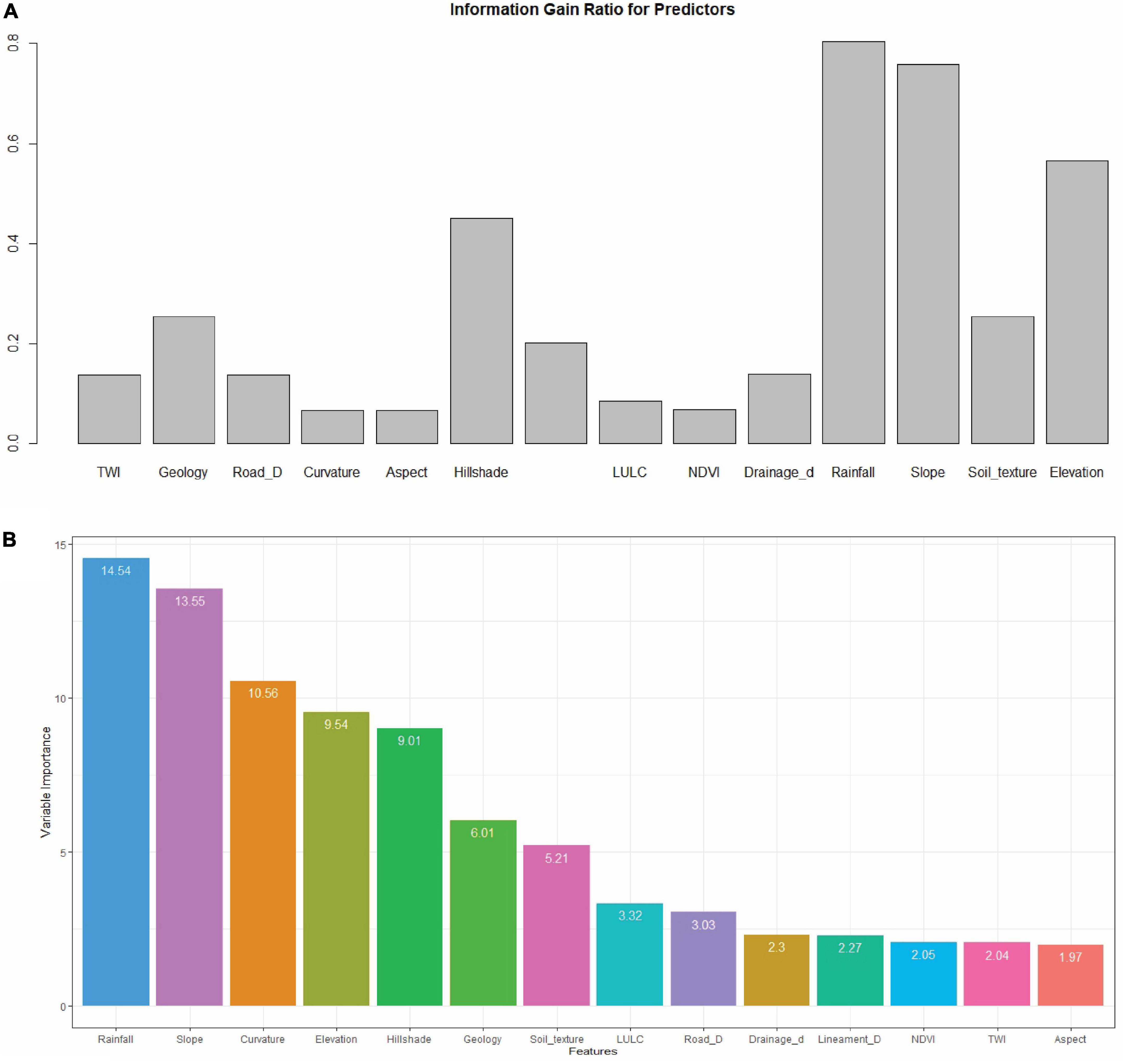
Figure 4. Feature selection for evaluating the landslide conditioning factors using (A) information gain ratio, (B) RFE.

Recursive feature elemination is a feature selection method that selects the most relevant subset of variables from a large set of variables. It is based on the idea of repeatedly training a model and removing the least important feature(s) until the optimal subset of features is found. In this specific result, RFE was performed using a cross-validated (10-fold, repeated 5 times) outer resampling method (Figure 4B). The performance of the model was measured in terms of accuracy and Kappa over subset size from 1 to 14 variables.

The results show that the accuracy and Kappa increase as the number of variables included in the model increases. The highest accuracy and Kappa are achieved when using five variables, after which the performance plateaus. The five variables that are most important for predicting the target variable are Rainfall, Slope, Curvature, Elevation, and Hillshade, according to the variable importance analysis. The variable importance analysis ranks the 14 variables based on their importance in the model (Figure 4B). Rainfall is the most important variable, followed by Slope, Curvature, Elevation, and Hillshade. The remaining variables have relatively lower importance.

3.3. Statistical analysis of parameters

The FR is a commonly used measure to identify the importance of individual variables in classification problems, particularly in landslide susceptibility studies. FR is a ratio of the proportion of events (e.g., landslides) in a certain category or range of a variable to the proportion of non-events (e.g., non-landslides) in the same category or range.

In this case, the FR values have been computed for 14 variables, including continuous variables (TWI, road density, curvature, aspect, hillshade, NDVI, drainage density, rainfall, lineament density and elevation) and categorical variables (Geology, LULC, Soil texture). The FR values range from 0.73 to 3.18, with higher values indicating that the corresponding variable is more important in distinguishing landslides from non-landslides (Figure 5). From the results provided, we can see that the parameters with the highest FR values are curvature (2.762), slope (3.184), and TWI (0.733), indicating a positive association with landslide occurrence. Parameters with an FR value close to 1, such as NDVI (0.996) and Elevation (0.830), are weakly associated with landslide occurrence. Other parameters such as rainfall (1.056), lineament density (1.395), and LULC (1.281) have moderate association with landslide occurrence. Geology (0.866), hillshade (0.704), and soil texture (1.250) have weaker associations with landslide occurrence compared to other parameters.

FIGURE 5

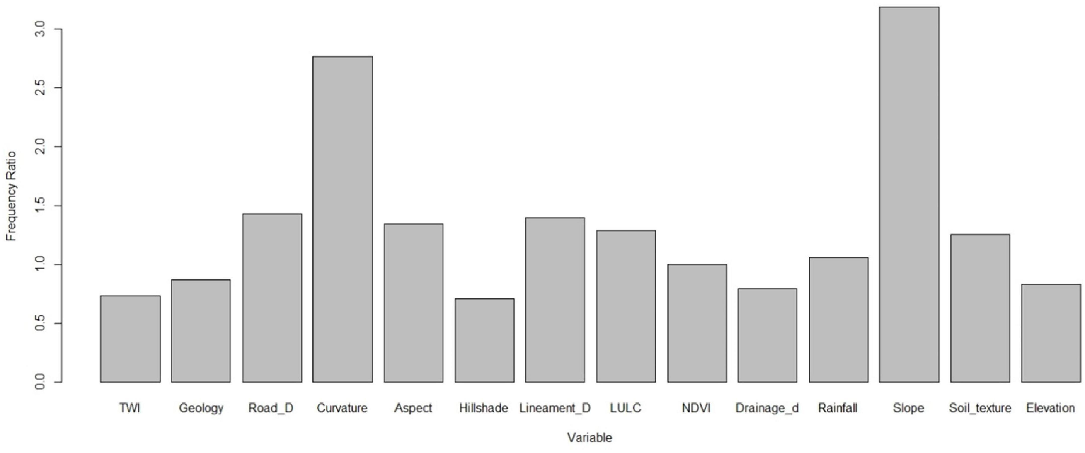
Figure 5. The variable importance for triggering landslide using frequency ratio.

For example, curvature has the highest FR value of 2.76, indicating that it is an important variable in distinguishing landslides from non-landslides. This is not surprising, as curvature is often used as a proxy for slope instability and has been shown to be a useful predictor of landslides. Similarly, slope has a relatively high FR value of 3.18, indicating that it is also an important variable in landslide susceptibility. On the other hand, variables such as NDVI and elevation have relatively low FR values (less than 1), indicating that they may be less important in distinguishing between landslides and non-landslides.

It is important to note that FR is a simple measure that does not take into account the interactions between variables or the potential for multicollinearity. Therefore, it is often used in conjunction with other measures, such as correlation analysis, to better understand the relationships between variables and their importance in predicting landslides.

3.4. Implementation of hypertuned machine learning and deep learning algorithms

In this research, we aimed to achieve the robust and highly accurate landslide susceptibility map using RF and DNN models. Many previous researches have utilized default RF and DNN model and produce LSM. But the issue is that the model that has been employed for prediction needed to be perfectly set, otherwise the default model or not-set model cannot produce highly accurate LSM. The RF and DNN models have several components that should be optimized or set by trial and error process. But the trial and process can take many times to find the optimal parameters for the models. Therefore, in this study, we first decided to find the best values for several components. For DNN models, we aimed to find the best value for activation function, numbers of hidden layers, epochs, regularization (l1 and l2), rate, rate annealing, rho, epsilon, momentum start, momentum stable, and max w2. For the RF models, we optimized the following components, ntrees, mtry, max depth, min rows, nbins, and sample rate. We provided very low to very high value to these component, applied grid search techniques. We set the model to produce top 100 models for DNN and unlimited for RF model as per the accuracy of training and testing data. Then, we arrange all the models based on the value of misclassification. Thus, we obtained 100 models for DNN and 132 models for RF algorithms to predict LSM. Figures 6, 7 show that the computation of importance variable for predicting LSM using all DNN and RF models. Figure 6 shows that all DNN models computed that NDVI and rainfall are most important parameters for LSM, while geology and curvature have less importance in predicting LSM. In addition, Figure 4 shows that rainfall, slope, NDVI, and drainage density are most important for LSM as per all RF models, while aspect, TWI, and curvature are less important parameters. Therefore, both models have difference results for finding the most important parameters for LSM; therefore, to find this, further research is required.

FIGURE 6

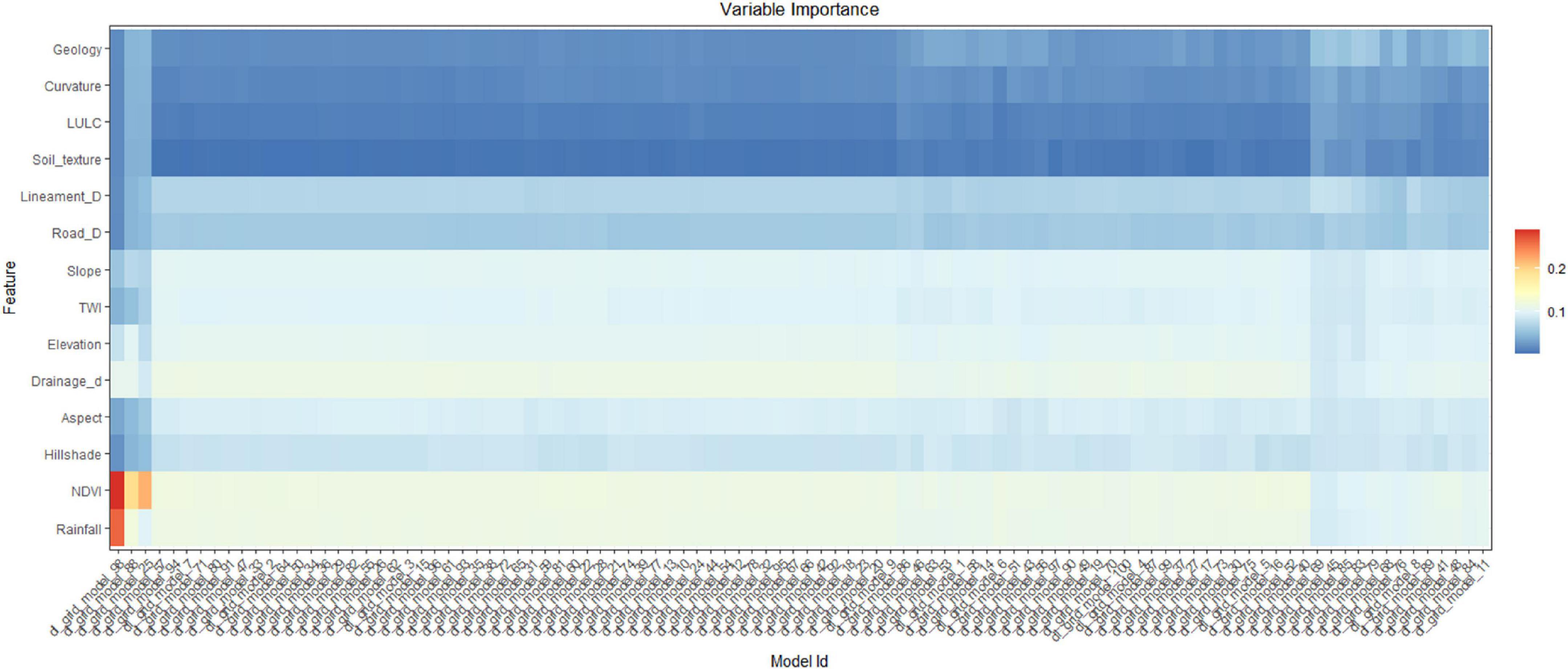
Figure 6. Computation of important variables for predicting LSM as per the top 100 DNN models.

FIGURE 7

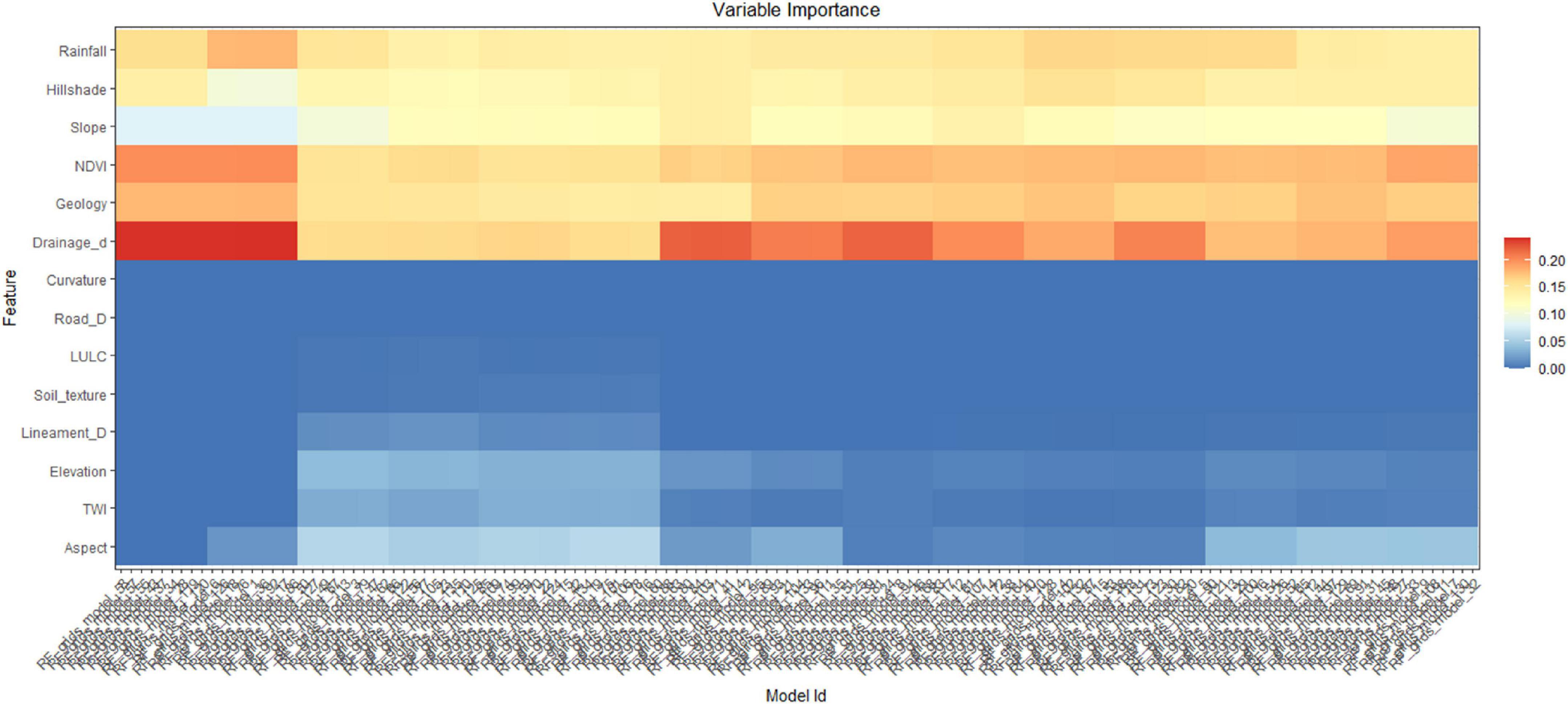
Figure 7. Computation of important variables for predicting LSM as per the top 132 RF models.

After arranging as DNN and RF models in ascending order based misclassification rate, the model with lowest error rate has been considered as best model. In this study, 20th and 10th models of DNN and RF have been considered as best model, which have very less error. These models have been used for LSM prediction in the study area. However, before proceeding for implementing the model at raster datasets, it is necessary to diagnosis whether the model is well-fit or not. Therefore, the learning curves for best DNN and RF models have been plotted in Figure 8. It is usually used to diagnosis the underfit, overfit, and well-fit model. The learning curve has been plotted with log-loss rate (error metric) against epochs (learning progress) for training, testing, and cross validation sets. Figure 8A shows that error for training loss has been stabled at 110 epochs, while the validation loss has also been stabled at the same epoch. The difference of error between training and validation loss has a close gap. Therefore, it can be considered that the best DNN model is well-fit model. In addition, the learning curve for best RF model shows very close gap between training and validation loss (Figure 8B). It is almost 0.1. Therefore, this model can also be stated as well-fit model.

FIGURE 8

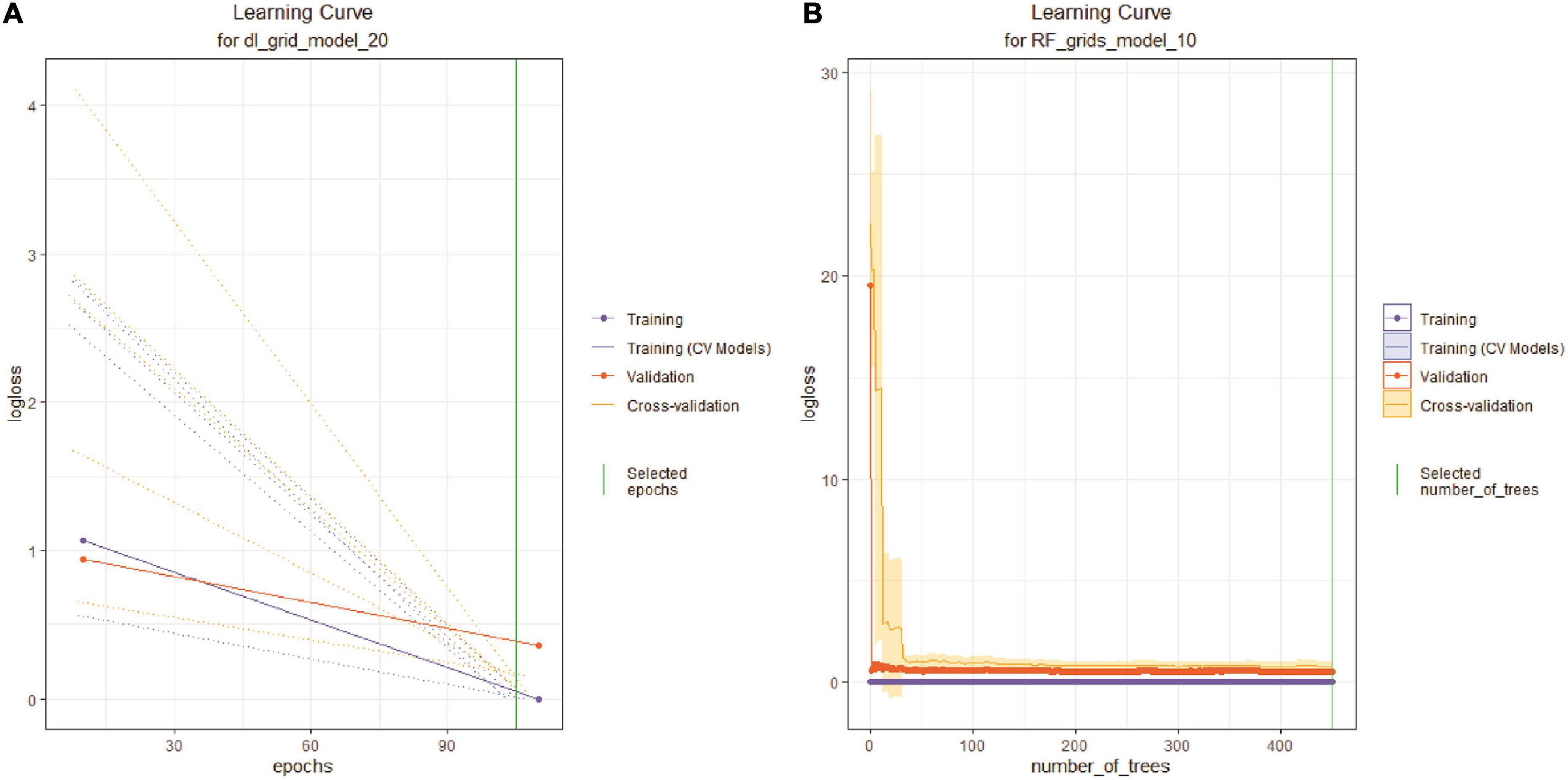
Figure 8. Learning curve for diagnosing the fitness of the model for (A) DNN, and (B) RF models.

The graphical representation of the gain and lift chart has been employed for DNN and RF models based on testing data to see how the predict models capture the response (LSM) by targeting the certain amount of sample. This chart shows the performance of the selected model on the new data (testing data). It shows that 98% of the data can be captured by DNN model by targeting only 50% of the sample. This indicates high quality performance by the DNN mode for predicting LSM based on testing dataset (Figure 9A). In addition, for RF model, 85% of the data can be captured by targeting only 50% of the sample data. Therefore, it also indicates higher performance for predicting new data (Figure 9B). But the performance of DNN model is very high than RF model.

FIGURE 9

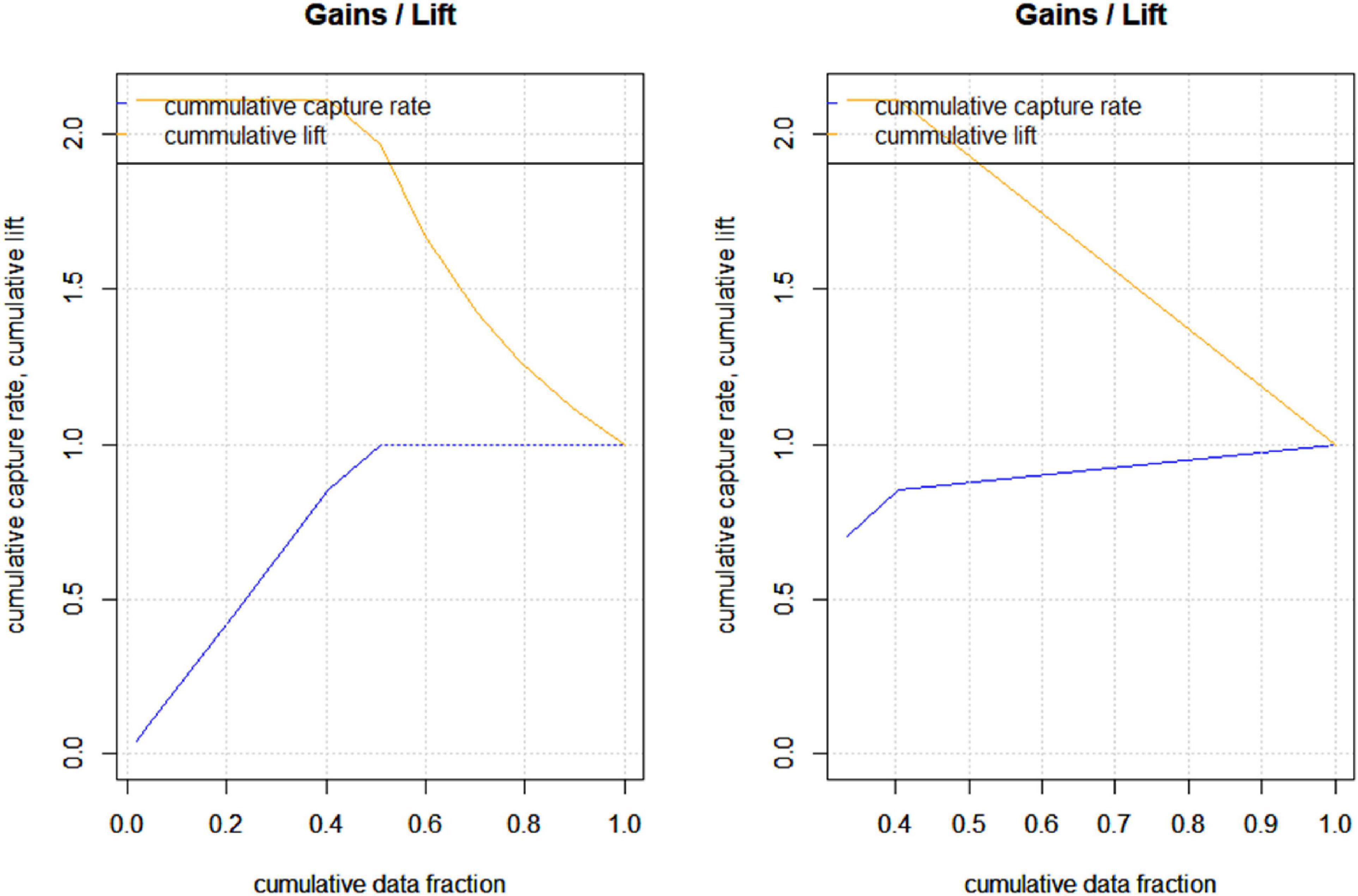
Figure 9. The gain and lift chart for explaining the performance of the model on the testing datasets for (A) DNN and (B) RF models.

Therefore, it is found that 20th DNN and 10th RF models are best model among 100 DNN and 132 RF models in terms of model fitness and prediction of new data. The optimized parameters for best DNN and RF models have been identified. For DNN model, the best parameters are as follows:

A total of five layers: one input, three hidden layers, one out layers; neurons: 713 for input, 50 for each hidden layer, and 2 for output layers; activation function: rectifierdropout for hidden layers, and softmax for output; regularization: l1 is 0.000010 for hidden and output layers; mean rate: 0.294 for hidden 1, 0.005 for hidden 2, 0.004 for hidden 3, and 0.0022 for output layer; rate rms: 0.448 for hidden 1, 0.003 for hidden 2, 0.007 for hidden 3, and 0.0007 for output; weight rms: 0.052 for hidden 1, 0.152 for hidden 2, 0.139 for hidden 3, and 0.779 for output; mean bias: 0.479 for hidden 1, 0.915 for hidden 2, 0.959 for hidden 3, and −0.013 for output layer.

On the other hand, the best parameters for best RF model are as follows:

Number of trees: 450; number of internal trees: 450; model size in bytes: 42517; min depth: 1; max depth: 2; mean depth: 1.0156; min leaves: 2; max leaves: 3; mean leaves: 2.01.

Understanding the factors that initiate landslides is crucial in preventing landslides and mitigating their impacts. The identification of these factors will allow for the development of effective strategies to tackle the problem. The current study has used machine learning techniques to identify the most influential parameters in the occurrence of landslides.

In the DNN model, the most influential parameters in the occurrence of landslides are rainfall, hillshade, soil texture, geology, NDVI, and elevation (Figure 10A). The occurrence of rainfall and its intensity is one of the most important factors in triggering landslides. The water content of soil increases when it rains, and this can cause instability in the soil structure. Hillshade, which refers to the angle and intensity of the sun’s rays on the land surface, affects the amount of solar radiation that is absorbed by the land surface. This, in turn, affects the rate of evaporation, which can also impact the stability of the soil. Soil texture and geology are also important parameters that can affect landslide occurrence. Certain types of soil and rock formations are more prone to landslides than others. NDVI, which is a measure of vegetation cover, can also affect the stability of the soil. Vegetation helps to stabilize the soil and reduce erosion.

FIGURE 10

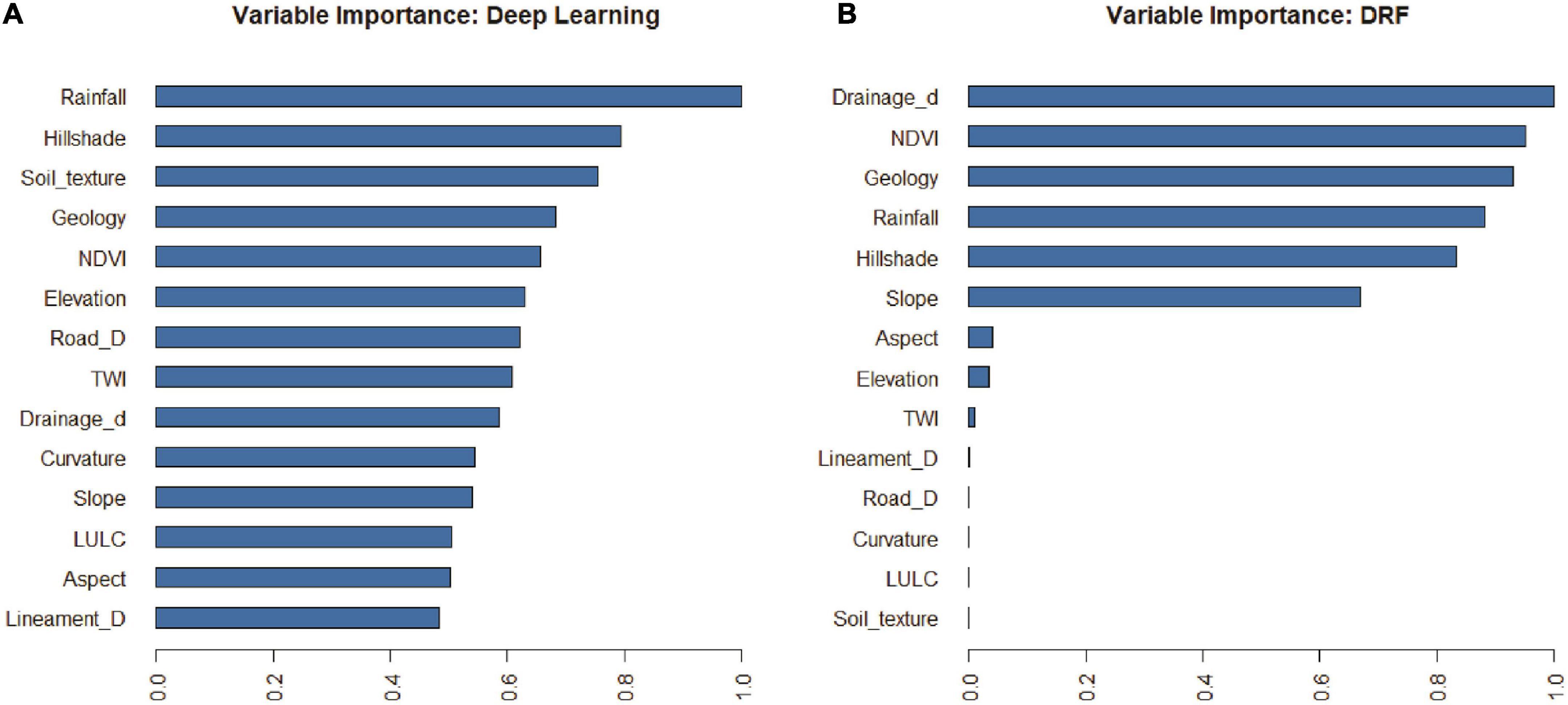
Figure 10. Computation of important parameter for predicting LSM using best (A) DNN, and (B) RF models.

In the RF model, the most influential parameters in the occurrence of landslides are drainage density, NDBI, geology, rainfall, and slope (Figure 10B). Drainage density refers to the amount of water flow in the land, and it can affect the stability of the soil. NDBI, which is a measure of the urbanization level of an area, can also impact the stability of the soil. The conversion of natural land to urban areas can cause soil erosion and instability. Geology and rainfall are also important factors that can affect landslide occurrence. As previously mentioned, certain types of soil and rock formations are more prone to landslides than others, and the occurrence of rainfall can trigger landslides. Finally, slope is another important factor in landslide occurrence. Steep slopes are more prone to landslides, and this parameter is commonly used in landslide susceptibility mapping.

In order to tackle these parameters, implementation strategies can be developed based on the identified influential factors. For example, to tackle the issue of rainfall, land-use planning can be conducted to ensure that development is not done in areas prone to landslides. To address the issue of steep slopes, slope stabilization techniques can be used, such as terracing or the planting of vegetation. Soil stabilization techniques can also be used to address soil texture and geology issues. Overall, the identification of influential parameters in the occurrence of landslides is critical to preventing landslides and mitigating their impact, and the implementation strategies can be developed based on the identified factors to reduce the risk of landslides.

3.5. Prediction of landslide susceptibility models

The best DNN and RF models have been implemented to raster datasets to generate the LSM at pixel scale. Then, the LSMs have been generated with values ranging from 0 to 1, where the value close to 1 indicates high susceptibility to landslide and vice versa. The generated LSMs have been classified into five classes using Jenk’s natural break algorithm, such as very high, high, moderate, low, and very low landslide susceptibility zone for DNN and RF (Figure 11). Then, we computed the areas under different LSM zones for DNN and RF models. It shows that 8.14 km² area predicted as very high LSM zone, followed by high (29.27 km²), moderate (47.86 km²), low (59.98 km²), and very low (57.06 km²) (Figure 11A). On the other hand, RF predicted 16.03 km² areas as very high LSM zone, followed by high (41.32 km²), moderate (61.45 km²), low (61.33 km²), and very low (18.4 km²) LSM zone (Figure 11B).

FIGURE 11

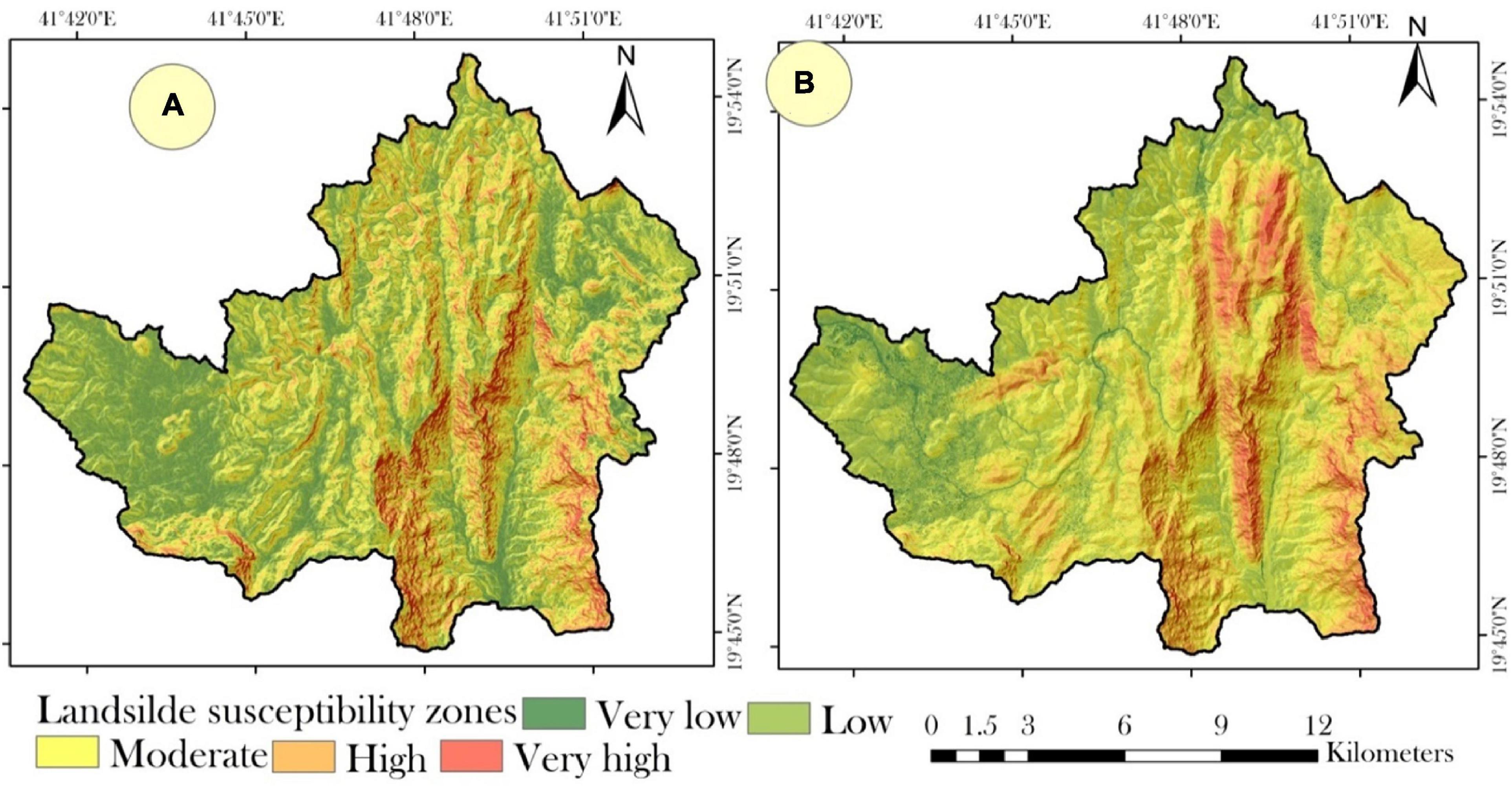
Figure 11. Landslide susceptibility mapping using (A) DNN and (B) RF models.

The results show the variation of areas under different LSM zones of DNN and RF models are relatively high for very high and very low landslide zones. The predicted high, moderate, low LSM zones have been visually screened and found that the predicted results are highly correlated with each other. Therefore, the results arises the question for reliability that planners and stakeholders will believe which models as there is variation between the models. To solve this issue, the resultant models have been validated with ground truth. The best model can be considered for management plans.

3.6. Model validation and comparisons

In this study, we used ROC curve, precision recall curve, F1, F2 score, gini, logloss, MSE, RMSE, and mean per class error. The accuracy assessment has been done using training and testing datasets for DNN and RF based LSMs. The AUC value of ROC curve for DNN model based on training dataset is 1, which indicates 100% accuracy of the model, while the AUC of precision recall curve is also 100%. The gini value with value ranging from 0 to 1, indicates the quality of a binary classifier, therefore, the value 0 shows the perfect equality, which can be considered totally useless classifier and vice versa. In this research, we obtained 1 gini value for DNN model, which considered that this model is perfect model for predicting LSM. The F1 and F2 value for the DNN model are 0.976 and 0.976, respectively. The higher the F1 and F2 values, the better the model. This DNN model can be considered a perfect model because of the F1 and F2 values. The mean per class rate is 0, while MSE, RMSE, and logloss are also very low, near 0, which indicates the performance of the DNN model based on training dataset is very high.

On the other hand, for RF based LSM model using training dataset, the AUC of ROC and precision recall curve are 1, while the gini value is 1. The F1 and F2 values are 0.99 and 0.991 for the RF model. The mean per class error is o, while the MSE, RMSE, and logloss are near 0. Therefore, these findings indicate that the performance of the model based on training data using RF model can be considered perfect and highly accurate model. However, the performance on training dataset does not count as accurate model, until the performance has been judge based on the testing dataset. If the model accurately predicts the new data, it can be considered as perfect and accurate model. Therefore, in this study, similar error matrices have been employed to evaluate the performance of the DNN and RF models based on testing dataset.

In this study, we computed AUC value for ROC and precision and recall curve for DNN and RF models based on testing dataset (Figure 12). Figures 12A, C show that the AUC value of DNN and RF are 0.962 and 0.935, indicating the very high agreement of the model with ground truth. In addition, the AUC of precision and recall curve for DNN and RF are 0.966 and 0.917, indicating higher area under the curve (AUC), which signifies the prediction is quite real (Figures 12B, D). In addition, the gini value is 0.923, F1 and F2 score are 0.963 and 0.984, mean per class error is still 0 for DNN model. The RMSE is 0.003, logloss is 0.0008, and the MSE is near 0 for DNN model. These findings indicate the DNN model can learn the new data and predict the LSM perfectly.

FIGURE 12

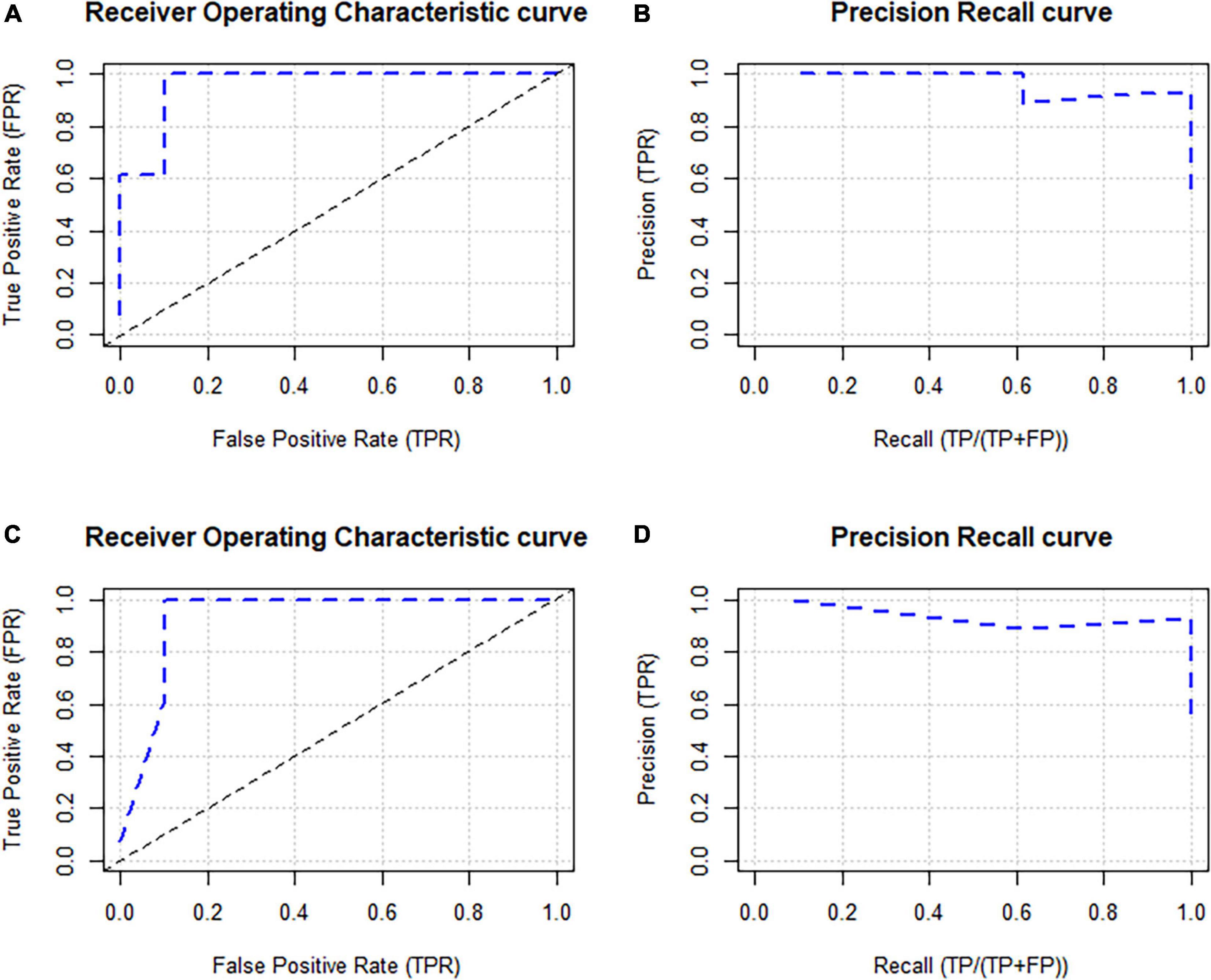
Figure 12. The accuracy assessment of susceptibility model using AUC of ROC curve and precision an recall curves for DNN (A,B) and RF (C,D).

On the other hand, the error matrices for RF model based on testing dataset show very high accuracy, such as 0.869 of gini value, 0.963 of F1, 0.984 of F2, 0.5 of mean per class error, 0.504 of logloss, 0.425 of RMSE, and 0.18 of MSE. These results show the satisfactory performance of the model.

However, we compare the DNN model with RF model as per the generated statistics of model evaluation, it is found that DNN model outperformed RF model. But it does not mean that RF model is not good performer, but it predicts LSM quite well. Therefore, it can be stated that RF model performed very well, but DNN performed better than RF model. As per this finding, the management plan should be DNN model oriented.

3.7. Sensitivity and uncertainty analysis

In the present study, DNN based sensitivity analysis has been performed to evaluate the sensitivity and uncertainty of the parameters to the output. The whole process has been implemented in the R programming language using several packages, such as “keras,” “tensorflow,” “Neuralsens,” and “monmlp.” For the modeling, the predicted LSM by DNN algorithm has been considered as the target variable; while the 12 landslide conditioning parameters have been considered as the input variables. In the present study, we chose DNN-predicted LSM as target because the model outperformed RF based model. However, we trained the DNN model using hyper-parameter tuning. In this study, the algorithm consists of five fully connected layers and dropout layers. The hyper-parameter tuning has been employed based on random search technique to find the best number of neurons (16, 32, 64, 128) and dropout rate (0.01, 0.02). We also used relu activation function for hidden layers, while sigmoid activation function has been used for output layers. In addition, we used adam algorithm for optimization. In the present study, we used cross entropy and accuracy matrices for plotting the accuracy assessment of the trained model. The matrices were plotted against each epoch for training and validation phases.

Figure 13 shows the variation of the accuracy with the number of epochs for the training and validation phases. It is found out that the error has been decreased rapidly in the first two epochs, showing that the network is learning fast. Afterward, the curves are getting flatten, which indicates the much epochs are not needed to train the model further. Therefore, the optimal model with 200 epochs was chosen. Moreover, since we have only a few data sets, the model took a long time to train. The whole procedure took almost 10 min.

FIGURE 13

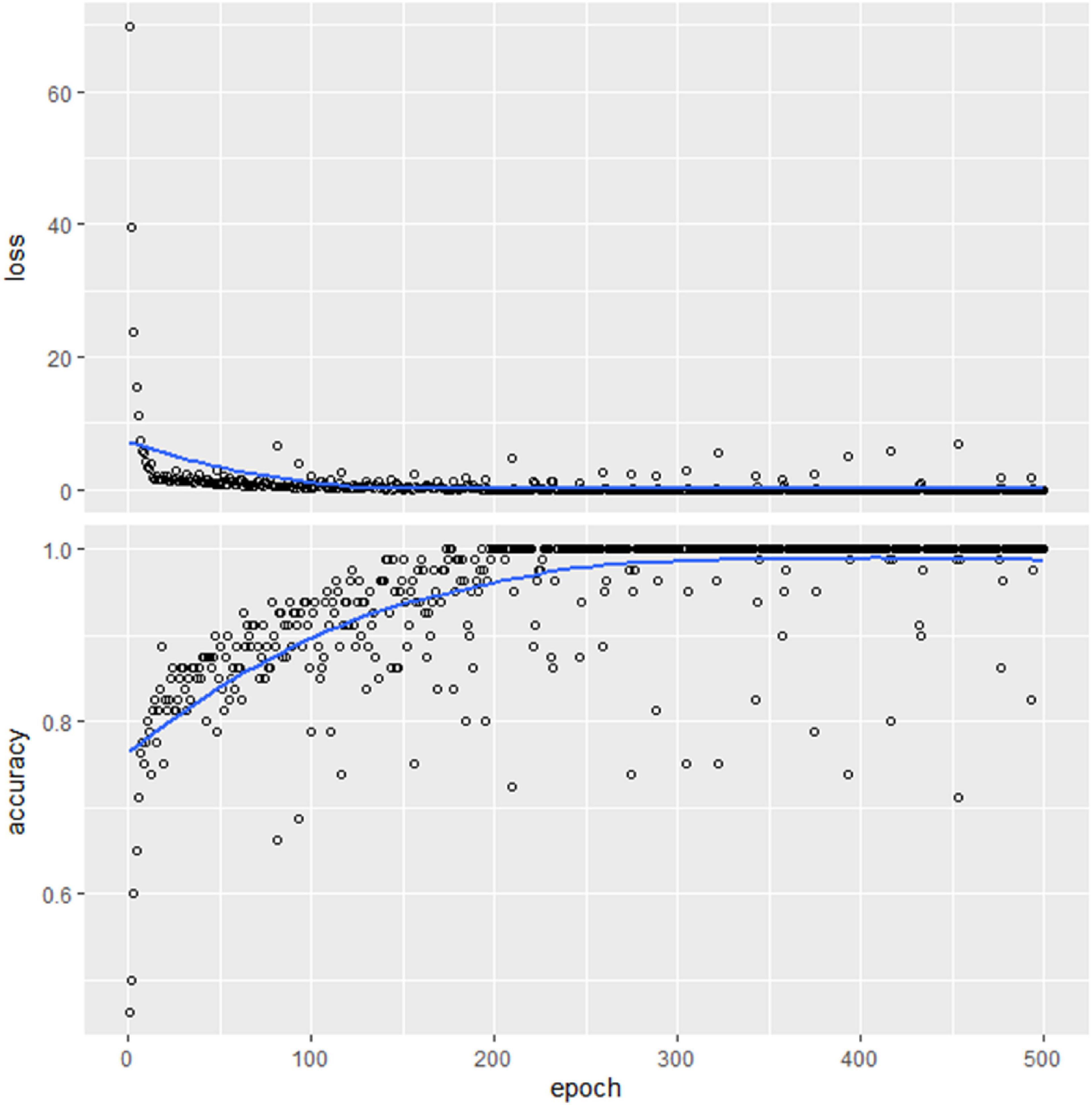
Figure 13. Training and validation accuracy changes with the number of epochs using DNN.

The sensitivity and uncertainty measures of input parameters and their effect on the output have been displayed using label plot, bar plot, and density plot in the present study (as shown in Figure 14). The label plot shows that TWI, curvature, LULC, hillshade, road density, and geology have negative non-linear relationships with LSM (Mean of sensitivity is <0, and variance of sensitivity is >0.01), whereas rainfall has a high positive non-linear relationship with LSM, followed by slope, soil texture, NDVI, drainage density, and lineament density. The bar plot shows the sensitivity measures of the importance of input parameters in relation to output parameters. Rainfall has the highest positive influence (0.6) in predicting landslide, followed by slope (0.5), soil texture (0.4), and other parameters, such as NDVI, drainage density, and elevation, have low positive influence (0.1). The same bar plot shows that TWI has the highest negative influence (0.55), followed by curvature (0.52), LULC (0.23), hillshade (0.18), and road density (0.1).

FIGURE 14

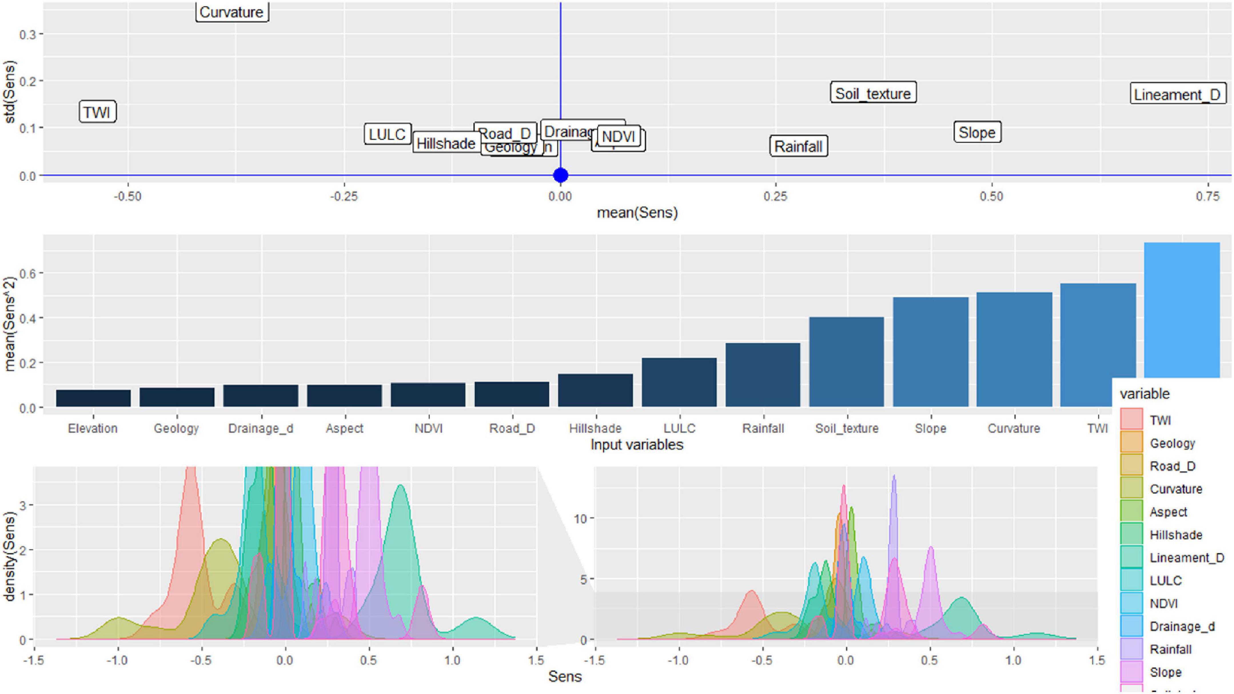
Figure 14. Sensitivity and uncertainty analysis using deep neural network based sensitivity technique.

It is evident from the findings that rainfall has a major impact on predicting landslide and that the sensitivity analysis should be conducted before initiating the management process. The uncertainty analysis emphasizes how the uncertainties of input parameters propagate to the output. The density plot displays the distribution pattern of input parameters and their linear and non-linear relationships with the output. The CV has been computed to show the variation in the data distribution pattern, and the higher the variation, the higher the uncertainty in the output variable. In this study, road density (−140.37%), followed by geology (−113.8%), and hillshade (−53.13%) have a high CV, and therefore, they need to be normalized and preprocessed before using them for model building to avoid erroneous results. It can be concluded that the rainfall should be closely monitored and the threshold value for rainfall that can initiate a landslide should be identified to use it as an early warning system.

After identification of sensitive and uncertain parameters, the contribution of the value of each sample on the LSM prediction can provide further information, which may be very useful for management plans. Figure 15 shows the contribution of each sample of input parameters to the landslide. The influence of sample has been indicated by high and low value with blue to orange color. The shade toward deep blue indicates high influence, while the shades toward orange indicate low influence. The soil texture, slope, rainfall, NDVI, and aspect have positive influence, while some parts of drainage density, NDVI, hillshade, curvature, road density, geology have positively influence the LSM. In addition, some parts of curvature, elevation, LULC, hillshade, TWI, and geology negatively influence the LSM.

FIGURE 15

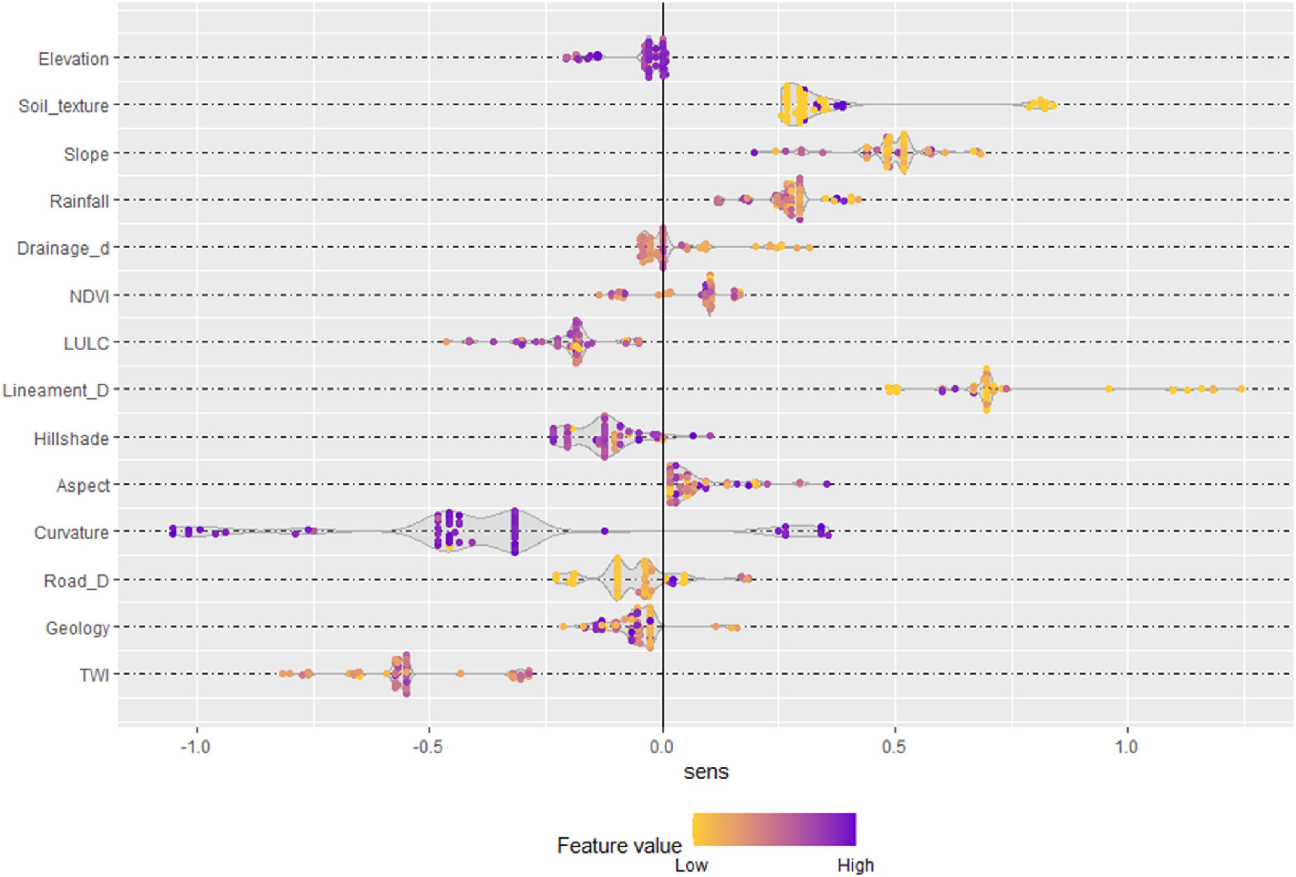
Figure 15. The influence of value of each sample of input parameters to the LSM.

4. Discussion

Effective planning and development of hilly and mountainous regions requires special consideration due to the presence of natural hazards, with landslides being one of the most significant risks (Pourghasemi et al., 2012; Kirschbaum et al., 2015). Landslide susceptibility studies are essential in these areas to provide decision-makers and planners with an initial proactive approach (Youssef et al., 2015; Abbaszadeh Shahri et al., 2019; Ali et al., 2021). However, creating accurate models for landslide susceptibility is a major challenge that requires the selection of appropriate factors and models (Mallick et al., 2021; Mandal et al., 2021; Hakim et al., 2022; Sun et al., 2022).

Landslide indicators vary depending on the characteristics of the area and are related to various environmental and anthropogenic factors (Youssef et al., 2015). Selecting the appropriate and most influential factors is important for accurate landslide susceptibility evaluation (Ali et al., 2021). In order to achieve this, various techniques such as multicollinearity tests have been used to identify relationships among landslide indicators that could negatively impact the overall accuracy of the model (Mallick et al., 2021). Multicollinearity tests were performed to ensure that there was no correlation among the selected factors (Mallick et al., 2021). All factors were incorporated into the models as a result (Mallick et al., 2021). In this study, multicollinearity as well as RFE and information gain ratio was used for selecting appropriate parameters. We used the VIF test to evaluate multicollinearity between LIFs and found no significant correlation among the selected factors. Rainfall, Slope, Curvature, Elevation, and Hillshade were found to be the most important factors in predicting landslide susceptibility in the area. The importance of these factors was determined using variable importance analysis, which ranked the 14 variables based on their significance in the model.

These findings indicate that all selected parameters have a significant impact on landslide susceptibility. While selecting the appropriate landslide indicators is crucial, the diversity of indicators and characteristics of the area make it challenging to establish clear rules for selection. Nonetheless, the study suggests that the selection of appropriate indicators can be achieved by testing multicollinearity and employing variable importance analysis.

Machine learning and deep learning techniques are effective in handling complex, non-linear datasets and identifying hidden patterns within the data to predict outputs with high accuracy (Shrestha et al., 2017; Ma and Mei, 2021; Mandal et al., 2021; Shahabi et al., 2021; Hakim et al., 2022; Sun et al., 2022). However, the performance of these models is heavily dependent on the availability of field data for training, and limited data can negatively impact the predictive skills of the models (Mandal et al., 2021). To address this challenge, various techniques have been developed around the world, including the application of hyper-tuned RF and DNN algorithms under the open-source H₂O framework. In this research, we have used these algorithms to construct accurate models of landslide susceptibility, which can help identify landslide-prone areas.

The study evaluates the performance of RF and DNN models using the area under the receiver operating characteristic curve (AUC-ROC) for validation. Although both models achieved satisfactory accuracy (AUC > 0.80), the DNN model outperformed the RF model in landslide susceptibility mapping. Previous research has demonstrated that the RF method is an effective tool for identifying areas where landslides are likely to occur using spatial data (Xu et al., 2012; Lagomarsino et al., 2017; Shrestha et al., 2017; Pham et al., 2019). In recent years, the DNN model has become increasingly popular among researchers studying landslide susceptibility (Xiao et al., 2018; Ghorbanzadeh et al., 2019). Wang et al. (2019) reported that the DNN framework achieved higher or comparable prediction accuracy, and this study also corroborates their findings (Ciregan et al., 2012; Krizhevsky et al., 2017; Dou et al., 2020). Consequently, DNN has the potential to provide more accurate predictions and to enhance our comprehension of areas prone to landslides. Therefore, the study shows that fine-tuned models can improve performance in data-scarce conditions.

One of the recent studies suggests that the DNN model performs better than other algorithms, such as CNN, LSTM, and RNN, in predicting landslide susceptibility (Habumugisha et al., 2022). However, these other algorithms can still be used as they perform similarly to the DNN model (Habumugisha et al., 2022). Previous research also supports the effectiveness of the DNN model in predicting landslide susceptibility (Ciregan et al., 2012; Krizhevsky et al., 2017; Xiao et al., 2018; Ghorbanzadeh et al., 2019; Dou et al., 2020). Overall, the study suggests that the DNN model can provide better predictions and improve understanding of landslide-susceptibility areas.

However, this study shows that more than half of the study area falls under very low and low LS zones, while nearly 20% area falls under the very high and high LS zones. This finding is identical to the finding of Mallick et al. (2021) who also found about 25% of the total area of Asir region under high and very high LS zones. Further, the study shows that the LS is comparatively high in the southern and south-eastern parts of Aqabat Al-Sulbat Asir region while most of the western and northern parts have either low or very low LS. This is possible due to gentle slope, low elevation variation and strong geological setting in the western and northern parts. Further, central parts of the Aqabat Al-Sulbat Asir region also have high LS because in this part, the terrain is mostly hilly with very high drainage and lineament density which triggers the risk of landslide.

The findings of the study using DNN-based sensitivity analysis for landslide susceptibility assessment have important implications for landslide management. The sensitivity analysis provides a clear understanding of the influence of input parameters on the output, which can be used to prioritize management interventions and improve the effectiveness of landslide risk reduction measures. By identifying the most important input parameters, resources and efforts can be focused on those parameters, resulting in more effective management interventions.

The use of DNN for sensitivity analysis in landslide susceptibility assessment is a significant Contribution To The Field. While previous methods such as Sobol, Efast, and Monte Carlo simulation have been used for sensitivity analysis, the use of DNN provides a more efficient and accurate approach for analyzing large datasets with numerous input parameters. This is particularly important in the context of landslide susceptibility assessment, where there are often many potential input parameters that need to be considered. The use of DNN-based sensitivity analysis allows for more precise and targeted management interventions, which can lead to better outcomes in terms of reducing landslide risk and protecting communities and infrastructure.

The results of this study can help in landslide management by providing a better understanding of the key input parameters that influence landslide susceptibility. This can inform targeted management interventions, such as to control LSM or reduce the impact of landslide, the rainfall should be closely monitored and also need to do measure the threshold value for rainfall which can initiate the landslide, can be used as early warning system. The sensitivity analysis also allows for the identification of input parameters that may require normalization or preprocessing before being used for model building. This can prevent erroneous results and improve the accuracy of landslide susceptibility predictions. Overall, this study provides a valuable Contribution To The Field of landslide susceptibility assessment and can have important implications for the management of landslide risk.

In this study, we have explored variables that can contribute to landslides, and identified methods that can be applied for landslide susceptibility mapping in areas beyond the study site. The use of hyper-tuned RF and DNN models under an open-source H₂O framework is a novel approach in Saudi Arabia, and coupling these models with spatial analytical methods for landslide susceptibility modeling is a valuable consideration.

The comparison of the performance of the two hyper-tuned models is also a valuable Contribution To The Field, as it provides insights into which model may be better suited for different types of data and situations. Additionally, the authors propose a novel DNN model for sensitivity analysis that examines how triggers behave in causing landslides, which is an important step toward understanding the causes and predicting the occurrence of landslides.

The application of these methods and models has significant potential societal outcomes, as landslides can have devastating impacts on communities, infrastructure, and the environment. By improving our ability to predict and map landslide susceptibility, we can take proactive measures to mitigate the risks and reduce the impacts of landslides. This can include implementing early warning systems, developing hazard maps, and identifying areas that may be at high risk for landslides.

5. Conclusion

This study explores the use of machine learning models such as RF and DNN for predicting landslide susceptibility. The models were hypertuned using a grid search technique to determine the best model for the task, and a DNN-based sensitivity and uncertainty analysis was conducted to identify the most sensitive and uncertain parameters involved. The results provide valuable insights into model hypertuning and sensitivity and uncertainty analysis, with the DNN-based analysis being a novel approach in natural hazard research.

The grid search method produced 100 DNN models and 132 RF models, and the 20th DNN model and 10th RF model were identified as the baseline models for predicting landslides. The analysis showed that the models predicted high and very high landslide susceptibility zones, covering 35.1–41.32 and 15.14–16.2 km², respectively. Both models achieved a high level of accuracy with an AUC score of >0.9, indicating their robust performance. However, the DNN model outperformed the RF model. Sensitivity analysis revealed that rainfall, slope, aspect and LULC were the most sensitive parameters in predicting landslide susceptibility, while geology was identified as the most uncertain parameter. Therefore, special attention should be paid to normalizing or pre-processing these uncertain parameters to avoid erroneous results.

This study provides valuable scientific insights into landslide prediction analysis, although there are some limitations that need to be addressed in future research. Firstly, the number of parameters involved is quite low, given the complexity of landslides, so increasing the number of parameters could yield more accurate results. Additionally, field surveys for landslide locations need to be expanded to improve the accuracy of landslide predictions, and the use of high-resolution images could also improve the results significantly. Nevertheless, these findings can aid stakeholders in selecting the best model and identifying the most sensitive and uncertain parameters to propose robust management plans.

Data availability statement

The raw data supporting the conclusions of this article will be made available by the authors, without undue reservation.

Author contributions

MD and JM: conceptualization. JM: data curation, investigation, software, and validation. MD, JM, and SA: formal analysis. SA: funding acquisition and writing—review and editing. JM and SA: methodology and writing—original draft. SA and MD: project administration. MD: resources, supervision, and visualization. All authors contributed to the article and approved the submitted version.

Funding

Funding for this research was given under award number: RGP2/185/43 by the Deanship of Scientific Research; King Khalid University, Ministry of Education, Saudi Arabia.

Acknowledgments

We extend their appreciation to the Deanship of Scientific Research at King Khalid University for funding this work through Research Group under grant number: RGP2/185/43. We are also thankful to the USGS Earth Explorer for making the satellite data freely available.

Conflict of interest

The authors declare that the research was conducted in the absence of any commercial or financial relationships that could be construed as a potential conflict of interest.

Publisher’s note

All claims expressed in this article are solely those of the authors and do not necessarily represent those of their affiliated organizations, or those of the publisher, the editors and the reviewers. Any product that may be evaluated in this article, or claim that may be made by its manufacturer, is not guaranteed or endorsed by the publisher.

Footnotes

1. ^ https://earthexplorer.usgs.gov/

References

Abbaszadeh Shahri, A., Spross, J., Johansson, F., and Larsson, S. (2019). Landslide susceptibility hazard map in southwest Sweden using artificial neural network. Catena 183:104225. doi: 10.1016/j.catena.2019.104225

CrossRef Full Text | Google Scholar

Achu, A. L., Gopinath, G., and Surendran, U. (2021). “Landslide susceptibility modelling using deep-learning and machine-learning methods-A study from southern Western Ghats, India,” in 2021 IEEE international India geoscience and remote sensing symposium (InGARSS), (Piscataway, NJ: IEEE), 360–364. doi: 10.1109/InGARSS51564.2021.9792034

CrossRef Full Text | Google Scholar

Ali, S. A., Parvin, F., Vojteková, J., Costache, R., Linh, N. T. T., Pham, Q. B., et al. (2021). GIS-based landslide susceptibility modeling: A comparison between fuzzy multi-criteria and machine learning algorithms. Geosci. Front. 12, 857–876. doi: 10.1016/j.gsf.2020.09.004

CrossRef Full Text | Google Scholar

Alqadhi, S., Mallick, J., Talukdar, S., Bindajam, A. A., Van Hong, N., and Saha, T. K. (2021). Selecting optimal conditioning parameters for landslide susceptibility: An experimental research on Aqabat Al-Sulbat, Saudi Arabia. Environ. Sci. Pollut. Res. 29, 3743–3762. doi: 10.1007/s11356-021-15886-z

PubMed Abstract | CrossRef Full Text | Google Scholar

Alqahtani, A., Shah, M. I., Aldrees, A., and Javed, M. F. (2022). Comparative assessment of individual and ensemble machine learning models for efficient analysis of river water quality. Sustainability 14:1183. doi: 10.3390/su14031183

CrossRef Full Text | Google Scholar

Arabameri, A., Chandra Pal, S., Rezaie, F., Chakrabortty, R., Saha, A., Blaschke, T., et al. (2021). Decision tree based ensemble machine learning approaches for landslide susceptibility mapping. Geocarto Int. 37, 4594–4627. doi: 10.1080/10106049.2021.1892210

CrossRef Full Text | Google Scholar

Azarafza, M., Azarafza, M., Akgün, H., Atkinson, P. M., and Derakhshani, R. (2021). Deep learning-based landslide susceptibility mapping. Sci. Rep. 11:24112. doi: 10.1038/s41598-021-03585-1

PubMed Abstract | CrossRef Full Text | Google Scholar

Benbouras, M. A. (2022). Hybrid meta-heuristic machine learning methods applied to landslide susceptibility mapping in the Sahel-Algiers. Int. J. Sediment Res. 37, 601–618.

Google Scholar

Breiman, L. (2001). Random forests. Mach. Learn. 45, 5–32. doi: 10.1023/A:1010933404324

CrossRef Full Text | Google Scholar

Bui, D. T., Khosravi, K., Tiefenbacher, J., Nguyen, H., and Kazakis, N. (2020). Improving prediction of water quality indices using novel hybrid machine-learning algorithms. Sci. Total Environ. 721:137612. doi: 10.1016/j.scitotenv.2020.137612

PubMed Abstract | CrossRef Full Text | Google Scholar

Ciregan, D., Meier, U., and Schmidhuber, J. (2012). “Multi-column deep neural networks for image classification,” in Proceedings of the IEEE computer society conference on computer vision and pattern recognition, (Piscataway, NJ: IEEE). doi: 10.1109/EMBC46164.2021.9630183

PubMed Abstract | CrossRef Full Text | Google Scholar

Costache, R., Trung Tin, T., Arabameri, A., Crãciun, A., Ajin, R. S., Costache, I., et al. (2022). Flash-flood hazard using deep learning based on H₂O R package and fuzzy-multicriteria decision-making analysis. J. Hydrol. 609:127747. doi: 10.1016/j.jhydrol.2022.127747

CrossRef Full Text | Google Scholar

Das, S., Sarkar, S., and Kanungo, D. P. (2022). A critical review on landslide susceptibility zonation: Recent trends, techniques, and practices in Indian Himalaya. Nat. Hazards 115, 23–72. doi: 10.1007/s11069-022-05554-x

CrossRef Full Text | Google Scholar

Daviran, M., Shamekhi, M., Ghezelbash, R., and Maghsoudi, A. (2022). Landslide susceptibility prediction using artificial neural networks, SVMs and random forest: Hyperparameters tuning by genetic optimization algorithm. Int. J. Environ. Sci. Technol. 20, 259–276. doi: 10.1007/s13762-022-04491-3

CrossRef Full Text | Google Scholar

Dela, A., Shtylla, B., and de Pillis, L. (2022). Multi-method global sensitivity analysis of mathematical models. J. Theor. Biol. 546:111159. doi: 10.1016/j.jtbi.2022.111159

PubMed Abstract | CrossRef Full Text | Google Scholar

Deng, H., Wu, X., Zhang, W., Liu, Y., Li, W., Li, X., et al. (2022). Slope-unit scale landslide susceptibility mapping based on the random forest model in deep valley areas. Remote Sens. 14:4245. doi: 10.3390/rs14174245

CrossRef Full Text | Google Scholar

Dou, J., Yunus, A. P., Merghadi, A., Shirzadi, A., Nguyen, H., Hussain, Y., et al. (2020). Different sampling strategies for predicting landslide susceptibilities are deemed less consequential with deep learning. Sci. Total Environ. 720:137320. doi: 10.1016/j.scitotenv.2020.137320

PubMed Abstract | CrossRef Full Text | Google Scholar

Garcia, D., Arostegui, I., and Prellezo, R. (2019). Robust combination of the Morris and Sobol methods in complex multidimensional models. Environ. Model. Softw. 122:104517. doi: 10.1016/j.envsoft.2019.104517

CrossRef Full Text | Google Scholar

Gautam, P., Kubota, T., Sapkota, L. M., and Shinohara, Y. (2021). Landslide susceptibility mapping with GIS in high mountain area of Nepal: A comparison of four methods. Environ. Earth Sci. 80:359. doi: 10.1007/s12665-021-09650-2

CrossRef Full Text | Google Scholar

Gavrishchaka, V., Yang, Z., Miao, R., and Senyukova, O. (2018). Advantages of hybrid deep learning frameworks in applications with limited data. Int. J. Machine Learn. Comput. 8, 549–558. doi: 10.3390/s22239500

PubMed Abstract | CrossRef Full Text | Google Scholar

Ghorbanzadeh, O., Blaschke, T., Gholamn, K., Meena, S. R., Tiede, D., and Aryal, J. (2019). Evaluation of different machine learning methods and deep-learning convolutional neural networks for landslide detection. Remote Sens. 11:196. doi: 10.3390/rs11020196

CrossRef Full Text | Google Scholar

Glen, G., and Isaacs, K. (2012). Estimating Sobol sensitivity indices using correlations. Environ. Model. Softw. 37, 157–166. doi: 10.1016/j.envsoft.2012.03.014

CrossRef Full Text | Google Scholar

Gunturu, V. R. (2022). “GIS, remote sensing and drones for disaster risk management,” in 5th world congress on disaster management, ed. S. A. Babu (Oxford: Routledge), 182–194. doi: 10.4324/9781003341956-26

PubMed Abstract | CrossRef Full Text | Google Scholar

Habumugisha, J. M., Chen, N., Rahman, M., Islam, M. M., Ahmad, H., Elbeltagi, A., et al. (2022). Landslide susceptibility mapping with deep learning algorithms. Sustainability 14:1734.

Google Scholar

Hakim, W. L., Rezaie, F., Nur, A. S., Panahi, M., Khosravi, K., Lee, C. W., et al. (2022). Convolutional neural network (CNN) with metaheuristic optimization algorithms for landslide susceptibility mapping in Icheon, South Korea. J. Environ. Manag. 305:114367. doi: 10.1016/j.jenvman.2021.114367

PubMed Abstract | CrossRef Full Text | Google Scholar

Hsieh, N. H., Reisfeld, B., Bois, F. Y., and Chiu, W. A. (2018). Applying a global sensitivity analysis workflow to improve the computational efficiencies in physiologically-based pharmacokinetic modeling. Front. Pharmacol. 9:588. doi: 10.3389/fphar.2018.00588

PubMed Abstract | CrossRef Full Text | Google Scholar

Huang, Y., and Zhao, L. (2018). Review on landslide susceptibility mapping using support vector machines. Catena 165, 520–529. doi: 10.1016/j.catena.2018.03.003

CrossRef Full Text | Google Scholar

Ibrahim, K. S. M. H., Huang, Y. F., Ahmed, A. N., Koo, C. H., and El-Shafie, A. (2022). A review of the hybrid artificial intelligence and optimization modelling of hydrological streamflow forecasting. Alexandria Eng. J. 61, 279–303. doi: 10.1016/j.aej.2021.04.100

CrossRef Full Text | Google Scholar

Jaxa-Rozen, M., and Kwakkel, J. (2018). Tree-based ensemble methods for sensitivity analysis of environmental models: A performance comparison with Sobol and Morris techniques. Environ. Model. Softw. 107, 245–266. doi: 10.1016/j.envsoft.2018.06.011

CrossRef Full Text | Google Scholar

Kavzoglu, T., and Teke, A. (2022). Predictive performances of ensemble machine learning algorithms in landslide susceptibility mapping using random forest, extreme gradient boosting (XGBoost) and natural gradient boosting (NGBoost). Arab. J. Sci. Eng. 47, 7367–7385. doi: 10.1007/s13369-022-06560-8

CrossRef Full Text | Google Scholar

Kirschbaum, D., Stanley, T., and Yatheendradas, S. (2015). Modeling landslide susceptibility over large regions with fuzzy overlay. Landslides 13, 485–496. doi: 10.1007/s10346-015-0577-2

CrossRef Full Text | Google Scholar

Krizhevsky, A., Sutskever, I., and Hinton, G. E. (2017). ImageNet classification with deep convolutional neural networks. Commun. ACM 60, 84–90. doi: 10.1145/3065386

CrossRef Full Text | Google Scholar

Lagomarsino, D., Tofani, V., Segoni, S., Catani, F., and Casagli, N. A. (2017). Tool for classification and regression using random forest methodology: Applications to landslide susceptibility mapping and soil thickness modeling. Environ. Model. Assess. 22, 201–214. doi: 10.1007/s10666-016-9538-y

CrossRef Full Text | Google Scholar

Lee, S., and Min, K. (2001). Statistical analysis of landslide susceptibility at Yongin, Korea. Environ. Geol. 40, 1095–1113. doi: 10.1007/s002540100310

CrossRef Full Text | Google Scholar

Leonardi, G., Palamara, R., and Suraci, F. (2020). A fuzzy methodology to evaluate the landslide risk in road lifelines. Transp. Res. Proc. 45, 732–739. doi: 10.1016/j.trpro.2020.02.104

CrossRef Full Text | Google Scholar

Li, Y., Wang, Y., Sun, Y., Li, J., Li, Y., Wang, Y., et al. (2022). Global sensitivity analysis of the LPJ model for larix olgensis Henry forests NPP in Jilin Province, China. Forests 13:874. doi: 10.3390/f13060874

CrossRef Full Text | Google Scholar

Liu, W., and Ding, L. (2020). Global sensitivity analysis of influential parameters for excavation stability of metro tunnel. Autom. Constr. 113:103080. doi: 10.1016/j.autcon.2020.103080

CrossRef Full Text | Google Scholar

Loche, M., Alvioli, M., Marchesini, I., Bakka, H., and Lombardo, L. (2022). Landslide susceptibility maps of Italy: Lesson learnt from dealing with multiple landslide types and the uneven spatial distribution of the national inventory. Earth Sci. Rev. 232:104125.

Google Scholar

Ma, Z., and Mei, G. (2021). Deep learning for geological hazards analysis: Data, models, applications, and opportunities. Earth Sci. Rev. 223:103858.

Google Scholar

Mallick, J., Alqadhi, S., Talukdar, S., Alsubih, M., Ahmed, M., Khan, R. A., et al. (2021). Risk assessment of resources exposed to rainfall induced landslide with the development of GIS and RS based ensemble metaheuristic machine learning algorithms. Sustainability 13:457.

Google Scholar

Mandal, K., Saha, S., and Mandal, S. (2021). Applying deep learning and benchmark machine learning algorithms for landslide susceptibility modelling in Rorachu river basin of Sikkim Himalaya, India. Geosci. Front. 12:101203. doi: 10.1016/j.gsf.2021.101203

CrossRef Full Text | Google Scholar

Mantovani, M., Bossi, G., Dykes, A. P., Pasuto, A., Soldati, M., and Devoto, S. (2022). Coupling long-term GNSS monitoring and numerical modelling of lateral spreading for hazard assessment purposes. Eng. Geol. 296:106466.

Google Scholar

Mehrabi, M. (2021). Landslide susceptibility zonation using statistical and machine learning approaches in Northern Lecco, Italy. Nat. Hazards 111, 901–937.

Google Scholar

Mezősi, G. (2022). Geophysical hazards. Natural hazards mitigation and their impact. Springer International Publishing, 35–96. Available online at: https://doi.org/10.1007/978-3-031-07226-0_2

Google Scholar

Naikoo, M. W., Rihan, M., Shahfahad, Peer, A. H., Talukdar, S., Mallick, J., et al. (2022). Analysis of peri-urban land use/land cover change and its drivers using geospatial techniques and geographically weighted regression. Environ. Sci. Pollut. Res. 2022, 1–19. doi: 10.1007/s11356-022-18853-4

PubMed Abstract | CrossRef Full Text | Google Scholar

Nath, R. R., Sharma, M. L., Goswami, A., Sweta, K., and Pareek, N. (2021). Landslide susceptibility zonation with special emphasis on tectonic features for occurrence of landslides in lower Indian Himalaya. J. Indian Soc. Remote Sens. 49, 1221–1238.

Google Scholar

Nhu, V. H., Shirzadi, A., Shahabi, H., Chen, W., Clague, J. J., Geertsema, M., et al. (2020). Shallow landslide susceptibility mapping by random forest base classifier and its ensembles in a semi-arid region of Iran. Forests 11:421.

Google Scholar

Orhan, O., Bilgilioglu, S. S., Kaya, Z., Ozcan, A. K., and Bilgilioglu, H. (2020). Assessing and mapping landslide susceptibility using different machine learning methods. Geocarto Int. 37, 2795–2820.

Google Scholar

Pham, B. T., Prakash, I., Singh, S. K., Shirzadi, A., Shahabi, H., Tran, T.-T.-T., et al. (2019). Landslide susceptibility modeling using reduced error pruning trees and different ensemble techniques: Hybrid machine learning approaches. Catena 175, 203–218.

Google Scholar

Pham, B. T., Van Phong, T., Nguyen-Thoi, T., Parial, K., Singh, S., Ly, H. B., et al. (2020). Ensemble modeling of landslide susceptibility using random subspace learner and different decision tree classifiers. Geocarto Int. 37, 735–757.

Google Scholar

Pourghasemi, H. R., Pradhan, B., and Gokceoglu, C. (2012). Application of fuzzy logic and analytical hierarchy process (AHP) to landslide susceptibility mapping at Haraz watershed. Iran. Nat. Hazards 63, 965–996.

Google Scholar

Prasad, D. V. V., Venkataramana, L. Y., Kumar, P. S., Prasannamedha, G., Harshana, S., Srividya, S. J., et al. (2022). Analysis and prediction of water quality using deep learning and auto deep learning techniques. Sci. Total Environ. 821:153311.

Google Scholar

Remondo, J., Bonachea, J., and Cendrero, A. (2008). Quantitative landslide risk assessment and mapping on the basis of recent occurrences. Geomorphology 94, 496–507.

Google Scholar

Roy, J., Saha, S., Arabameri, A., Blaschke, T., and Bui, D. T. (2019). A novel ensemble approach for landslide susceptibility mapping (LSM) in Darjeeling and Kalimpong Districts, West Bengal, India. Remote Sens. 11:2866.

Google Scholar

Saha, S., Roy, J., Pradhan, B., and Hembram, T. K. (2021). Hybrid ensemble machine learning approaches for landslide susceptibility mapping using different sampling ratios at East Sikkim Himalayan, India. Adv. Space Res. 68, 2819–2840.

Google Scholar

Saha, S., Saha, A., Hembram, T. K., Kundu, B., and Sarkar, R. (2022). Novel ensemble of deep learning neural network and support vector machine for landslide susceptibility mapping in Tehri region, Garhwal Himalaya. Geocarto Int. doi: 10.1080/10106049.2022.2120638

CrossRef Full Text | Google Scholar

Shahabi, H., Shirzadi, A., Ronoud, S., Asadi, S., Pham, B. T., Mansouripour, F., et al. (2021). Flash flood susceptibility mapping using a novel deep learning model based on deep belief network, back propagation and genetic algorithm. Geosci. Front. 12:101100. doi: 10.1016/j.gsf.2020.10.007

CrossRef Full Text | Google Scholar

Shang, K., Yao, Y., Liang, S., Zhang, Y., Fisher, J. B., Chen, J., et al. (2021). A deep neural networks method to integrate satellite-derived evapotranspiration products, eddy covariance observations and ancillary information. Agric. For. Meteorol. 308:108582.

Google Scholar

Shrestha, S., Kang, T.-S., and Suwal, M. (2017). An ensemble model for co-seismic landslide susceptibility using GIS and random forest method. ISPRS Int. J. Geo Inf. 6:365.

Google Scholar

Song, C., Yao, L., Hua, C., and Ni, Q. (2021). A water quality prediction model based on variational mode decomposition and the least squares support vector machine optimized by the sparrow search algorithm (VMD-SSA-LSSVM) of the Yangtze River, China. Environ. Monit. Assess. 193:363. doi: 10.1007/s10661-021-09127-6

PubMed Abstract | CrossRef Full Text | Google Scholar

Sun, Y., Zhang, F., Lin, H., and Xu, S. A. (2022). Forest fire susceptibility modeling approach based on light gradient boosting machine algorithm. Remote Sens. 14:4362.

Google Scholar

Sweta, K., Goswami, A., Nath, R. R., and Bahuguna, I. M. (2022). Performance assessment for three statistical models of landslide susceptibility zonation mapping: A case study for Dharamshala Region, Himachal Pradesh, India. J. Earth Syst. Sci. 131:143.

Google Scholar

Talukdar, S., Eibek, K. U., Akhter, S., Ziaul, S., Towfiqul Islam, A. R. M., and Mallick, J. (2021). Modeling fragmentation probability of land-use and land-cover using the bagging, random forest and random subspace in the Teesta River Basin, Bangladesh. Ecol. Indic. 126:107612.

Google Scholar

Tang, X., Li, J., Liu, M., Liu, W., and Hong, H. (2020). Flood susceptibility assessment based on a novel random Naïve Bayes method: A comparison between different factor discretization methods. Catena 190:104536.

Google Scholar

Tanyu, B. F., Abbaspour, A., Alimohammadlou, Y., and Tecuci, G. (2021). Landslide susceptibility analyses using random forest, C4.5, and C5.0 with balanced and unbalanced datasets. Catena 203:105355.

Google Scholar

Tien Bui, D., Hoang, N.-D., Martínez-Álvarez, F., Ngo, P.-T. T., Hoa, P. V., Pham, T. D., et al. (2020). A novel deep learning neural network approach for predicting flash flood susceptibility: A case study at a high frequency tropical storm area. Sci. Total Environ. 701:134413. doi: 10.1016/j.scitotenv.2019.134413

PubMed Abstract | CrossRef Full Text | Google Scholar

Wang, Y., Fang, Z., and Hong, H. (2019). Comparison of convolutional neural networks for landslide susceptibility mapping in Yanshan County, China. Sci. Total Environ. 666, 975–993. doi: 10.1016/j.scitotenv.2019.02.263

PubMed Abstract | CrossRef Full Text | Google Scholar

World Bank (2005). “Natural disaster hotspots: A global risk analysis,” in Disaster management series, the international bank for reconstruction and development, eds M. Dilley, R. Chen, U. Deichmann, L. Arthur, A. Lerner-Lam, and M. Arnold (Washington, DC: The World Bank).

Google Scholar

Xi, C., Han, M., Hu, X., Liu, B., He, K., Luo, G., et al. (2022). Effectiveness of Newmark-based sampling strategy for coseismic landslide susceptibility mapping using deep learning, support vector machine, and logistic regression. Bull. Eng. Geol. Environ. 81:174.

Google Scholar

Xiao, L., Zhang, Y., and Peng, G. (2018). Landslide susceptibility assessment using integrated deep learning algorithm along the china-nepal highway. Sensors 18:4436. doi: 10.3390/s18124436

PubMed Abstract | CrossRef Full Text | Google Scholar

Xu, C., Dai, F., Xu, X., and Lee, Y. H. (2012). GIS-based support vector machine modeling of earthquake-triggered landslide susceptibility in the Jianjiang River watershed, China. Geomorphology 14, 70–80.

Google Scholar

Xue, H. L., Tian, X. L., Wang, B., Sun, S. C., and Cao, T. J. (2021). [Comparison of global sensitivity analysis techniques based on a process-based model CROBAS]. Ying Yong Sheng Tai Xue Bao 32, 134–144. doi: 10.13287/j.1001-9332.202101.005

PubMed Abstract | CrossRef Full Text | Google Scholar

Yao, J., Qin, S., Qiao, S., Liu, X., Zhang, L., and Chen, J. (2022). Application of a two-step sampling strategy based on deep neural network for landslide susceptibility mapping. Bull. Eng. Geol. Environ. 81:148.

Google Scholar

Youssef, A. M., Pourghasemi, H. R., Pourtaghi, Z. S., and Al-Katheeri, M. M. (2015). Landslide susceptibility mapping using random forest, boosted regression tree, classification and regression tree, and general linear models and comparison of their performance at Wadi Tayyah Basin, Asir Region, Saudi Arabia. Landslides 13, 839–856.

Google Scholar

Zou, Y., and Zheng, C. A. (2022). Scientometric analysis of predicting methods for identifying the environmental risks caused by landslides. Appl. Sci. 12:4333.

Google Scholar