 Adisa Julien
 Stephanie Melles
95% of researchers rate our articles as excellent or good
Learn more about the work of our research integrity team to safeguard the quality of each article we publish.
Find out more
ORIGINAL RESEARCH article
Front. Ecol. Evol. , 15 February 2023
Sec. Population, Community, and Ecosystem Dynamics
Volume 11 - 2023 | https://doi.org/10.3389/fevo.2023.1081230
This article is part of the Research Topic Patterns and Processes in Ecological Networks over Space View all 5 articles
Terrestrial and aquatic systems are geographically connected, yet these systems are typically studied independently of each other. This approach omits a large amount of ecological information as landscapes are best described as mosaics in watersheds. Species Accumulation Curves (SACs) that incorporate sampling effort are familiar models of how biodiversity will change when landcovers are lost. In land-based systems, the consistent pattern of increased species richness with increasing number of sites sampled is an ecological norm. In freshwater systems, fish species discharge relationships are analogous to species-area relationships in terrestrial systems, but the relationship between terrestrial species and discharge remains largely unexplored. Although some studies investigate the effect of terrestrial systems on neighboring aquatic species, less work has been done on exploring the effect of aquatic systems on terrestrial species. Additionally, creating statistical models to observe these interactions need to be explored further. Using data from the Ontario Breeding Bird Atlas (2001–2005), we created bird SACs to explore how increases in diversity with sites sampled varies with watershed position on the Canadian side of the Great Lakes Basin (GLB). The mosaic landscape of the GLB was characterized using six majority land cover classes at a 15 m resolution. This work shows that rates of species accrual and potential maximum species richness vary as a function of watershed position, underlying land cover, and the Ecoregion in which sampling was performed. We also found that Urban landcover has the potential to retain relatively high levels of species richness, which is further modified by Ecoregion and watershed position. Through our ‘world building,’ we believe that we can increase knowledge around the importance of land-water interactions and further the goals of viewing landscapes as mosaic watersheds.
Terrestrial and freshwater aquatic ecosystems, while geographically connected, are historically studied separately, most notably when researchers consider terrestrial species richness and composition (Chase, 2000; Menge et al., 2009; Soininen et al., 2015). Although, landscapes are often described as a mosaic, consisting of a variety of terrestrial and freshwater ecosystem features, and although extensive studies document the benefits of greenspaces on neighboring freshwater systems (Bilby, 1988; Soininen et al., 2015), little work is focused on the impacts of freshwater systems on terrestrial species at broad spatial extents (Soininen et al., 2015; Suri et al., 2017). Recent studies show the importance of aquatic systems to terrestrial species such as birds, bats, and insects (Fukui et al., 2006; Bartrons et al., 2018; Recalde et al., 2020; Moyo and Richoux, 2022) however, many of these studies are done at the reach scale. As a result, “green” ecological infrastructures (such as green spaces and forest plots) are viewed equally favorably for conservation and sustainability efforts (Tratalos et al., 2007) regardless of their location in cities relative to differently sized aquatic ecosystems. Freshwater aquatic systems have the potential to provide additional habitat and refuge for species that dwell within urban landscapes (Suri et al., 2017). In addition to the potential benefits to species richness, rivers and streams provide humans with several ecosystem services including transportation, power, food (Böck et al., 2018), recreation, and enhanced mental well-being (Völker and Kistemann, 2015; Böck et al., 2018).
The narrow perspective given by observing either terrestrial or aquatic systems in ecological studies of broad geographic extents detracts from a complete picture of the landscape. Terrestrial organisms do not just use the land, they are also directly or indirectly influenced by the aquatic systems that flow through the land, forming a complete landscape mosaic (Nakano and Murakami, 2001; Soininen et al., 2015). Given that a growing segment of research is focused on the intricate relationships between terrestrial and aquatic systems, we seek to build a water-landscape “world” model and examine how changes in Ecoregion, land cover type, and watershed position impact species diversity metrics: we use these models to evaluate changes in the rate of species accrual with changes in landscape indices.
To paint this picture fully we begin by categorizing the landscape based on climatic conditions. Across Canada and more narrowly Ontario, differences in climatic conditions can be classified at varying levels within the Ecological Land Classification (ELC) system (Crins et al., 2009). In our study, we focus on the Ontario Ecoregion level. At the Ecoregion level, we can broadly describe the climatic (average temperature and precipitation), landcover conditions (surface cover type, soil conditions, vegetation), and hydrology (influenced by topography and underlying bedrock) that differentiate them from other Ecoregions (Crins et al., 2009). All these environmental factors in turn further impact the species found within these Ecoregions (Crins et al., 2009; Mayorga et al., 2020; Quinn et al., 2021). As we narrow in further, we observe that both historical and modern human land use patterns (e.g., urbanization) were influenced by the conditions described at the Ecoregion level (Table 1).
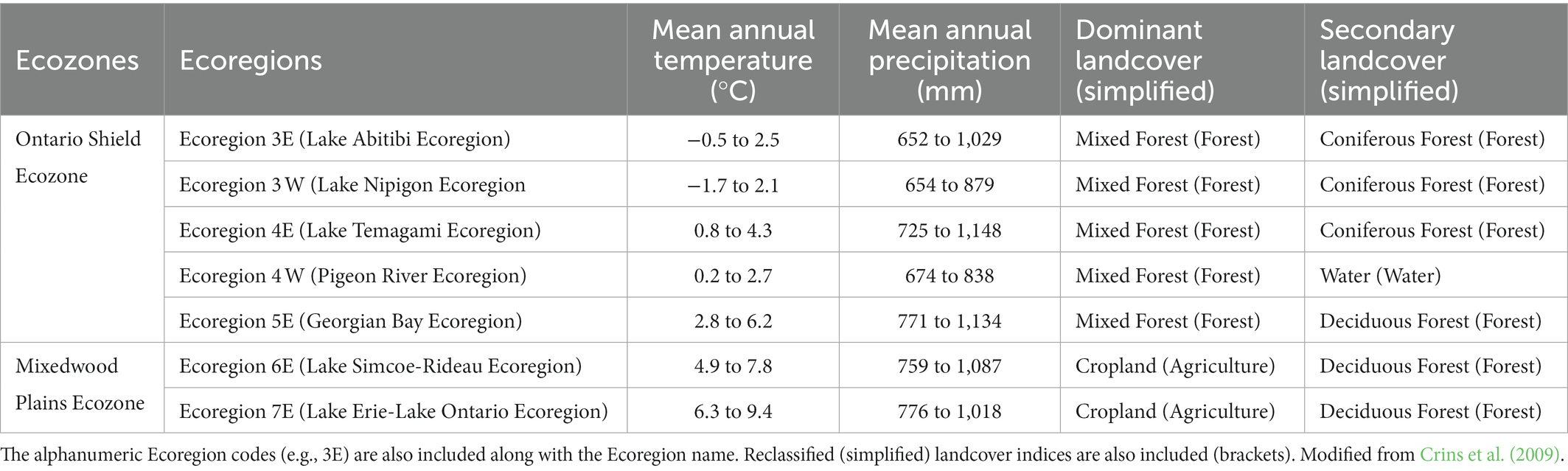
Table 1. Ecoregions within the Great Lakes Basin.
Terrestrially, urbanization is characterized by increased impermeable surfaces, high human populations, and alterations to natural environments (McKinney, 2002; Melles et al., 2003; Ferenc et al., 2014; Strohbach et al., 2019). In addition to changes to terrestrial landscapes, urbanization results in modifications to aquatic ecosystems (McDonald et al., 2013; Fritz et al., 2018). The likelihood of aquatic system modification is high, as most large population centers develop in areas that are close to large bodies of freshwater (Kummu et al., 2011; McDonald et al., 2013; Bosker and Buringh, 2017). In urban areas, freshwater streams tend to be modified from their natural states and can be characterized by channelized, straightened streams with increased flow variability, reduced riparian corridors, and higher percentages of impermeable surfaces in surrounding watersheds (McDonald et al., 2013; Fritz et al., 2018). Additionally, there is an increase in impervious cover (roads and concrete surfaces), buried natural channels, and the installation of storm drains that increase the speed at which stormwater reaches downstream channels (Brown et al., 2005). These stream modifications may improve longitudinal connectivity; but in turn, they decrease vertical and lateral connectivity (Brown et al., 2005).
The natural network patterns created by flowing water can be used to classify positions along the watersheds that they drain. Stream Strahler order classifications provide a well-known and easy to understand index of stream size and position in the watershed (Strahler, 1957; Hughes et al., 2011; Stenger-Kovács et al., 2014). Along the watershed, the conditions (natural or modified) created by a combination of flowing water and surrounding landcover impact the vegetation and by extension the organisms that live there (Nakano and Murakami, 2001; Allan, 2004). The zone of influence of streams extends beyond their surrounding areas through the provision of direct habitat (trees, shrubs, wetlands), the dispersal of organisms and the presence of resources and feeding opportunities several meters to hundreds of meters away (Bodie and Semlitsch, 2000; Baker et al., 2001; Figuerola and Green, 2002; Schofield et al., 2018; Recalde et al., 2020). Additionally, it should be noted that surrounding landscapes and riparian areas are distinctive in their hydrology and their impact on ecological structures (Naiman and Decamps, 1997; Baker et al., 2001; Wiens, 2002; Allan, 2004; Fritz et al., 2018). Recent research shows that network position along the stream also plays an important role in species diversity (Finn et al., 2011; Altermatt, 2013; Altermatt et al., 2013; Stenger-Kovács et al., 2014; Stearman et al., 2019). In keeping with an understanding that the intricate relationship between terrestrial and aquatic systems forms a complete landscape, watershed position in concert with landcover type, are expected to impact terrestrial species diversity metrics.
Despite the known importance of using a place-based approach in ecology, we are aware of no other ecological investigations that have examined bird species richness in relation to watershed position. We chose to use birds as our indicator species as they are generally well studied and thoroughly sampled. Landcover varies across the landscape, and it is understood that differences in landcover can impact avian species diversity metrics (Jones, 2001; Liu, 2022). Heterogenous landscapes are expected to provide greater benefits for species diversity than homogenous landscapes (Tews et al., 2004; Stein et al., 2014; Callaghan et al., 2019). For bird species, the availability of foraging and nest sites, prey availability, microhabitat conditions (shading, cooling, water), and predation rates all impact the selection of specific landcover classes (Jones, 2001; Chalfoun and Schmidt, 2012; Wilsey et al., 2017; Devries et al., 2018). The type of landcover that satisfies all requirements varies based on the species (Chalfoun and Schmidt, 2012). In addition, it is well-known that bird species composition and richness are often reduced in urban areas. Urbanization affects the composition and structure of natural bird species assemblages (Aronson et al., 2014; Ibáñez-Álamo et al., 2017; Sol et al., 2017). This reduction may be driven by the loss of evolutionarily distinct species (Sol et al., 2017) and the loss of species with more specialized functional roles (Sol et al., 2014; Concepción et al., 2015; Coetzee and Chown, 2016). Consequently, species in urban bird assemblages are expected to be less specialized, have higher levels of environmental tolerance (Bonier et al., 2007; Evans et al., 2011; Sol et al., 2014), and were initially expected to be closely related species (Sol et al., 2014). The idiosyncratic structure and landcover gradients of each urban area, however, impact species composition and species richness uniquely (Ferenc et al., 2014). More recent studies show that the effects of urbanization on species presence changes depending on the location of that urban area (Ferenc et al., 2014; Hensley et al., 2019). As a result, some studies demonstrate that urban areas have the potential to retain endemic native species and relatively high degrees of functional diversity (Müller et al., 2013; Aronson et al., 2014; Threlfall et al., 2016; Hagen et al., 2017): indeed, impacts of urbanization vary with location (Łopucki et al., 2013; Ferenc et al., 2014; Schütz and Schulze, 2015). The revelation of these location-based differences demonstrates the importance of conducting our research.
To adequately assess the effects of landcover and watershed position on terrestrial bird species richness, we used sample-based species accumulation curves. The theory behind these curves is based around the principle that increasing the number of points sampled increases the number of new species observed (Colwell and Coddington, 1994; Chiarucci et al., 2008). That is, the number of species that are observed is viewed as a function of the level of sampling effort (Colwell et al., 2004). Essentially these curves can provide an idea of the ecological structure of the areas sampled. Using SAC curves, it is possible to further understand and investigate the importance of landcover type and watershed position on species accrual.
Aligned with an understanding that terrestrial patches and aquatic systems are all part of the general landscape mosaic, and given the need to further understand the relationship between terrestrial species and aquatic systems, we examined the effects of aquatic system Strahler order (an index of watershed position), underlying landcover, and Ecoregion on terrestrial bird species richness patterns across the Ontario side of the Great Lakes Basin (GLB). We expect to observe a higher level of species richness in downstream areas as well as forested areas; however, some variation from this expectation is feasible due to underlying landcover and Ecoregion. Our primary objective for this work was to establish the climatic, hydrologic, and landcover features that are required to effectively “world build” while avoiding model over complication. We address the following related questions:
1. Given that urban areas are typically located in downstream areas, with richer soils and favorable climates, we expect to see urban areas retain a relatively high level of species in comparison to other landcover types while controlling for watershed position, and we pose the question: Does urban landcover retain a relatively high level of species richness in comparison to other landcover types evaluated in the GLB?
2. Does species richness, or more specifically, species accrual, change as we move toward downstream reach contributing areas while accounting for landcover classification and Ecoregion?
The Great Lakes Basin is characterized by a connected set of five lakes, with generally comparable climatic conditions (Scott and Huff, 1997; McDermid et al., 2015), and varied urban development conditions, creating the ideal region for applying and testing the idea that species richness accrual is faster in downstream watershed positions – even in urban watersheds. The Canadian side of the GLB, includes streams that drain into Lake Superior, Lake Huron, Lake Erie, and Lake Ontario (Figure 1). This study does not include streams or land areas from the United States side of the GLB because sampling efforts and methods differed across these states, and it was important to have consistent and comparable samples. The Great Lakes Basin hydrology layers were derived from the Great Lakes – St. Lawrence River Basin Watersheds (GLBW) package (Ontario Ministry of Natural Resources and Forestry – Provincial Mapping Unit, 2009). We further divide our study area into the Ecoregions that capture different portions of the GLB (Table 1). Human activities and development are influenced by the climatic conditions defined within Ecoregions. The northwest of Ontario is largely forested and has an historic forestry industry presence (Crins et al., 2009). The population density of this region is also relatively low resulting in lower incidences of urbanized landcover (Crins et al., 2009). To the southeast, where the climate is generally milder and the growing season is substantially longer, there is a high percentage of agriculture and urbanized landcover (Crins et al., 2009).
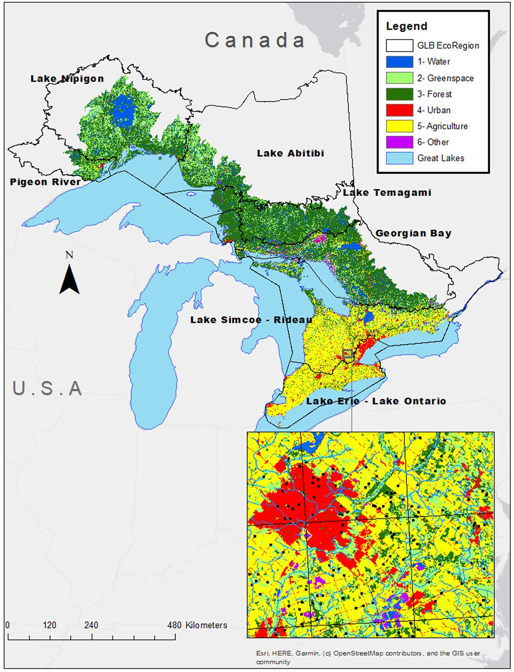
Figure 1. Map of study area (Canadian side of the Great Lakes Basin) showing landcover types and location of the Ecoregions. The inset map shows a few of the OBBA sampling locations. Pixel resolution is 15 m.
The Ontario Landcover Compilation Version 2 (OLCCv2) was used to define land cover classes in the GLB. The OLCCv2 is a combination of the following landcover packages: the Far North Landcover Version 1.4 (FNLCv1.4), the Southern Ontario Land Resource Information System, and The Provincial Landcover 2000 Edition (PLC2000) (Ontario Ministry of Natural Resources and Forestry, 2014). The OLCCv2 contained Landsat imagery for the entire Province of Ontario taken between the years 1999–2011: 1999–2002 (PLC2000), 1999–2002 (SOLRIS) and 2005–2011 (FNLCv1.4, Ontario Ministry of Natural Resources and Forestry, 2014). The standardized resolution of the OLCCv2 is fifteen (15) meters and the compilation uses the projection, NAD83 Lambert Conformal Conic (Ontario Ministry of Natural Resources and Forestry, 2014). The OLCCv2 contains twenty-nine (29) landcover classes, which are listed fully in Supplementary Table S1. The OLCCv2 was downloaded from Ontario GeoHub.1
Using the “reclassify” tool in ArcMap, the initial 29 landcover classes were condensed into six classes for the purpose of developing separate species accrual relationships by cover class. The six classes were: Urban, Greenspace, Agriculture, Forest, Water, and an additional class labeled Other (see Supplementary Table S1). “Urban” landcover defines built-up areas and their associated anthropogenic structures (Ministry of Natural Resources and Forestry Science and Research Branch, 2019). “Greenspace” typically includes all public green areas, including urban parks, wetlands, and recreational facilities (Hahs and McDonnell, 2006; Taylor and Hochuli, 2017; Suarez-Rubio and Krenn, 2018). We use the term “Greenspace” to represent natural landcover that did not fall into the definition of Forest (e.g., Hedgerows, Disturbance, Tallgrass Prairie, etc.): this landcover class included the most varied of the original OLCCv2 landcover classes. The “Agriculture” land class consisted of all agricultural areas including semi-natural areas (Ministry of Natural Resources and Forestry Science and Research Branch, 2019). “Forest” included all areas with tree cover greater than 60% (Lee et al., 1998). “Water” refers to water bodies such as lakes (Ministry of Natural Resources and Forestry Science and Research Branch, 2019), but for the purpose of this study streams were included implicitly by looking directly at the potential impact of watershed position. The “Other” category was used to classify any features that did not fall under any of the five categories (i.e., Bedrock, Sand, Gravel, and Cloud or Shadow, Supplementary Table S1).
In this study, “stream” refers to any size of river or flowing body of freshwater, and these are characterized using varying Strahler orders (Figure 2; Strahler, 1957). Ontario hydrology datasets and layers (within quaternary watersheds) were based on the Ontario Integrated Hydrology data (OIH; Provincial Mapping Unit, 2016). Stream orders were grouped to ensure adequate bird point count sample sizes in downstream areas as there are more headwater areas than mid-order and downstream ones. Watershed positions (WSP) were attributed using the Strahler order classification of stream reaches as follows:
• Headwaters WSP (HW) include first (1st) and second (2nd) order (Meyer et al., 2007; Finn et al., 2011)
• Midwaters WSP (MW) are third (3rd) and fourth (4th) order streams (Finn et al., 2011)
• Downstream / outlet (OUT) WSP are greater than or equal to (≥) fifth (5th) order streams (Finn et al., 2011).
Figure 2. Schematic demonstrating how both Strahler stream order and land cover categories were used to characterize bird sampling locations. Key: Urban – Red, Greenspace – Green, Agricultural – Yellow.
First and second-order streams that drained directly into the Great Lakes were removed. Their exclusion was necessary to ensure that these smaller stream areas do not skew the results due to lake effects, as they would be classified as headwaters by the study criteria, but they are located, and possibly behaving like, downstream WSPs given their position relative to the Great Lakes.
All GIS processing was completed using ArcMap 10.7.1. Using the “Clip” tool in ArcMap, the enhanced stream flow layer from the OIH was cropped to the extent of the GLB study area. Streamflow lines were then “Dissolved” so the only identifying information was Strahler order. This simplification allowed for the compilation of numerous enhanced flow datasets to be compared. The “Multiplepart to Singlepart” feature was then applied to separate streams of similar orders into independent features allowing for the selection of these streams individually. All separate enhanced flow layers were then combined using the “Merge” feature. The merged enhanced flow of the GLB was then used to select the boundaries located on the shore of the Great Lakes. Headwater streams that flow directly into the lakes were then spatially selected and removed from analysis.
Point count data were obtained from the Ontario Breeding Bird Atlas (OBBA) 2001–2005. This was the second such Atlas compiled for the Province of Ontario. The first OBBA covered 1981–1985 and the upcoming 3rd OBBA surveys began in 2021. The OBBA dataset contains species observations expected to represent most breeding birds within Ontario. Sampling counts occurred between May and July (dates varied depending on location) of the years 2001 through 2005 (Bird Studies Canada, Environment Canada’s Canadian Wildlife Service, Ontario Nature, Ontario Field Ornithologists and Ontario Ministry of Natural Resources, 2008). Surveys for the OBBA were conducted within 10 × 10 km squares covering the province (Bird Studies Canada, Environment Canada’s Canadian Wildlife Service, Ontario Nature, Ontario Field Ornithologists and Ontario Ministry of Natural Resources, 2008). This covered the regions within the Great Lakes Basin Watershed. Each point count was observed for 5 min and all bird species within a 100 m radius were recorded by birders able to identify birds by their song (Bird Studies Canada, Environment Canada’s Canadian Wildlife Service, Ontario Nature, Ontario Field Ornithologists and Ontario Ministry of Natural Resources, 2008). A minimum of twenty-five (25) of these observations were completed per square by volunteer birders (for the majority of the OBBA) to ensure that the abundance of each species was well represented, but a minimum of 10-point counts per square was accepted in the final year (Cadman et al., 2007). Finally, all observations were validated by professional ornithologists and Regional Coordinators of the OBBA sampling team (Bird Studies Canada, Environment Canada’s Canadian Wildlife Service, Ontario Nature, Ontario Field Ornithologists and Ontario Ministry of Natural Resources, 2008).
The OBBA dataset including rare species was retrieved via a data request to the Nature Counts portal. The dataset was then modified and cleaned in R version 4.0.3 (R Core Team, 2020) before being assessed further in ArcMap. Point counts were initially located by latitude and longitude, which were then transformed and projected to NAD 1983 Ontario Lambert Conformal Conic. For this study, we selected point counts that were located within the limits of the GLB. This was completed using the “Clip” tool in ArcMap. In some instances, a particular point was sampled on multiple occasions; for these instances, the sample with the highest total species richness was selected to represent that point count.
We used the observation distance radius, i.e., 100 m to characterize the underlying landcover around point count sampling locations. The majority landcover (LCMAJ) of each of these buffers was then calculated using the “zonal statistics” tool in ArcMap. This provided a more accurate landcover description of the surveyed area than that of the underlying landcover values at the exact point count location. The distance of each buffer to the nearest stream was also included using the “near” tool. This feature was used to identify the Strahler order associated with that sample point.
Upon completion of our spatial analysis, each point count contained information on the following:
• Species incidence and abundance.
• Majority landcover type at 15 m resolution.
• Nearest Strahler Order.
• WSP Classification (i.e., headwaters, midwaters, and downstream).
• Ecoregion.
Point count data were divided into subsets based on Ecoregion-Landcover Classification-Watershed position (ER-LCC-WSP) using the “subset” function in R. From here on we will refer to these subsets as subgroups. The number of sites in each subgroup was evaluated using the “BiodiversityR” package and the function “diversitycomp,” which provided a count of sites at each subgrouping (Kindt and Coe, 2005). The number of sites located in the OUT WSP in each subgroup had the smallest number of sites per subgroup category. The smallest number was then used as the number of samples to create our Species Accumulation Curves (SACs). Through this method, we assessed each WSP in a specific subgrouping as evenly as possible to glean a better understanding of the impact of watershed position. Additionally, species diversity metrics including richness, abundance, Shannon, and Simpson were calculated for each subgroup.
The first steps in creating the SACs involved using the “vegan” package function: specaccum (Oksanen et al., 2020). The “exact” method, which provides the expected mean richness for a specified number of sampling sites, was used (Kindt and Coe, 2005). Using both AIC and BIC to test model fit, the Lomolino model outperformed other SAC models (i.e., Gleason, Gitay, and Arrhenius) in most of the curves created. The resultant parameters of Lomolino fitted SACs are in the form of a slope, an asymptote, and an xmid. Slopes of the Lomolino models represents the slope at the inflection point, or the point on the slope where the concavity of the curve changes (Lomolino, 2001). In terms of the Lomolino model, this inflection point also represents the maximum rate of increase in species richness (Lomolino, 2001). Fitted slope is therefore the parameter that allows for estimating the rate of species accrual at its greatest point. The asymptote represents the maximum richness of the sites sampled (Lomolino, 2001). The xmid is the number of points at which half the total species richness is achieved, this parameter however was not included for further analysis.
Upper and lower confidence intervals around these Lomolino model parameters (slopes and asymptotes) were then used to create a range of possible curves and sampled 1,000 times. From these repeated samples, we extracted the curve coefficients, i.e., slopes and asymptotes as the response variable in our statistical models, but accrual asymptotes greater than the observed 216 species (total species count) were removed. The 1,000 SAC iterations increased the likelihood of covering the full range of sampling possibilities from the existing community.
Using mixed effect models (MEM), we evaluated the relationship between our response variables, i.e., slope and asymptote, respectively, and the predictor variables, i.e., landcover class (LCC), watershed position (WSP), and Ecoregion in which the points making up the SACs were located. Species accrual slopes or asymptotes were in the form of positive nonzero numbers, therefore the Gamma distribution with a log link was used (Bolker et al., 2009; Harrison et al., 2018). The use of a mixed model approach allowed us to estimate the fixed effects of land cover class (LCC) and watershed position (WSP) on our response variables while controlling for Ecoregion as a random effect influencing both slopes and intercepts (see GLMM section below) allowing us to characterize random variation caused by the geographical Ecoregion of sample sites. Several models were tested and compared based on their AIC using the “anova” function. The most parsimonious models that did not include confounded variables were included.
Generalized linear mixed models were fit using the Gamma family with a log link and estimated using maximum likelihood (ML) and the BOBYQA optimizer. Use of a log link produced log transformed estimates. Two separate models were included, (1) slope as the response variable and (2) asymptote as the response variable. To predict our response variables, LCC and WSP were included as fixed effects with interactions, and Ecoregion was included as a random effect impacting parameter slopes and intercepts.
Additionally, we employed the use of Generalized Additive Models to further assess non-linearities in the relationship between our response variables and predictors as they vary by Ecoregion. Predictor variables were converted to a logit binary classification with Forest = 1, Greenspace = 2, Agricultural = 3, and Urban = 4. This was also done with WSP where HW = 1, MW = 2 and OUT = 3. All analyses were completed in R version 4.0.3 (R Core Team, 2020) using the mgcv package (Wood, 2011).
Across the sites included in this study, a total of 216 species of birds were observed. This total richness represents approximately 80% of the roughly 270 confirmed breeding species of Ontario (Cadman et al., 2007). A total of 34,936-point count stations were included in our analysis. Ecoregion sampling varied with Lake Simcoe-Rideau being the most sampled region while Pigeon River was under sampled resulting in its exclusion from further analysis. The highest richness was observed in the Lake Simcoe-Rideau Agricultural landcover, the highest Shannon diversity was observed in Georgian Bay Greenspace landcover class, and the highest inverse Simpson was calculated in Georgian Bay Agricultural landcover (Supplementary Table S2). The values of these diversity indices are likely impacted by the levels of sampling, further supporting our decision to use SACs to equalize efforts among watershed position.
Across the Great Lakes Basin Watershed, slopes ranged from 1.47 to 3.14 whereas asymptotes ranged from 66.30 to 215.50 (Supplementary Tables S3, S4). The highest mean slope (2.30) was found in the Lake Abitibi – Forest – MW subgroup with the highest mean asymptote (162.47) found in the Georgian Bay – Forest – MW subgroup (Supplementary Tables S3, S4). The slope and asymptote parameters from the SACs are presented in boxplots (Figures 3, 4). Boxplots show variation in the rates of accrual due to a combination of landcover type, watershed position, and Ecoregion in which the points were found. Outliers were found at both the upper and lower ranges of the slope parameter with more outliers located at the upper range. In the asymptote data, outliers were only located at the upper range of the boxplots. This issue was addressed by iterating these curves 1,000 times and removing all asymptotes greater than 216 which was the total species count in this study from further analysis. The likelihood of overestimation rather than underestimation is a function of the species accrual methodology whereby it is not possible for the number of species to decrease with increasing sample size. With slopes, this is not the case. That is, it was possible to have a high slope in one iteration of the curve followed by a lower slope in another. A summary of slopes and asymptotes from the complete set of SACs can be found in supplementary tables and figures (Supplementary Tables S3, S4).
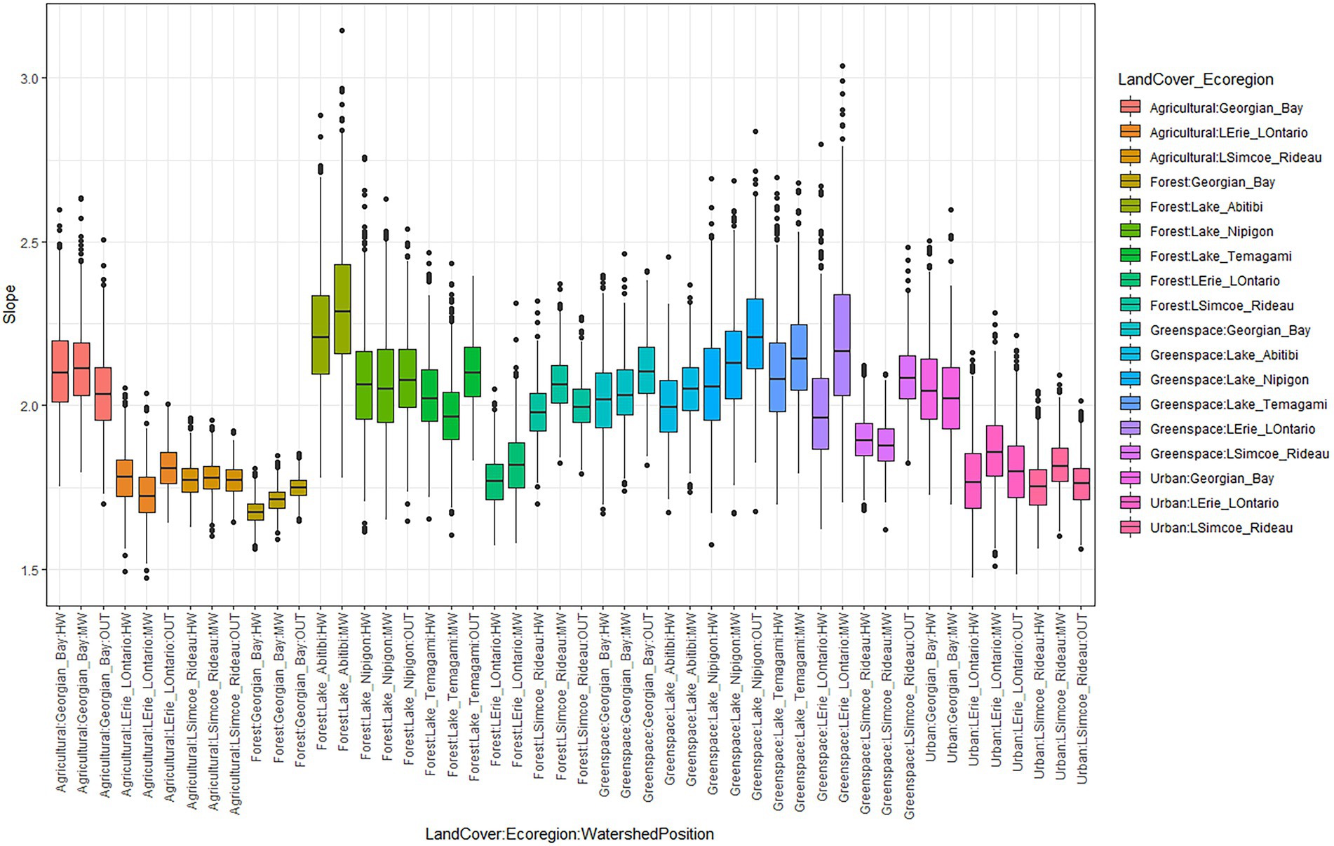
Figure 3. Boxplots showing the effect of Ecoregion, land cover type and watershed position on slope.
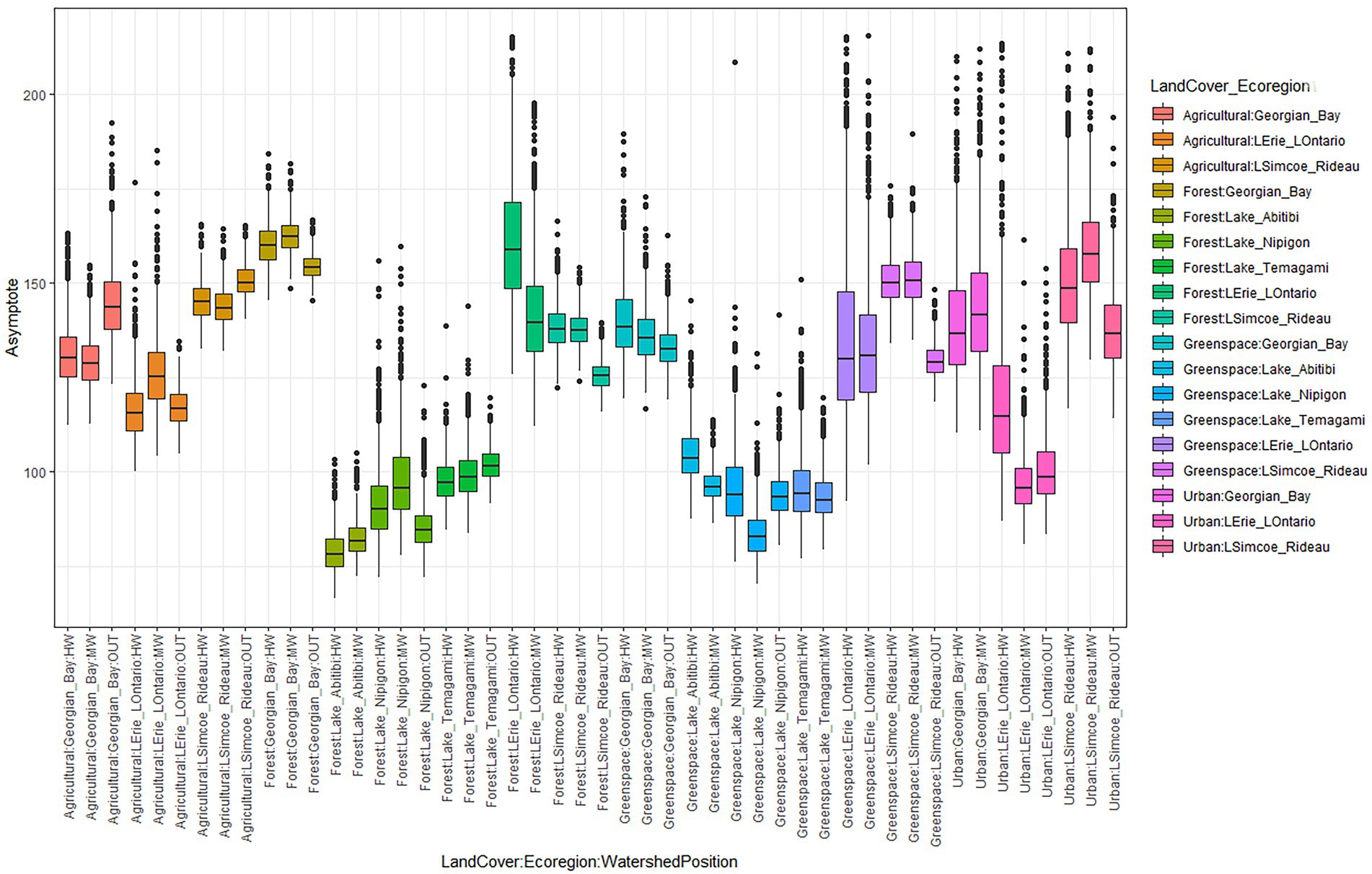
Figure 4. Boxplots showing the effect of Ecoregion, land cover type, and watershed position on asymptote.
To gain a better understanding of the relationship between the asymptotes and slopes of our species accrual curves, we created scatter plots for each subgroup to examine these variables in concert. There was an inverse curvilinear relationship between slopes and their corresponding asymptotes such that steeper slopes corresponded with lower asymptotes (Figure 5). This inverse relationship was not entirely surprising given that with less heterogeneity in an LCC, species accrual is expected to be faster and corresponding asymptotes lower; whereas increased heterogeneity in an LCC should result in more unique species observed as sampled points increase, leading to a slower rate of accrual and higher asymptotes (Thompson and Withers, 2003). When accounting for watershed position, this relationship varied further with the Ecoregion – landcover combinations. Looking at Figure 5, we can see that even at the same slope, many HW, MW, and OUT accrual curves differed in their corresponding asymptote. This provides evidence that watershed position plays a role in the rate of species accrual.
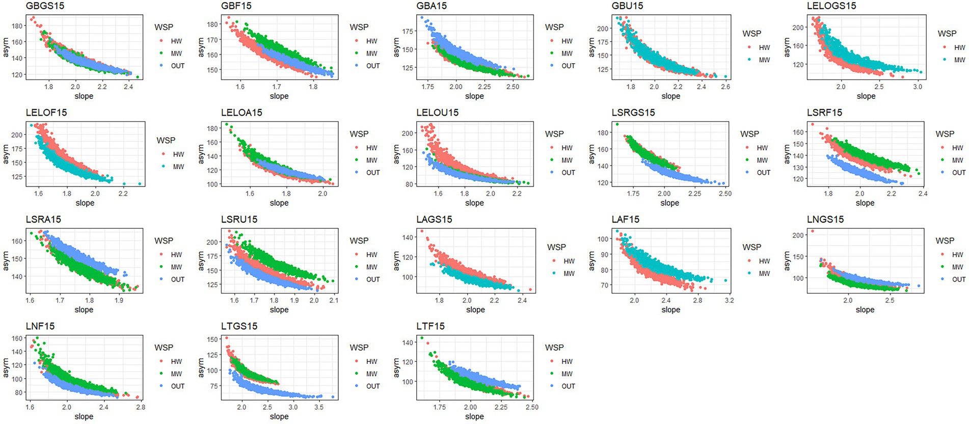
Figure 5. Scatterplots showing the relationship between slopes and asymptotes within each subgroup. Key: -Ecoregion: GB- Georgian Bay, LELO- Lake Erie Lake Ontario, LSR - Lake Simcoe Rideau, LN - Lake Nipigon LA- Lake Abitibi, LT - Temagami. Landcover: F- Forest, A- Agricultural, GS- Greenspace, U- Urban.
Rates of species accrual were estimated using the model formula: slope ~ LCC ✳ WSP + (1 + LCC | Ecoregion) + (1 +WSP | Ecoregion). The model’s explanatory power related to the fixed effects alone was substantial (marginal R2 = 0.69). The model’s intercept, corresponding to LCC = Forest and WSP = HW, was 0.67 (95% CI [0.66, 0.68], p < 0.001). Greenspace had the highest estimates among LCC whereas OUT had the highest parameter estimates for WSP (Table 2).
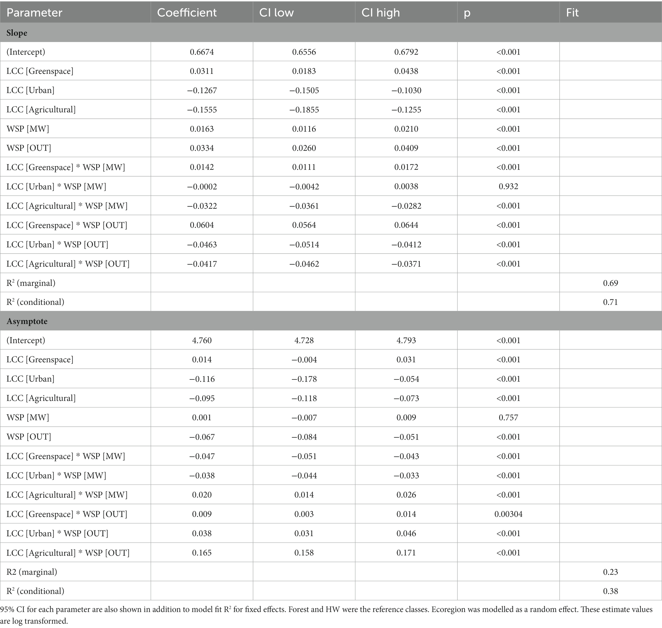
Table 2. Results of GLMMs for slope and asymptote.
Maximum species richness was estimated using the model formula: asymptote ~ LCC ✳ WSP +(1 + LCC | Ecoregion) + (1 +WSP | Ecoregion). The model’s total explanatory power was fair (conditional R2 = 0.38) and the part related to fixed effects alone was 0.23 (marginal R2). The model’s intercept, corresponding to LCC = Forest and WSP = HW, was at 4.76 (95% CI [4.73, 4.79], p < 0.001. The highest mean asymptote estimates were for Greenspace and MW, respectively (Table 2).
The explanatory power of our GLMMs for asymptotes were not as strong as models for slope. To further explore our data and determine how relatively robust these results were when a different model structure was used, we fit generalized additive models (GAMs) to each of our response variables.
Generalized additive models were also fit using the Gamma family with a log link (estimated using REML and outer optimizer) to predict slope and asymptote, respectively, with Ecoregion, LCC, and WSP.
Model formula: slope ~ Ecoregion + s(LCC, k = 4, by = Ecoregion) + s(WSP, k = 3, by = Ecoregion)). The model’s explanatory power can be considered substantial (R2 = 0.61). This model explained 63.4% of the deviance. The model’s intercept, corresponding to Ecoregion = Georgian Bay was at 0.66 (p < 0.001). Lake Temagami had the greatest effect (0.776) on slope while Lake Erie – Lake Ontario (0.633) had the smallest effect (Table 3 and Figures 6A,B).
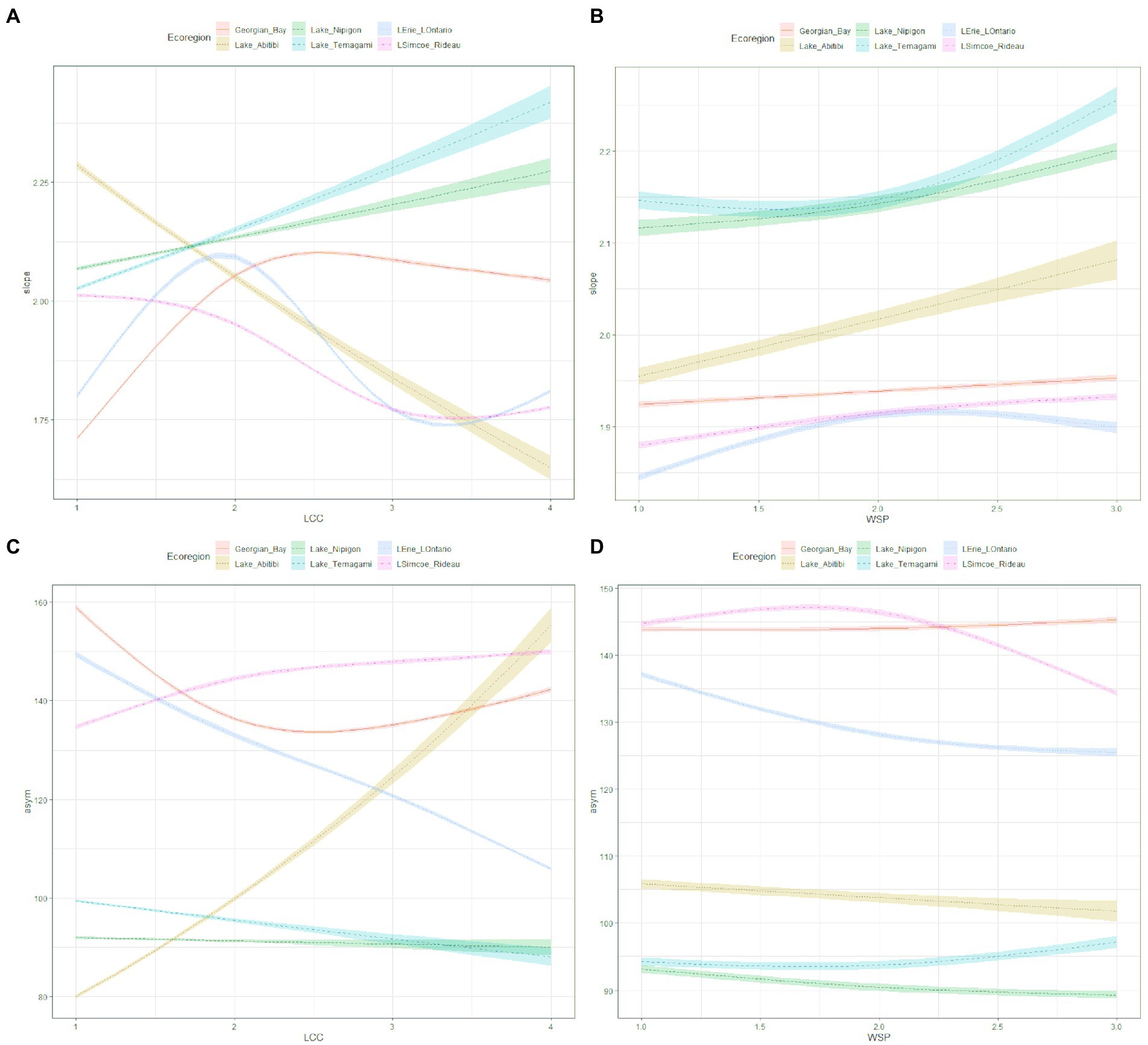
Figure 6. Results of GAM showing: (A) the slope in relation to Ecoregion and landcover class interacting; (B) the slope in relation to Ecoregion and watershed position interacting; (C) asymptote in relation to the interaction between Ecoregion and landcover class; (D) asymptote in relation to the interaction between Ecoregion and watershed position. Predictor variables were converted to a logit binary classification with Forest = 1, Greenspace = 2, Agricultural = 3, and Urban = 4. This was also done with WSP where HW = 1, MW = 2 and OUT = 3.

Table 3. Results of GAMs showing the ecoregion estimates and 95% CI for both slope and asymptote.
Model formula: asymptote ~ Ecoregion + s(LCC, k = 4, by = Ecoregion) + s(WSP, k =3, by = Ecoregion)). The model’s explanatory power was substantial at R2 = 0.82. This model explained 84.4% of the deviance. The model’s intercept was at 4.97 (p < 0.001), which corresponds to Ecoregion = Georgian Bay. Georgian Bay had the greatest effect (4.972) on the asymptote parameter with Lake Nipigon exhibiting the lowest effect (4.513) (Table 3 and Figures 6C,D).
Bird species diversity and abundance in the Great Lakes Basin is high relative to other parts of Ontario and Canada, providing an ideal watershed mosaic for this study since we were able to sample several landcover types located along different watershed positions all nested within a variety of Ecoregions. The presence of several landcover types, as well as the presence of streams in these regions, supports a variety of organisms (Spackman and Hughes, 1995; Baker et al., 2001). Many bird species were sampled in our analysis (216 in total), representing species across multiple trophic levels and occupying a wide variety of niches. Using Ontario Breeding Bird Atlas data, we created SACs and used these to study the rate of species accrual and potential maximum species richness in relation to watershed position, landcover type, and Ecoregion. When isolating the effects of land cover type, we found that on average, across the GLB, Forest landcover exhibited a lower mean species accrual rate (slope) than Greenspace (Table 2). Similarly with the asymptotes, Forest was again outperformed by Greenspace (Table 2). In thinking about Greenspace as public green areas, this pattern was unexpected and contradicted our initial expectations; however, given the way we defined Greenspace to include a heterogeneous mixture of landcover classes (e.g., Marsh, Hedgerows, Disturbance, Tallgrass Prairie) it is perhaps not surprising that this cover class exhibited a greater mean rate of species accrual (Turner and Tjørve, 2005; Kallimanis et al., 2008; Stein et al., 2014). Urban landcover within some subgroups exhibited species accrual rates and maximum richness estimates that were not only comparable to, but sometimes greater than, other subgroups (Supplementary Tables S3, S4).
Watershed position also matters to the rates of species accrual and potential maximum species richness (asymptotes). When looking at each subgroup (i.e., same Ecoregion and landcover conditions), we see that there was variation in species accrual rates within a given subgroup due to differences in WSPs (Figure 3). The climatic conditions described by Ecoregion further modulates the effects of both land cover and WSP for species accrual and maximum richness (Supplementary Table S3). LCC-WSP subgroups located within different Ecoregions showed varying effects on species accrual rates, estimated maximum species richness, and other species diversity metrics (Supplementary Table S2).
The rate of species accrual tells the observer how rapidly a system increases in species with each additional point sampled (Colwell and Coddington, 1994; Chiarucci et al., 2008). Here, the rate of accrual provides an idea of the relative favourability of underlying habitat conditions, measured as the combination of Ecoregion, landcover type, and watershed position. One perspective about the information derived from a steep slope is that it is a system level metric where a smaller sample is required to reveal most of that system’s species richness (Thompson and Withers, 2003; Dove and Cribb, 2006). Alternatively, curves with shallower slopes, i.e., a slower rate of accrual, require a larger number of samples to achieve a similar level of richness (Thompson and Withers, 2003; Dove and Cribb, 2006). Although, not necessarily equal to a high level of richness, high rates of accrual may be favorable to a highly functional ecosystem particularly in remnant landscapes (Flather, 1996). Additional work is needed to further explore this idea.
Ecoregions are defined based on their climatic conditions, historical landcover, as well as surface water presence, all having the potential to affect the types of species present in that area (Crins et al., 2009; Yang et al., 2011). Based on our results, estimates for Lake Abitibi, Lake Nipigon, and Lake Temagami, which are located to the Northwest of the GLB showed faster rates of species accrual than Georgian Bay, Lake Erie – Lake Ontario and Lake Simcoe – Rideau, located in the more southern parts of the GLB (Figure 1 and Table 3). These patterns however were modified when looking at our subgroups in their entirety (Supplementary Tables S3 and Figure 3). Independently, our GAM results show that Lake Temagami had the highest parameter estimate for slope, and Georgian Bay exhibited the highest asymptote estimate (Table 3). Climatic variability in these Ecoregions (Table 1) plays a role in affecting rates of species accrual (Figure 3, Kallimanis et al., 2008). The Ecoregions of Lake Nipigon, Lake Abitibi, and Lake Temagami are all described as having cooler mean temperatures and shorter summers than Georgian Bay, Lake Erie - Lake Ontario and Lake Simcoe – Rideau. Historical land use patterns also varied among Ecoregions with higher levels of agriculture to the south and maintained forests to the northwest of the GLB (Crins et al., 2009; Figure 1). As expected, regional context and climatic conditions were captured by the Ecoregional (random) effects in our models. Surprisingly, Agriculture and Urban landcovers in Georgian Bay had the steepest slopes detected (after mostly northern forests) indicating relative uniformity in these landcover types because a smaller sample would be required to reveal most of the system’s richness. This result further highlights the effect of Ecoregion on species accrual rates. However, the same was not true for Agricultural and Urban landcover in southern regions (Simcoe, Erie-Ontario) where slopes were shallow indicating the need for more samples to determine maximum richness. Shallower slopes in more human managed landcover types are in keeping with the results of other studies (Flather, 1996). Several of these combinations showed that these factors further compound to affect the rates of accrual seen at a specific watershed position (Figure 3).
Our first research question focused on observing the ability of urban landscapes to retain a relative amount of species richness and rates of accrual. The ability of urban environments to maintain and attract ecological richness is of the utmost importance to the future of our cities. Our results show that urban environments have the potential to maintain a relatively high species richness that varies with watershed position (Figure 4). Several studies speak to the variability of species diversity patterns observed within urban settings (Ferenc et al., 2014; Hensley et al., 2019). This pattern is further enhanced when looking at urban areas in the context of the Ecoregions in which they are embedded. In our study, Ecoregions that were historically more urbanized, i.e., Lake Erie – Lake Ontario and Lake Simcoe – Rideau, have the potential to maintain species diversity (Figures 1, 4). Particularly for the Lake Simcoe – Rideau Ecoregion, Urban landcover classes at mid watershed positions exhibited a mean asymptote (159.32 – MW) and maximum species richness (138) that were among the highest overall (Figure 1; Supplementary Tables S2, S4). Much of the surrounding landcover associated with the urban environment in these regions is classified as agricultural, which in previous studies is noted to modify the species that occur within these landscapes (Sirami et al., 2019; Lee et al., 2022). In fact, Lake Erie – Lake Ontario and Lake Simcoe – Rideau are both described as having cropland (Agricultural) as their primary landcover type (Crins et al., 2009). This heterogeneous combination of landcover under the more southern climatic conditions of the Mixed Wood Plain Ecozone may provide ideal conditions for maintaining relatively high species richness (Figure 1 and Supplementary Table S2).
Greenspace estimates outperformed Forest in terms of rates of accrual and asymptotes (Table 2). Though this was unexpected, it may be explained by several factors. Our classification of Greenspace is comprised of different (12) landcover types that were characterized by some unique open spaces (e.g., Tallgrass Prairie, Swamp, and Marsh). Landcover heterogeneity is understood to influence species diversity metrics, and several of the landcover types included in our Greenspace index were found within our study area only in small amounts. All landcover types included in the Greenspace class are characterized by possessing <60% tree cover and our grouping was done to ensure sufficient bird sampling points were captured. Whereas the Forest cover class was less heterogeneous (Supplementary Table S1). Our Forest class is comprised mainly of coniferous, deciduous, and mixed forest. The variability of the cover classes included in Greenspace likely provides habitats that are favorable to a greater number of avian species than the habitat provided by the Forest landcover class due to the greater heterogeneity of the types included in the Greenspace class (Turner and Tjørve, 2005; Kallimanis et al., 2008; Stein et al., 2014).
We hypothesized that species accrual rates would be higher as you move toward downstream positions. From our results, when looking solely at the effect of watershed position, we see that MW and OUT exhibit estimates that are higher than those of HW (Table 2). However, in the context of our subgroups, the impact of watershed position was highly variable in relation to Ecoregion and the landcover types that these streams flowed through (Figure 3 and Figure 4). Indeed, like riparian areas, the ecological function and impact of all watershed positions is not the same (Baker et al., 2001; Thorp et al., 2006). The variability of SAC slopes and asymptote estimates with WSP are in-line with other papers that emphasize the effects of the variability of stream reaches and the additional impact of their surrounding landscape (Baker et al., 2001; Wiens, 2002; Yang et al., 2011; Soininen et al., 2015). Our results show that landcover type is further modified by watershed position in its effect on species diversity metrics. As our approach is based on observed patterns and statistical relationships, we cannot directly deduce causality; nor can we extract the exact mechanisms that cause these differences. However, there is an extensive literature that can be used to explore the mechanisms of WSP on species. The impact of watershed position can be explained best by understanding the potential effect of stream size on aquatic species accrual rates (Minshall et al., 1985). It can be hypothesized that the patterns that increase discharge and in-turn species richness, may also translate to impacts on neighboring terrestrial areas. In addition to the size of the streams, the structure of riparian areas and the impact that they have on the surrounding landscape also changes with a change in watershed position (Baker et al., 2001; Wiens, 2002; Allan, 2004). This relationship changes when looking at mean asymptotes with MW exhibiting the greatest impact on maximum richness (Table 2). Streams may also flow through several Ecoregions from headwater to outlet (longitudinal) resulting in further differences in hydrology, geomorphic features such as soil and climatic conditions including precipitation (Yang et al., 2011). There may also be differences in subsidies from freshwaters systems to the surrounding landscape at different locations along the stream (Lamberti et al., 2020). The variability of watershed position and its impact on species accrual rates remained throughout our study.
We face limitations however as we did not investigate SACs within specific watersheds, so we cannot speak to the impact of sampling the same watershed in different positions. This limitation was overcome partially by our use of randomizations within the 95% CIs of each slope or asymptote. We are confident that we captured the full range of variability in SACs across LCC and WSPs without explicitly accounting for within watershed effects.
The landscape mosaic of the Great Lakes Basin is highly variable, and this variability is reflected in the results that were obtained. Across Ecoregions, the effects of landcover and watershed position vary in their impact on several species’ diversity metrics. We conclude that although our models showed Greenspace and river outlet catchments had the greatest mean effect on the rate of species accrual across the GLB, accrual rates were influenced by interactions between, Ecoregion, landcover type, and watershed position. There was an inverse relationship between accrual rates and maximum species richness such that maximum species richness varied considerably with equivalent accrual rates. As ecologists work to develop worldview models that adequately capture the importance of regional context, and as they adopt a watershed position-based approach, our results showed that consideration needs to be paid to the inclusion of interactions between region context, landcover, and position in the watershed, particularly when considering the impacts of urban and agricultural development.
Future studies will explore the impact of surrounding landcover type on the patterns observed through the application of pixel sizes of increasing magnitude. The goal will be to approximate how birds use the landscape at a variety of spatial scales. To further explore the requirements for “world building,” additional work will be required to understand the impact of scales and local dimensionality (height of trees, depth of streams, etc.) on rates of species accrual and richness. Recommended research could also include an exploration of how species guilds or functional groups vary by Ecoregion, landcover class, and watershed position.
The datasets presented in this study can be found in online repositories. The names of the repository/repositories and accession number(s) can be found at: https://doi.org/10.32920/ryerson.21187699.v1.
AJ and SM worked on conceptualization, creation of methodology, validation, and data analysis. AJ was responsible for data acquisition, analysis, interpretation, original draft preparation, and visualization. SM provided funding acquisition, supervision, reviews, and editing of manuscript. All authors have agreed to be accountable for all aspects of the work, read, and agreed to the published version of the manuscript.
We gratefully acknowledge a Toronto Metropolitan University (TMU) Black Graduate Student Scholarship and several TMU Graduate Scholarships to AJ. The research was also supported by a Natural Sciences and Engineering Research Council of Canada grant to SM (DG 03834–2015).
Thanks to the official sponsors of the Ontario Breeding Bird Atlas (Bird Studies Canada, Canadian Wildlife Service, Federation of Ontario Naturalists, Ontario Field Ornithologists, and Ontario Ministry of Natural Resources) for supplying Atlas data, and to the thousands of volunteer participants who gathered data for the project.
The authors declare that the research was conducted in the absence of any commercial or financial relationships that could be construed as a potential conflict of interest.
All claims expressed in this article are solely those of the authors and do not necessarily represent those of their affiliated organizations, or those of the publisher, the editors and the reviewers. Any product that may be evaluated in this article, or claim that may be made by its manufacturer, is not guaranteed or endorsed by the publisher.
The Supplementary material for this article can be found online at: https://www.frontiersin.org/articles/10.3389/fevo.2023.1081230/full#supplementary-material
Allan, J. D. (2004). Landscapes and riverscapes: the influence of land use on stream ecosystems. Annu. Rev. Ecol. Evol. Syst. 35, 257–284. doi: 10.1146/annurev.ecolsys.35.120202.110122
Altermatt, F. (2013). Diversity in riverine metacommunities: a network perspective. Aquat. Ecol. 47, 365–377. doi: 10.1007/s10452-013-9450-3
Altermatt, F., Seymour, M., and Martinez, N. (2013). River network properties shape α-diversity and community similarity patterns of aquatic insect communities across major drainage basins. J. Biogeogr. 40, 2249–2260. doi: 10.1111/jbi.12178
Aronson, M. F., La Sorte, F. A., Nilon, C. H., Katti, M., Goddard, M. A., Lepczyk, C. A., et al. (2014). A global analysis of the impacts of urbanization on bird and plant diversity reveals key anthropogenic drivers. Proc. R. Soc. Lond. Ser. B 281:20133330. doi: 10.1098/rspb.2013.3330
Baker, M. E., Wiley, M. J., and Seelbach, P. W. (2001). GIS-based hydrologic modeling of riparian areas: implications for stream water quality. J. Am. Water Resour. Assoc. 37, 1615–1628. doi: 10.1111/j.1752-1688.2001.tb03664.x
Bartrons, M., Sardans, J., Hoekman, D., and Peñuelas, J. (2018). Trophic transfer from aquatic to terrestrial ecosystems: a test of the biogeochemical niche hypothesis. Ecosphere 9:e02338. doi: 10.1002/ecs2.2338
Bilby, R. E. (1988). “Interactions of aquatic and terrestrial systems” in Streamside Management: Riparian Wildlife and Forestry Interactions. College of Forest Resources No. 59. ed. K. J. Raedeke (Seattle, WA: University of Washington), 13–29.
Bird Studies Canada, Environment Canada’s Canadian Wildlife Service, Ontario Nature, Ontario Field Ornithologists and Ontario Ministry of Natural Resources (2008). Ontario breeding bird atlas database. Available at: https://www.birdsontario.org/jsp/downloaddata.jsp (accessed June 9, 2020)
Böck, K., Polt, R., and Schülting, L. (2018). “Ecosystem Services in River Landscapes” in Riverine Ecosystem Management. Aquatic Ecology Series. eds. S. Schmutz and J. Sendzimir, vol. 8 (Cham: Springer), 413–433.
Bodie, J. R., and Semlitsch, R. D. (2000). Spatial and temporal use of floodplain habitats by lentic and lotic species of aquatic turtles. Oecologia 122, 138–146. doi: 10.1007/PL00008830
Bolker, B. M., Brooks, M. E., Clark, C. J., Geange, S. W., Poulsen, J. R., Stevens, M. H. H., et al. (2009). Generalized linear mixed models: a practical guide for ecology and evolution. Trends Ecol. Evol. 24, 127–135. doi: 10.1016/j.tree.2008.10.008
Bonier, F., Martin, P. R., and Wingfield, J. C. (2007). Urban birds have broader environmental tolerance. Biol. Lett. 3, 670–673. doi: 10.1098/rsbl.2007.0349
Bosker, M., and Buringh, E. (2017). City seeds: geography and the origins of the European city system. J. Urban Econ. 98, 139–157. doi: 10.1016/j.jue.2015.09.003
Brown, L. R., Gray, R. H., Hughes, R. M., and Meador, M. R. (2005). Introduction to effects of urbanization on stream ecosystems. Am. Fish. Soc. Symp. 47, 1–8.
Cadman, M. D., Sutherland, D. A., Beck, G. G., Lepage, D., and Couturier, A. R. (2007). Atlas of the Breeding Birds of Ontario, 2001–2005. Bird Studies Canada, Environment Canada, Ontario Field Ornithologists, Ontario Ministry of Natural Resources, and Ontario Nature: Toronto, 706
Callaghan, C. T., Bino, G., Major, R. E., Martin, J. M., Lyons, M. B., and Kingsford, R. T. (2019). Heterogeneous urban green areas are bird diversity hotspots: insights using continental-scale citizen science data. Landsc. Ecol. 34, 1231–1246. doi: 10.1007/s10980-019-00851-6
Chalfoun, A. D., and Schmidt, K. A. (2012). Adaptive breeding-habitat selection: is it for the birds? Auk 129, 589–599. doi: 10.1525/auk.2012.129.4.589
Chase, J. M. (2000). Are there real differences among aquatic and terrestrial food webs? Trends Ecol. Evol. 15, 408–412. doi: 10.1016/S0169-5347(00)01942-X
Chiarucci, A., Bacaro, G., Rocchini, D., and Fattorini, L. (2008). Discovering and rediscovering the sample-based rarefaction formula in the ecological literature. Community Ecol. 9, 121–123. doi: 10.1556/ComEc.9.2008.1.14
Coetzee, B. W. T., and Chown, S. L. (2016). Land-use change promotes avian diversity at the expense of species with unique traits. Ecol. Evol. 6, 7610–7622. doi: 10.1002/ece3.2389
Colwell, R. K., and Coddington, J. A. (1994). Estimating terrestrial biodiversity through extrapolation. Philos. Trans. R. Soc. Lond. Ser. B 345, 101–118. doi: 10.1098/rstb.1994.0091
Colwell, R. K., Mao, C. X., and Chang, J. (2004). Interpolating, extrapolating, and comparing incidence-based species accumulation curves. Ecology 85, 2717–2727. doi: 10.1890/03-0557
Concepción, E. D., Moretti, M., Altermatt, F., Nobis, M. P., and Obrist, M. K. (2015). Impacts of urbanisation on biodiversity: the role of species mobility, degree of specialisation and spatial scale. Oikos 124, 1571–1582. doi: 10.1111/oik.02166
Crins, W. J., Gray, P. A., Uhlig, P. W., and Wester, M. C. (2009). The ecosystems of Ontario, part I: Ecozones and ecoregions. Ontario Ministry of Natural Resources, Peterborough Ontario, Inventory, Monitoring and Assessment, SIB TER IMA TR- 01. Available at: https://files.ontario.ca/mnrf-ecosystemspart1-accessible-july2018-en-2020-01-16.pdf
Devries, J. H., Clark, R. G., and Armstrong, L. M. (2018). Dynamics of habitat selection in birds: adaptive response to nest predation depends on multiple factors. Oecologia 187, 305–318. doi: 10.1007/s00442-018-4134-2
Dove, A. D., and Cribb, T. H. (2006). Species accumulation curves and their applications in parasite ecology. Trends Parasitol. 22, 568–574. doi: 10.1016/j.pt.2006.09.008
Evans, K. L., Chamberlain, D. E., Hatchwell, B. J., Gregory, R. D., and Gaston, K. J. (2011). What makes an urban bird? Glob. Chang. Biol. 17, 32–44. doi: 10.1111/j.1365-2486.2010.02247.x
Ferenc, M., Sedláček, O., Fuchs, R., Dinetti, M., Fraissinet, M., and Storch, D. (2014). Are cities different? Patterns of species richness and beta diversity of urban bird communities and regional species assemblages in Europe. Glob. Ecol. Biogeogr. 23, 479–489. doi: 10.1111/geb.12130
Figuerola, J., and Green, A. J. (2002). Dispersal of aquatic organisms by waterbirds: a review of past research and priorities for future studies. Freshw. Biol. 47, 483–494. doi: 10.1046/j.1365-2427.2002.00829.x
Finn, D. S., Bonada, N., Múrria, C., and Hughes, J. M. (2011). Small but mighty: headwaters are vital to stream network biodiversity at two levels of organization. J. North Am. Benthol. Soc. 30, 963–980. doi: 10.1899/11-012.1
Flather, C. (1996). Fitting species-accumulation functions and assessing regional land use impacts on avian diversity. J. Biogeogr. 23, 155–168. doi: 10.1046/j.1365-2699.1996.00980.x
Fritz, K. M., Schofield, K. A., Alexander, L. C., Mcmanus, M. G., Heather, E., Lane, C. R., et al. (2018). Physical and chemical connectivity of streams and riparian wetlands to downstream waters: a synthesis. J. Am. Water Resour. Assoc. 54, 323–345. doi: 10.1111/1752-1688.12632
Fukui, D. A. I., Murakami, M., Nakano, S., and Aoi, T. (2006). Effect of emergent aquatic insects on bat foraging in a riparian forest. J. Anim. Ecol. 75, 1252–1258. doi: 10.1111/j.1365-2656.2006.01146.x
Hagen, E. O., Hagen, O., Ibáñez-álamo, J. D., Petchey, O. L., and Evans, K. L. (2017). Impacts of urban areas and their characteristics on avian functional diversity. Front. Ecol. Evol. 5:84. doi: 10.3389/fevo.2017.00084
Hahs, A. K., and McDonnell, M. J. (2006). Selecting independent measures to quantify Melbourne’s urban-rural gradient. Landscape Urban Plann. 78, 435–448. doi: 10.1016/j.landurbplan.2005.12.005
Harrison, X. A., Donaldson, L., Correa-Cano, M. E., Evans, J., Fisher, D. N., Goodwin, C. E., et al. (2018). A brief introduction to mixed effects modelling and multi-model inference in ecology. PeerJ 6:e4794. doi: 10.7717/peerj.4794
Hensley, C. B., Trisos, C. H., Warren, P. S., MacFarland, J., Blumenshine, S., Reece, J., et al. (2019). Effects of urbanization on native bird species in three southwestern US cities. Front. Ecol. Evol. 7:71. doi: 10.3389/fevo.2019.00071
Hughes, R. M., Kaufmann, P. R., and Weber, M. H. (2011). National and regional comparisons between Strahler order and stream size. J. North Am. Benthol. Soc. 30, 103–121. doi: 10.1899/09-174.1
Ibáñez-Álamo, J. D., Rubio, E., Benedetti, Y., and Morelli, F. (2017). Global loss of avian evolutionary uniqueness in urban areas. Glob. Chang. Biol. 23, 2990–2998. doi: 10.1111/gcb.13567
Jones, J. (2001). Habitat selection studies in avian ecology: a critical review. Auk 118, 557–562. doi: 10.1093/auk/118.2.557
Kallimanis, A. S., Mazaris, A. D., Tzanopoulos, J., Halley, J. M., Pantis, J. D., and Sgardelis, S. P. (2008). How does habitat diversity affect the species–area relationship? Glob. Ecol. Biogeogr. 17, 532–538. doi: 10.1111/j.1466-8238.2008.00393.x
Kindt, R., and Coe, R. (2005). Tree Diversity Analysis. A Manual and Software for Common Statistical Methods for Ecological and Biodiversity Studies. Nairobi: World Agroforestry Centre (ICRAF).
Kummu, M., De Moel, H., Ward, P. J., and Varis, O. (2011). How close do we live to water? A global analysis of population distance to freshwater bodies. PLoS One 6:e20578. doi: 10.1371/journal.pone.0020578
Lamberti, G. A., Levesque, N. M., Brueseke, M. A., Chaloner, D. T., and Benbow, M. E. (2020). Animal mass mortalities in aquatic ecosystems: how common and influential? Front. Ecol. Evol. 8:602225. doi: 10.3389/fevo.2020.602225
Lee, H. T., Bakowsky, W. D., Riley, J., Bowles, J., Puddister, M., Uhlig, P., et al. (1998). Ecological Land Classification for Southern Ontario: First Approximation and Its Application. South Central Science Section, Science Development and Transfer Branch, Ontario Ministry of Natural Resources. SCSS Field Guide FG-02.
Lee, M. B., Chen, D., and Zou, F. (2022). Winter bird diversity and abundance in small farmlands in a megacity of southern China. Front. Ecol. Evol. 10:859199. doi: 10.3389/fevo.2022.859199
Liu, Y. (2022). “Analysis on bird communities response to different urban land-cover and land-use types in greater Manchester” in Environment and Sustainable Development. ACESD 2021. Environmental Science and Engineering. eds. K. Ujikawa, M. Ishiwatari, and E. V. Hullebusch (Singapore: Springer)
Lomolino, M. V. (2001). The species-area relationship: new challenges for an old pattern. Prog. Phys. Geogr. 25, 1–21. doi: 10.1177/030913330102500101
Łopucki, R., Mróz, I., Berliński, Ł., and Burzych, M. (2013). Effects of urbanization on small-mammal communities and the population structure of synurbic species: an example of a medium-sized city. Can. J. Zool. 91, 554–561. doi: 10.1139/cjz-2012-0168
Mayorga, I., Bichier, P., and Philpott, S. M. (2020). Local and landscape drivers of bird abundance, species richness, and trait composition in urban agroecosystems. Urban Ecosyst. 23, 495–505. doi: 10.1007/s11252-020-00934-2
McDermid, J., Fera, S., and Hogg, A. (2015). Climate change projections for Ontario: an updated synthesis for policymakers and planners. Climate Change Research Report-Ontario Ministry of Natural Resources and Forestry, (CCRR-44).
McDonald, R. I., Marcotullio, P. J., and Güneralp, B. (2013). “Urbanization and global trends in biodiversity and ecosystem services” in Urbanization, Biodiversity and Ecosystem Services: Challenges and Opportunities. eds. T. Elmqvist, M. Fragkias, J. Goodness, and B. Güneralp (Dordrecht: Springer), 31–52.
McKinney, M. L. (2002). Urbanization, biodiversity, and conservation: the impacts of urbanization on native species are poorly studied, but educating a highly urbanized human population about these impacts can greatly improve species conservation in all ecosystems. Bioscience 52, 883–890. doi: 10.1641/0006-3568(2002)052[0883:UBAC]2.0.CO;2
Melles, S., Glenn, S., and Martin, K. (2003). Urban bird diversity and landscape complexity: species–environment associations along a multiscale habitat gradient. Conserv.Ecol. 7:5. doi: 10.5751/ES-00478-070105
Menge, B. A., Chan, F., Dudas, S., Eerkes-Medrano, D., Grorud-Colvert, K., Heiman, K., et al. (2009). Terrestrial ecologists ignore aquatic literature: asymmetry in citation breadth in ecological publications and implications for generality and progress in ecology. J. Exp. Mar. Biol. Ecol. 377, 93–100. doi: 10.1016/j.jembe.2009.06.024
Meyer, J. L., Strayer, D. L., Wallace, J. B., Eggert, S. L., Helfman, G. S., and Leonard, N. E. (2007). The contribution of headwater streams to biodiversity in river networks. J. Am. Water Resour. Assoc. 43, 86–103. doi: 10.1111/j.1752-1688.2007.00008.x
Ministry of Natural Resources and Forestry Science and Research Branch (2019). Southern Ontario Land Resource Information System (SOLRIS) 3.0. Available at: https://geohub.lio.gov.on.ca/datasets/0279f65b82314121b5b5ec93d76bc6ba
Minshall, G. W., Petersen, R. C. Jr., and Nimz, C. F. (1985). Species richness in streams of different size from the same drainage basin. Am. Nat. 125, 16–38. doi: 10.1086/284326
Moyo, S., and Richoux, N. B. (2022). Cross boundary fluxes: basal resource use by aquatic invertebrates matches fatty acid transfers from river to land. Limnologica 97:126035. doi: 10.1016/j.limno.2022.126035
Müller, N., Ignatieva, M., Nilon, C. H., Werner, P., and Zipperer, W. C. (2013). “Patterns and trends in urban biodiversity and landscape design” in Urbanization, Biodiversity and Ecosystem Services: Challenges and Opportunities. eds. E. Thomas, M. Fragkias, J. Goodness, B. Güneralp, P. J. Marcotullio, and R. I. McDonald (Dordrecht: Springer), 123–174.
Naiman, R. J., and Decamps, H. (1997). The ecology of interfaces: riparian zones. Annu. Rev. Ecol. Syst. 28, 621–658. doi: 10.1146/annurev.ecolsys.28.1.621
Nakano, S., and Murakami, M. (2001). Reciprocal subsidies: dynamic interdependence between terrestrial and aquatic food webs. PNAS 98, 166–170. doi: 10.1073/pnas.98.1.166
Oksanen, J., Blanchet, F. G., Friendly, M., Kindt, R., Legendre, P., McGlinn, D., et al. (2020). Vegan: community ecology package. R package version 2.5-7. Available at: https://CRAN.R-project.org/package=vegan
Ontario Ministry of Natural Resources and Forestry. (2014). Ontario land cover compilation data specifications version 2.0. Available at: https://www.sse.gov.on.ca/sites/MNR-PublicDocs/EN/CMID/OntarioLandCoverCompilation-DataSpecificationVersion.pdf
Ontario Ministry of Natural Resources and Forestry – Provincial Mapping Unit (2009). Great Lakes – St. Lawrence Basin Watersheds (GLBW). Available at: https://www.ontario.ca/page/open-government-licence-ontario
Provincial Mapping Unit (2016). User guide for Ontario integrated hydrology: elevation and mapped water features for provincial scale hydrology applications. Queen’s Printer for Ontario. Available at: https://data.ontario.ca/en/dataset/ef0c4387-38ce-4adc-b761-f0506b82564e/resource/2e45b20e-cd2a-4f48-9f1d-414624d97ab7/download/ontario_integrated_hydrology_-_user_guide.pdf
Quinn, J. E., Cook, E. K., and Gauthier, N. (2021). Patterns of vertebrate richness across global anthromes: prioritizing conservation beyond biomes and ecoregions. Global Ecol. Conserv. 27:e01591. doi: 10.1016/j.gecco.2021.e01591
R Core Team (2020). R: A Language and Environment for Statistical Computing. R Foundation for Statistical Computing: Vienna, Austria.
Recalde, F. C., Breviglieri, C. P., and Romero, G. Q. (2020). Allochthonous aquatic subsidies alleviate predation pressure in terrestrial ecosystems. Ecology 101:e03074. doi: 10.1002/ecy.3074
Schofield, K. A., Alexander, L. C., Ridley, C. E., Vanderhoof, M. K., Fritz, K. M., Autrey, B. C., et al. (2018). Biota connect aquatic habitats throughout freshwater ecosystem mosaics. J. Am. Water Resour. Assoc. 54, 372–399. doi: 10.1111/1752-1688.12634
Schütz, C., and Schulze, C. H. (2015). Functional diversity of urban bird communities: effects of landscape composition, green space area and vegetation cover. Ecol. Evol. 5, 5230–5239. doi: 10.1002/ece3.1778
Scott, R.W., and Huff, F.A. (1997). Lake effects on climatic conditions in the Great Lakes Basin. ISWS Contract Report CR 617. Available at: https://www.isws.illinois.edu/pubdoc/cr/iswscr-617.pdf
Sirami, C., Gross, N., Baillod, A. B., Bertrand, C., Carrié, R., Hass, A., et al. (2019). Increasing crop heterogeneity enhances multitrophic diversity across agricultural regions. PNAS 116, 16442–16447. doi: 10.1073/pnas.1906419116
Soininen, J., Bartels, P. I. A., Heino, J., Luoto, M., and Hillebrand, H. (2015). Toward more integrated ecosystem research in aquatic and terrestrial environments. Bioscience 65, 174–182. doi: 10.1093/biosci/biu216
Sol, D., Bartomeus, I., González-Lagos, C., and Pavoine, S. (2017). Urbanisation and the loss of phylogenetic diversity in birds. Ecol. Lett. 20, 721–729. doi: 10.1111/ele.12769
Sol, D., González-Lagos, C., Moreira, D., Maspons, J., and Lapiedra, O. (2014). Urbanisation tolerance and the loss of avian diversity. Ecol. Lett. 17, 942–950. doi: 10.1111/ele.12297
Spackman, S. C., and Hughes, J. W. (1995). Assessment of minimum stream corridor width for biological conservation: species richness and distribution along mid-order streams in Vermont, USA. Biol. Conserv. 71, 325–332. doi: 10.1016/0006-3207(94)00055-U
Stearman, L. W., Adams, G. L., and Adams, S. R. (2019). Stream size and network position affect fish assemblage diversity differently in headwater streams of the interior highlands, USA. Copeia 107, 724–735. doi: 10.1643/CE-19-195
Stein, A., Gerstner, K., and Kreft, H. (2014). Environmental heterogeneity as a universal driver of species richness across taxa, biomes and spatial scales. Ecol. Lett. 17, 866–880. doi: 10.1111/ele.12277
Stenger-Kovács, C., Tóth, L., Tóth, F., Hajnal, E., and Padisák, J. (2014). Stream order-dependent diversity metrics of epilithic diatom assemblages. Hydrobiologia 721, 67–75. doi: 10.1007/s10750-013-1649-8
Strahler, A. N. (1957). Quantitative analysis of watershed geomorphology. Eos 38, 913–920. doi: 10.1029/TR038i006p00913
Strohbach, M. W., Döring, A. O., Möck, M., Sedrez, M., Mumm, O., Schneider, A. K., et al. (2019). The “hidden urbanization”: trends of impervious surface in low-density housing developments and resulting impacts on the water balance. Front. Environ. Sci. 7:29. doi: 10.3389/fenvs.2019.00029
Suarez-Rubio, M., and Krenn, R. (2018). Quantitative analysis of urbanization gradients: a comparative case study of two European cities. J Urban Ecol. 4, 1–14. doi: 10.1093/jue/juy027
Suri, J., Anderson, P. M., Charles-Dominique, T., Hellard, E., and Cumming, G. S. (2017). More than just a corridor: a suburban river catchment enhances bird functional diversity. Landsc. Urban Plan. 157, 331–342. doi: 10.1016/j.landurbplan.2016.07.013
Taylor, L., and Hochuli, D. F. (2017). Defining greenspace: multiple uses across multiple disciplines. Landsc. Urban Plan. 158, 25–38. doi: 10.1016/j.landurbplan.2016.09.024
Tews, J., Brose, U., Grimm, V., Tielbörger, K., Wichmann, M. C., Schwager, M., et al. (2004). Animal species diversity driven by habitat heterogeneity/diversity: the importance of keystone structures. J. Biogeogr. 31, 79–92. doi: 10.1046/j.0305-0270.2003.00994.x
Thompson, G. G., and Withers, P. C. (2003). Effect of species richness and relative abundance on the shape of the species accumulation curve. Austral Ecol. 28, 355–360. doi: 10.1046/j.1442-9993.2003.01294.x
Thorp, J. H., Thoms, M. C., and Delong, M. D. (2006). The riverine ecosystem synthesis: biocomplexity in river networks across space and time. River Res. Appl. 22, 123–147. doi: 10.1002/rra.901
Threlfall, C. G., Ossola, A., Hahs, A. K., Williams, N. S. G., Wilson, L., and Livesley, S. J. (2016). Variation in vegetation structure and composition across urban green space types. Front. Ecol. Evol. 4:66. doi: 10.3389/fevo.2016.00066
Tratalos, J., Fuller, R. A., Warren, P. H., Davies, R. G., and Gaston, K. J. (2007). Urban form, biodiversity potential and ecosystem services. Landsc. Urban Plan. 83, 308–317. doi: 10.1016/j.landurbplan.2007.05.003
Turner, W. R., and Tjørve, E. (2005). Scale-dependence in species-area relationships. Ecography 28, 721–730. doi: 10.1111/j.2005.0906-7590.04273.x
Völker, S., and Kistemann, T. (2015). Developing the urban blue: comparative health responses to blue and green urban open spaces in Germany. Health Place 35, 196–205. doi: 10.1016/j.healthplace.2014.10.015
Wiens, J. A. (2002). Riverine landscapes: taking landscape ecology into the water. Freshw. Biol. 47, 501–515. doi: 10.1046/j.1365-2427.2002.00887.x
Wilsey, C. B., Taylor, L., Michel, N., and Stockdale, K. (2017). Water and Birds in the Arid West: Habitats in Decline. New York: National Audubon Society.
Wood, S. N. (2011). Fast stable restricted maximum likelihood and marginal likelihood estimation of semiparametric generalized linear models. J. R. Stat. Soc. B. 73, 3–36. doi: 10.1111/j.1467-9868.2010.00749.x
Keywords: watershed position, species accumulation curves, land-water interactions, freshwater ecosystems, riparian, terrestrial, urban areas
Citation: Julien A and Melles S (2023) From headwaters to outlets: Bird species accrual curves are faster downstream with different implications for varying landcovers and ecoregions. Front. Ecol. Evol. 11:1081230. doi: 10.3389/fevo.2023.1081230
Edited by:
Sergio A. Estay, Austral University of Chile, ChileReviewed by:
Carmen Silva, Universidad Austral de Chile, ChileCopyright © 2023 Julien and Melles. This is an open-access article distributed under the terms of the Creative Commons Attribution License (CC BY). The use, distribution or reproduction in other forums is permitted, provided the original author(s) and the copyright owner(s) are credited and that the original publication in this journal is cited, in accordance with accepted academic practice. No use, distribution or reproduction is permitted which does not comply with these terms.
*Correspondence: Adisa Julien, ✉ YWRpc2EuanVsaWVuQHJ5ZXJzb24uY2E=; YWRpc2EuanVsaWVuQHRvcm9udG9tdS5jYQ==
Disclaimer: All claims expressed in this article are solely those of the authors and do not necessarily represent those of their affiliated organizations, or those of the publisher, the editors and the reviewers. Any product that may be evaluated in this article or claim that may be made by its manufacturer is not guaranteed or endorsed by the publisher.
Research integrity at Frontiers
Learn more about the work of our research integrity team to safeguard the quality of each article we publish.