Effects of abiotic heterogeneity on species densities and interaction strengths lead to different spatial biodiversity patterns

Catella, Samantha A.; Abbott, Karen C.

doi:10.3389/fevo.2023.1071375

ORIGINAL RESEARCH article

Front. Ecol. Evol., 20 February 2023

Sec. Biogeography and Macroecology

Volume 11 - 2023 | https://doi.org/10.3389/fevo.2023.1071375

This article is part of the Research Topic Spatial Constraints on Multiple Dimensions of Biodiversity View all 6 articles

Effects of abiotic heterogeneity on species densities and interaction strengths lead to different spatial biodiversity patterns

$\nSamantha A. Catella,$ Samantha A. Catella^1,2^*

Karen C. Abbott¹

¹Department of Biology, Case Western Reserve University, Cleveland, OH, United States
²Institute of the Environment and Sustainability, University of California, Los Angeles, Los Angeles, CA, United States

During community assembly, abiotic factors can influence species at multiple stages during their life history, for example by affecting early settlement or establishment probabilities and thus initial densities (route 1: abiotic effects on density), or later by affecting the strength of biotic interactions during subsequent life stages (route 2: abiotic effects on interaction strengths). Since real abiotic landscapes are multivariate and complex, how these two distinct routes of abiotic influence affect community patterns has not been quantified. Using an individual-based spatially explicit simulation model, we compared scenarios where abiotic conditions shaped initial densities, interaction strengths, or both, of plant species with unique abiotic niches. We then partitioned the effect of the abiotic landscape on community patterns into components arising from variable density, variable interaction strengths, and their interaction. Even when plants responded to identical landscapes, variable density and variable interaction strengths led to different community patterns, and their combined effects were non-additive. Variable density promoted more spatial structure, while variable interaction strengths promoted higher local species richness. We highlight important implications these findings have in applied plant community ecology.

1. Introduction

Abiotic conditions, and species responses to those conditions, can both be complex. Species respond to multiple factors (Blonder, 2018), each of which can vary at different spatial and temporal scales. In addition to their inherent variability, different abiotic factors may increase or decrease in importance throughout a species' life history (Parish and Bazzaz, 1985; Nakazawa, 2015; Rudolf, 2020). For example, abiotic factors can alter species establishment probabilities and thus initial densities early in their lives, and/or later by altering the strength of per capita biotic interactions, independent of density. Abiotic heterogeneity may therefore drive both variability in density and variability in per capita interaction strengths. However, due to the spatial and temporal variability in the abiotic environment and unique responses to that changing environment across species, it is often unknown how the respective or combined effects of these two routes of abiotic influence shape community patterns. Uncertainty about how abiotic effects on density and interaction strengths scale up to observed patterns is problematic because it prevents us from linking community patterns to the biotic processes that drive them, a common issue in ecology that inhibits our ability to predict and therefore mitigate effects of anthropogenic stressors on biodiversity.

The effect of abiotic conditions on both density (route 1) and species interaction strengths (route 2) is a critical component in multiple concepts central to ecology. In population ecology, the fundamental niche describes abiotic conditions under which a population can persist, for example when a species' thermal tolerance dictates areas where individuals cannot survive (Kellermann et al., 2012). Accordingly, species tend to be most abundant in areas where abiotic conditions are closest to the center of their fundamental niche (Osorio-Olvera et al., 2019; Altamiranda-Saavedra et al., 2020). At the same time, recent conceptual and practical developments concerning the realized niche emphasize the role abiotic conditions play during biotic interactions (HilleRisLambers et al., 2012; Kraft et al., 2015; Cadotte and Tucker, 2017; Germain et al., 2018). For example, in a meta-analysis of 247 studies, Chamberlain et al. (2014) found that abiotic gradients drove high variability in mutualistic, competitive, and predatory interaction strengths. Patterns we observe in nature are thus likely a result of abiotic influence not only on species densities but also on their per capita interaction strengths. These and other studies have focused on the abiotic mechanisms that drive either variable density or interaction strengths (Rosbakh et al., 2018; García-Cervigón et al., 2021; Chaudhry and Sidhu, 2022), and recent efforts have focused on partitioning their contributions to coexistence (Chu and Adler, 2015; Hallett et al., 2019). An important area of research that we address here is linking these two routes of abiotic influence, which affect local biotic neighborhoods, to the community patterns they generate across a landscape.

How abiotically heterogeneous landscapes affect communities of species with unique abiotic niches, regardless of the specific abiotic effects on density or interaction strengths, is a fundamental question in ecology. Heterogeneity-diversity relationships (HDRs), for example, measure the correlations between abiotic heterogeneity at a particular spatial scale and a measure of species diversity (Ben-Hur and Kadmon, 2020). The well-documented occurrence of HDRs across systems and spatial scales indicates that abiotic heterogeneity is an important factor shaping community patterns (Kerr and Packer, 1997; Davies et al., 2005; Kreft and Jetz, 2007; Lundholm, 2009; Stein et al., 2014). When species have different niches (Figure 1A), areas with high abiotic heterogeneity are predicted to have high diversity because species can build up in abundance as long as they have access to their niche (Whittaker, 1967; Van der Gucht et al., 2007), while areas with low abiotic heterogeneity are predicted to have low diversity either due to environmental filtering during initial establishment, and/or competitive exclusion by the species whose niche most closely aligns with the abiotic conditions in that area (Kraft et al., 2015; Švamberková and Lepš, 2020) (illustrated as the increase in number of surviving species in heterogeneous landscapes in Figures 1B, C).

FIGURE 1

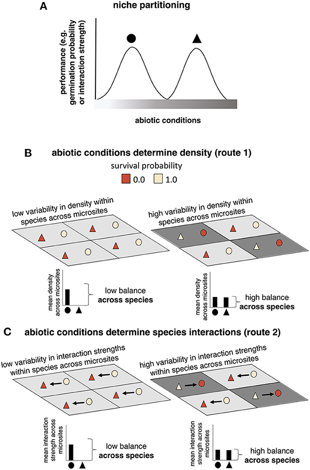
Figure 1. The two routes of abiotic influence under niche partitioning. In (A) we introduce a simple community of two species, circles and triangles, with unique responses to an abiotic factor. In (B), we show how those unique responses influence the initial density of species in a landscape with low compared to high abiotic heterogeneity. Both landscapes have four “patches” that correspond to microsites with abiotic conditions shown in grayscale. The landscape with low abiotic heterogeneity is on the left and does not include any patch in which the triangle species can germinate. The landscape with high abiotic heterogeneity is on the right and includes patches where either circles or triangles can germinate depending on abiotic conditions. In the low heterogeneity landscape, triangles die everywhere and circles survive everywhere, resulting in low variability in density for each species across the landscape. In the high heterogeneity landscape, circles and triangles both die in some patches but germinate in others, resulting in high variability in density for each species across the landscape. Below each landscapes we quantify the mean density across microsites experienced by each species. When species have different means we can say there is low balance across species, and high balance when their means are similar. In (C), abiotic conditions affect interaction strengths between germinated seedlings, shown as arrows, instead of density, but predicted effects are the same as discussed above for (B). Individuals colored dark red are present as seeds but either cannot germinate (B) or germinate but die later during competitive interactions (C).

Since heterogeneity-diversity relationships (HDRs) are recognized as an important diagnostic and guide for conservation and restoration practitioners, previous work has focused on understanding the factors that determine their presence and shape (Lundholm, 2009; Stein et al., 2014; Ben-Hur and Kadmon, 2020). Two oft-invoked reasons why HDRs may not be found, even when species are known to have different niches, are (1) dispersal—either too little, such that species don't have access to their niche (Lundholm, 2009); or too much, such that species in sink habitats persist via subsidies from source habitats (Shmida and Wilson, 1985; Leibold et al., 2004), and (2) the relative strength of intra- and interspecific competition, wherein local coexistence is possible even in landscapes with low abiotic heterogeneity if the species occurring within its preferred environmental conditions experiences strong intraspecific competition (Chesson, 2000). Configurational and compositional heterogeneity (i.e., variability in spatial autocorrelation and the range of environmental conditions, respectively) are also important factors shaping HDRs (Ben-Hur and Kadmon, 2020), but are beyond the scope of the current study as we are primarily interested in biotic effects arising from variability in density and interaction strengths.

Effects of the abiotic environment on both density and interaction strengths influence competitive outcomes between species, and can thus shape variability in realized competition across a landscape. We refer hereafter to low variability in realized competition across species as “high competitive balance,” and high variability in realized competition across species as “low competitive balance.” Our choice to use the word balance is meant to emphasize that this is a measure of variability at the community level, distinct from the within-population competitive variability, illustrated as within-species variability in density in Figure 1B, commonly referenced in the coexistence literature (e.g., where competition that covaries with environment can contribute to a storage effect Chesson, 2000). Competitive balance across species can arise from either within-species variability in density (Figure 1B), and/or within-species variability in interaction strengths (Figure 1C). When abiotic heterogeneity is low, we expect competitive balance across species to be low because throughout the landscape one or a few species benefit from being in or near their optimal abiotic conditions, while the rest are at a disadvantage. When abiotic heterogeneity is high, we expect competitive balance to be high because all species benefit from optimal abiotic conditions in some areas, and are disadvantaged by sub-optimal abiotic conditions in others. We thus predict that increased competitive balance with increased abiotic heterogeneity will be a key variable structuring diverse communities.

Recent studies exploring the effect of environmental heterogeneity on community patterns have used spatial Lotka-Volterra ordinary differential equations wherein various parameters change along an environmental gradient (e.g., carrying capacity or competition coefficients in Liautaud et al., 2019, or competition coefficients and intrinsic growth rates in O'Sullivan et al., 2021). An important limitation of these studies is that they ignore the inherently step-wise temporal process of community assembly, where species arrive and establish at a site before they grow and interact with other established individuals. In other words, they do not account for differences in a species' regeneration niche, which may be very different from the conditions required for subsequent success during interactions affecting survival and growth (Grubb, 1977; Bell et al., 1999; Marques et al., 2014; Larson and Funk, 2016). We overcome this limitation by modeling differences in germination probability for a community of plant species, which affects whether a species can be present at all, and at what densities, in a location before competitive interactions occur.

Using an individual-based spatially explicit simulation model, we compared heterogeneity-diversity relationships (HDRs) generated when abiotic conditions influenced initial densities early on during germination, to HDRs generated when the same abiotic conditions had no effect on initial densities, but determined per capita interaction strengths later during competitive interactions. These simulations allow us to understand (and compare) HDRs that arise when the impact of the abiotic environment is negligible during all but one life history event (e.g., early, during germination, or later during competition). This represents the case when either some events are not strongly affected by abiotic conditions, or they are strongly affected by an abiotic factor that has little variation within the landscape. We expect that in many real communities, multiple events will be impacted by the abiotic environment, so we also simulated both early- and late-stage abiotic effects in combination. We were then able to use our initial simulations (in which only germination or only competition was impacted by abiotic conditions) to decompose the effects of each of these on local species richness patterns in the combined simulations compared to a null control where abiotic conditions had no effect on species performance. Our simulation design allowed us to evaluate multiple scenarios that had different degrees of complexity. Simulations encompassed cases where plants respond to a single abiotic factor (or two spatially correlated factors) across life stages, cases where plants respond to an abiotic factor that changes in spatial configuration over time (or to two abiotic factors that vary at different spatial scales), as well as cases where plants respond to two spatially uncorrelated abiotic factors that vary at the same spatial scale. We repeated all simulations across three dispersal distances and three different ratios of intra- to interspecific competition to assess the importance of each route of abiotic influence on HDRs in the presence of these other confounding processes.

2. Methods

A spatially explicit, individual-based simulation model adapted from Palmer (1992) was used to manipulate species responses to abiotic conditions at specific life stages. Simulations followed the same structure outlined in Palmer (1992), which we review below along with additional modifications. We then describe the manipulations that allowed us to examine how abiotic effects on variable density and per capita interaction strengths affected community patterns under various parameter combinations. Finally, we describe how simulation output was collected and analyzed. Simulations were conducted in Matlab (MATLAB, 2018). Data generated in Matlab were analyzed in R Core Team (2017).

2.1. The model

2.1.1. Abiotic landscapes

Plant dynamics were simulated on a landscape characterized by a set of three 65 x 65 matrices representing three abiotic factors (one factor is given as an example in Figure 2A). Values in one of the three matrices represented an abiotic factor that determined plant fecundity (hereafter called abiotic factor R for reproduction). Values in the other two matrices represented abiotic factors that determined germination probability and competitive outcomes (abiotic factors G and C for germination and competition, respectively). Throughout, we will use the label A to refer to these abiotic factors in the general sense (where our descriptions apply to any of the 3 landscapes), reserving the labels R, G and C for when we wish to refer specifically to the abiotic landscapes driving reproduction, germination, or competition, respectively. Abiotic landscapes were randomly generated and all had intermediate spatial autocorrelation (fractal dimension D = 2.5, see Supplementary Section 1.1 for more details on the spatial configuration of landscapes and Table 1 for a summary of all parameters). These three abiotic factor matrices can be, but need not be, distinct from one another. In all of our simulations, we set abiotic factor G = C = R except where noted. Each matrix element represented a microsite (x, y) (for x, y= 1, 2,…, 65), and each microsite had abiotic conditions G(x, y), C(x, y), and R(x, y) for the abiotic factors determining germination, competitive, and reproductive abilities, respectively. Microsites had a maximum occupancy of c = 3 individual plants, representing a set carrying capacity due to the finite size of the microsite.

FIGURE 2

Figure 2. When (A) abiotic conditions vary over a landscape, species performance, P_{A_l}, may (B) depend on abiotic conditions, or (C) be independent of abiotic conditions. Points in (D, E) represent individual plants and colors represent species visualized after 200 rounds of simulated dynamics where abiotic effects of landscape A_l influenced (D) density and (E) interaction strengths. Solid arrows map how species responded to the abiotic environment during early compared to late life stages (germination and competition, respectively) when abiotic conditions influenced initial densities (route 1). Dashed arrows show the same but for route 2, when abiotic conditions determined interaction strengths. Point pattern analysis (F) across parameter space [including point patterns shown in (D, E)] show that interspecific segregation and intraspecific clumping (quantified by the ISAR and PROP_con, respectively, Supplementary Table 1) were greater when abiotic conditions affected density compared to when they affected interaction strengths (lines are median values, and shaded areas are 1.5 times the interquartile range). ISAR and PROP_con values when abiotic effects were indirect overlapped with values from the null model that excluded effects of the abiotic environment on species performance. Point pattern maps (D, E) are from simulations with intermediate dispersal and α_ij = 1.0.

TABLE 1

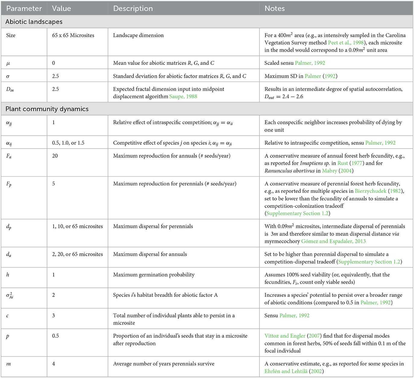
Table 1. Description of model parameters.

2.1.2. Simulating plant dynamics

We consider a model community consisting of two annual species and two perennial species. To begin each simulation, N_i = 1,056 (where N_i = landscape dimension squared, 65², divided by the number of species N_S = 4, rounded to the nearest integer) individuals of each species were randomly placed on a landscape. Once placed, individuals underwent an initial round of competition (as described below) until no microsite exceeded carrying capacity. In the first year, individuals surviving competition went on to a round of reproduction, dispersal, and mortality. At the beginning of every year after the first, seeds from the previous year germinated, followed again by competition, reproduction, dispersal, and mortality. As in Palmer (1992), the performance of any individual of species i at location (x, y) in response to abiotic factor A was calculated using a Gaussian function:

\begin{array}{l} P_{A i} (x, y) = exp (\frac{- {[A (x, y) - μ_{A i}]}^{2}}{2 σ_{A i}^{2}}) . & (1) \end{array}

μ_Ai is the niche optimum of species i (the value of abiotic factor A at which species i can achieve its peak performance) (Figure 2B). $σ_{A i}^{2}$ is the niche width of species i. We set the abiotic factor A(x, y) = G(x, y) to calculate the germination probability of an individual of species i, P_Gi. Likewise, performance during competition (P_Ci) and reproduction (P_Ri) were calculated using Equation (1) with A(x, y) = C(x, y) and R(x, y), respectively. Dispersal and non-competitive mortality of germinated individuals were modeled independently of the abiotic landscape (Table 1). In our model, annuals could never displace an adult perennial. Thus, when all else was equal, perennials tended to exclude the annuals from the landscape. In order to assess community patterns when both annual and perennial species co-occurred, we modeled trade-offs in colonization and dispersal ability such that annuals produced more seeds and could disperse farther than perennials. We chose values comparable to differences observed in commonly found annuals and perennials in forest herbaceous layer communities (Bierzychudek, 1982; Mabry, 2004) (Table 1). Below, we describe how we modeled competition and germination in detail, as they are the life stages of interest in our study. Further details about how we modeled reproduction, dispersal, and mortality can be found in the Supplementary Section 1.2.

Competition occurred only when microsite carrying capacity was exceeded. Within these microsites, randomly-placed individuals (in the first year) or germinating seedlings (in all subsequent years) of species j were removed according to probability r_j(x, y):

\begin{array}{l} r_{j} (x, y) = \frac{1}{Z} n_{j} (x, y) [α_{j j} n_{j} (x, y) + \sum_{i \neq j}^{N_{S}} α_{j i} P_{C i} (x, y) n_{i} (x, y)], & (2) \end{array}

Where n_i(x, y) is the pre-competition density of species i in microsite (x, y), N_S is the total number of species in the model, and Z is a normalization constant discussed below (Palmer, 1992). Values of α specify how strongly individuals affect conspecific (α_jj) and heterospecific (α_ji) neighbors in optimal abiotic conditions (i.e., the highest point of the Gaussian curve specified by Equation 1). The closer abiotic conditions C(x, y) are to the niche optimum of a competitor species i, the stronger the competitive effect of species i on species j and the higher the probability that species j does not survive the competitive interaction. Values of r_j(x, y) thus represent realized competitive effects on species j. As in Palmer (1992), per capita intraspecific competition was held constant at α_jj = α_ii = 1 and was assumed to be insensitive to the abiotic landscape. The latter assumption could be changed by multiplying the first term in the brackets in Equation (2) by a new performance function, P_Aj(x, y), and would lead perhaps to altered patterns, as we discuss below. Across simulations, we varied maximal per capita interspecific competition α_ji = α_ij to be either greater than, equal to, or less than intraspecific competition (Table 1). Since α_ji = α_ij and α_jj = α_ii = 1, we hereafter use the notation α_ij to refer to maximum baseline interspecific competition and α_ii to denote intraspecific competition. Except in the first year (when competition was imposed to establish initial conditions with ≤ c individuals per microsite), only germinating seedlings were affected by competition. Adults in a microsite exerted a competitive effect on germinating seedlings, but were not themselves affected by competition once established (Yu and Wilson, 2001). Probabilities r_j were calculated by first computing the numerator of Equation (2) for all competing species then normalizing by the constant Z necessary for these to sum to one. Removal probabilities were calculated once according to the total number of germinating individuals in the microsite, and then random numbers were drawn and individuals removed based on these initial probabilities until carrying capacity was reached.

The original model includes competition as described above, but no separate step determining germination probability (Palmer, 1992). To simulate abiotically-generated variability in initial densities, we added an additional step at the beginning of each growing season wherein viable seeds produced by species j in the previous year germinated according to probability:

\begin{array}{l} g_{j} (x, y) = h P_{G j} (x, y) . & (3) \end{array}

Setting h = 1 ensured that a seed in a microsite with optimal conditions G(x, y) = μ_Gj always germinated. In sub-optimal habitats (i.e., G(x, y)≠μ_Gj), germination depended on the outcome of random draws, as described above for determining competitive outcomes.

2.2. Experimental design

All simulations were carried out on 20 replicate landscapes (A_l, l = 1, 2, …, 20) to avoid results particular to a specific spatial configuration of the environment. In a simulation, species could either respond to abiotic conditions via niche partitioning (Figure 2B), or were indifferent to changes in abiotic conditions over the landscape (Figure 2C). We used the P_Ai(x, y) values from Equation (1) to simulate niche partitioning (species performance depended on abiotic conditions at location x, y). Niche optima were equally spaced along an abiotic factor niche axis, and standardized across abiotic factors by offsetting the optima of the first and last species by an amount determined by the range of abiotic conditions present in each landscape:

\begin{array}{l} μ_{A 1} = m i n A + \frac{m a x A - m i n A}{N_{S}} & (4) \end{array}

and

\begin{array}{l} μ_{A N_{S}} = m a x A - \frac{m a x A - m i n A}{N_{S}} . & (5) \end{array}

All other species were assigned optima at regular intervals between μ_A1 and μ_{A_N_S} (Figure 2B). Species niches therefore shifted depending on which replicate landscape they were in, but were identical across all simulations and treatments on that landscape. We define species j's preferred habitat as abiotic conditions A wherever P_Aj(x, y)>P_Ai(x, y) for all i≠j, including where P_Aj was low for species occupying end-range habitat. To model scenarios when performance did not depend on the abiotic environment, the expected ability for each species in a particular landscape was held constant at $\bar{P_{A j}}$ , a spatial average of P_Aj(x, y) across microsites and initial conditions from simulations with abiotic effects on both density and interaction strengths (Figure 2C). Spatial averages $\bar{P_{G j}}$ and $\bar{P_{C j}}$ were then normalized by dividing by the amount of preferred habitat available to each species in landscape matrix G and C. Although our model structure allows for the possibility of niche partitioning during reproduction, we opted to model fecundity as a spatial average across all simulations to simplify our analysis (details can be found in Supplementary Section 1.3). Note that although we exclude niche partitioning over space in the null model, species still differed in other aspects (e.g., perennials had lower fecundity and could not disperse as far as annuals).

Setting species performance to either P_Aj(x, y) or $\bar{P_{A j}}$ allowed us to turn niche partitioning on and off, respectively. To isolate abiotically-generated variability in density, we let abiotic conditions determine germination probability using Equation (3) as written, and turned abiotically-generated variability in interaction strengths off by replacing P_Ci(x, y) in Equation (2) with $\bar{P_{C i}}$ for all microsites (solid arrows leading from Figures 2B–D). Note that although we eliminate abiotically-generated variability in interaction strengths when $P_{C i} (x, y) = \bar{P_{C i}}$ in Equation (2), realized competition [r_j(x, y)] could still vary across the landscape because of differences in local densities. All simulations were similarly modified such that species responded to the abiotic environment either during germination to generate variability in density as described above, and/or during competition to generate variability in interaction strengths (dashed arrows leading from Figures 2B–E). To model a null control, germination probability and interaction strengths were both held constant at their spatial average for each species ( $P_{A j} (x, y) = \bar{P_{G j}}$ and $\bar{P_{C j}}$ , respectively). When we modeled the combined effects of variable density and variable interaction effects, we considered both the case where a single abiotic factor governed both germination and competition (G = C), and the case where germination and competition were governed by separate, uncorrelated factors (G independent of and ≠C). Scenarios were simulated nine times, for each parameter combination of dispersal distance (adjacent, intermediate, or universal) and strength of interspecific competition (α_ij < , =, or >α_ii) (Table 1). Simulations were run for 200 years, across the 20 replicate landscapes, with 5 random initial conditions (species placement in the first generation) per landscape. Every outcome in the model was stochastic and determined via random draws. The same sequences of random draws were replicated across simulations to ensure that observed differences in the outcomes of different simulations were due to differences in the scenario under consideration and not merely due to stochasticity. That is, even though simulated outcomes will of course be influenced by the specific stochastic perturbations imposed, we controlled for these influences by using the same sequences of perturbations across different simulated scenarios; remaining differences among scenarios must then be due to something else.

2.3. Analysis

Two community-level point pattern analyzes were used to assess differences in neighborhood spatial structure generated by route 1 and 2 compared to the null model: the Individual Species Area Relationship, ISAR(r), and the Proportion of conspecifics, PROP_con(r). The ISAR(r) is a distance-based measure of how segregated or intermingled members of different species are in neighborhoods of radius r around an average focal individual (Wiegand and Moloney, 2013). The PROP_con(r) is also distance-based, and measures how clumped or overdispersed conspecifics are around an average focal individual (Brown et al., 2016) (Supplementary Table 1). To eliminate edge effects we measured spatial statistics to a maximum radius of 10 microsites and never used individuals within 10 microsites of the landscape edge as focal individuals (Wiegand and Moloney, 2013). Spatial statistics were averaged across initial conditions and landscapes across all parameters, as well as separately for each combination of parameters. Confidence envelopes were drawn by calculating 1.5 times the interquartile range around the median at each radius. As long as confidence envelopes did not intersect, we concluded that differences in the resulting spatial structure were significant.

Next, we split each landscape l into 169 sampling units (non-overlapping neighborhoods of 5 x 5 microsites). Using these sampling units as our scale of observation, we measured three key variables. The first two, total number of species present (species richness, S) and variability in abiotic conditions (v(A)), were used to measure heterogeneity-diversity relationships (HDRs). Since both density and interaction strengths affect competitive outcomes, we also calculated competitive balance (C_bal) across species by first taking the average competition experienced by newly germinated seedlings of a species j, $\bar{r_{j}}$ , and then getting the variability in $\bar{r_{j}}$ across all species in the sampling unit, $v (\bar{r_{j}})$ . To make C_bal more intuitive, we subtracted all values from the maximum observed over all simulations so that values increased with increasing balance (Supplementary Table 1). Across a sampling unit, low competitive balance thus indicates that some species are more affected by competition than others, while high competitive balance indicates that all species are similarly affected by competition (Figure 1). All values calculated for a sampling unit were averaged over initial conditions (for a total N = 20*169 = 3,380 data points per simulation from across the 20 replicate landscapes). Sampling units with only one species of germinating seedlings were dropped from analyzes that included competitive balance. To quantify broader-scale effects, we also compared how total species richness changed across the landscape when the range of abiotic conditions was restricted (σ = 0.5 instead of 2.5 for landscapes with intermediate dispersal and α_ij = α_ii), simulating an overall reduction in niche space that is likely to accompany processes like habitat loss and landscape homogenization (Thompson et al., 2013; Groffman et al., 2014).

Generalized linear mixed-effect models were used to quantify relationships between species richness (S), abiotic heterogeneity (v(A)), and competitive balance (C_bal) for routes 1, 2, and the null model. All mixed-effect models included landscape l as a random effect. HDRs were quantified as the magnitude of the fixed effect regression coefficient from models with abiotic heterogeneity as the fixed effect predicting species richness. To understand the joint effects of abiotic heterogeneity and competitive balance on species richness, we used the same method to quantify the relationship between abiotic heterogeneity and competitive balance, as well as for the relationship between competitive balance and species richness. Data from the nine parameter combinations of dispersal distance and strength of interspecific competition were modeled separately. Under niche partitioning, we expect to find positive HDRs, a positive relationship between abiotic heterogeneity and competitive balance, and a positive relationship between competitive balance and species richness (Figure 1). Finally, we used linear models to determine how much variance in the strength of each relationship was explained by route of abiotic influence, dispersal distance, strength of interspecific competition, and any significant interactions between them. We report variance explained as a percentage calculated using the sum of squares. Further details about the statistical models can be found in the Supplementary Section 1.4.

To assess the relative contributions of abiotically-generated variability in density and per capita interaction strengths to species richness patterns, we applied a method that leverages simulation model output to partition contributions from different mechanisms to a response variable of interest [described in detail in Ellner et al. (2019) and illustrated in Supplementary Figure 1]. In the present study, we partitioned contributions from abiotic routes of influence 1 and 2 to net changes in species richness, i.e., how many species were gained or lost, averaged across initial conditions and sampling units within replicate landscapes. Briefly, independent contributions from routes 1, r1, and 2, r2, are first estimated as the mean number of gains or losses of species in a sampling unit compared to mean richness observed in the null model simulations (red and yellow bars in Supplementary Figure 1A). Differences between the observed effect of routes 1 and 2 acting simultaneously and their predicted additive effect, r1+r2 (gray bar in Supplementary Figure 1A) tell us the non-additive effects of the two mechanisms combined, r1r2 (orange bar in Supplementary Figure 1A). Allowing routes 1 and 2 to act simultaneously but according to spatially uncorrelated landscapes lets us further partition the non-additive interaction effect into a component attributed to independent variance of routes 1 and 2, r1#r2, and a component attributed to the co-variance of routes 1 and 2, (r1r2) (beige and white bars in Supplementary Figure 1A). For the results, we illustrate contributions as stacked bars excluding the baseline null model (as illustrated in Supplementary Figures 1B, C). This procedure was repeated for each combination of dispersal and strength of interspecific competition (Table 1). Because contributions from different mechanisms are predicted to change across spatial scales (Wiens, 1989; Levin, 1992), this analysis was repeated using micro (1 x 1 microsites) and large (13 x 13 microsites) sampling units for comparison against our baseline of small (5 x 5 microsite) sampling units.

3. Results

3.1. Local patterns and spatial structure of simulated communities

Variability in density and variability in interaction strengths, although generated by identical abiotic environments, resulted in different community patterns (e.g., Figure 2D compared to Figure 2E). Within small sampling units (5 x 5 microsites), species richness and competitive balance were 1.3 and 1.2 times lower, respectively, when abiotic conditions determined initial densities during germination (route 1) than when abiotic conditions determined interaction strengths during competition (route 2) (mean species richness = 2.53 and 3.37, and mean competitive balance = 0.41 and 0.48, respectively, dashed lines in Figures 3A, B). Competitive balance was never lower than 0.26 and rarely decreased below 0.40 in simulations of route 2, but spanned the full range of values down to 0.00 in simulations of route 1 (Figures 3A, B). Similar to route 2, sampling units in the null model had mean species richness = 3.50 with competitive balance ranging between 0.28 and 0.49 (mean value = 0.48, Figure 3C). These differences are reflected in the point pattern analysis, where abiotic effects on density resulted in local biotic neighborhoods with higher interspecific segregation and intraspecific clumping than null model simulations (Figure 2F). Abiotic effects on interaction strengths resulted in local biotic neighborhoods that were not significantly different from those generated in the null model simulations (Figure 2F). Qualitatively these findings held for all parameter combinations except for adjacent dispersal and strong interspecific competition, in which route 2 resulted in significantly more spatial structure than the null model, but still significantly more interspecific mingling and less intraspecific clumping than when abiotic conditions influenced pre-competition densities (Supplementary Figures 2, 3).

FIGURE 3

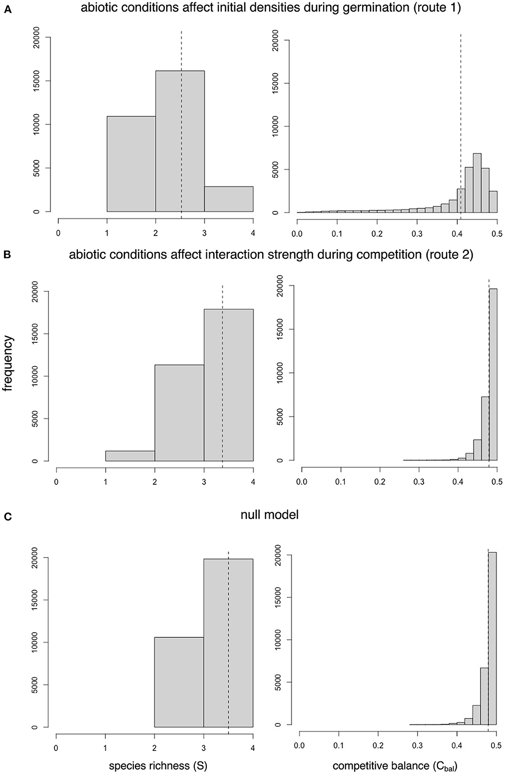
Figure 3. Histograms of species richness and competitive balance measured in small sampling units (5 x 5 microsites) across all parameter combinations from (A) simulations of abiotic effects on initial densities during germination (route 1), (B) simulations of abiotic effects on interaction strengths during competition (route 2), and (C) null model simulations when germination and competition were insensitive to changes in abiotic conditions. Dashed lines show mean values.

3.2. Landscape-scale species richness patterns

Although community patterns under route 2 look like those generated by the null model, a reduction in niche space (achieved by reducing the standard deviation of abiotic conditions across the landscape from σ = 2.5 to σ = 0.5) still reduced total species richness at the landscape scale when abiotic conditions determined interaction strengths, whereas total species richness in the null model was unaffected [SS = 4.51, DF = 1, F = 25.69, and P < 0.001 for the interaction between route of abiotic influence and standard deviation of abiotic conditions in the landscape (σ), Figure 4 and Supplementary Table 2].

FIGURE 4

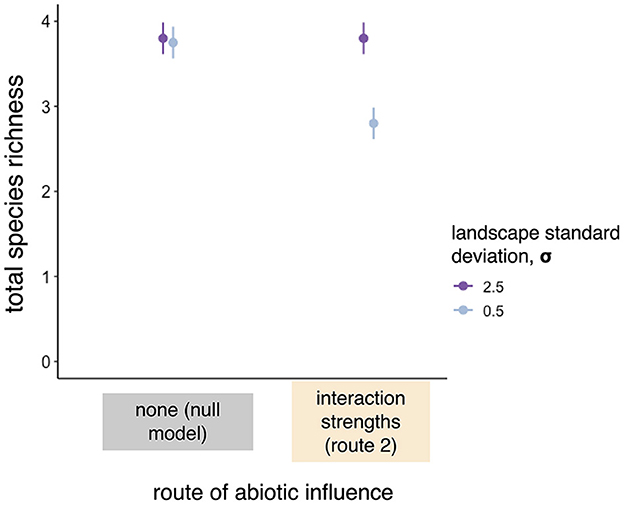
Figure 4. When we reduced the landscape-level standard deviation of abiotic conditions from 2.5 to 0.5, total species richness at the landscape-scale remained high in null model simulations, but decreased when abiotic conditions determined interaction strengths (route 2). Simulations had intermediate dispersal and α_ij = α_ii = 1. Points and whiskers are the estimated marginal means and confidence intervals from a linear model (Supplementary Table 2).

For all other analyzes when σ = 2.5, landscapes usually retained all 4 species regardless of the variable community patterns we found at local spatial scales (e.g., those reported across 5 x 5 microsite sampling units or within a 10 microsite radius for the spatial point pattern analyzes). Single species occasionally went extinct in the null model, and these losses were mitigated to various degrees when we introduced niche partitioning in subsequent simulations. Whenever species partitioned resources during germination, extinction never occurred (route 1 and simulations of route 1 in combination with route 2 in Supplementary Figure 4). Under route 2 when species only partitioned resources during competition, extinction was prevented 75% of the time when dispersal was adjacent and interspecific competition >0.5, 25% of the time when dispersal was intermediate and interspecific competition >1.0, and at least 11% of the time when dispersal was universal and interspecific competition was >0.5 (route “none” compared to route 2 in Supplementary Figure 4).

3.3. Relationships between abiotic heterogeneity, competitive balance, and species richness measured in small sampling units

When abiotic conditions determined initial densities during germination (route 1), we found positive heterogeneity-diversity relationships (HDRs) (Supplementary Table 3), positive relationships between abiotic heterogeneity and competitive balance (Supplementary Table 4), and positive relationships between competitive balance and species richness (Supplementary Table 5). When abiotic conditions determined interaction strengths during competition (route 2), we found flat HDRs and no relationship between abiotic heterogeneity and competitive balance (Supplementary Tables 3, 4), and strong positive relationships between competitive balance and species richness as long as dispersal was not universal (Supplementary Table 5). Figures 5A–C plot model predictions from simulations with intermediate dispersal and α_ij = α_ii as examples to illustrate these differences arising from route 1 and 2. In Figure 5A, the positive HDR arising from route 1 was 14 times stronger than the HDR arising from route 2, which was flat and not statistically significantly different from 0 (coefficient = 0.14 and 0.01, χ² = 172.15 and 0.17, DF = 1, P < 0.001 and = 0.68, respectively, Supplementary Table 3). Similarly, an increase in abiotic heterogeneity led to an increase in competitive balance under route 1 but not under route 2 (coefficient = 0.02 and 0.00, χ² = 114.39 and 2.68, DF = 1, P < 0.001 and = 0.1, respectively, Figure 5B and Supplementary Table 4). When dispersal was restricted to adjacent microsites and interspecific competition was stronger than intraspecific competition (α_ij = 1.5), route 2 led to a statistically significant positive HDR (coefficient = 0.04, χ² = 24.17, DF = 1, P < 0.001, Supplementary Figure 5A and Supplementary Table 3). However, the coefficient for route 1 under the same parameters was 5.9 times larger (coefficient = 0.21, χ² = 418.22, DF = 1, P < 0.001, Supplementary Table 3), and abiotic heterogeneity was not a statistically significant predictor of competitive balance (coefficient = 0.00,χ² = 1.18, DF = 1, P = 0.28, Supplementary Table 4). When slopes arising from route 2 were significantly different from 0 under intermediate and universal dispersal they were at least 8 times smaller than the slopes arising from route 1 (an example is plotted in Supplementary Figure 5B). Finally, Figure 5C shows that with intermediate dispersal and α_ij = 1.0, an increase in competitive balance led to a statistically significant increase in species richness under route 1 (coefficient = 3.09, χ² = 241.25, DF = 1, P < 0.001, Supplementary Table 5), and a marginally significant increase under route 2 (coefficient = 2.72, χ² = 3.40, DF = 1, P = 0.07, Supplementary Table 5). When dispersal was universal, the relationship between competitive balance and species richness weakened. Supplementary Figure 5C shows an example where the strength of the effect of competitive balance on species richness arising from route 1 was 5.8 times larger than the effect arising from route 2 when dispersal was universal (coefficient = 3.86 and 0.66, χ² = 253.36 and 0.75, DF = 1, P < 0.001 and = 0.22, respectively, Supplementary Table 5).

FIGURE 5

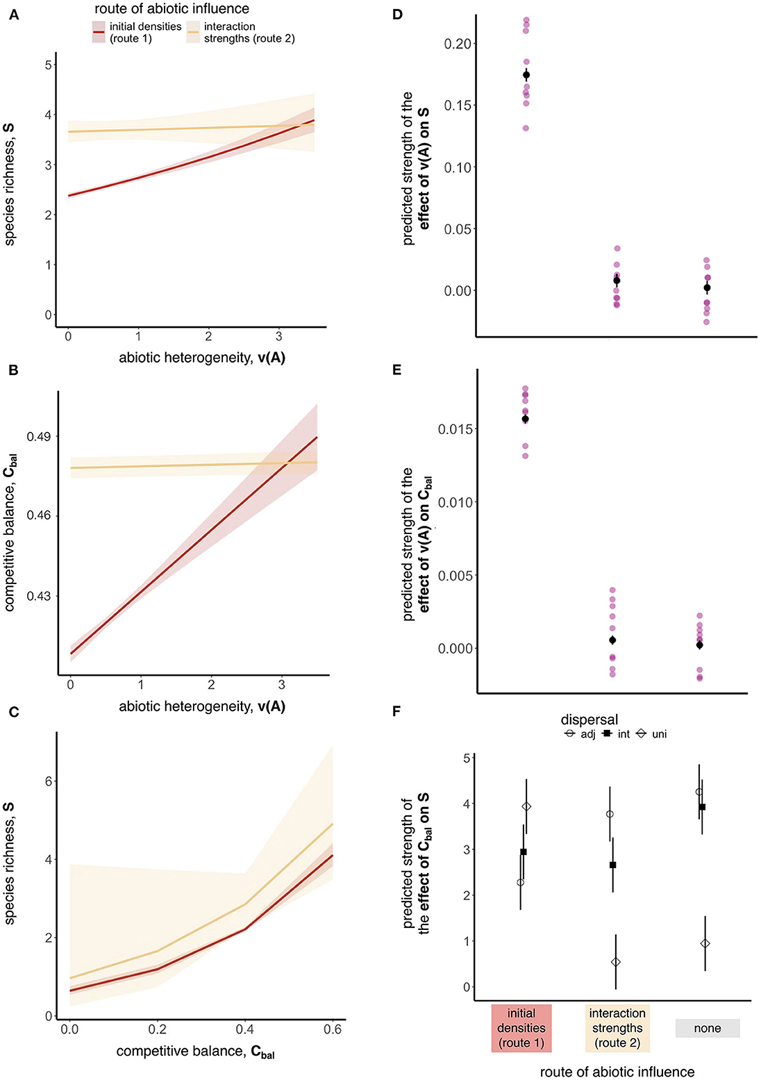
Figure 5. Relationships between abiotic heterogeneity and species richness (row 1), abiotic heterogeneity and competitive balance (row 2), and competitive balance and species richness (row 3) when abiotic conditions influenced initial density during germination (route 1) or interaction strengths during competition (route 2). As an example, (A–C) show generalized linear mixed-effect model (glmer) predictions for simulations with intermediate dispersal and α_ij = α_ii. Shading around predicted values are 95% confidence intervals. (D–F) Capture average trends across parameter combinations (i.e., lighter data points in (D, E) are fixed effect coefficients from a glmer model, while the darker points and whiskers are estimated marginal means and 95% confidence intervals from the linear model). (D, E) Show the main effect of route of abiotic influence on predicted relationship strengths. (F) Shows the interaction effect of route of abiotic influence and dispersal on the fixed effect coefficients from the effect of competitive balance on species richness and for clarity shows only estimated marginal means and 95% confidence intervals. We decided not to plot the interaction effect in (D) because, although statistically significant, it explained less than 2% of the variation in relationship strength (Table 1). Predictions in (E) come from a linear model excluding an interaction (see Supplementary Section 1.4). All data were measured in small sampling units (5 x 5 microsites).

Over all parameter combinations, route 1 consistently led to stronger HDRs (SS = 0.08, DF = 2, F = 634.39, P < 0.001, Figure 5D) and stronger relationships between abiotic heterogeneity and competitive balance (SS = 0.00, DF = 2, F = 3438.7, P < 0.001, Figure 5E) compared to route 2 (Table 2). The relationship between competitive balance and species richness was best explained by an interaction between route of abiotic influence and dispersal, where the relationship was strong regardless of abiotic route of influence when dispersal was restricted, but weakened when abiotic conditions affected interaction strengths and in the null model when dispersal was universal (SS = 26.5, DF = 4, F = 28.8, P < 0.001, (Figure 5F and Table 2). The statistically significant interaction between route of abiotic influence and dispersal distance explained 49.2% of the variation in the strength of the relationship between species richness and competitive balance (Table 2). The interaction between route of abiotic influence and dispersal was also statistically significant for the HDR (SS = 0.00, DF = 4, F = 12.2, and P < 0.001). Dispersal and its interaction with abiotic route of influence explained 2.8% and 1.6% of the variability in HDR strength, respectively, while the main effect of route of abiotic influence explained 41.4% (Table 2).

TABLE 2

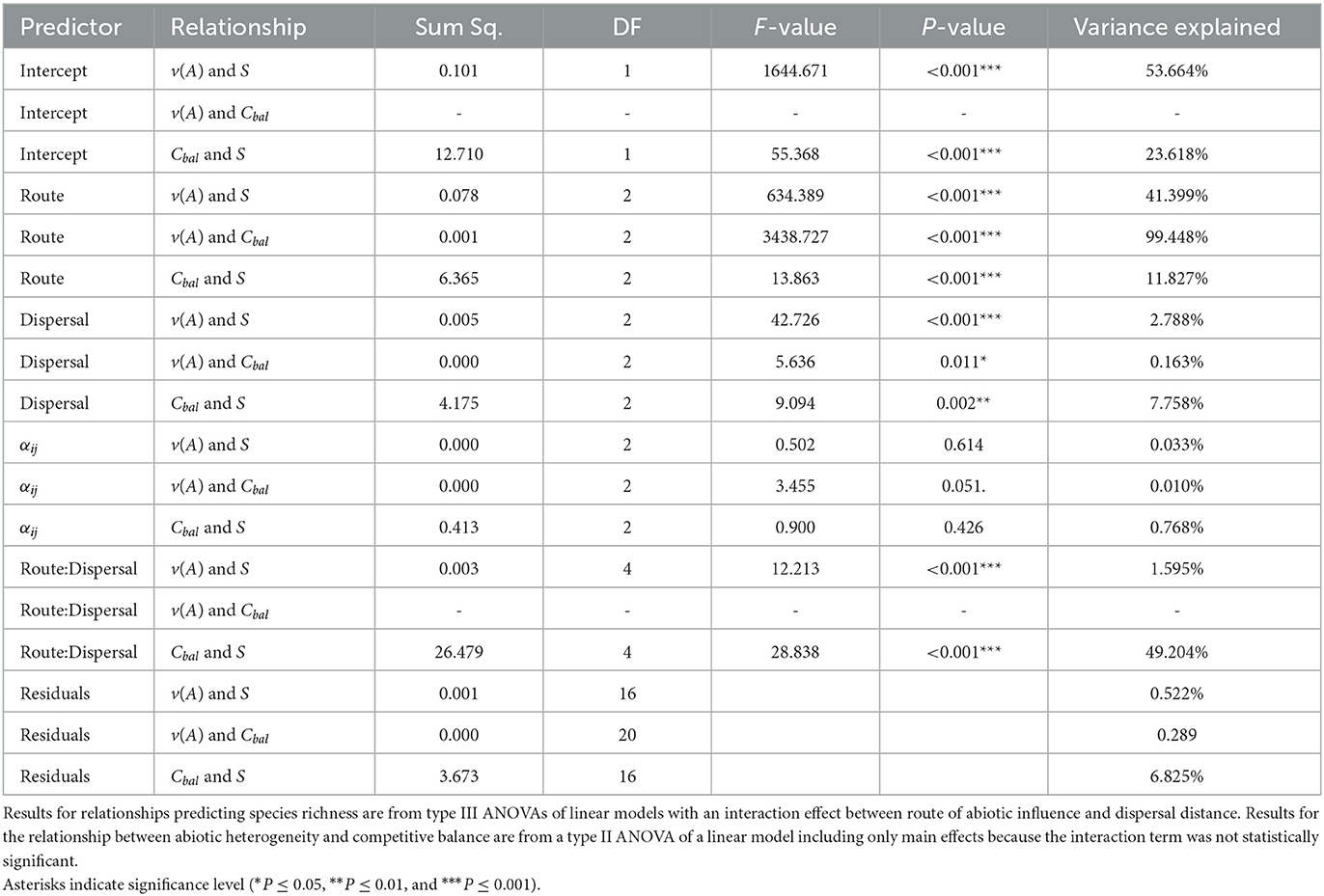
Table 2. Route of abiotic influence (on density, interaction strengths, or neither in the null model) was always a significant predictor of the strength of the measured relationships.

3.4. Decomposing combined effects of abiotically-generated variability in density and interaction strengths across sampling scales

Compared to the null model, independent contributions from abiotic effects on initial densities (route 1) and on interaction strengths (route 2) both led to net loss in average number of species in microsites and small sampling units (5 x 5 microsites) (Figure 6 and Supplementary Figure 6). For route 1, average species loss decreased from 1.34 under adjacent dispersal, to 1.16 and 0.57 under intermediate and universal dispersal, respectively. For route 2, average species loss also decreased with increased dispersal distance, from a maximum loss of 0.53 when dispersal was adjacent to a maximum loss of 0.07 when dispersal was universal. Additionally for route 2, net loss increased by a factor of 8.8 with increased strength of interspecific competition when dispersal was adjacent, by a factor of 13 when dispersal was intermediate, and a factor of 3.5 when dispersal was universal. In large sampling units (13 x 13 microsites), route 2 led to small gains in species richness compared to control simulations, with a maximum average gain of 0.07 when dispersal was universal and interspecific competition was strong (Supplementary Figure 6). Spatially correlated contributions from routes 1 and 2 led to more species loss than expected if effects were additive. These non-additive effects increased with increasing strength of interspecific competition from 0.10 to 0.23 when dispersal was adjacent, from 0.06 to 0.15 when dispersal was intermediate, and from 0.06 to 0.17 when dispersal was universal (white bars in Figure 6B). Spatially uncorrelated contributions were also non-additive but led to species gains instead of losses, which increased with increased strength of interspecific competition from 0.06 to 0.48 when dispersal was adjacent, from 0.03 to 0.11 when dispersal was intermediate, and from 0.03 to 0.04 when dispersal was universal (beige bars in Figure 6B). Observed changes in contributions were qualitatively similar across spatial scales of observation (except where noted for route 2 under universal dispersal), and contributions were largest in small sampling units (Supplementary Figure 6).

FIGURE 6

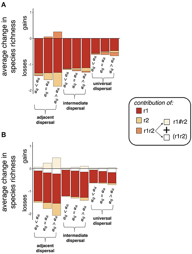
Figure 6. Abiotic effects on density (route 1) and interaction strengths (route 2) both led to species losses in small sampling units (5 x 5 microsites). Contributions from route 1, r1, were generally larger than contributions from route 2, r2. In (A), we can see that contributions from the interaction between routes 1 and 2, r1r2, were usually small. In (B), we can see this is because the uncorrelated (“r1#r2”) and correlated [“(r1r2)”] components of r1r2 had opposite effects on species richness. Specifically, uncorrelated contributions resulted in species gains, while correlated contributions resulted in species losses.

4. Discussion

We initially hypothesized that both routes of abiotic influence would generate positive heterogeneity-diversity relationships (HDRs), but our results do not support this prediction. We found that positive HDRs only occurred when abiotic conditions influenced initial density (route 1), simulated here as an abiotic effect on germination probability. When the same abiotic conditions determined interaction strengths during competition (route 2), we found no relationship between abiotic heterogeneity and species richness (flat HDRs) because sampling units with low abiotic heterogeneity could still support high species richness when abiotic conditions affected interaction strengths, but not when they affected densities (e.g., sampling units with v(A) < 2 in Figure 5A). We also initially hypothesized that positive HDRs arise through either (or both) of two related mechanisms. First, increased abiotic heterogeneity increases niche availability, creating the possibility for more species to be present in a given area. Second, increased abiotic heterogeneity increases competitive balance by increasing either variability in density within species (Figure 1B) and/or variability in interaction strengths within species (Figure 1C). However, we found that a positive relationship between abiotic heterogeneity and competitive balance only occurred when abiotic conditions influenced initial densities (route 1), not when abiotic conditions determined interaction strengths (route 2) (Figure 5E and Supplementary Table 4). As with HDRs, this was because sampling units with low abiotic heterogeneity still had high competitive balance when abiotic conditions affected interaction strengths, but not when they affected densities (e.g., sampling units with v(A) < 2 in Figure 5B).

Under route 2, germination is guaranteed across abiotic conditions but survival hinges on competitive dynamics, suggesting two possible explanations for the high species richness in sampling units with low abiotic heterogeneity. First, we made local coexistence easier to achieve whenever α_ij ≤ α_ii. Even when α_ij>α_ii, sub-optimal abiotic conditions could still reduce interspecific interaction strengths. Thus it may be that only strong destabilizing mechanisms will result in competitive exclusion in areas with low abiotic heterogeneity, which explains why we observed an increase in small local losses with increased interspecific competition (Figure 6). Since intraspecific competition tends to be more strongly limiting than interspecific competition when competitors partition resources (Adler et al., 2018), we think that considering these scenarios reported here where interspecific competition tends to be weaker than intraspecific competition may be especially relevant to real communities. A second explanation for high species richness in sampling units with low abiotic heterogeneity is that route 2 allows species to utilize empty space anywhere on the landscape. For example, since there are no abiotic restrictions on germination ability under route 2, species can thrive anywhere competitors are absent, including in areas where they would have been unable to germinate under route 1 (Kraft et al., 2015).

Although there was no signal for niche partitioning during route 2, a reduction in niche space still resulted in lower regional diversity than in the null model (Figure 4). This means that even if a species is unable to exclude an interspecific competitor in areas where it is competitively superior (either because its competitive effect is not strong enough or because it cannot occupy every open microsite), it still relies on these areas to persist. Stated another way, abiotically-generated variability in interaction strengths contributed to regional diversity even when it did not translate to differences in competitive balance. This is possible because in our model, competitive balance depended on both density and interaction strengths. Under route 2, density was independent from direct effects of abiotic conditions, but could still vary due to dispersal, stochasticity, or indirect effects of interaction strengths (for example when competitive exclusion did occur). As such, interaction strengths varied with abiotic conditions and contributed to regional maintenance of biodiversity, while competitive balance was determined by density and thus did not reflect differences in abiotic heterogeneity.

We initially hypothesized that strong or weak dispersal could obscure heterogeneity-diversity relationships (HDRs) due to either mass effects (Leibold et al., 2004) or an inability to reach preferred habitat (Lundholm, 2009), respectively. We found statistically significant effects of dispersal in the model for HDRs, but they never explained more than 3% of the variation in relationship strength. On the other hand, route of abiotic influence explained over 41% (Table 2). Although effects of dispersal on HDRs were weak compared to the effect of abiotic influence, we found that universal dispersal did reduce average species loss compared to the null model for routes 1 and 2 across all measured spatial scales (Figure 6 and Supplementary Figure 6), supporting the prediction that dispersal can mitigate local losses (Liao et al., 2013, 2016; Ramos et al., 2018). However, we found that when there was an interaction between routes 1 and 2, universal dispersal had the opposite effect and instead increased average species loss compared to the null model across sampling scales, (orange bars in Figure 6A and Supplementary Figure 6A), which occurred because uncorrelated effects of route 1 and 2 that led to more species when dispersal was adjacent led to no net change or fewer species when dispersal was universal (beige bars in Figure 6B and Supplementary Figure 6B). We hypothesize that this occurs because adjacent dispersal concentrates seed input, increasing the chances for a species with low germination probability to persist in that area.

As expected under coexistence theory, adding niche partitioning mitigated landscape-level extinctions that occurred occasionally in the null model (Supplementary Figure 4). One hundred percent of landscapes that lost a species in the null model retained that species when abiotic conditions affected initial densities (route 1). Mitigation was weaker when abiotic conditions affected interaction strengths, and depended on dispersal distance as well as strength of interspecific competition (Supplementary Figure 4). These results are in agreement with findings from Chu and Adler (2015) that show that niche partitioning during germination contributed more strongly to species coexistence than niche partitioning during competition.

4.1. Implications

When studies find no evidence for a heterogeneity-diversity releationship (HDR), three main alternative hypotheses tend to be invoked: (1) dispersal maintains populations of species outside their niche (Shmida and Wilson, 1985; Mouquet and Loreau, 2003), (2) the abiotic factor of importance varies at a different spatial scale than the scale at which the study was conducted (Lundholm, 2009), or (3) species are not partitioning the measured abiotic factor. Our results suggest a fourth alternative, which is that species do have differential responses to the measured abiotic factor, but its effects mediate interaction strengths rather than initial density. This fourth possibility has two unique consequences for restoration and conservation practitioners. First: biased detection of HDRs could overemphasize the importance of preserving or creating heterogeneity in abiotic conditions that affect density (i.e when the abiotic environment alters germination probability), when variable competitive environments may also contribute to both local and regional species richness. Second: communities where abiotic factors determine interaction strengths (route 2), although lacking a signal for niche partitioning, may still be susceptible to biodiversity loss with a reduction in niche space (Figure 4). Route 2 simulates a scenario where the abiotic factor determining germination probability varies at a larger spatial scale than the factor determining interaction strengths (i.e., germination probability remains constant because our sampling scale does not capture variability in the abiotic factor affecting germination). Thus, our results suggest that conserving/restoring abiotic heterogeneity at small spatial scales is equally important as conserving/restoring abiotic heterogeneity at large spatial scales. Our recommendation is to focus on nested levels of abiotic heterogeneity in both conservation and restoration. However, some care needs to be taken in balancing this recommendation with findings that high abiotic heterogeneity from the inclusion of extreme abiotic conditions can decrease species richness (for example due to inclusion of inhospitable conditions, as discussed in Yang et al., 2015).

4.2. Limitations and future directions

Following Palmer (1992), per capita strength of intraspecific competition was held constant in our model, but abiotic conditions could affect both intra- and interspecific competition. This could be accomplished by multiplying the first term in brackets of Equation (2) (the probability that species j dies) by an additional performance function, P_Aj(x, y), reflecting the impact of abiotic conditions of a landscape A on intraspecific competition (which could be the same as, or distinct from, the interspecific performance function P_Cj(x, y), depending on ecological context). If abiotic conditions in a given microsite favored species 1 and hindered species 2, then species 1 would not only have a strong effect on species 2, but also be strongly self-limited. Similarly, species 2 would not only have a weak effect on species 1, but also benefit from reduced self-limitation. How these trade-offs in competitive effect on heterospecifics and strength of self-limitation might affect competitive balance in sampling units with different levels of abiotic heterogeneity is an interesting question for future research.

Although the questions posed are relevant across taxa, our model and choice of parameter values speak most directly to a small understory community of annual and perennial plants (Table 1). An important goal for future research will be to determine how our findings change for larger communities containing species with different parameter combinations to simulate variability in trait composition. Due to interest in disentangling effects of density vs. interaction strengths (Chu and Adler, 2015; Hallett et al., 2019), we focused on effects of the abiotic environment on species density during germination compared to effects during competition on interaction strengths. However, abiotic conditions can affect species across a suite of life stages and interaction types. Abiotic effects on dispersal, for example, can vary considerably depending on the selective pressures facing species (Sullivan, 2014; LaRue et al., 2018). Indirect effects of abiotic conditions on dispersal is likely also common when they act via a mutualist, for example if the presence, abundance, or effectiveness of a dispersal mutualist depends on abiotic conditions (Lehouck et al., 2009). Regardless of the specificity of the model, our results highlight that niche partitioning does not always result in a strong correlation between abiotic heterogeneity and competitive balance, the process driving the landscape-level signature for niche partitioning [e.g., strong positive heterogeneity-diversity relationships (HDRs)]. We think this result is general because it is an extension of principles from coexistence theory (e.g., covariance between the environment and competition is a prerequisite for the storage effect, which concentrates species in their preferred habitats) (Figure 1). We therefore hypothesize that processes that strengthen the correlation between competitive balance and abiotic heterogeneity will strengthen the signal for niche partitioning, while processes that weaken that correlation will weaken the signal for niche partitioning. A clear future direction is to test this hypothesis across different life histories of diverse communities and taxa, and/or develop more general models to explore these relationships, since the present research demonstrates why it is difficult to predict a priori how abiotic effects will affect the correlation between abiotic heterogeneity and competitive balance.

5. Conclusions

Community-level signals for niche partitioning, e.g., positive heterogeneity-diversity relationships (HDRs), were evident when abiotic conditions affected germination probability and thus initial densities, but not when they affected interaction strengths during competition. When abiotic conditions affected germination probabilities, areas with low abiotic heterogeneity had low competitive balance and therefore low species richness. When abiotic conditions affected interaction strengths during competition, however, areas with low abiotic heterogeneity had high competitive balance and thus retained more species than expected, obscuring the expected positive HDR. Although the signal for niche partitioning was absent when abiotic conditions affected interaction strengths, a decrease in niche space still resulted in regional species loss. Therefore, we may not be able to identify which abiotic gradients support species richness in a landscape based on emergent patterns. Rather, it may be more informative to determine which abiotic factors drive differences in interaction strengths between species, for example based on functional traits and/or phylogeny. We conclude that understanding how abiotic heterogeneity affects biotic neighborhoods, and specifically competitive balance, will be a critical framework for linking species interactions to community-level patterns in future research.

Data availability statement

The datasets presented in this study can be found in online repositories. The names of the repository/repositories and accession number(s) can be found below: https://github.com/io-inspace/Abiotic-D-I-Effects.

Author contributions

SC developed the conceptual framework and questions, wrote the code, performed all analyzes, and wrote the initial draft of the manuscript. Both authors contributed to model building, contributed to editing it, contributed to the article, and approved the submitted version.

Funding

SC and KA were partially supported by the McDonnell Foundation Complex Systems Scholar grant #220020364. KA received additional support from NSF grant DMS-1840221.

Acknowledgments

We thank members of the Abbott Lab, Drs. Robin Snyder, Sara Kuebbing, and the Kraft Lab for their helpful comments on early manuscript drafts.

Conflict of interest

The authors declare that the research was conducted in the absence of any commercial or financial relationships that could be construed as a potential conflict of interest.

Publisher's note

All claims expressed in this article are solely those of the authors and do not necessarily represent those of their affiliated organizations, or those of the publisher, the editors and the reviewers. Any product that may be evaluated in this article, or claim that may be made by its manufacturer, is not guaranteed or endorsed by the publisher.

Supplementary material

The Supplementary Material for this article can be found online at: https://www.frontiersin.org/articles/10.3389/fevo.2023.1071375/full#supplementary-material

References

Adler, P. B., Smull, D., Beard, K. H., Choi, R. T., Furniss, T., Kulmatiski, A., et al. (2018). Competition and coexistence in plant communities: intraspecific competition is stronger than interspecific competition. Ecol. Lett. 21, 1319–1329. doi: 10.1111/ele.13098

PubMed Abstract | CrossRef Full Text | Google Scholar

Altamiranda-Saavedra, M., Osorio-Olvera, L., Yáñez-Arenas, C., Marín-Ortiz, J. C., and Parra-Henao, G. (2020). Geographic abundance patterns explained by niche centrality hypothesis in two Chagas disease vectors in Latin America. PLoS ONE 15, e0241710. doi: 10.1371/journal.pone.0241710

PubMed Abstract | CrossRef Full Text | Google Scholar

Bell, D. T., King, L. A., and Plummer, J. A. (1999). Ecophysiological effects of light quality and nitrate on seed germination in species from Western Australia. Aust. J. Ecol. 24, 2–10. doi: 10.1046/j.1442-9993.1999.00940.x