
95% of researchers rate our articles as excellent or good
Learn more about the work of our research integrity team to safeguard the quality of each article we publish.
Find out more
ORIGINAL RESEARCH article
Front. Ecol. Evol. , 14 March 2022
Sec. Behavioral and Evolutionary Ecology
Volume 10 - 2022 | https://doi.org/10.3389/fevo.2022.768478
This article is part of the Research Topic Cognitive Movement Ecology View all 16 articles
 Eliezer Gurarie1,2*
 Chloe Bracis3,4,5
 Angelina Brilliantova6,7
 Ilpo Kojola8Johanna Suutarinen8
 Otso Ovaskainen9,10,11
 Sriya Potluri2
 William F. Fagan2
The ability of wild animals to navigate and survive in complex and dynamic environments depends on their ability to store relevant information and place it in a spatial context. Despite the centrality of spatial memory, and given our increasing ability to observe animal movements in the wild, it is perhaps surprising how difficult it is to demonstrate spatial memory empirically. We present a cognitive analysis of movements of several wolves (Canis lupus) in Finland during a summer period of intensive hunting and den-centered pup-rearing. We tracked several wolves in the field by visiting nearly all GPS locations outside the den, allowing us to identify the species, location and timing of nearly all prey killed. We then developed a model that assigns a spatially explicit value based on memory of predation success and territorial marking. The framework allows for estimation of multiple cognitive parameters, including temporal and spatial scales of memory. For most wolves, fitted memory-based models outperformed null models by 20 to 50% at predicting locations where wolves chose to forage. However, there was a high amount of individual variability among wolves in strength and even direction of responses to experiences. Some wolves tended to return to locations with recent predation success—following a strategy of foraging site fidelity—while others appeared to prefer a site switching strategy. These differences are possibly explained by variability in pack sizes, numbers of pups, and features of the territories. Our analysis points toward concrete strategies for incorporating spatial memory in the study of animal movements while providing nuanced insights into the behavioral strategies of individual predators.
Spatial memory is fundamental to successful navigation of complex, dynamic environments (Fagan et al., 2013). Theoretical and simulation studies have shown that memory can be essential in structuring movements and space use (Mueller and Fagan, 2008; Barraquand et al., 2009; Van Moorter et al., 2009; Avgar et al., 2013; Watkins and Rose, 2013; Schlägel and Lewis, 2014; Bracis et al., 2015; Riotte-Lambert et al., 2017), and can help optimize resource acquisition in dynamic environments (Bracis et al., 2015, 2018). In parallel, movement data is rapidly accumulating. A central task of movement analysis is to infer behavioral mechanisms that underlie decision making processes (Nathan et al., 2008). Much effort has been devoted to inferring unobservable behavioral states from movement data (Morales et al., 2004; Forester et al., 2007; McClintock et al., 2012; Gurarie et al., 2016), while step and resource selection functions quantify animal movement responses to heterogeneous environments (Boyce and McDonald, 1999; Hebblewhite et al., 2005; Thurfjell et al., 2014). However, the underlying models almost always assume a straightforward, tactical response to immediate environmental cues, e.g., a fully informed preference for a particular habitat, or a probabilistic rule for switching behaviors under certain environmental conditions without accounting for memory driven responses. In fact, it has been demonstrated that not accounting for simple memory-based behavior can lead to misleading inferences in a step-selection framework (Van Moorter et al., 2013).
Despite the centrality of spatial memory and the abundance of movement data collected on animals in the wild, demonstrating that animals are using spatial memory is a surprisingly steep challenge. Many relevant studies have focused on terrestrial herbivores, which have the advantage of being relatively easy to study. Thus, bison (Bison bison) keep track of meadow patch locations and quality (Merkle et al., 2014, 2016), thereby constraining their space use in a way reminiscent of simulation-based predictions (Van Moorter et al., 2009). Migratory zebras (Equus zebra) demonstrate a memory-based anticipation of seasonal resource flushes (Bracis and Mueller, 2017), as do blue whales (Balaenoptera musculus) (Abrahms et al., 2019). Boreal woodland caribou (Rangifer tarandus caribou) movements can be modeled with respect to a stored estimates of forage quality and predation risk according to a nuanced cognitive model (Avgar et al., 2015). Recently used locations were among the most significant predictors of wild boar (Sus scrofa) movements and habitat use (Oliveira-Santos et al., 2016).
The herbivorous examples above feed primarily on stationary resources. In contrast, large carnivores feed on mobile and cryptic prey, which are themselves capable of spatial mapping and event-based memory when making movement decisions. This adds a non-trivial level of complexity to applying a foraging strategy. It is unclear, for example, whether predators should prefer or avoid locations where they were most recently successful. Re-use of those locations, referred to as “foraging site fidelity” is a suitable strategy if locations of recent success correlate with locations of future success. This hypothesis explains the large scale selection of foraging sites for several avian central-place predators (Davoren et al., 2003; Carroll et al., 2018). On the other hand, foraging site switching can occur if prey avoid an area where they have witnessed or are aware of the death of a conspecific. In this case, predators are best off changing the location where they predate, as had been demonstrated for lions (Panthera leo) in savannas (Valeix et al., 2011). Whether an immediate decision by a predator follows one strategy or another likely depends on the spatial scale of prey patches and foraging ranges, and on the temporal scale of prey patch persistence and depletion-recovery dynamics relative to the temporal scale of a predator foraging bout.
Wolves (Canis lupus) are highly adaptable, generalist, social predators of large prey. Their reproductive, hunting, territorial, seasonal, and dispersive behavior has been observed and described in great detail (Mech and Boitani, 2003), mainly in descriptive terms based on extensive field observations. Wolves are routinely described as having high cognitive abilities and complex information retention and communication skills. For example, Peters and Mech (1975) write that “Wolves appear to have well-organized memories for routes, points, junctions, and their juxtaposition,” and propose that the spatial distribution of wolf markings were a physical manifestation of their “cognitive maps.”
Despite this, compelling quantitative or model-based inference on the cognitive processes of wolf behavior in the wild has been elusive, in part because of the layered behavioral complexity of predator-prey interactions. In a recent study (Schlägel et al., 2017) winter wolf movements were modeled as a function of local prey density and boundary visitations, relating these to the time of return for each location as a indication of use of spatial memory. The results provide compelling evidence that wolves do track space and time. However, the modeling framework was constrained to a temporal scale fixed by the arbitrary sampling frequency of the GPS locations and a spatial scale of landscape rasterization fixed by computational limitations. The structure of the model thereby precluded an exploration of the temporal and spatial scales at which memory was operating.
Here, we develop, parameterize, fit, and explore a predictive, memory-driven model of spatial decision-making by wolves, focusing on the summer, den-centered, pup-rearing period. In this period, reproductive adult wolves must balance several important prerogatives: (1) they must hunt successfully, not just to feed themselves but to provide energetic surplus to pups, (2) they must regularly revisit the den to feed pups via regurgitation, and (3) they must periodically visit the edges of their territories to mark and patrol. The data we analyze were obtained from an intensive summer predation study contrasting established and dispersed packs of wolves in Finland, where wolves have reestablished themselves at relatively low densities via a process of natural dispersal from Russia (Kojola et al., 2006; Barry et al., 2020). During these predation studies, we obtained a detailed, behaviorally annotated time-series by visiting nearly all non-den GPS locations over a two-month period. Importantly, we identified carcasses, allowing us to infer the location, composition and timing of most kills (Gurarie et al., 2011), as well as boundary visits.
Our first goal was to demonstrate that wolves do use spatial memory by developing a cognitive model that outperforms a non-cognitive null model for predicting wolf foraging decisions. An important goal in developing the model was to have a heuristic that would allow us to estimate or approximate the temporal and spatial scales at which wolves weigh and act upon their recent predation success and boundary visitation. Once fitted, we anticipated that this model would provide insights into the fundamental decision-making strategies used by wolves to forage and maintain their territories.
Based on our knowledge of wolf behavior, we had several predictions: (1) that the valuing of predation might depend on the size of prey (e.g., an adult moose Alces alces being many magnitudes larger than a beaver Castor castor) and on the effort, in terms of time spent hunting, required to make a kill; and (2) that wolves would be inclined to return to territorial boundaries that had not been visited with some time lag to ensure they were marked, at a time lag approximately equal to the duration of a scent marking persistence. We also anticipated (3) that wolves would be more inclined to head toward (or value more highly) areas where they have had more recent predation success. We considered this more likely than site switching as the limited viewshed in forested environments may make it more difficult for prey to be aware of conspecific kills.
The study focused on eight summer-tracking studies of seven wolves in five unique territories in eastern Finland near the border with Russia (Figure 1). These territories are in the sparsely populated “core range” where wolves first recolonized Finland from Russia in the 1970's (Kojola et al., 2006), with primarily coniferous boreal forest dominated by Scotch pine (Pinus sylvestris), Norway spruce (Picea abies) and birch (Betula pendula and B. pubescens). As a result of extensive logging, clear cuts and young successional mixed forests are common. The landscape is further dotted with lakes and peat bogs, about half of which have been drained. Moose (Alces alces) and reindeer (Rangifer tarandus L.) are the two resident ungulate species in the study area (Kojola et al., 2004). Reindeer include the wild forest subspecies (R. t. fennicus) and the free-ranging semi-domesticated reindeer (R. t. tarandus). The distribution of wild forest reindeer is limited to the north by the area of semi-domesticated reindeer management, separated physically by a fence extending across Finland at roughly 65° N. North of this border, wolves have no legal protection and are commonly killed by local hunters (Kojola et al., 2006).
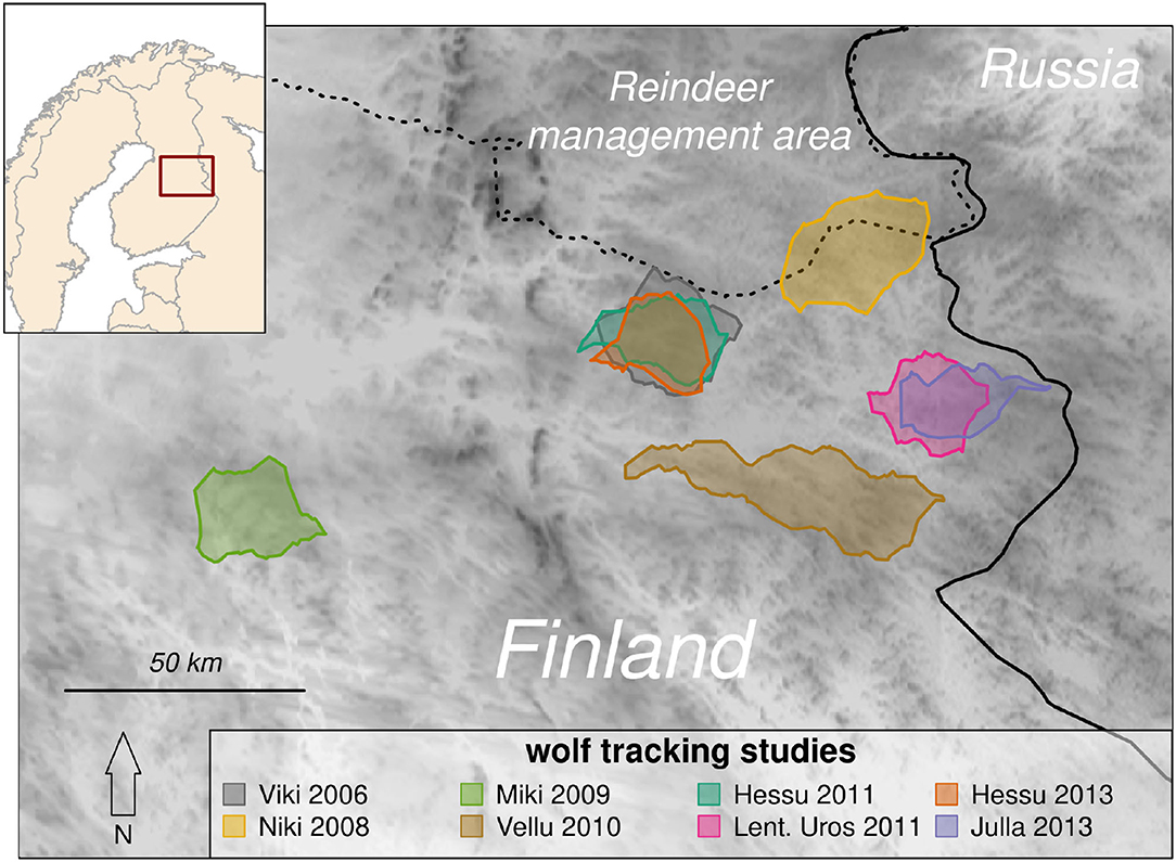
Figure 1. Map indicating the boundary polygons of eight wolf tracking studies in Finland (inset map). Several of the studies occurred in overlapping territories: Lentuan Uros's (magenta) territory in 2011 was inherited by Julla in 2013 (blue), and Viki's territory in 2006 was inherited by Hessu, who was tracked in 2011 and 2013 (gray, green, and orange). Darker colors on the map reflect higher elevations (maximum 340 m). These territories are in the core of the Finnish wolf range, near the border with Russia, whence the population naturally dispersed, but south of the reindeer management area (dashed line) which is separated from southern Finland by a fence north of which wolves are unprotected.
Wolves were captured and collared in late winter or early spring (between February and April) (Kojola et al., 2006). Individuals were captured using snowmobiles when the snow was soft and at least 80 cm. Snowmobiles were driven alongside wolves, which were looped using a neck-hold noose attached to a pole. The wolves were placed in a wooden box that had been strengthened with a metal grating around the outside and had doors at both ends. Wolves were kept in the box for at least 30 min before being injected with a mixture of medetodimine and ketamine with a dose ratio of 1:20 (Jalanka and Roeken, 1990). The wolves were equipped with collars that contained global positioning system receivers (GPS Plus 2, Vectronic Aerospace GmbH, Berlin, Germany) and Very High Frequency (VHF) radio beacon transmitters (Televilt, Lindesberg, Sweden). The collars weighed approximately 760 g and had expanding, adjustable collars. Capture, handling, and anesthetizing of the wolves met the guidelines issued by the Animal Care and Use Committee at the University of Oulu and permits provided by the provincial government of Oulu (OLH-01951/Ym-23).
We analyzed data from seven intensively field tracked wolves. Each wolf was followed intensively for 60 days from the beginning of June to the end of July for one summer each from 2006 to 2013, with the exception of one wolf (Hessu) that was followed for two summers (2011 and 2013). All of the collared wolves represented breeding individuals, and we did not have more than one wolf collared in any particular pack.
GPS locations were obtained for all the wolves at half hour intervals via the GSM (Global System for Mobile) network, which covered the entirety of all wolves' territories. In seven of the eight studies, every location was visited in the field after a minimum five day time lag, excluding locations near or around the den. The lag was maintained to minimize disturbance, and the locations visited on a given day were as far as possible from the location of the focal wolf on that day. The overall median lag was 8 days (inter-quartile range 5 to 11 days). A minimum radius of 25 m around each location was surveyed with the help of trained tracking dogs, who were able to efficiently identify signs of wolf presence, such as carcasses, caches, bedding sites, and scats. For the remaining study, only those locations that were clustered, corresponding to likely kill, bedding and cache sites, were visited. Cervid prey carcasses and age status (adult or calf) were identified by the bones and antlers. Several were not identifiable in the field, and were recorded as “unknown ungulate.” Other prey items, including hare (Lepus europaeus), beaver (Castor castor), capercaillie (Tetrao urogallus), black grouse (Tetrao tetrix) and one each of raccoon dog (Nyctereutes procyonoides), and Northern goshawk (Accipiter gentilis) were identified by pelage and plumage and classified as “minor” prey, with no further subdivision into age categories. For additional details on the field methodology, see (Gurarie et al., 2011), which provides a close analysis of the summer habitat preferences of two of the wolves. The simplified outcome of the intensive field tracking was a movement track annotated with behaviors, and location and identity of most prey consumed over the period of the studies. Separately, howling surveys (Fuller and Sampson, 1988) and winter tracking after each of the summer periods were used to estimate the number of adults, juveniles, and pups in each pack.
Our overarching goal was to specify and estimate a model that predicts the movement behavior of a wolf during the summer den-centered pup-rearing period. In summer, wolves expend considerable effort and energy on obtaining enough nutrition to feed and rear pups, leaving and returning to the den on a near daily basis (Jędrzejewski et al., 2001; Alfredéen, 2006; Gurarie et al., 2011). A secondary important goal of wolf movements is to patrol the territorial boundary, a task that is particularly important when other wolves inhabit adjacent territories (Peters and Mech, 1975).
In order to demonstrate the utility of memory, we needed to isolate a behavioral variable that could be explained by the prior experience of the wolves. Wolves are highly mobile and free to hunt and visit any location in their territories. In Finland, there are few topographical constraints to available habitat, only larger water bodies are truly inaccessible in the summer. However, the movements of wolves in summer are den-centered, allowing us to specify and enumerate trips, defined as the set of GPS locations framed on either end by departure from and return to the known den site. One dependent variable which reflects an apparently free (i.e., unconstrained and uncoerced) choice is the direction chosen by the wolf, i.e., the portion of the territory toward which the wolf headed when leaving the den to initiate a trip.
In order to enumerate or quantify this choice, we discretized the entire territory into some number of zones ranging between 3 and 8 (see example in upper panels of Figure 4). We used a range of zone numbers as we have no idea how the wolf organizes its mental map of the territory, but the range of zones allowed us to roughly explore the spatial scale at which the wolves' decision making process might occur. In order to make the spatial classification unsupervised and algorithmic, we used a nearest neighbor clustering on the location data sets, with the slight modification that the square root was taken of the distance of each location to the den (i.e., , where xT refers to the transformed location). This transformation had the effect of generating zones that were more likely to be radially arranged around the hub of the den site. After performing the clustering on the transformed locations, a polygon was drawn around a Dirichlet tessellation of each set of original points, thereby breaking the entire set of original locations into the specified number of zones. The tesselation was performed using the dirichlet function in the spatstat R package (Baddeley et al., 2015). Each trip was classified as heading out into a particular zone by taking the set of points from the beginning of the trip to that trip's furthest location from the den or first kill—whichever came first—and finding the mode of the visited zones (e.g., if the set of zones were 3,3,2,3,3, the selected zone would be 3) (see Figure 2 for an illustration of the zone classification process).
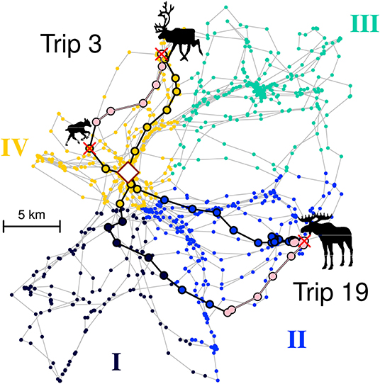
Figure 2. Illustration of two trips (#3 and #19) for wolf Niki superimposed on a four zone classification. Colored dots represent all locations collected for Niki over the two month period of the study. The four colors represent Zones I to IV as labeled along the exterior. In Trip 3, the wolf departed within Zone IV, killed a reindeer calf, moved along its boundary (pink colors), killed an adult reindeer, and returned to the den, entirely within Zone IV. In Trip 19, the wolf departed within Zone II, killed an adult moose at the boundary, moved along the boundary and returned via Zone I. Regardless of the return Zone, this trip is classified as a Zone II trip, since that is the direction chosen by the wolf at departure. The rhombus in the middle indicates the den site.
Whatever the eventual outcome of the trip (i.e., which zones the wolf visited, whether, where and how many prey are killed, etc.) the selected zone is a free and unconstrained choice that the wolf makes when it departs. The central assumption of our memory-based model is that choice of zone is driven, in part, by prior experiences—specifically, predation success and boundary visits—that are specific to each zone.
We model the selected zone for each trip (denoted Zt where t∈1, 2, ...nt) using a discrete choice modeling framework fitted with multinomial conditional logistic regression (Chapman and Staelin, 1982; Croissant, 2013). Discrete choice models are behavioral models designed to forecast the behavior of individuals facing a choice with unknown or unobservable estimates of utility of respective choices. They have been widely applied mainly to model human behavior, e.g., in behavioral economics (Louviere et al., 2000; McFadden, 2001; Dubé et al., 2002), including modeling transportation (Antonini et al., 2006) and food (Gracia and de Magistris, 2008; Czine et al., 2020) choices. In wildlife ecology, discrete choice models have been applied in the context of habitat selection, including in hierarchical frameworks across multiple individuals (Cooper and Millspaugh, 1999; McDonald et al., 2006; Thomas et al., 2006).
Discrete choice modeling allows for the statistical estimation of a ranking of choices where each choice can have a dynamic set of covariates. The model assumes that the wolf maintains a preference (or “desirability” or “priority”) score (Uit) for the ith zone at the time of trip t, and always chooses to head in the direction with the highest score. The preference score is separated into a systematic component (Vit) and unobserved component (ϵit):
It is important to note that the actual choice Uit may in fact be deterministic from the wolf's perspective, and neither the systematic nor the random component can be directly observed, as they represent the decision making process. But the partitioning allows us to analyze the process statistically. The deterministic portion is further decomposed into trip-specific and zone-specific component:
The coefficients βi are the zone-specific intercepts, reflecting the time-independent quality or preference of the particular zone. The trip-dependent set of variables Xit captures the dynamic scoring of the zones and the set of coefficients γv reflects the overall intrinsic response to each of the variables (indexed by v).
In our most complex model, we include three variables in Xit: a predation quality score (Xit1 = Pit), which tracks the zone-specific hunting success based on the wolf's experience, a boundary coverage score (Xit2 = Bit), which tracks whether a zone's boundary has been visited and, presumably, marked, and a repetition score (Xit3 = Rit) which tracks simply whether an animal went to a particular zone on the previous trip. The impact of these variables are driven by the wolf's memory and depend on several parameters as explained in detail below. The coefficients β and γ capture the relative contribution of each of environmental and experiential (cognitive) covariates. In total there are k+2 parameters in the most complex fitted model, one each for predation memory, boundary memory and repetition, and k−1 intercept parameters for each zone, minus one degree of freedom as the sum of the probabilities is always fixed to 1.
We assume the wolf tracks a zone-specific predation score, which is higher in areas with greater and more recent predation success, and a boundary score, which is higher in zones with more recent boundary visits. It is important to note that these scores (which are all positive) only quantify predation success and boundary visits, without making any claims as to whether higher values make directed departures more or less likely. Whether higher or lower scored areas are preferred is indicated by the strength and sign of the coefficient estimates of discrete choice model detailed in the next section. In fact, given the complexity of wolf and prey behavior, it is difficult to know a priori whether areas with a higher or lower number of kills would be preferred or avoided. Large prey items (e.g., adult moose or reindeer) are often cached, i.e., unconsumed portions are buried in the ground and returned to later (Peterson and Ciucci, 2003), which can make a recent kill site attractive. Similarly, the general suitability of a particular area for certain prey species can make areas of high predation success sequentially attractive. Prey behavior can further complicate these responses, as prey may also avoid areas with recent kills generating a “landscape of fear” (Laundré et al., 2010), and it may be more strategic to temporarily avoid a recently successful site.
Each kill contributes individually to the predation score corresponding to the zone of the kill. We assume that the score is higher the greater the mass of the kill, the shorter the time to the kill (i.e., the less the effort), and the more recent the kill. An expression that combines all of these assumptions is:
where the sum is performed over all of the prey items captured in zone i up to trip t (preyi, t); M is the approximate mass of the prey item; α ∈ [0, 1] is a mass-scaling parameter (details below); the effort Ej is the time spent moving before each kill either after leaving the den, or events that “pause” the hunting behavior, including cache revisits, or bedding; Δpj is the time since the predation event; τp is a memory time scale which captures how long the wolf considers previous successes valid or actionable; and κ is a memory discounting coefficient. Estimates for adult mass and estimated linear growth rates for the calves of the main ungulate prey (moose, forest, and semi-domesticated reindeer) were obtained from the literature as well as approximate mass of smaller mammals and birds (Table 1). Growth rates were, in particular, important to capture the growth of reindeer and moose calves, which are many times larger in late July than in the beginning of June.
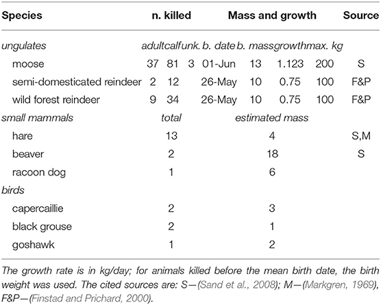
Table 1. Prey species, numbers killed, and growth models or estimated used to approximate mass obtained from each prey item in the predation module of the cognition model.
The form of this predation score reflects several strong structural assumptions, which we tested to a limited extent. For example, we set κ to be either 1 for exponential memory decay, or 2 for Gaussian decay. We also fitted models where the predation score did not include the discounting for effort, i.e., where Ej was always set equal to 1. This allowed us to test, in a narrow way, whether effort was also tracked. In both cases, fitted discrete choice models with the two different values of κ and with and without the effort term were compared using likelihood ratios.
The two free parameters for the predation memory module are the prey mass parameter α and the predation memory time scale τp. If α = 0, any prey item (whether a hare or an adult moose) contributes equally to the score. If α = 1, the contribution is proportional to mass. The memory coefficient τp captures the time scale at which memory is retained: if τp = ∞, all predation experience accumulates with no discounting for time.
The boundary memory attempts to track whether the wolf has patrolled and marked its boundary, an important behavioral goal. To algorithmically classify locations as boundary locations, we developed a concave hull algorithm that works as follows: (1) select the convex hull (i.e., vertices of the minimum convex polygon) Zmcp, (2) compute the angle θinner between all of the inner points Zinner and the respective pair of closest convex hull points, (3) retain the subset where , where θ* is a threshold of concavity, (4) repeat these steps using the combined set of Zmcp and as an input, (5) stop the iteration when the new set is identical to the input set. We used a threshold angle of θ* = π/2 (90°). This algorithm generated territorial boundary sets that were consistent with field determined boundary locations (see Figure A.1 for an example of the algorithm and Figure A.2 for all boundaries in Appendix A).
The boundary memory, denoted Bi, t is a binary (0, 1) variable that tracks whether the wolf has visited at least two locations on the boundary of zone i in a fixed time period λ preceding each trip. The λ parameter captures the interval of time that the wolf feels it is necessary to re-mark the territory and, therefore, related to the time a scent-marking fades. We anticipated that the choice regression coefficient for the boundary would be negative, indicating that a zone with a recently visited boundary will be scored lower.
Finally, we added a repetition variable Ri, t, which is simply 1 if the selected zone at trip t−1 was also i and 0 otherwise. This variable is included in the model to account for any serial auto-correlation (or anti-correlation) in the wolf's zone choice, which could be confounded with either of the predation or boundary variables.
Under the generic assumptions of independent and identical Gumbel distributions for the unobserved terms εit in Equation (1), the probabilities can be written in terms of the logit probability function:
and the coefficients can be estimated by full-information maximum likelihood estimation, as implemented in the mlogit package in R (Croissant, 2013).
The likelihood procedure provides estimates of the regression-like choice coefficients β (zone-specific estimates) and γ (contribution of predation, boundary memory, and repetition). However, the memory parameters (τp, λ, memory type κ) and the structural parameters (number of zones k) have to be assessed separately. Likelihood based criteria are useful for comparing models with different values of the memory coefficients; however, because the number of zones fundamentally alters the underlying data, likelihoods cannot be used to compare different fitted models across different numbers of zones. We, therefore, introduce an intuitive measure of predictive power of the models to use a basis of comparisons: the relative predictive improvement index (RPI) defined as the ratio of the mean of the predicted probabilities over the mean of the null probabilities, i.e.:
where the sums are across all trips t∈1, 2, ..., nt, and the null probabilities are the proportion of trips for each zone (note, since both sums are over the same number of trips, the ratio of the sums is equal to the ratio of the respective means). As an example, if an entire dataset consisted of one visit to each of 4 zones: z = (1, 2, 3, 4), and the model predictions for choosing each of those trips were Prt = (0.75, 0.5, 0.25, 0.5), then . The mean of the null probabilities is and the ratio of the two is RPI = 2, which can be interpreted as a doubling of the predictive power of the model. Note that model log-likelihoods and RPI are monotonically related: the former is the sum of the log of probabilities, while the latter is proportional to the sum of the probabilities. Thus a “maximum RPI” point estimate is equivalent to a maximum likelihood point estimate, though without the convenience of asymptotic theory for estimating confidence intervals on coefficients. However, a randomization test of the null hypothesis (that the model provides no improvement, i.e., RPI = 1) can be conducted by resampling the order of the trips some large number of times from the null set of probabilities, recalculating the RPI, and comparing the observed RPI to the resulting null distribution. Similarly, a resampling confidence interval can be obtained by sampling sequences of trip zones from the predicted probabilities of the model, and comparing to a sampling of zone sequences from the null model. By computing the RPI of these resamplings and repeating the process some large number of times (e.g., 1,000), a confidence interval can be obtained around the RPI. The RPI thus provides an intuitive, interpretable tool for assessing discrete choice models where the number of choices itself is variable, as well as a statistical mechanism for hypothesis testing and inference.
We fitted the discretized trip-choice data across a range of 3 to 8 zones, with predation time scales τp ranging from 0.5 to 4 (interval 0.25), boundary marking lags λ from 0.5 to 12 days (interval 0.5), for each of κ = 1 (exponential memory) and κ = 2 (Gaussian memory), for each of 8 summer movement data sets. We computed the RPI, and selected the combination of these parameters for which the RPI was maximized. The theoretical total number of fitted models was 45,360, but in many cases—usually those with a high number of zones of which some are never selected—the fits did not converge. In other cases, there are no evident maxima in the RPI. Nonetheless, from this set of models, we can pick out the best combination of selected parameters (k, τp and λ) for each wolf. Once those were determined, we compared eight models with every combination of explanatory variables (predation memory P, boundary memory B, or repetition R; i.e., P+B+R, P+B, P+R, B+R, P, B, R, Null) using AIC as a model selection criterion. From the final selected model, we report the estimates, confidence intervals and p-values of the retained coefficients.
As an added analysis, we compared estimates of the boundary and predation coefficients across respective memory time-scales to see if a particular response shifted across scales. A transition from, e.g., a positive to a negative response across time-scales would indirectly suggests that the memory driven response to a particular zone operates in different ways at different time-scales. In performing this analysis, we selected the best model and combination of structural parameters, i.e., number of zones and combination of covariates.
All symbols and definitions for the modeling, data preparation, and model assessment are presented in Table 2.
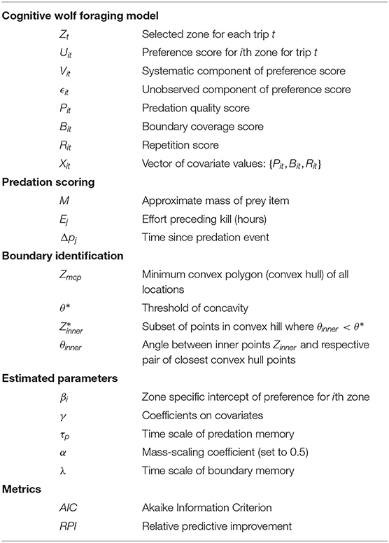
Table 2. Definitions and symbols for modeling, data preparation and model assessment.
Pack size varied considerably, which in turn meant the number and composition of prey killed varied by pack (Figure 3). The overwhelming majority of prey consumed was cervids (176 of 206 identified carcasses: 85%): 80 (39%) moose calves and 46 (22%) were reindeer calves, another 36 (17%) were adult moose and 11 (5%) were adult reindeer. The remaining prey items were all minor, mainly hare. The two largest, most established packs, on which we reported on in previous work (Gurarie et al., 2011), consumed by far the most prey (over 45 items each, compared to 22 for the next highest, Figure 3), which can partially be explained by their consumption of larger prey which was easier to locate in the field. Over the respective 60 day periods of field tracking, the number of trips greater than 2 h varied between 34 and 67 (mean 53, s.d. 12).
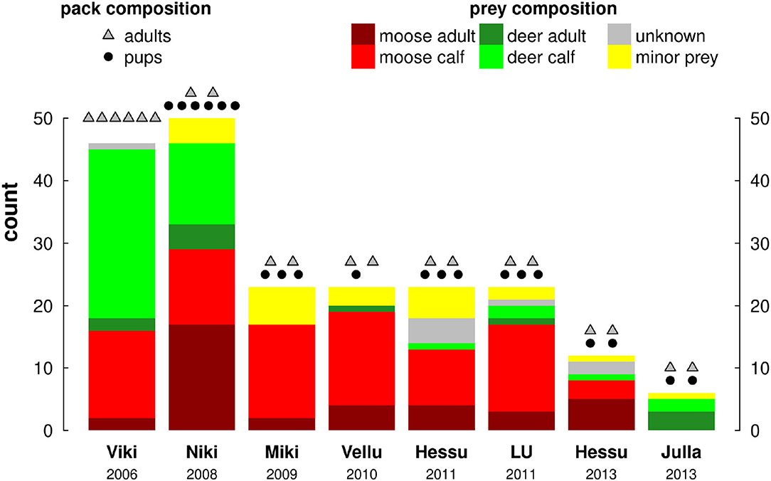
Figure 3. Pack and prey composition of all 8 pack-year studies, arranged chronologically by year. Colors indicate prey composition as per the legend, dots and triangles above the bars indicate the number of adults and pups in each pack, respectively.
While there are many structural parameters in the full cognitive model, the main ones of interest were those related to time scales of memory for predation and boundary visits, and spatial scales as reflected in the number of zones. We did, however, have to make decisions regarding several other parameters.
Thus, we initially explored two values of the memory decay shape parameter [κ in Equation (3)]: κ = 1 corresponding to an exponential memory decay, and κ = 2 corresponding to a Gaussian memory decay. We also explored two values of the mass scaling parameter α: α = 0.5—i.e., a square root scaling, and α = 1, a linear scaling. We fitted the complete (predation + boundary visit + repetition) discrete choice model over a range of scaling parameter values and each of the four combinations of α and κ and compared the likelihoods of fitted models. Results are summarized and presented in Appendix B.
There was high variability among individual animals when these models were fitted (see results in Appendix B). Some (e.g., Viki 2006) had a much higher likelihood with Gaussian decay and square root scaling, while for others (e.g., Niki 2008), the exact inverse was the case. The absolute differences in the log-likelihoods were not—typically—much larger than one, suggesting that the process was not sensitive to either of these parameters. We, therefore, chose to fix the “Viki” pattern (Gaussian decay and square root scaling) for all subsequent results, noting that those discrepancies may be worth further investigation. Subsequent analyses focused on the time scales of predation and boundary memory, and the spatial scales as defined by number of zones.
Similarly, we assessed the structural assumption that the effort component [Ej in Equation (3)] contributed significantly to the predation score as a predictor by comparing likelihoods of fits with and without the effort component across a range of parameter values. Again, there was considerable variability among individuals (see Appendix C), but for those four studies for which the effort model was a better model (Viki 2006, Niki 2008, Lentuan Uros 2011 and Julla 2013), the difference was rather large (most ΔAIC values < -2). These four wolves are also the four wolves for which predation was retained in the final discrete choice model (see below and Table 4). A broad preliminary conclusion is that hunting effort is indeed tracked by the wolf, and the “predation score” is tempered by longer effort times. We retained the effort term for all subsequent analyses.
We illustrate fits of the complete (P+B+R) cognitive model for one wolf, Lentuan Uros (LU 2011), across a range of zone breakdowns (Figure 4, upper panels) and values of boundary time lag λ and predation memory time scale τp (Figure 4, lower panels). We obtained over a 50% improvement on null predictions for this wolf (the highest of any of the other wolves), with RPI maxima ranging between 1.51 and 1.54 for spatial break-up into 5 to 8 zones. The RPI profile across boundary time scales is fairly consistent across number of zones, around 4.5 days, with the most prominent peak at 5 and 6 zones. The RPI profile against predation memory time scale peaks consistently between 1.25–1.75 days, though differences across time scales were less dramatic. Interestingly—the RPI-predation profile was sharper at the higher breakdown of zones (7 and 8) where the profile for boundary memory was flatter.
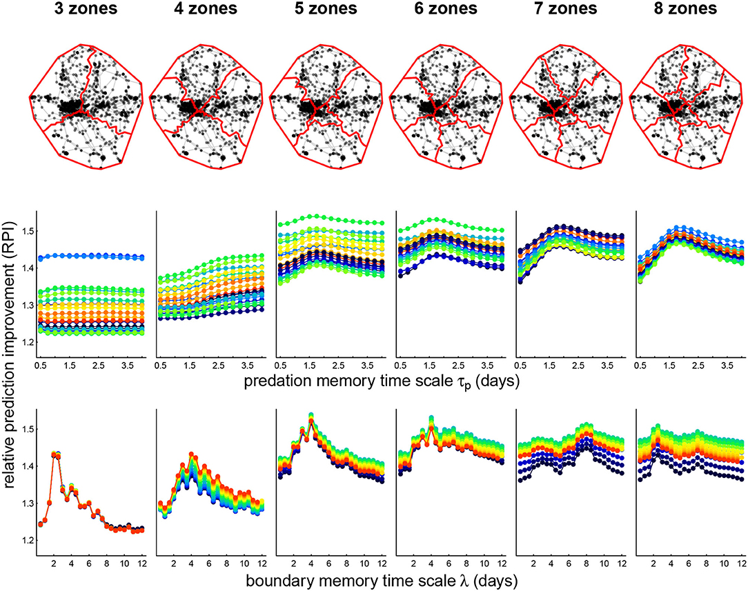
Figure 4. Zone breakdown (upper panels) and parameter sweep of memory models (lower panels) for wolf Lentuan Uros (LU). Upper panels illustrate the roughly axial separation that the zone clustering algorithm generated. Lower panels illustrate the computed prediction improvement (RPI) for predation and boundary fitted models across various values of predation memory time scale τp (middle panels) and boundary visit lags λ (lower panels). The color spectra correspond to the other time scale in each plot. Thus, for example, the maximum RPI (1.54) is attained at 5 zones, τp = 1.75 days and λ = 4 days.
At the highest RPI set of parameters (5 zones, τp = 1.75, λ = 4.0), a model comparison against all linear combinations of P, B, and R models show that there is essentially no difference between the P+B+R and B+R model, but that both of these are much better than any of the other models (ΔAIC > 4), and the null model performs much worse than any of the others (Table 3). The coefficients for boundary and repetition were both highly significant and positive, suggesting that the wolf tended to repeat its previous behavior, and, unexpectedly, that visits to boundary locations were further reinforced by recent visits, rather than recent visits obviating the need to return to a boundary.
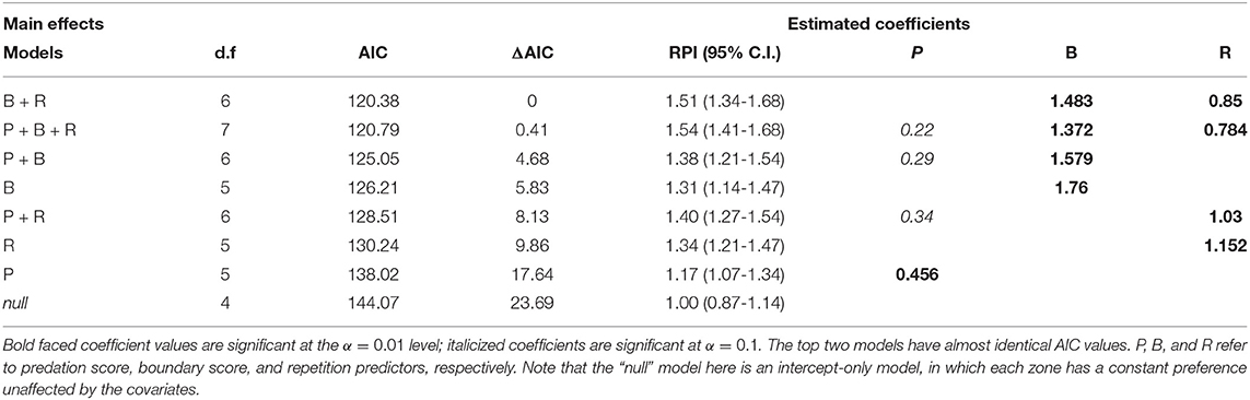
Table 3. ΔAIC table for comparison of fitted cognitive choice models for wolf LU 2011 with 5 zones, τp = 1.75, λ = 4.0, sorted by decreasing AIC, with d.f. representing the degrees of freedom (number of parameters).
A cognitive model improved significantly on the null RPI for six of the eight wolf studies at the best (or near best) combination of parameters (Table 4). We refer to these six studies as “cognitive wolves.” There was, however, considerable variability in the values of the RPI-maximizing parameters and in the signs of the fitted coefficients.
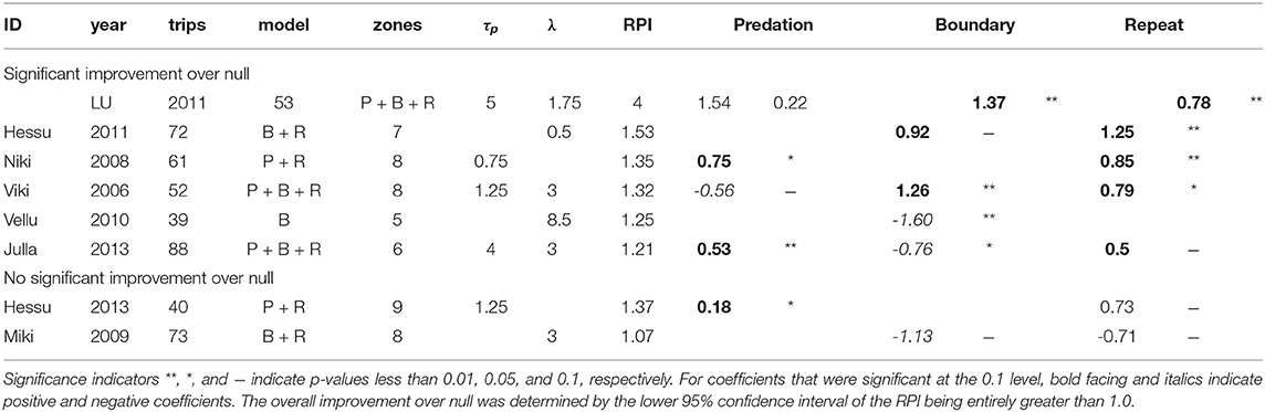
Table 4. Summary of model results for best (or near-best) model for each study, with selected parameter values, selected model, and coefficient estimates.
The repetition effect was positive and significant in all but one of the cognitive wolves, suggesting that wolves have some straightforward auto-correlation in their choice of departure direction. For three of the four cognitive wolves for whom the predation coefficient was retained, the effect was significant and positive—consistent with our a priori hypothesis that there would be a preference for zones with higher predation scores, consistent with the foraging site fidelity hypothesis. The exception was Viki 2006, who showed a negative response to predation at a memory time scale of 0.75 days. Similarly, the boundary effect was retained for five studies, of which three showed positive responses, while two showed negative responses. Vellu 2010, the only cognitive wolf for which repetition was non-significant, had a strongly negative boundary coefficient (at a lag of 8.5 days), indicating that boundary patrolling was a significant driver for this wolf, which also had the most elongated of all the territories (Figure 1). The only wolf that conformed with both of our hypothesized predictions was Julla 2013, with both a positive response to predation and a negative response to boundary visits.
We explored how the estimated effect sizes and signs changed across time scales of memory for boundary visits (λ from 1 to 20 days) and predation scores (τp from 0.5 to 5 days) for those wolves for which both were significant predictors of departure directions. Figure 5 illustrates three such examples.
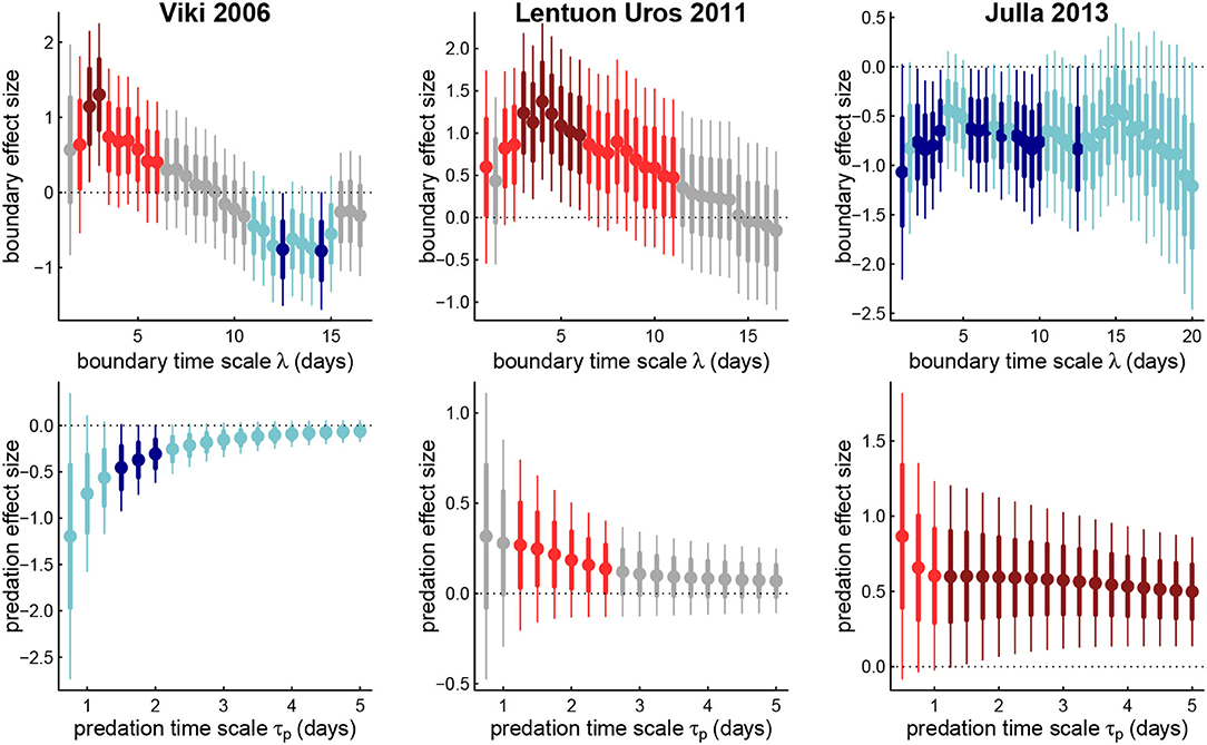
Figure 5. Estimated coefficients for boundary effects against boundary memory time scales (upper panels) and predation effect against predation memory timescale (lower panels) for three example wolves. Thick and thin bars represent 1 and 2 standard errors around respective point estimates, blue are negative, red are positive, light and dark colors represent 1 and 2 standard errors away from 0. Note that the boundary coefficient for Viki (left panels) switches signs across memory time scales.
Generally, for both predation and boundary visits, at the longest time scales, the less important is the memory for predicting intrisic values of areas, or at least at predicting the direction of foraging. However, unique patterns do emerge for each individual. Thus, Julla 2013 had a fairly consistent positive predation response (mean effect size 0.58), and negative boundary response (mean -0.72), more or less consistently across all time scales. For wolf LU, the positive boundary response peaks in magnitude around the value corresponding to the highest likelihood, around 4 days (Table 4), and then steadily decays until it ceases to be significant after about a value of λ = 10 d. The predation response decays steadily with greater time scale, becoming statistically insignificant after about 3 days.
Most strikingly, wolf Viki 2006 undergoes a switch in the sign of the boundary coefficient between short time lags (≈ 3 days) and longer time lags (≈ 12 days). This suggests that the wolf is more likely to revisit (or highly value) an area of recent visitation, but if the score considers whether there have been visits over a two week period, that area is less likely to be selected. This result is somewhat consistent with the short and long time-scaled memory, often referred to as “working” and “reference” which has been both experimentally measured (Green and Stanton, 1989; Becker and Morris, 1999) and modeled (Bracis et al., 2015, 2018). Recent visits to portions of a boundary may require more visits for good marking. But if a boundary has been marked over a larger time scale, while others have not been, then the need to go to unmarked areas increases. The strength of the predation response for Viki 2006 is significantly negative at a 1.5–2 day time scale, indicating that more or less immediate returns to areas with successful kills are unlikely. However, as that predation memory time scale increases, recent predation success becomes less significant as a predictor of future movements.
Cognitive processes cannot be directly observed for animals in the wild; even in controlled experiments memory can only be inferred. Studying cognition, therefore, requires developing a cognitive model to make inferences on those behavioral observations, like movements and predation events, that are the observable outcomes of cognitive processes. In order to demonstrate that central-place foraging wolves are using memory to make movement decisions, we needed several specific ingredients: (1) a discrete, observable set of choices made by wolves in the wild, (2) significant events (kills and boundary visits) that could reasonably have influenced the valuing of those choices, (3) a statistical framework that allowed for a rapid exploration of various temporal and spatial scales at which memory might operate, combined with a model selection framework to narrow down significant explanatory variables, and (4) a metric by which we could demonstrate that our model outperforms a non-cognitive model. For most wolves, fitted and parameterized cognitive models were 20 to 50% better at predicting choices than non-cognitive null models (Table 4).
In order to develop and fit such models, we relied on an extraordinarily detailed dataset which contained reliable information on objects and locations that are known to be of importance to wolves during the breeding season: the precise location of the den, of kill sites with identification of prey species, and—with slightly more guesswork—the contours of the territorial boundary. We therefore constructed our model around the behavioral imperatives of predation and territorial marking, anchored around fairly regular, central-placed trips that began and ended at the den site. The model assumed a spatially-explicit scoring that emerges directly from prior experiences for both priorities. These are generic assumptions that are consistent with well-known aspects of wolf behavior (Mech and Boitani, 2003).
Nonetheless—and most intriguingly—the results we obtained in many cases contradicted our expectations and were highly individual and idiosyncratic. We comment here on the design and structure of our modeling framework, discuss the cognitive spatial ecology of the wolves in our study, and conclude with some broad ideas on the ingredients needed to make cognitive inferences on animals in the wild.
We chose a discrete choice framework with a design that focused on the apparently unconstrained choice of direction taken by the wolf when leaving the den. The discrete choice approach is a natural one for exploring cognition for several reasons. First, experimental studies of memory and learning in animals almost always reduce to discrete choice frameworks (Thorpe et al., 2004), including such classic experimental designs as the turns a rat chooses to navigate a maze (Tolman and Honzik, 1930) or key-pecking by pigeons (Wilkie and Willson, 1992). More relevant to wolves, experiments on domestic dogs Canis familiaris that have shown explicit episodic and working memory have been designed around hiding food rewards in discrete boxes (Fiset et al., 2003; Fujita et al., 2012). Second, the statistical analysis of observational data on discrete choices is a well-developed field, in particular as related to human economic choices (Louviere et al., 2000; McFadden, 2001; Dubé et al., 2002). Fitting discrete choice models is, therefore, fast and technically straightforward, and provides easily interpretable effect sizes for any number of statistically supported covariates that might independently influence choices. Finally, a discrete choice framework provides a straightforward measure of the predictive success of models by comparing probabilistic predictions to randomized observations.
Despite the natural fit of the discrete choice framework to studying cognition, this study is the only example we are aware of as applied to a free-ranging wild animal. The key ingredient is the discrete choice itself. We focused on a very specific kind of movement: namely the early stage of departure from a den. Given the high motility of wolves and the relatively unstructured Finnish mixed woodland landscape, any destination was more or less equally available. Furthermore, it seemed a safe assumption that each departure from the den had similar essential purposes: first to obtain food by hunting or visiting existing caches, with the goal of returning with enough nourishment to feed pups in the den, and to patrol territories. By reducing our movement variable in this way, we greatly simplified the general problem of “modeling movements.” This is in contrast to a thematically similar study, in which a memory-based model of winter (i.e., non den-centric) wolf movements with boundary visits and prey habitat used as covariates (Schlägel et al., 2017). In their compelling analysis, every movement step was modeled and the spatial map was fixed to a computationally feasible grid. Thus, the spatial and temporal units of analysis were set not by biological or behavioral considerations but by the battery power trade-off of collar transmission, and by computational constraints of spatial grid processing. The intensive computation of fitting a single model (several days, Schlägel, pers. comm.) limited the ability to explore different parameterizations, model structures or covariates. Furthermore, the nature of movements can vary considerably depending on the motivation or behavioral imperative. For example, previous work on several of the wolves in this study showed that movements are faster and more directed when returning to a den post-kill than while hunting (Gurarie et al., 2011), a distinction that is lost when all movements are assumed to be driven by the same process.
By focusing on a limited set of discrete trip departures and a coarsely discretized spatial structure, we were able to compare thousands of models in a short amount of time, sweeping across multiple temporal and spatial scales and combinations of structural parameter values. The obvious trade-off is that we had relatively few departures to model, no more than 1 per day per wolf, which limited the inferential power of more complex models.
Among the many structural assumptions underlying our framework, perhaps the most tenuous was the discretization of the wolf territories into a countable number of zones. There is no objective way to know how similar a wolf's mental map might be to our clustering-based zonal partitioning. However, we were able to test a range of numbers of zones, from 3—too few to provide interesting insights—to 8—at the limit of discrete choices given the number of trips that we analyze per wolf. By comparing these different spatial structures, we were able to obtain a coarse idea of a spatial scale at which wolves might be conceptualizing their territory. The number of zones that best separated the discrete choice making of the wolves was between 5 and 8, i.e., in the upper half of the range. Noting that the mean area of the wolf territory was around 670 km2 (s.d. 275), this would suggest that a relevant cognitive spatial scale for valuing areas would be on the order of 80–130 km2. Note that this sweeping of structural parameters is made tractable, even trivial, by the discrete choice model framework.
For the animals for which predation memory was significant, three were between 0.75 and 1.75 days (Table 4), which might be considered an indication of the time frame over which the spatial location of a predation success is relevant to a wolf. Larger prey items were often torn into smaller pieces and cached, i.e., buried shallowly, by the wolves. Those caches are often revisited within some relatively short period after the kill before any useful meat is too spoiled, and the 1–2 day time scale might reflect that specific cache-revisit behavior. For those wolves for which boundary visits were a significant factor, time-scales were nearly all much longer: from 3 to 8.5 days (Table 4).
The shift in the magnitude of the coefficient responses (Figure 5) adds nuance to this discussion of time scales. Most notably, the shift in the sign of the boundary response against time scales for wolf Viki is somewhat consistent with the paradigm of “working” (short-term) and “reference” (long-term) memories that often operate in different ways (with opposite signs) at different time-scales. Similarly, while we discretized space into relatively few large zones, in Figure 4 it appears that the RPI peak against predation time-scale is narrower at a larger number of zones (8), i.e., at a finer spatial scale, while RPI against boundary memory is more sharply optimized at fewer zones (5). This may indicate that the spatial scale at which predation success is remembered is finer than the spatial scale of boundary patrolling. This is consistent with the fact that predation occurs unpredictably in very specific locations, whereas the boundary is a known, fixed entity which is most efficiently marked by making larger territorial movements. Including multiple temporal and spatial scales in a model like this, however, stretches the power of limited observations for making inferences.
While the fitting, parameterization and predictive assessment of the cognitive model was largely successful, many of the estimated effects contradicted our original expectations and point to nuanced and context-dependent strategies of foraging. In particular, we anticipated that the predation memory effect would be positive, corresponding to a strategy of foraging-site fidelity, and that the boundary visit effect would be negative, as recently visited boundaries would not need to be revisited immediately.
In fact, only one wolf (Julla) has a significant positive predation memory at a time scale of 4 days (by far the longest time scale) combined with a significant negative boundary memory (time scale 3 days). Julla was a wolf in a small pack (2 adults) which apparently only killed 5 reindeer (of which three were adults) that were identified by field workers over the study period. With so few animals, caching and memory takes on an additionally important role, and likely contributed to the higher scoring of recent predation kill sites. Apparent foraging site fidelity in this context is possibly more closely related to cache returns than persistent prey density.
Julla can be contrasted to another wolf (Viki) that had a weak (0.1 > p-value > 0.5) negative coefficient on the predation memory (time scale of 1.25 days). Viki apparently did not value locations of recent predation success as highly as moving to other areas of its territory. Viki was a reproductive member of the largest, most established pack in our data set in the core Finnish wolf area, and had among the largest number of kills, 44 reindeer and moose, mainly calves, in total (Figure 3). It is possible that the high success rate of predation throughout the range, together with the higher need to patrol boundaries, and reinforcing territorial marking, deemphasizes the need for foraging site fidelity. Furthermore, it is possible that local prey depletion can occur, analogous to the “patch-disturbance” hypothesis that leads lions to regularly change the location they predate after successful hunts due to prey species avoiding environments that are demonstrably risky (Valeix et al., 2011). While the viewshed and corresponding cross-prey species communication of successful hunts is much more limited in the boreal forest than in the savanna, many of the prey ungulates have much smaller ranges than the smallest of the wolf zones. For example, summer home ranges of female moose in Fennoscandia range from 1000 to 2000 ha (Cederlund and Okarma, 1988; Eriksen et al., 2011). Moose are, furthermore, solitary and somewhat territorial, with minimal range overlap (Eriksen et al., 2011). A single adult kill may, therefore, significantly deplete the availability of prey on a hyper-local level, while a calf kill—which a mother moose is likely to be aware of—may also result in a shift in the female's range.
In contrast to both Viki and Julla, Niki had a strong positive predation coefficient (at time lag 0.75), and no boundary model selected whatsoever, despite having the greatest number of kills. This may be explained by the fact that Niki's territory was largely structured by several major roads and an extended fence separating the reindeer management area (RMA, Figure 1). In fact, Niki was the only wolf whose territory overlapped with the RMA and the only wolf to have killed several semi-domesticated reindeer (Gurarie et al., 2011). All of these highly structuring features are consistent with certain areas being consistently better for predation, making foraging site fidelity a more viable strategy for this wolf.
While accounting for the wide variability in cognitive strategies among these wolves is impossible, we can broadly conclude that wolves may engage in either major foraging strategy, or—indeed—can move with no particular attention to prey distribution at all. It bears noting that the territories in this study were all very similar, many neighboring or overlapping across years (Figure 1). The main differences among wolves were related to pack composition and density and distribution of primary roads and houses, which can significantly impact wolf behavior and space use in general (Gurarie et al., 2011; Barry et al., 2020). Thus, when it comes to using and responding to spatial memory, wolves appear to be highly idiosyncratic and individual, much as the social and ecological context of individual wolves can be very specific, even within the same territory across years (see also Appendix B). Even as it can be demonstrated statistically that some decisions are influenced by prior experience, there are few overarching generalities that can be made about the spatial or temporal scales and relative importance of various cues on wolf cognition.
It is—in short—a surprisingly steep challenge to infer the use of memory for animals moving in the wild, mainly because of the large number of variables that cannot be controlled and the complexity of animal behavior. Nonetheless, cognitive inferences can be made when certain criterion are met. We propose here a checklist building on the somewhat qualified success of fitting our own cognitive model on the wolf data set.
1. Identification and isolation of a distinct quantifiable behavior that might hypothetically be driven by prior experiences and otherwise be minimally confounded by unknown behavioral imperatives; e.g., den departures to specific spatial zones.
2. Identification of key events or cues that might determine the movement behavior to be modeled; in our example, predation events and boundary visits. Generally, food resources are the most important trigger, echoing experimental setups where food rewards are routinely used. As a rule, movement data alone without a context will almost never be sufficient to unambiguously identify a cognitive signal.
3. A plausible cognitive mechanism for a movement response to those events; i.e., the memory-based movement model itself. Ideally, this model can be developed in a hierarchical way, such that increasingly complex models can be compared to test specific hypotheses.
4. A statistical framework to estimate the properties of that mechanism from movement data; e.g., the discrete choice modeling framework and parameter sweeps for maximum likelihood exploration of parameter values.
5. A reliable metric to demonstrate the relative performance of the cognitive model against simpler, non-cognitive models; e.g., the relative prediction improvement score.
This checklist may be useful in pointing toward general principles for the development of cognitive analysis of movement data.
The raw data supporting the conclusions of this article will be made available by the authors, without undue reservation.
This research adheres to the ASAB/ABS Guidelines for the use of animals in research. The capture protocol of wolves in 2008–2013 followed conditions in permits approved by the Animal Experimental Board–ELLA, Southern Finland State Administrative Agency (licence numbers ESLH-2008-01012/Ym-23, ESLH-2008-10222/Ym-23, ESAVI-0000184/041003/2011, and ESAVI/3893/04.10.03/2011), to which the use of the permit is reported annually. The capture of wolves in 2006–2007 met the guidelines issued by the Animal Care and Use Committee at the University of Oulu (OYEKT-6–99), under permits provided by the provincial government of Oulu (OLH-01951/Ym-23). All protocols adhered to directives 86/609/EEC (2006–2012) and 2010/63/EU (2013–2017).
EG, OO, and IK formulated the original concept. IK and JS coordinated and collected wolf data (with some help from EG). EG, WF, and CB contributed to conceptual model development. AB and SP contributed to data processing and coding. SP contributed to supplementary figures. EG conducted the analyses and wrote the initial manuscript draft. All authors contributed to manuscript revisions and have read, and approved the submitted version.
The authors declare that the research was conducted in the absence of any commercial or financial relationships that could be construed as a potential conflict of interest.
All claims expressed in this article are solely those of the authors and do not necessarily represent those of their affiliated organizations, or those of the publisher, the editors and the reviewers. Any product that may be evaluated in this article, or claim that may be made by its manufacturer, is not guaranteed or endorsed by the publisher.
The authors are indebted to the many field workers and volunteers who contributed to collecting summer predation field data on all the wolf studies. NSF grant DBI1915347 to WF and EG further supported this research. OO was funded by Academy of Finland (grant no. 309581), Jane and Aatos Erkko Foundation, Research Council of Norway through its Centres of Excellence Funding Scheme (223257), and the European Research Council (ERC) under the European Union's Horizon 2020 research and innovation programme (grant agreement no 856506; ERC-synergy project LIFEPLAN).
The Supplementary Material for this article can be found online at: https://www.frontiersin.org/articles/10.3389/fevo.2022.768478/full#supplementary-material
Abrahms, B., Hazen, E. L., Aikens, E. O., Savoca, M. S., Goldbogen, J. A., Bograd, S. J., et al. (2019). Memory and resource tracking drive blue whale migrations. Proc. Natl. Acad. Sci. 116, 5582–5587. doi: 10.1073/pnas.1819031116
Alfredéen, A.-C.. (2006). Denning Behaviour and Movement Pattern During Summer of Wolves Canis Lupus on the Scandinavian Peninsula (Ph.D. thesis). Sveriges lantbruksuniversitet. Institutionen för naturvårdsbiologi.
Antonini, G., Bierlaire, M., and Weber, M. (2006). Discrete choice models of pedestrian walking behavior. Transp. Res. B Methodol. 40, 667–687. doi: 10.1016/j.trb.2005.09.006
Avgar, T., Baker, J. A., Brown, G. S., Hagens, J. S., Kittle, A. M., Mallon, E. E., et al. (2015). Space-use behaviour of woodland caribou based on a cognitive movement model. J. Animal Ecol. 84, 1059–1070. doi: 10.1111/1365-2656.12357
Avgar, T., Deardon, R., and Fryxell, J. M. (2013). An empirically parameterized individual based model of animal movement, perception, and memory. Ecol. Model. 251, 158–172.
Baddeley, A., Rubak, E., and Turner, R. (2015). Spatial Point Patterns: Methodology and Applications With R. (London: Chapman and Hall/CRC Press).
Barraquand, F., Inchausti, P., and Bretagnolle, V. (2009). Cognitive abilities of a central place forager interact with prey spatial aggregation in their effect on intake rate. Animal Behav. 78, 505–514. doi: 10.1016/j.anbehav.2009.06.008
Barry, T., Gurarie, E., Cheraghi, F., Kojola, I., and Fagan, W. F. (2020). Does dispersal make the heart grow bolder? avoidance of anthropogenic habitat elements across wolf life history. Animal Behav. 166, 219–231. doi: 10.1016/j.anbehav.2020.06.015
Becker J. T. and Morris, R. G.. (1999). Working memory(s). Brain Cogn. 41, 1–8. doi: 10.1006/brcg.1998.1092
Boyce, M., and McDonald, L. (1999). Relating populations to habitats using resource selection functions. Trends Ecol. Evol. 14, 268–272. doi: 10.1016/S0169-5347(99)01593-1
Bracis, C., Gurarie, E., Rutter, J. D., and Goodwin, R. A. (2018). Remembering the good and the bad: memory-based mediation of the food–safety trade-off in dynamic landscapes. Theor. Ecol. 11, 1–15. doi: 10.1007/s12080-018-0367-2
Bracis, C., Gurarie, E., Van Moorter, B., and Goodwin, R. A. (2015). Memory effects on movement behavior in animal foraging. PLoS ONE 10:e0136057. doi: 10.1371/journal.pone.0136057
Bracis, C., and Mueller, T. (2017). Memory, not just perception, plays an important role in terrestrial mammalian migration. Proc. R. Soc. B 284:20170449. doi: 10.1098/rspb.2017.0449
Carroll, G., Harcourt, R., Pitcher, B. J., Slip, D., and Jonsen, I. (2018). Recent prey capture experience and dynamic habitat quality mediate short-term foraging site fidelity in a seabird. Proc. R. Soc. B Biol. Sci. 285:20180788. doi: 10.1098/rspb.2018.0788
Cederlund, G. N., and Okarma, H. (1988). Home range and habitat use of adult female moose. J. Wildlife Manag. 52:336. doi: 10.2307/3801246
Chapman, R. G., and Staelin, R. (1982). Exploiting rank ordered choice set data within the stochastic utility model. J. Market. Res. 288–301. doi: 10.2307/3151563
Cooper, A. B., and Millspaugh, J. J. (1999). The application of discrete choice models to wildlife resource selection studies. Ecology 80, 566–575. doi: 10.1890/0012-9658(1999)080[0566:TAODCM]2.0.CO;2
Czine, P., Trk, Á., Pető, K., Horváth, P., and Balogh, P. (2020). The impact of the food labeling and other factors on consumer preferences using discrete choice modeling—the example of traditional pork sausage. Nutrients 12:1768. doi: 10.3390/nu12061768
Davoren, G. K., Montevecchi, W. A., and Anderson, J. T. (2003). Search strategies of a pursuit-diving marine bird and the persistence of prey patches. Ecol. Monographs 73, 463–481. doi: 10.1890/02-0208
Dubé, J.-P., Chintagunta, P., Petrin, A., Bronnenberg, B., Goettler, R., Seetharaman, P. B., et al. (2002). Structural applications of the discrete choice model. Market. Lett. 13, 207–220. doi: 10.1023/A:1020266620866
Eriksen, A., Wabakken, P., Zimmermann, B., Andreassen, H. P., Arnemo, J. M., Gundersen, H., et al. (2011). Activity patterns of predator and prey: a simultaneous study of GPS-collared wolves and moose. Animal Behav. 81, 423–431. doi: 10.1016/j.anbehav.2010.11.011
Fagan, W. F., Lewis, M. A., Auger-Mth, M., Avgar, T., Benhamou, S., Breed, G., et al. (2013). Spatial memory and animal movement. Ecol. Lett. 16, 1316–1329. doi: 10.1111/ele.12165
Finstad, G., and Prichard, A. (2000). Growth and body weight of free-range reindeer in western alaska. Rangifer 20, 221–227. doi: 10.7557/2.20.4.1517
Fiset, S., Beaulieu, C., and Landry, F. (2003). Duration of dog (Canis familiaris) working memory in search for disappearing objects. Animal Cogn. 6, 1–10. doi: 10.1007/s10071-002-0157-4
Forester, J., Ives, A., Turner, M., Anderson, D., Fortin, D., Beyer, H., et al. (2007). State-space models link elk movement patterns to landscape characteristics in yellowstone national park. Ecol. Monographs. 77, 285–299. doi: 10.1890/06-0534
Fujita, K., Morisaki, A., Takaoka, A., Maeda, T., and Hori, Y. (2012). Incidental memory in dogs (Canis familiaris): adaptive behavioral solution at an unexpected memory test. Animal Cogn. 15, 1055–1063. doi: 10.1007/s10071-012-0529-3
Fuller, T. K., and Sampson, B. A. (1988). Evaluation of a simulated howling survey for wolves. J. Wildlife Manag. 52:60. doi: 10.2307/3801059
Gracia, A., and de Magistris, T. (2008). The demand for organic foods in the south of italy: a discrete choice model. Food Policy 33, 386–396. doi: 10.1016/j.foodpol.2007.12.002
Green, R. J., and Stanton, M. E. (1989). Differential ontogeny of working memory and reference memory in the rat. Behav. Neurosci. 103, 98.
Gurarie, E., Bracis, C., Delgado, M., Meckley, T. D., Kojola, I., and Wagner, C. M. (2016). What is the animal doing? tools for exploring behavioural structure in animal movements. J. Animal Ecol. 85, 69–84. doi: 10.1111/1365-2656.12379
Gurarie, E., Suutarinen, J., Kojola, I., and Ovaskainen, O. (2011). Summer movements, predation and habitat use of wolves in human modified boreal forests. Oecologia 165, 891–903. doi: 10.1007/s00442-010-1883-y
Hebblewhite, M., Merrill, E., and McDonald, T. (2005). Spatial decomposition of predation risk using resource selection functions: an example in a wolf–elk predator–prey system. Oikos 111, 101–111. doi: 10.1111/j.0030-1299.2005.13858.x
Jalanka, H. H., and Roeken, B. O. (1990). The use of medetomidine, medetomidine-ketamine combinations, and atipamezole in nondomestic mammals: a review. J. Zoo Wildlife Med. 21, 259–282.
Jędrzejewski, W., Schmidt, K., Theuerkauf, J., Jędrzejewska, B., and Okarma, H. (2001). Daily movements and territory use by radio-collared wolves (Canis lupus) in Bialowieza Primeval Forest in Poland. Can. J. Zool. 79, 1993–2004. doi: 10.1139/z01-147
Kojola, I., Aspi, J., Hakala, A., Heikkinen, S., Ilmoni, C., and Ronkainen, S. (2006). Dispersal in an expanding wolf population in Finland. J. Mammal. 87, 281–286. doi: 10.1644/05-MAMM-A-061R2.1
Kojola, I., Huitu, O., Toppinen, K., Heikura, K., Heikkinen, S., and Ronkainen, S. (2004). Predation on European wild forest reindeer (Rangifer tarandus) by wolves (Canis lupus) in Finland. J. Zool. 263, 229–235. doi: 10.1017/S0952836904005084
Laundré, J. W., Hernández, L., and Ripple, W. J. (2010). The landscape of fear: ecological implications of being afraid. Open Ecol. J. 3, 1–7. doi: 10.2174/1874213001003030001
Louviere, J. J., Hensher, D. A., and Swait, J. D. (2000). Stated Choice Methods: Analysis and Applications. (Cambridge: Cambridge University Press).
McClintock, B., King, R., Thomas, L., Matthiopoulos, J., McConnell, B., and Morales, J. (2012). A general discrete-time modeling framework for animal movement using multistate random walks. Ecol. Monographs 82, 335–349. doi: 10.1890/11-0326.1
McDonald, T. L., Manly, B. F. J., Nielson, R. M., and Diller, L. V. (2006). Discrete-choice modeling in wildlife studies exemplified by northern spotted owl nighttime habitat selection. J. Wildlife Manag. 70, 375–383. doi: 10.1080/09640568.2021.1924124
Mech, L., and Boitani, L. (2003). “Chapter 1 - wolf social ecology,” in Wolves: Behaviour, Ecology, and Conservation, eds L. Mech, and L. Boitani (Chicago, IL: The University of Chigaco Press).
Merkle, J., Fortin, D., and Morales, J. M. (2014). A memory-based foraging tactic reveals an adaptive mechanism for restricted space use. Ecol. Lett. 17, 924–931. doi: 10.1111/ele.12294
Merkle, J. A., Potts, J. R., and Fortin, D. (2016). Energy benefits and emergent space use patterns of an empirically parameterized model of memory-based patch selection. Oikos 126:185196. doi: 10.1111/OIK.03356
Morales, J. M., Haydon, D. T., Frair, J., Holsinger, K. E., and Fryxell, J. M. (2004). Extracting more out of relocation data: building movement models as mixtures of random walks. Ecology. 85, 2436–2445. doi: 10.1890/03-0269
Mueller, T., and Fagan, W. F. (2008). Search and navigation in dynamic environments–from individual behaviors to population distributions. Oikos 117, 654–664. doi: 10.1111/j.0030-1299.2008.16291.x
Nathan, R., Getz, W. M., Revilla, E., Holyoak, M., Kadmon, R., Saltz, D., et al. (2008). A movement ecology paradigm for unifying organismal movement research. Proc. Natl. Acad. Sci. U.S.A. 105, 19052–19059. doi: 10.1073/pnas.0800375105
Oliveira-Santos, L. G. R., Forester, J. D., Piovezan, U., Tomas, W. M., and Fernandez, F. A. S. (2016). Incorporating animal spatial memory in step selection functions. J. Animal Ecol. 85, 516–524. doi: 10.1111/1365-2656.12485
Peters, R. P., and Mech, L. D. (1975). Scent-marking in wolves: radio-tracking of wolf packs has provided definite evidence that olfactory sign is used for territory maintenance and may serve for other forms of communication within the pack as well. Am. Scientist 63, 628–637.
Peterson, R. O., and Ciucci, P. (2003). “Chapter 4 - the wolf as a carnivore,” in Wolves: Behavior, Ecology, and Conservation, eds L. Mech, and L. Boitani (Chicago, IL: The University of Chigaco Press).
Riotte-Lambert, L., Benhamou, S., Bonenfant, C., and Chamaillé-Jammes, S. (2017). Spatial memory shapes density dependence in population dynamics. Proc. R. Soc. B Biol. Sci. 284:20171411. doi: 10.1098/rspb.2017.1411
Sand, H., Wabakken, P., Zimmermann, B., Johansson, O., Pedersen, H. C., and Liberg, O. (2008). Summer kill rates and predation pattern in a wolf-moose system: can we rely on winter estimates? Oecologia 156, 53–64. doi: 10.1007/s00442-008-0969-2
Schlägel, U. E., and Lewis, M. A. (2014). Detecting effects of spatial memory and dynamic information on animal movement decisions. Methods Ecol. Evol. 5, 1236–1246. doi: 10.1111/2041-210X.12284
Schlägel, U. E., Merrill, E. H., and Lewis, M. A. (2017). Territory surveillance and prey management: wolves keep track of space and time. Ecol. Evol. 7, 8388–8405. doi: 10.1002/ece3.3176
Thomas, D. L., Johnson, D., and Griffith, B. (2006). A bayesian random effects discrete-choice model for resource selection: population-level selection inference. J. Wildlife Manag. 70, 404–412. doi: 10.2193/0022-541X(2006)70[404:ABREDM]2.0.CO;2
Thorpe, C. M., Jacova, C., and Wilkie, D. M. (2004). Some pitfalls in measuring memory in animals. Neurosci. Biobehav. Rev. 28, 711–718. doi: 10.1016/j.neubiorev.2004.09.013
Thurfjell, H., Ciuti, S., and Boyce, M. S. (2014). Applications of step-selection functions in ecology and conservation. Movement Ecol. 2:4. doi: 10.1186/2051-3933-2-4
Tolman, E. C., and Honzik, C. H. (1930). “Introduction and removal of reward, and maze performance in rats,” in University of California Publications in Psychology. Berkeley, CA: University Press.
Valeix, M., Chamaillé-Jammes, S., Loveridge, A. J., Davidson, Z., Hunt, J. E., Madzikanda, H., and MacDonald, D. M. (2011). Understanding patch departure rules for large carnivores: lion movements support a patch-disturbance hypothesis. Am. Nat. 178, 269–275. doi: 10.1086/660824
Van Moorter, B., Visscher, D., Benhamou, S., Börger, L., Boyce, M. S., and Gaillard, J. M. (2009). Memory keeps you at home: a mechanistic model for home range emergence. Oikos. 118, 641–652. doi: 10.1111/j.1600-0706.2008.17003.x
Van Moorter, B., Visscher, D., Herfindal, I., Basille, M., and Mysterud, A. (2013). Inferring behavioural mechanisms in habitat selection studies getting the null-hypothesis right for functional and familiarity responses. Ecography 36, 323–330. doi: 10.1111/j.1600-0587.2012.07291.x
Watkins, K. S., and Rose, K. A. (2013). Evaluating the performance of individual-based animal movement models in novel environments. Ecol. Model. 250, 214–234. doi: 10.1016/j.ecolmodel.2012.11.011
Keywords: discrete choice modeling, wolf, movement, predation, boundary patrolling, central place foraging, foraging site fidelity, foraging site switching
Citation: Gurarie E, Bracis C, Brilliantova A, Kojola I, Suutarinen J, Ovaskainen O, Potluri S and Fagan WF (2022) Spatial Memory Drives Foraging Strategies of Wolves, but in Highly Individual Ways. Front. Ecol. Evol. 10:768478. doi: 10.3389/fevo.2022.768478
Received: 31 August 2021; Accepted: 27 January 2022;
Published: 14 March 2022.
Edited by:
Louise Riotte-Lambert, University of Glasgow, United KingdomReviewed by:
Marion Valeix, Centre National de la Recherche Scientifique (CNRS), FranceCopyright © 2022 Gurarie, Bracis, Brilliantova, Kojola, Suutarinen, Ovaskainen, Potluri and Fagan. This is an open-access article distributed under the terms of the Creative Commons Attribution License (CC BY). The use, distribution or reproduction in other forums is permitted, provided the original author(s) and the copyright owner(s) are credited and that the original publication in this journal is cited, in accordance with accepted academic practice. No use, distribution or reproduction is permitted which does not comply with these terms.
*Correspondence: Eliezer Gurarie, ZWd1cmFyaWVAZXNmLmVkdQ==
Disclaimer: All claims expressed in this article are solely those of the authors and do not necessarily represent those of their affiliated organizations, or those of the publisher, the editors and the reviewers. Any product that may be evaluated in this article or claim that may be made by its manufacturer is not guaranteed or endorsed by the publisher.
Research integrity at Frontiers
Learn more about the work of our research integrity team to safeguard the quality of each article we publish.