Individual Network Topology of Patch Selection Under Influence of Drifting Site Fidelity

Network theory has led to important insight into statistical-mechanical aspects of systems showing scaling complexity. I apply this approach to simulate the behavior of animal space use under the influence of memory and site fidelity. Based on the parsimonious Multi-scaled random walk model (MRW) an emergent property of self-reinforcing returns to a subset of historic locations shows how a network of nodes grows into an increased hierarchical depth of site fidelity. While most locations along a movement path may have a low revisit probability, habitat selection is maturing with respect to utilization of the most visited patches, in particular for patches that emerge during the early phase of node development. Using simulations with default MRW properties, which have been shown to produce space use in close statistical compliance with utilization distributions of many species of mammals, I illustrate how a shifting spatio-temporal mosaic of habitat utilization may be described statistically and given behavioral-ecological interpretation. The proposed method is illustrated with a pilot study using black bear Ursus americanus telemetry fixes. One specific parameter, the Characteristic Scale of Space Use, is here shown to express strong resilience against shifting site fidelity. This robust result may seem counter-intuitive, but is logical under the premise of the MRW model and its relationship to site fidelity, whether stable or shifting spatially over time. Thus, spatial analysis of the dynamics of a gradually drifting site fidelity using simulated scenarios may indirectly cast light on the dynamics of movement behavior as preferred patches are shifting over time. Both aspects of complex space use, network topology and dynamically drifting dispersion of site fidelity, provide in tandem important descriptors of behavioral ecology with relevance to habitat selection.

Introduction

Animals’ cognitive capacity to utilize a memory map in their quest for optimizing habitat selection continues to be verified empirically from data on vertebrate movement, including amphibians (Pasukonis et al., 2014), ungulates (Gautestad et al., 2013), primates (Boyer et al., 2012) and many other taxonomic groups (for a review, see Piper, 2011). Individual movement may be considered to be a mixture of exploratory moves and some occasional events of return, where the latter generate site fidelity but depend on spatial memory. Some locations will over time become more frequently revisited than others; a property that may be called non-random self-crossing of the individual’s movement path. In overall terms the animal’s home range becomes an emergent property of the tendency to revisit historic locations. Thus, memory map utilization is a key aspect of cognitive movement ecology.

Memory map utilization invites to study animal space use from two complementary perspectives, topologically and spatio-temporally. This report has thus two main objectives; first, I use simulations involving memory-dependent site fidelity to explore in phenomenological terms the network-topological aspect of the emerging network of nodes (targets for return events). Secondly, I toggle from the topological aspect of networks to the spatio-temporal aspect of space use under this premise. Based on the dispersion of large sets of sampled locations (fixes) of simulated paths using a specific model, the Multi-scaled Random Walk (MRW) algorithm (Gautestad and Mysterud, 2005; Gautestad, 2021), I specifically propose a new method to analyze the effect of instability of local and temporal site fidelity in real space use data and how statistical-behavioral model parameters for the strength of habitat utilization is influenced under these terms. Interestingly, the proposed method does not require explicit knowledge of the physical location and dispersion of active network nodes, which are verified indirectly and in a statistical-physical manner.

Exploring the dual nature of MRW both from the network-topological and the spatio-temporal (Eulerian) angle represents a novel analysis of this model. A will be shown, it opens for alternative methods to study behavioral-ecological aspects of site fidelity and habitat selection within the context of statistical physics of complex phenomena. Since this report provides the first introduction to this approach, the theoretical framework is kept relatively general, and the theory is likewise illustrated by a simple empirical analysis—a pilot test—of real space use data.

Network Topology

In general terms we are surrounded by networks, both real and virtual (Watts and Strogatz, 1998; Barabási and Albert, 1999; Barabási et al., 2003). On the World Wide Web two Websites are connected if there is a URL pointing from one site to another. Statistically, most websites are referred to by a few other sites, while a few sites have a tremendous number or referring sites (Albert et al., 1999). Mathematically the distribution tends to self-organize into power law compliance: k times larger Website popularity is reduced by a factor 1/k^γ. The distribution P(k) ≈ k^–γ is scale-free over the range of the part of P(k) where γ is stable, and is said to be complex over this range. Popular sites apparently grow in popularity in a self-reinforcing, positive feedback manner (“rich get richer”). Complex network topology is also found in the distribution of how often scientific papers are referred by others (Redner, 1998). Human mobility is also explored by applying network topological analysis (Song et al., 2010). Other examples regard power grid structure (Watts and Strogatz, 1998; Strogatz, 2001), inter-colleague collaboration among actors (Barabási et al., 1999), metabolic processes (Jeong et al., 2000) and spread of epidemic outbreaks (Barthélemy et al., 2004). In short, networks are at the center of studying and ultimately understanding complex systems in very broad terms. On the other hand, a non-complex (“regular”) distribution would be expected to comply with an exponential rather than a power law decline of popularity. In this case γ is not stable over a large range of k, and the frequency of ultralarge-k events becomes negligible in comparison to the power law range, which tends to enlarge the “fat tail” of the distribution. In the context of animal space use, while most locations have a low revisit probability, emergence of extreme patch “popularity,” albeit rare, are also expected.

Distinguishing between true scale-free distributions and look-alike power law distributions are challenging (Broido and Clauset, 2019). However, in the present context the main topological property under scrutiny regards the evolution of “hierarchical depth” in the emergence of node weights over time, and how some nodes appear as “super-nodes” due to a positive feedback process, not if a true power law is satisfied in a strict statistical sense.

From a network theoretical perspective locations along a movement path may be said to represent potential nodes. Actual nodes will emerge from memory-dependent returns to a small subset of these historic locations. This kind of individual-centric network topology deviates conceptually and qualitatively from the geometrically explicit dispersion of patches the animal is attracted to and the paths the animal follows to commute between them. For example, the set of the closest patches in the network may be independent of the Euclidean distance between the network node and its neighbor nodes (Figure 1). Independence between physical distance and closeness based on historic re-visitation events has been supported empirically in American bison Bison bison (Merkle et al., 2014, 2017) and Fowler’s toads Anaxyrus fowleri (Marchand et al., 2017).¹

FIGURE 1

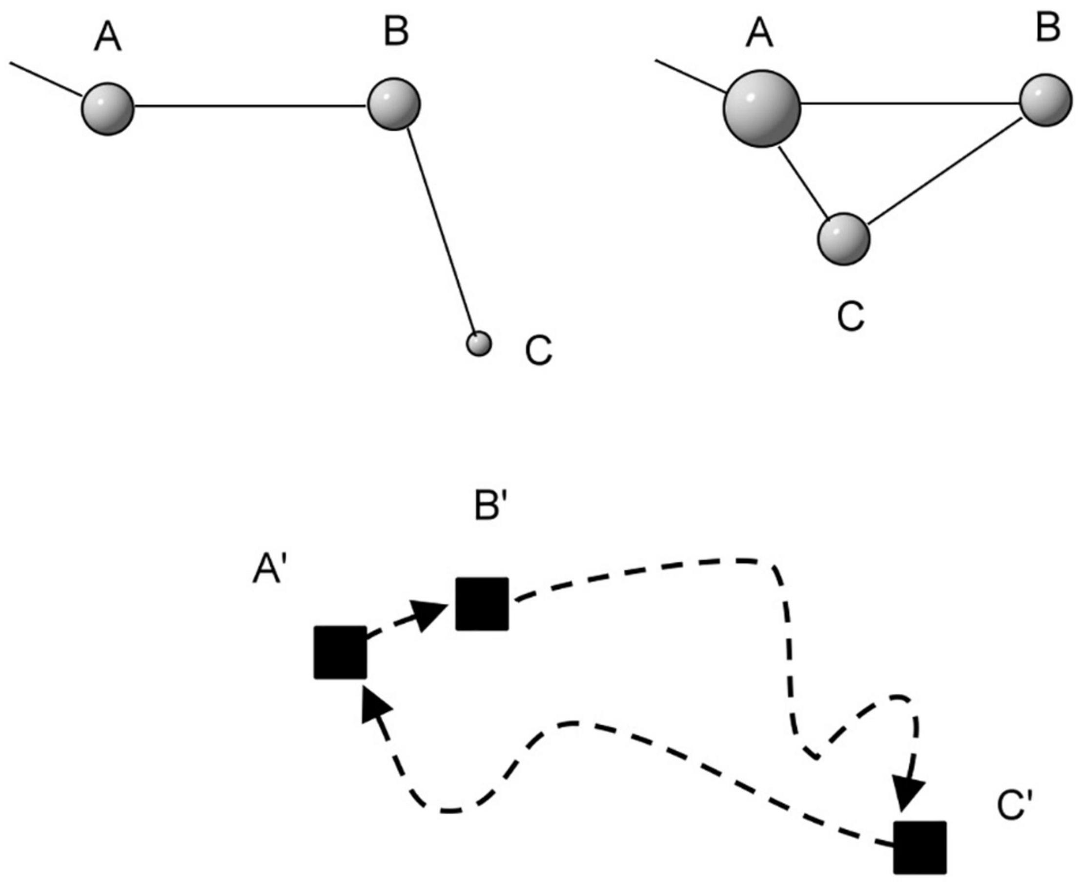
Figure 1. In a virtual network, if the animal revisits a node from another node the topological distance between the two nodes is shortened in an incremental manner for each such revisit between the two. Such return events represent inter-node attachment growth. Short-cuts where for example the individual moves in the node sequence A-B-C-A contributes to increasing the connectivity strength (called the degree, illustrated as bullet size in the illustration) of the revisited nodes. When the animal returns directly to A from C, node A is advancing upwards in the hierarchy of node connectivity strength, which is shown by the new connecting line segment from C to A. This new connection means that A and C also move closer in network topological terms. In contrast, the physical (Euclidean) distance between nodes A, B and C (the “patches” A’, B’ and C’ in the lower part of the illustration) remains the same regardless of node degree and respective topological distances. Along the dotted path only A’, B’ and C’ belong to the network due to previous revisits, while the rest of the path (dotted line) represents potential nodes with still unrealized connectivity to the network of actual nodes.

For the present context of cognitive movement ecology I label the scenarios ‘‘Site Fidelity Network’’ (SFN). Analyses of both the SFN topology and the space use pattern in Euclidean terms are performed under two premises; a statistical-physical level of system abstraction, and application of MRW, which embeds both occasional returns to previous locations and a scale-free distribution of exploratory step lengths.²

The emerging system of site fidelity from an individual entering an area, the animal’s home range, is growing in spatial extent over time due to the mixture of exploratory moves and occasional return events, but much slower in comparison to movement in the absence of site fidelity. From the topological perspective, SFN exemplifies growth of an individual-centric virtual network where new network nodes appear in two variants; (a) nodes that immediately connect to the network and contribute to its growth, and (b) potential nodes. Steps leading to immediate node growth imply that the individual is revisiting a location, starting from a location that so far has not been revisited. The latter then becomes part of the evolving network due to the return event. Thus, only return events from locations outside the present network of revisited nodes contribute to network growth, while returns from an existing node to another node contribute to strengthening the relative degree of the target node (Figure 1). In this case both the start and the target locations were already part of the network. On the other hand, locations that have been visited only once represent a pool of potential nodes. These locations do not immediately link to the present network of actual nodes, but are remembered and may thus connect to the network later on. This aspect of spatio-temporal memory makes it necessary to extend the architecture of classic network topology to the SFN-specific topology, containing both “insiders” and “outsiders.”

From the topological perspective, compliance with a scale-free network distribution of node weight (relative popularity of revisited nodes) regards an emergent property from the movement model’s definition of return events under a premise of network growth; i.e., system openness. A wider the distribution implies a deeper hierarchical depth of node weights. Further, the topological distance between nodes, as exemplified by the length of the connecting lines A to B, B to C and C to A between nodes in Figure 1, is independent of the physical step length distribution per se (distances between successive steps between given time increments; exemplified in Figure 1 by the three distances A’ to B’, B’ to C’ and C’ to A’). Thus, with respect to the scaling properties of node weights, any movement algorithm involving memory-based return events could be applied, given that the properties are studied from the topological side and not from the Euclidean spatio-temporally side. On the other hand, in Euclidean terms, “scale-free” is a property of the movement process in physical space, as defined by the MRW model’s step length algorithm (see below). Similar to the Internet-related example above, a distribution of step lengths obeying P(k) ≈ k^–γ is scale-free over the range of the part of P(k) where γ is stable, and is said to be complex over this range. In step length terms, we study the distribution of binned step lengths. In other words, when log-tranforming the distribution of step lengths one should expect a linear relationship. Thus, two complementary aspects of “scale-free” space use are scrutinized in this report—topological and Euclidean.

How to link an animal’s emerging network topology to its spatio-temporal pattern of site fidelity? Distinguishing between true network nodes from memory-based, intentional return events and exploratory moves that just happen to revisit a site by chance (random path crossing) becomes a challenging and probably unsolvable empirical task, in particular, when these nodes are shifting positions in space over time (“drifting site fidelity”). Still, the cognitive process behind targeted returns leads—in overall terms—to a qualitatively different kind of space use process than movement where each return happens by chance; i.e., independent on memory map utilization. In this report I propose and explore an alternative way to resolve this empirical challenge to differentiate between intentional and random returns. I show how simulations involving memory and site fidelity where properties are known from the given model conditions may reveal important statistical aspects of this kind of space use dynamics.

Given the issues just outlined, the aspect of self-reinforcing use of a subset of nodes in network terms needs to be studied indirectly from the spatial distribution of fixes in physical space, including how such pattern of site fidelity may evolve and change over time. This is where the Euclidean properties of the space use model become crucial, complementing the topological aspects of site fidelity as introduced above. In particular, I show how the abovementioned challenge to pinpoint actual return events from non-intentional returns to specific locations selection may be circumvented by analyzing space use in a statistically “coarse-grained” manner; i.e., from the perspective of statistical physics. This approach may thereby reveal topological aspects of site fidelity indirectly, by observing the system’s complementary properties of the spatio-temporal movement pattern rather than the network topology directly. However, the applicability of this approach critically depends on the realism of the space use model that is applied.

The Multi-Scaled Random Walk Model

MRW simulates movement to be studied at a coarsened temporal resolution; i.e., at a temporal unit scale which is coarse enough to ensure that successive steps are randomly distributed in directional terms. This satisfies the premise of a statistical-physical observations of the process in a more simplified mathematical context, relative to studying the process at finer (“hybrid”) temporal resolutions where deterministic, “tactical” behavior and directional step persistence becomes more influential on the movement path (e.g., correlated random walk). The return steps are memory-dependent and describe site fidelity. What regards the statistical-physical aspect, analysis of individual space use is typically based on fixes that are collected at large time intervals relative to the temporally fine-grained deterministic behavioral response time for successive movement-influencing events within the animal’s current field of perception. For example, GPS fixes from vertebrate space use may be collected at intervals of 1–2 h or larger, embedding much intermediate, tactical and unobserved movement behavior. Thus, theoretical simulation and the accompanying analysis of the space use process at this coarsened “strategic” temporal scale is statistical-physical by nature and in compliance with common empirical protocols.

Three main arguments support the choice of MRW as the basic statistical-physical model for memory-implemented space use. First, based on analyses of real data, area demarcation (home range, A, using various demarcation methods) has been shown to satisfy the MRW-characteristic power law A≈ N⁰.⁵ for all species we have studied so far, for example including free ranging sheep Ovis aries (Gautestad and Mysterud, 1993, 2012), black bear Ursus americanus (Gautestad et al., 1998) and red deer Cervus elaphus (Gautestad et al., 2013). A similar power law compliance was also found in a meta-analysis embedding many vertebrate species (Gautestad and Mysterud, 1995) and recently also in a pilot study on roe deer Capreolus capreolus, based on data from Ranc et al. (2020).³

Second, by superimposing a virtual grid on the spatial scatter of relocations and counting the number of grid cells containing one or more fixes (incidence, I) as a function of grid resolution (a common approach to observe complex space use from a statistical-physical perspective), we have also consistently found a power law relationship, from which we could estimate the fix scatter’s fractal dimension, D. Typically, we find D ≈ 1, which indicates that fixes are statistically distributed in a scale-free (self-similar) manner. In other words, fixes tend to show aggregations over a range of spatial resolutions. This range of the fractal dimension describes a strong aggregative tendency due to D < < 1.5 (Gautestad and Mysterud, 2012; Gautestad et al., 2013), which again is an indicator of positive feedback with respect to local habitat utilization and thus behavioral complexity in statistical-physical terms. Consequently, in our analyses the overall empirical results are MRW-compliant also from this perspective. In other words, some parts of the home range under study were visited more often than others, and this pattern repeated itself statistically in what is called a self-similar (“fractal”) manner toward finer resolutions, apparently not mirroring a simple linear proportionality with local habitat attributes like food resources at respective resolutions. In short, since the estimate of D covers a set of fixes that is collected from a range of local and temporal conditions, the within-range habitat heterogeneity effect on D is effectively “averaged away” from the spatio-temporal pooling of fixes when estimating D.

Third, when the successive fix distances from red deer movement were analyzed (“step lengths,” L, at 2 h time resolution), we found that a power law fitted the distribution F(L) better than the negative exponential, where the latter would be expected from a scale-specific and classic random walk-like kind of movement rather than scale-free space use (Gautestad and Mysterud, 2013; Gautestad et al., 2013). Thus, both small and very large displacements were more common than expected from classical movement models, and again in compliance with MRW properties. A pseudo-scale-free variant where the animal is switching between different scale-specific movement modes—making the total distribution look power law-like (composite random walk) was discarded as explanation of these data (Gautestad and Mysterud, 2013). Recently these aspects of complex space use, expansion of space use, A(N), fractal self-similarity of site fidelity, and the frequency of inter-step movement lengths F(L), have been verified empirically and explored theoretically also by other researchers (Boyer et al., 2012; Boyer and Romo-Cruz, 2014; Boyer and Solis-Salas, 2014; Evans et al., 2019).

In short, the scale-free property of movement steps follows from the model premise that the animal under MRW conditions is assumed to relate to its environment at many spatio-temporal scales in parallel over a given scale range (Gautestad, 2021). In contrast, the classical use-availability analysis of habitat selection is based on a premise of independent revisits to respective sections of a home range; i.e., a memory-less and area-constrained process in cognitive movement terms (Boyce et al., 2002), and the behavior is consequently assumed to comply with some variant of standard (Brownian motion-like or Lévy walk-like) random walk properties in statistical-physical terms. This paradigm premise is neither compatible with an evolving network of nodes, nor compatible with the MRW model, which is formulated to be compliant with evolving memory map utilization and a scale-free kind of space use at the statistical-physical level.⁴ Thus, the present analyses not only explore the feasibility of the MRW model to reveal complex patterns of site fidelity, but also contribute to highlight the fundamentally different system premises on which MRW rests, relative to standard space use models.

To summarize, a theoretical framework to study cognitive movement ecology under condition of spatial memory and scale-free habitat utilization is beginning to emerge, and the MRW seems to be a feasible model platform to study site fidelity in the context of habitat selection (Gautestad, 2015, 2021). The MRW model provides opportunities to indirectly reveal the dynamics of site fidelity under various conditions: both from the network-topological and the Euclidean (spatially explicit) perspective.

In particular, from behavioral-ecological arguments one should expect the return probability to specific sites to decline as a function of increased uncertainty of site profitability or increased risk in connection with return to historic locations; e.g., due to increased environmental variability and unpredictability, or due to a predator’s local search map being influenced by learning the prey’s habits. On the other hand, site familiarity provides crucial benefits with respect to utilizing a memory map (Piper, 2011). These aspects will be scrutinized by the present simulations by varying the temporal stability of existing memory-based targets for an individual’s return events. A sub-set of previously published telemetry data on 15 black bear females (Gautestad et al., 1998) is also explored with respect to the present method to reveal degree of (in) stability of site fidelity.

Materials and Methods

Network Topology Under Site Fidelity Network Terms

Within the area traversed by an animal, some locations may over time be re-utilized in a self-reinforcing manner at the expense of proportional use of other patches of a priori similar qualities—owing to the process of occasional but directed returns to known localities (Gautestad and Mysterud, 2010b). This very general property of vertebrate movement may be simplified into parsimonious model algorithms to simulate memory-enhanced space use.

In general terms; i.e., whether MRW or another kind of statistical-physical algorithm is applied to simulate memory-involving animal space use, the model defines a return step protocol. For example, on average every μth time increment (μ > > 1) in the simulated series the given step is followed by a directed return to a randomly and uniformly distributed chosen previous location in the series (called “neutral connectivity”). Alternatively, the protocol could define “preferential connectivity,” where visited locations gain increased probability for additional revisits. Anyway, the probability for a revisit to a given site under the chosen connectivity scheme on average declines geometrically over time, due to an incrementally larger pool of potential return targets as the total path expands. A large μ indicates that returns happen at a low frequency relative to exploratory steps, but from a topological perspective μ does not influence the distributional form of the actual node weights, only the relative magnitude of potential nodes in comparison to the smaller but evolving set of actual nodes (network growth). The reason is that the size of the network grows as a function of actual nodes. Thus, the speed of this growth depends on the frequency of returns, 1/μ; i.e., smaller μ implies relatively stronger growth, but the distribution of node weights (its power exponent) does not.

The network topology of actual, inter-connected nodes—based on the set of return target locations—were studied by analyzing the so-called degree distribution and the accompanying weight of nodes (popularity): frequency of nodes as a function of connectedness (number of returns to a given location), which also increases some nodes’ weight on expense of less visited nodes. Gephi version 0.7 alpha2 and version 0.9.2 (Bastian et al., 2009) were used in these analyses.

In practice, series of simulated return targets and the respective locations from which the individual initiated a given return event were successively separated from the developing path series into a two-column spreadsheet, which was then imported to Gephi for analysis. In order to reveal the degree of power law compliance, the degree distribution of node weight was subject to geometrical binning. Further, the spatial locations of the most “popular” nodes were superimposed on a dispersion of a set of fixes, in order to illustrate—in phenomenological terms—the juxtaposition of these locations with relatively high return frequency relative to the over-all spatial pattern of fixes.

Only the first 10⁴ return targets in each series of 10⁵ or 10⁶ MRW steps using returns at every μ = 10 time steps on average were analyzed for scaling properties, due to their strongest network maturity; in the initial part of the step series had the longest history of return events and consequently providing the highest analytical potential to distinguish a scale-free or approximately scale-free; i.e., an approximately log-log linear degree distribution, from scale-specific network topology (semi-log linear). The latter parts of the series consisted mainly of potential nodes (not yet part of the set of actual nodes due to lack of becoming return targets). By comparing the network graph of the first 10⁴ return targets from a 10⁵-step series with the graph from the first 10⁴ return targets from a 10 times larger series one gets a qualitative impression of how the “hierarchical depth” of the graph is progressing as the SFN evolves over time.

Balancing Exploration and Site Fidelity in Euclidean Space

Above I have already given the three main arguments for choosing MRW as the basic model when flipping from network topology to the Euclidean properties of memory-influenced space use. Under the premise of the MRW framework, space use emerges from a combination of exploratory moves and occasional returns within a defined time resolution and spatial extent. What regards simulation of exploratory steps of space use, MRW series of length 2*10⁷ steps, representing successive path locations at the defined unit time interval t, were simulated in a homogeneous environment as a set of successively independent step vectors of length:

$L{}_{MRW}=\mathrm{\alpha }(RND){}^{-}{}^1{}^{/(}{}^{\mathrm{\beta }}{}^{-}{}^{1)}|L{}_{MRW}<L_{\mathit{max}}(1)$

with α = 1 and β = 2. RND is a random number between 0 and 1. Hence, median step length is 0.5^–1 = 2 length units. The maximum step length, L_max, is by default set very large, meaning that this cut-off of step length does not influence the present results. Eq. 1 (without the added property of memory inclusion; see below) is a common formulation of so-called Lévy flight, representing a true Lévy walk that is simulated at a coarsened (statistical-physical) temporal scale, defined by a. A constant α at the unit temporal simulation scale implies a given average step length for the simulations; i.e., movement speed is for simplicity assumed constant on average over space and time during the given time resolution and extent.

From a network perspective, steps from Eq. 1 represent potential nodes and extending this basic algorithm with return steps implements the memory process. This MRW models give birth to a new actual node (targeting a previously never revisited location of the historic path) or contributes to increasing the popularity of an already existing node. Since the first part of the present analyses is targeting the properties of the network topology of popular nodes that emerge for memory-influenced space use, other aspects of habitat interactions (for example, relations to specific habitat elements in a heterogeneous environment, including difference in local movement speed as reflected by differences in the parameter a or difference in the return frequency 1/μ during respective time periods) are for simplicity not specified. This simplification is chosen for the sake of remaining focused on the duality between complexity of node connectivity in topological terms and site fidelity in explicit spatial terms. Running the simulations with millions of steps at statistical-physical resolution is an unrealistically large sample size to represent real individuals. However, this magnitude is chosen to allow for a proper study of theoretical aspects of the system’s network topology and the complementary spatio-temporal properties of MRW.

Under the implicit premise of a statistical-physical system simulation even at unit time scale t = 1, successive inter-step directions of the exploratory steps (Eq. 1) are drawn uniformly from 0 to 2π radians. Before considering the complication from return steps, large series of steps L_MRW represents scale-free distribution of moves (“exploratory steps”), sampled at constant intervals of length t, thus complies with sampling a Lévy walk (Shlesinger et al., 1993; Reynolds and Rhodes, 2009); thus, de facto becoming a series of steps called a Lévy flight.

The log-formatted bin width of the distribution of step lengths from Eq. 1 is set somewhat larger than the median step length in the sample at time resolution t, to study the functional form of the long-tail part of the step distribution at the chosen temporal sampling scale. For example, if median step length is found to be L_med, unit bin width is by default set to be 50% larger.

However, MRW deviates from Lévy walk/flight by adding the effect from spatial memory and site fidelity. This property makes the process potentially scale-free also in the time domain, and not only in the spatial domain. On average every μth time increment in the simulated series the step was followed by a directed return to a randomly and uniformly distributed chosen previous location in the series (neutral connectivity; i.e., the default condition of MRW), or by preferential connectivity, where visited locations gain increased probability for additional revisits. The magnitude of μt (where μ is an integer larger than one) defines the general strength of this “homing” tendency; larger μ implies weaker site fidelity due to longer return intervals on average. Ecologically, a larger μ may for example imply space use under less favorable conditions than where μ is small. In the present simulations with respect to network analysis I used 10 < = μ < = 100 under the condition of neutral connectivity (all historic locations relative to a given instant has equal probability for a revisit). For Medium preferential connectivity I used an added condition that returns either takes place with 50% probability to a randomly chosen target among existing network nodes; i.e., a location that has already been visited before, and 50% probability for returning to a randomly picked target regardless of status. This implies a “preference” to return to already revisited locations relative to neutral connectivity. For Strong preferential connectivity I used 90% probability to return to an existing, actual node and 10% to a randomly picked location (using 100% return to actual nodes would terminate network growth). Thus, the choice of 50 and 90% strength of preference represents two levels of skewedness on the continuum from 0% (neutral connectivity) toward—but not including—100%). With respect to spatio-temporally varying site fidelity (next section), I used μ = 100 for all conditions of connectivity strength.

Further Coarse-Graining of the Process: Fix Sampling and Analyses

Each series was sampled as one “observed fix” (t_obs) pr. 1000t; i.e., a coarser time resolution than the average return interval at the scale of steps at unit time resolution, t (t_ret = μt = 100t) in the simulations of varying site fidelity. Hence, intrinsic serial auto-correlation was effectively eliminated at the temporal scale of t_obs > > t_ret.

Sets of fixes from each series were in the present context collected at temporal scale t_obs = 1000t. Thus, analyses of movement in physical space represents a small subset of the original path; in contrast to the introductory study of network topology (above), which were analyzed at unit scale t = 1.

Incidence, I, which represents the number of virtually superimposed grid cells embedding at least one fix, is applied to quantify spatial use in an Eulerian (spatially explicit) manner. While traditional estimates of home range area A(N) where A is given by an area-demarcating method, have many complicating challenges, the I approach allows for a coherent fractal-geometrical analysis of the spatial fix pattern. The sample size dependence of incidence as a function of sample size of fixes, I(N), at a properly chosen resolution of grid cells called the Characteristic Scale of Space Use (CSSU)⁵ (Gautestad, 2021), can under MRW be expressed by the power law (Gautestad and Mysterud, 2005, 2006, 2010a):

$I(N)=cN{}^z(2)$

where c and z are parameters. The intensity of habitat utilization is expressed through the combination of c and z; c regards CSSU, and is—under a given average step length of exploratory steps—a function of the frequency of returns, 1/μt, to previous locations (space use intensity). CSSU is thus expressing the behavioral balance between space use expansion (exploratory steps; Eq. 1) and contraction (site fidelity from returns at frequency 1/μ). The parameter z expresses how intensity of space use is distributed across scales. Stability of z implies a scale-free kind of relationship to the habitat over a range of spatial resolutions of the environment. A value of z ≈ 0.5 [I(N) increasing proportionally with square root of N] implies by a MRW postulate that the animal is “relating” to its environment over a range of scales with the same space use intensity; i.e., a next-step movement to a neighborhood at a k² times coarser scale is 1/k² times less probable (Gautestad and Mysterud, 2005).

Theoretical expectancy is z≈0.5 for the idealized MRW (Gautestad and Mysterud, 2010a), with some variability expected from so-called space-fill and dilution effects from choosing too coarse or fine grid resolutions, respectively (Gautestad and Mysterud, 2012). In other words, the analysis should be performed after having “zoomed” grid resolution to a magnitude close to CSSU. Zooming to estimate c is necessary due to the process’ combined expression of exploratory steps (influenced by a and β in Eq. 1) and return step effects. Too coarse or too fine grid resolution relative to the intrinsic CSSU scale will both lead to observed instability of c and z over the range of N (see a practical example in Supplementary Material).

The sample size of fixes, N, can be drawn incrementally from the total series in two ways; either by adding new fixes in a time-incremental manner (continuous sampling; a sample size that is proportional with sampling time) or by increasing sampling frequency within the total time period for the simulation (including every nth fix within the total time period, by increasing n until n = N). In the present analysis I—crucially—applied both protocols, and additionally calculated the geometric average of I(N) for each magnitude of N from these alternative sampling schemes.

In this manner, by averaging I(N) over continuous and frequency sampling and studying the difference between the non-averaged I(N) series from the two protocols, one may compare the statistical effects from intrinsic auto-correlation in the data (t_obs <= t_ret) with the statistics of the non-averaged I(N) series. The differences will be of key interest to the present topic of quantifying the effect of extrinsically induced autocorrelation even when t_obs > > t_ret, due to an environmentally imposed shifting mosaic of site fidelity.

In addition to the CSSU concept and its relationship with Eq. 2, memory effects under MRW terms impose yet another aspect of space use intensity; the property of self-similar (fractal) dispersion of fixes. In other words, a sample of fixes from the underlying process combination of Eq. 1 in combination of targeted return steps will tend to be spatially distributed as aggregations over a range of resolutions of the superimposed grid (in contrast, Eq. 2 is expressing the N-dependence of incidence at given grid resolution; the balance scale of CSSU). For non-auto-correlated fix samples we have shown theoretically and verified by simulations (Gautestad and Mysterud, 2010a) that,

$z=1-D/2\mathit{\hspace{1em}\hspace{1em}\hspace{1em}\hspace{1em}}|1<D<2,N>N{}_{mi}{}_n(3)$

where D is the fractal dimension of the spatial distribution of fixes. N_min approximates a small-sample artifact of N. D can thus be calculated from D = 2(1-z), as an alternative approach to zooming over a range of grid resolutions (see section “Introduction”).

Combining Eq. 2 and Eq. 3 gives,

$I(N)=cN{}^{1-}{}^{D/}{}^2|N>N{}_{min},I\equiv incidence(4)$

In particular, D≈2 implies I(N) is constant beyond N_min. This satisfies the paradigmic “home range size” concept, where the size is assumed to expand asymptotically toward the range’s size as N is passing N_min from below. On the other hand, D≈1 implies I(N) is increasing proportionally with N^1/2 far beyond N_min. In practice, N_min is very small under D≈1 relative to D≈2 dispersions, since the latter is more “dense” in statistical-fractal terms and thus require a larger set of fixes to minimize the small-sample artifact of I(N).

In the present context, c is the most important ecological aspect of the model. Representing CSSU, it reflects the characteristic scale of space use intensity on average within the respective spatial and temporal scale extents:

$c=I(N)/N{}^{1-}{}^{D/}{}^2=I(N)/N{}^z(5)$

Under condition of z≈0.5, a larger c implies a more coarse-grained CSSU on average in the spatio-temporal range that is embedded by the data.

Non-stationary Site Fidelity

In the present simulations the parameter values for a and β in Eq. 1 (exploratory steps) and the return frequency to historic locations (relative strength of site fidelity, 1/μ) are kept constant. However, as indicated above, extrinsically imposed serial auto-correlation of fixes may influence the observed statistical properties of space use. Thus, in this report I study to what extent the resilience of key statistics under the given model parameters under default (stationary) conditions are influenced by a shifting mosaic of site fidelity.

To simulate a varying environment with respect to influencing stability of site fidelity and—in particular—whether this environmental heterogeneity is influencing c and z (or conversely, how resilient these parameters are under increased environmental complexity), three conditions are explored by varying strength of so-called “punctuated site affinity.” At regular intervals (the punctuations) the model individual is narrowing its time horizon for memory-influenced movement by disregarding utilization of the older parts of its historic path during return events. At these intervals the movement path is thus simplistically split into “sections.” Older parts of potential nodes are not any longer included in the process of return decisions. However, it continues to return to a given percentage of the latest part of the foregoing section in addition to all the new locations in the current section. By varying the length of the sections and the length of the retained part of the foregoing section, a variable strength of spatially shifting site fidelity may be simulated (Gautestad and Mysterud, 2006).

Under the first condition, A, the animal is keeping the last 10% of the path locations in foregoing section of the path, each of length 1/10 of the total series length of magnitude 10⁷ steps, as potential return targets on equal footing with the successively emerging locations in the current section. The simulations are run under condition of neutral connectivity of return events.

Under the second condition, B, 50 rather than 10 time sections for partially punctuated site affinity is invoked, and 2% rather than 10% of the previous section’s path of locations is retained (section length 2*10⁵ steps, and last 4*10³ steps of foregoing section retained). This condition implicitly reflects a situation where site fidelity is drifting more smoothly but also more strongly in overall terms than in the foregoing scenario, due to a smaller subset of previous locations to select among as return targets and a more frequent resetting of potential return targets. The simulations are run under condition of neutral connectivity of return events.

Under the third condition, C, drifting site fidelity is similar to A, but with no memory of previous sections. Number of sections is increased from 10 to 20, but no historic parts of the path of 1/20 of total length is retained during this fully expressed “punctuated shift” of site fidelity. The first location in each of the 20 successive sections is chosen randomly within the total arena. This scenario reflects the most dramatic shift of site fidelity. Again, the simulations are run under condition of neutral connectivity of return events.

From each series of locations in the three variants of shifting site fidelity, each variant replicated 10 times, fixes are sampled at frequency 1:1,000 of respective series. Within each sequence of stationary site affinity; i.e., in the respective sections between the successive punctuation events during which the conditions for site fidelity were temporally stable, this situation implies serially non-autocorrelated steps (Swihart and Slade, 1985). However, this condition is expected to change to serial autocorrelation as the data set embeds several re-settings of site fidelity (fixes covering several sections) and thus a spatially drifting space use. Thus, auto-correlation may emerge under the respective conditions of temporally non-stationary space use, because of two random locations within a section may tend to be closer in space than two locations from different sections in the total set of fixes. In short, auto-correlation is expected to occur even under the condition where t_ret = μt = 100t is set to be smaller than the fix sampling interval t_obs = 1000t, because of the temporally shifting pattern of site fidelity (extrinsic forcing).

A resolution of the virtual grid that is superimposed for the analysis of I(N) is fixed for all simulations (k = 1/40, linearly, of total arena scale of k = 100,000). This resolution approximates the CSSU scale under the given model conditions prior to adding the complexity from drifting site fidelity. In other words, log(c) approximates zero after normalization to linear grid resolution of k = 100,000/40 = 2,500 units.

All conditions A, B and C above were simulated under neutral connectivity. In order to explore the effect of preferential connectivity in isolation from drifting site fidelity, I(N) for strong preferential connectivity is also analyzed as condition D; i.e., under standard MRW terms for return events (site fidelity not influenced over time by external forcing).

Pilot Testing on Telemetry Series

With respect to illustrating the new method on empirical data, a sub-set of previously published telemetry material on female black bear is presented with respect to I(N), including the stability and distribution of c and z from Eq. 2. According to the MRW framework, z should be independent of both c and N after respective series are zoomed toward best-fit scale for CSSU estimation. The data is reflecting standard radio telemetry procedures and equipment from the 1970s, reflecting both relatively large triangulation errors and subsequent rounding of fix coordinates to nearest 100 meters. Fixes were collected at intervals of one or more days. For details of the telemetry material, see Gautestad et al. (1998).

Results

Network Topology

The MRW simulations with respect to network topology of nodes and neutral connectivity illustrate compliance with a gradually emerging hierarchical depth of these nodes. Some of the initially appearing nodes gain further revisits, in a positive feedback-resembling growth process (Figure 2A). Over time, an understory of additional hierarchical layers of nodes with less revisit frequency appears, while most nodes are visited only once (Figure 2B). The first 10³ links were generated from 10⁴ to10⁵ return events to previous locations along the animal’s path (total series length 10⁵ and 10⁶ respectively, due to t_ret = 10t). Under neutral connectivity, in the early stage of space use (Figure 2A) most nodes have only one link, and the number of hierarchical levels is limited to four. By increasing the series length 10-fold (Figure 2B) the structure of links (the degree) to the initial 10³ nodes has become more complex with six levels, and thus reflecting a more mature network with respect to its hierarchical property. The temporal drifting toward a scale-free topology is indicated by the rarity of nodes with a large degree relative to the large population of low-degree nodes. Whether this is actually scale-free or not depends of compliance with a power law in the distribution of connectivity strength (see below). However, this example illustrates that even neutral connectivity leads to re-use of sites in a self-reinforcing manner due to the site’s added statistical weight with respect to the probability of becoming target for new visits.

FIGURE 2

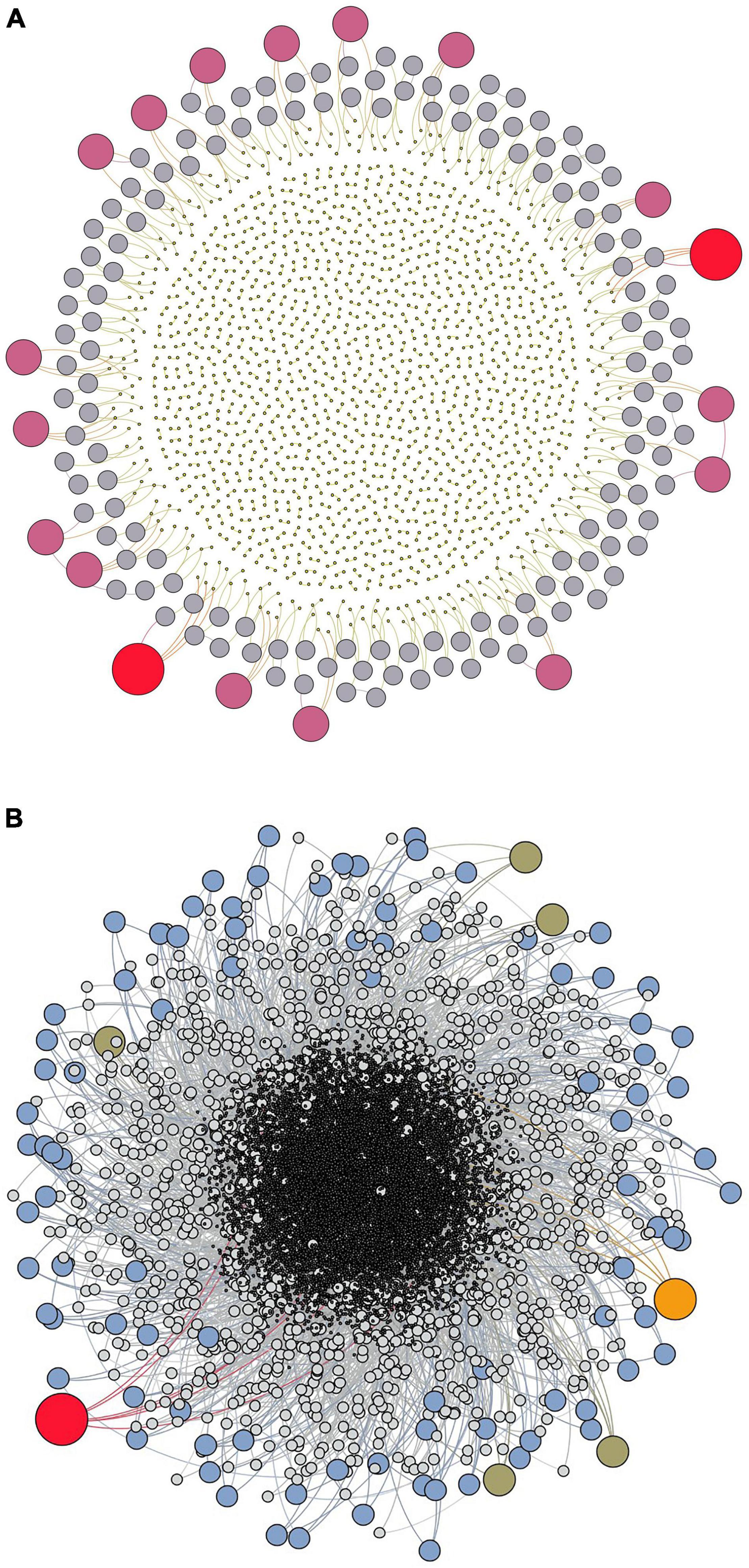
Figure 2. Network graphs (produced in Gephi 0.8.2 and 0.9.2) (Bastian et al., 2009) illustrate how a site fidelity network (SFN) even under neutral connectivity becomes increasingly complex by increasing number of hierarchical levels of connected nodes (re-used locations) over time. Each series consists of 10⁴ steps with a new potential or realized node creation every 10 step on average (t_ret = 10). Node degree is expressed by the size of the bullets, while colors only serve to distinguish the respective magnitudes of degree. (A) The center part of the network visualization represents Level 1, containing nodes with only one connecting link (smallest network fragments). (B) The link structure of the initial 10⁴ return events of a series of 10⁵ steps becomes more complex with more levels when studied as the initial sub-section of a 10 times larger series than in (A). In other words, the network is more “mature” owing to the longer time span of development of the initial part of the network.

Before leaving the topological aspects, Figure 3A exemplifies a MRW simulation under stationary site fidelity and neutral connectivity, and how the network of nodes is dispersed in space. The actual spatial locations of the five dominating nodes—super-nodes—are marked by colored squares. Hierarchical node dominance is not clearly correlated with local density of fixes (local “core areas” of more intense use, called the utilization distribution in home range theory). This apparent independence between node degree (connectivity strength) and strength of the utilization distribution in Euclidean space is illustrated by the locations of the two peripheral nodes in relatively low-density regions of the scatter of fixes, which reflects not only the actual nodes but also the dispersion of potential nodes. This result may seem counter-intuitive from standard home range premises, but is in fact expected from the simulation’s condition of MRW’s independency between a start location for a return event and the target’s temporal sequence position in the series. While this example shows super-node distribution under neutral connectivity, a similar pattern in qualitative terms appeared under preferential connectivity (not shown).

FIGURE 3

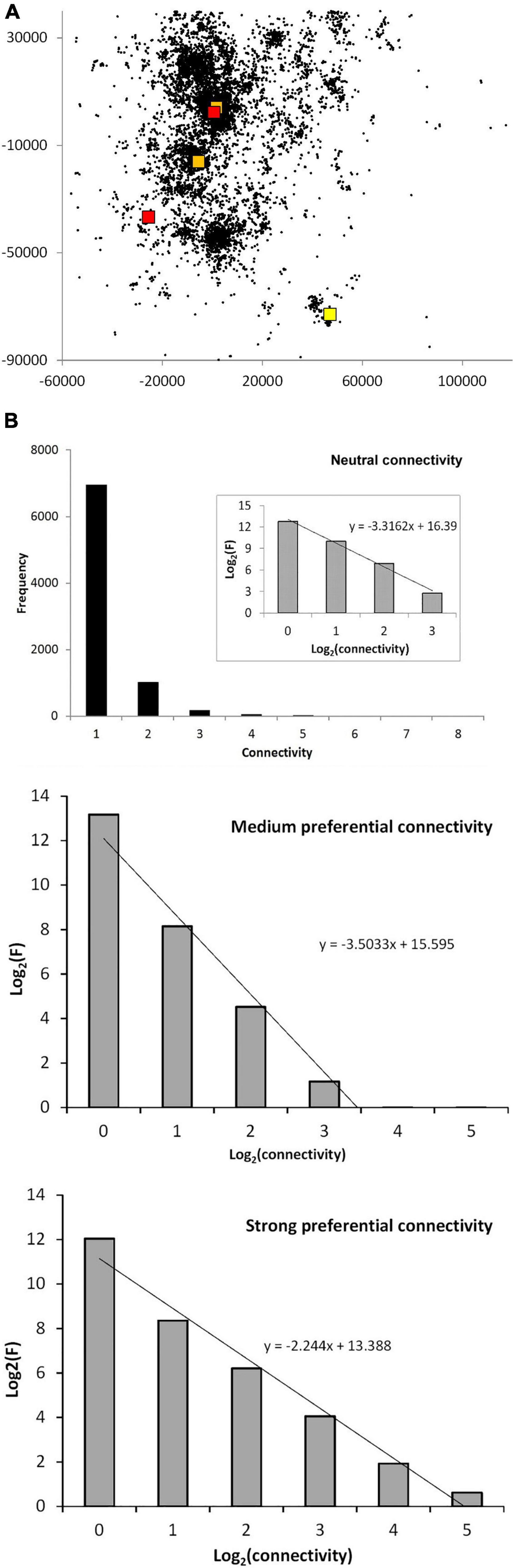
Figure 3. (A) The scatter shows the spatial dispersion of a set of simulated MRW locations under neutral connectivity, including both actual nodes (re- visited locations) and other sampled locations of the actual path (representing potential nodes). The path is sampled at frequency 1:1,000 relative to unit time increments. The return interval was set to t_ret = 10. The colored icons locate “super-nodes,” the nodes with the highest node weight; i.e., with largest connectivity strength in the virtual network. Yellow: 8 return events to this location; orange, 7 events (2 locations); red, 6 events. In the latter category only 2 of the 5 locations are shown, since the other 3 were nearly overlapping with another super-node. (B) The degree distribution of node weights (connectivity) for the data in (A) (upper panel), with inset showing log-log transformation. In this inset the super-nodes are included in the right-hand column and part of the second-right-hand column. Ten independent series were produced, and the respective replicates were averaged. The middle and lower panes show the log-log transformed degree distribution for medium and strong preferential connectivity, respectively.

Figure 3B shows the distribution of node degree for the virtual network of the data in Figure 3A (upper pane). The super-nodes represent the right-hand part of the distribution. However, they are few in number. Thus, they become visible only in the log-log distribution (inset), which resembles a power law with exponent β = -3.3. Based on additional simulations, the middle and lower pane give the log-log degree distribution for medium and strong preferential connectivity, respectively (average result from 10 replicate series pr. condition). The latter shows an increased hierarchical depth; i.e., a wider distributional range of node weight, and consequently a reduced slope with exponent β = -2.2.

Spatio-Temporal Space Use Under Drifting Site Fidelity

Under partially punctuated site affinity and neutral connectivity (10 sequences and 10% overlap of targets for returns; condition A) a tendency for drifting home range is apparent from the somewhat lower magnitude of spatial overlap between 100 fixes from early, middle and late part of the series (Figure 4A). However, the spatial drift of space use is weak. Within each of the 10 sequences the animal’s site fidelity is evolving without extrinsically invoked interruption of side fidelity. When the 10 time sequences are analyzed separately in a regression and averaged (Figure 4B), the two sampling conditions under intra-sequence periods give similar-sized average incidence over the range of log[I(N)], with power exponent close to the expected z = 0.5 (z = 0.474, SE = 0.008). The total set of fixes shows a similar average log[I(N)] (z = 0.499, SE = 0.009). These results verifies absence of visible autocorrelation at the intra-sequence temporal scale, but—due to the shown divergence of time-continuous and frequency-based fix sampling for the total set—some magnitude of auto-correlation in the total series embedding a shifting pattern of site fidelity. The similar intercept with the y-axis, log(c) implies stability of the characteristic scale of space use (sequences: z = 0.344, SE = 0.076; total series: z = 0.431, SE = 0.048), CSSU.

FIGURE 4

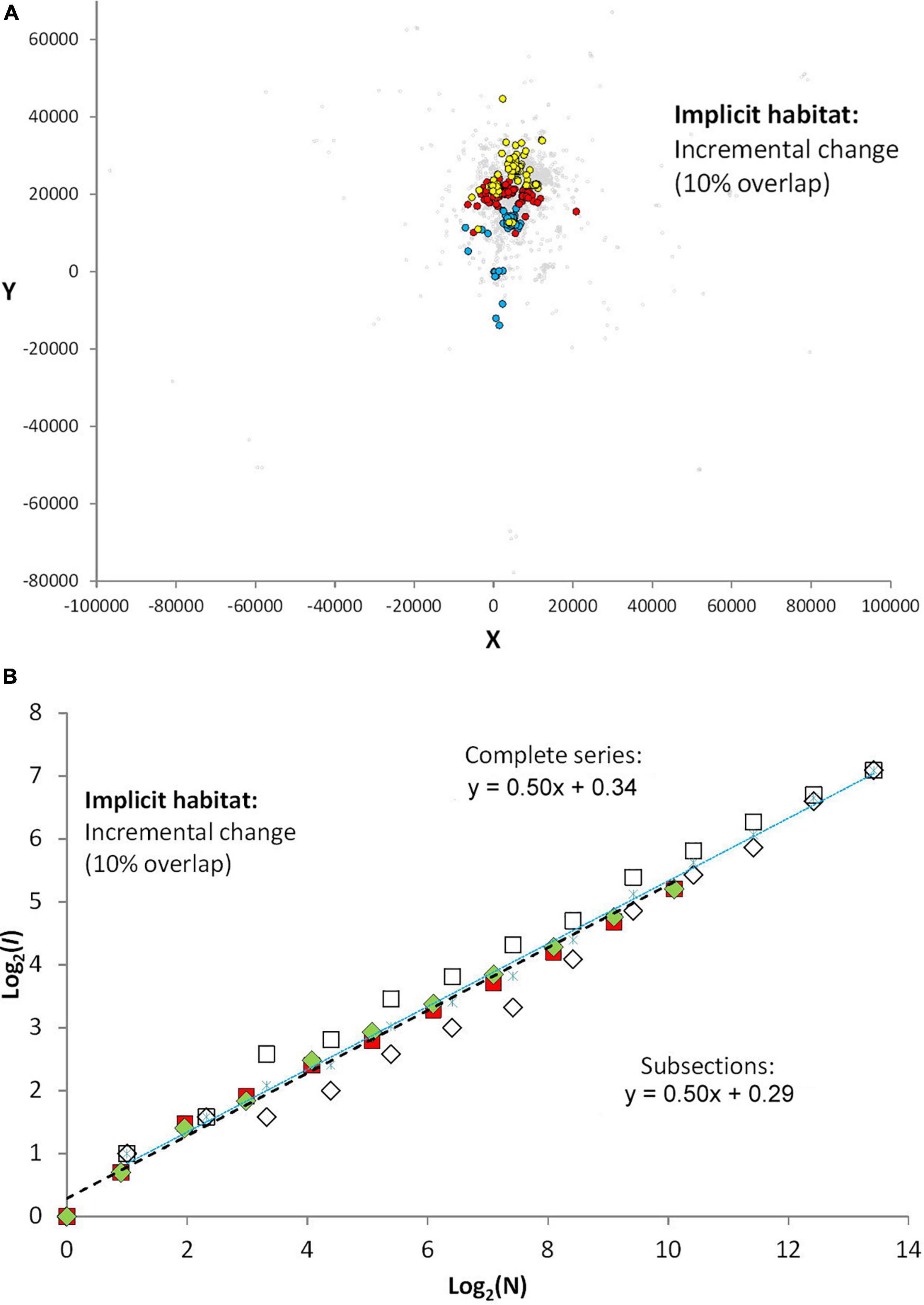
Figure 4. Each scenario in this and the following presentations of simulation results is replicated ten times, and respective plots of I(N) both for time-continuous and frequency-distributed sampling of N are presented. Using the average log[I(N)] over the range of log(N) for the two sampling schemes time-continuous and frequency-based sampling is used to quantify the difference between serially non-autocorrelated and autocorrelated series. The influence on c and z as autocorrelation from extrinsic origin is increased (influencing instability of site fidelity) can also be revealed in each of the three scenarios, by studying log[I(N)] in the respective sections of stable site fidelity between punctuation events where intrinsic autocorrelation is absent due to t_obs > > t_ret. (A) Under partially punctuated site affinity (condition A; 10 sequences, see main text) a tendency for drifting home range is apparent from the somewhat lower degree of spatial overlap between samples of 100 fixes from early, middle and late part of the total series, presented by, respectively, colored dots. (B) The spatial drift under condition (A) is weak, which is reflected in the relatively narrow difference between sampling N fixes by a frequency-based sampling (open squares) or a continuous time scheme (open diamonds). The average log[I(N) is shown as blue stars. When the ten time sequences are analyzed separately (green and red-colored icons), the two sampling conditions give similar-sized incidence over the range of N as the average log[I(N)] from the total set of fixes (the average of the section series is the mid-point between the respective sets of colored squares and rectangles, but is not shown for the section series). The y-intercept, Log(c), under the two sets of analysis is of similar magnitude, both within sections and for the overall series containing all sections.

Second, a more continuous shift of site fidelity (condition B) is shown in Figure 5: returns are limited to a trailing time window that contains the last 2% of locations over a shift every 1/50 part of the total series. Under this condition, the divergence of plots between the two sampling schemes is more pronounced (averaged set: z = 0.57, SE = 0.014).

FIGURE 5

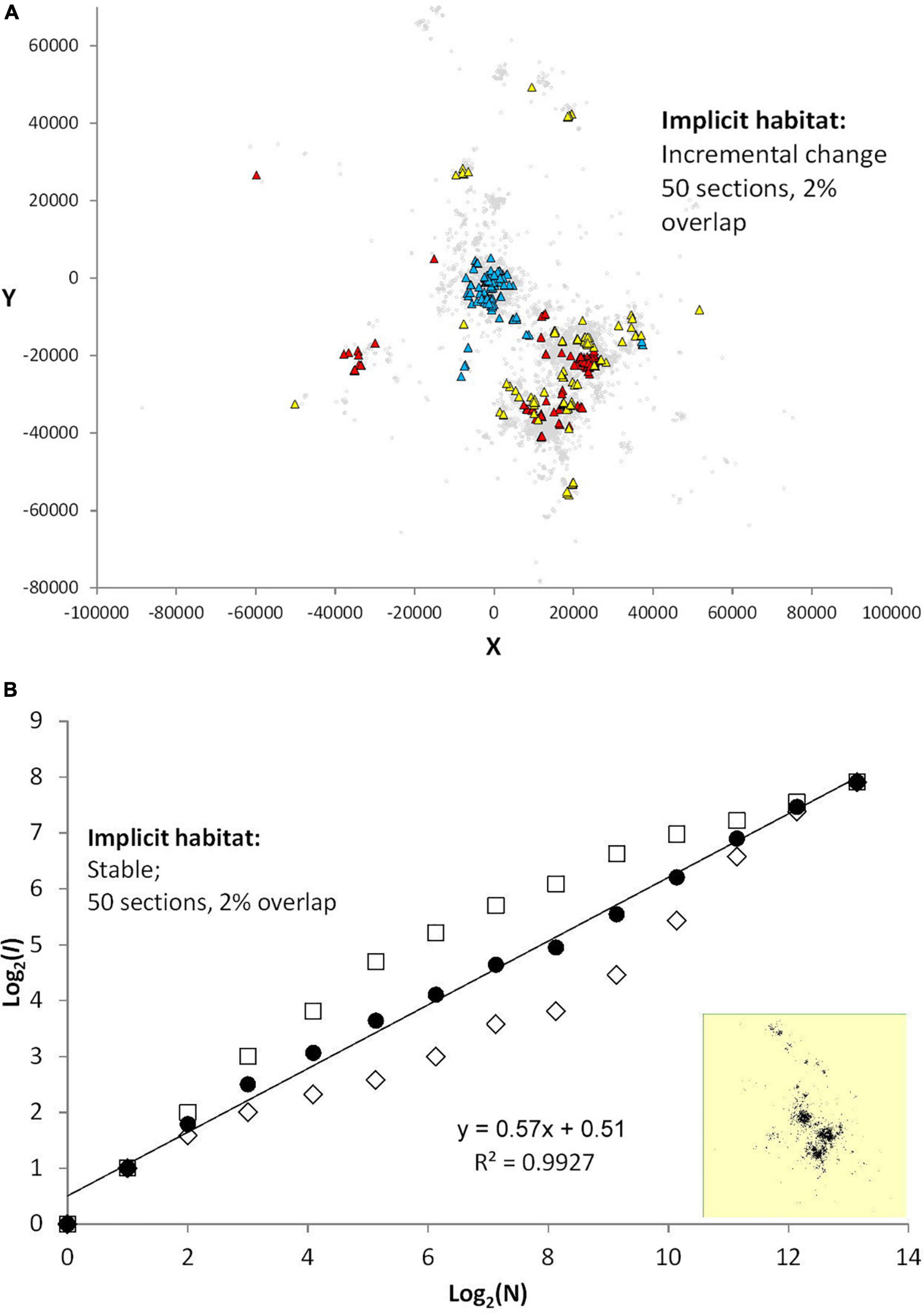
Figure 5. (A) When only 2% of last-section path is retained and the number of sequences for partially punctuated site affinity is increased from 10 to 50 within the same magnitude of total series length (condition B), the drift of site fidelity increases in strength. Consequently, overall space use becomes wider (gray dots relative to the three subsamples shown by colored dots) and the respective N = 100-samples are less overlapping. (B) This effect becomes apparent in the analysis of incidence, I(N), which owing to the stronger spatial auto-correlation shows a widened difference between log(y-intercept) for a given log(N) the two fix sampling methods. However, when log(y-intercept) from the two sampling methods continuous and frequency-based are averaged (filled circles) the slope is—as in (Figure 4—approximately) log-linear and thus power law compliant. As in the foregoing results, log(c) from such averaging seems quite resilient, and thus CSSU seems to be little influenced even by this strongly shifting pattern of site fidelity.

Third, the most dramatic shift both with respect to space use and in the pattern of I(N) under the two fix sampling schemes (condition C) appears where site fidelity is set to re-generate from scratch at every instance of re-setting of site fidelity (Figure 6).

FIGURE 6

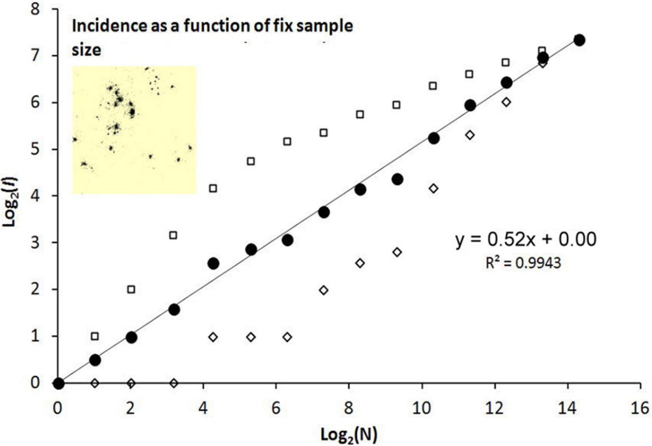
Figure 6. Condition C: site fidelity is set to re-generate from scratch at every instance of re-setting of site fidelity. The inset shows the dispersion of fixes.

In Figure 7, where strong preferential connectivity (Condition D) is simulated under stable (rather than drifting) site fidelity, shows that the scaling slope z≈0.5 seems to be uninfluenced by the magnitude of preferential relative to neutral connectivity (z = 0.535, SE = 0.029). This result is thus similar to the condition of stable site fidelity under neutral connectivity, as was shown within the separate sections presented by green and red icons in Figure 4B. However, CSSU – estimated as c⁰.⁵ = 1000k for medium preferential connectivity and c⁰.⁵ = 667k for strong preferential connectivity—were both smaller than c⁰.⁵ = 2500k under neutral connectivity [not explicitly shown, since in all I(N) presentations, c is calibrated to unit scale; i.e., log(c)≈0].

FIGURE 7

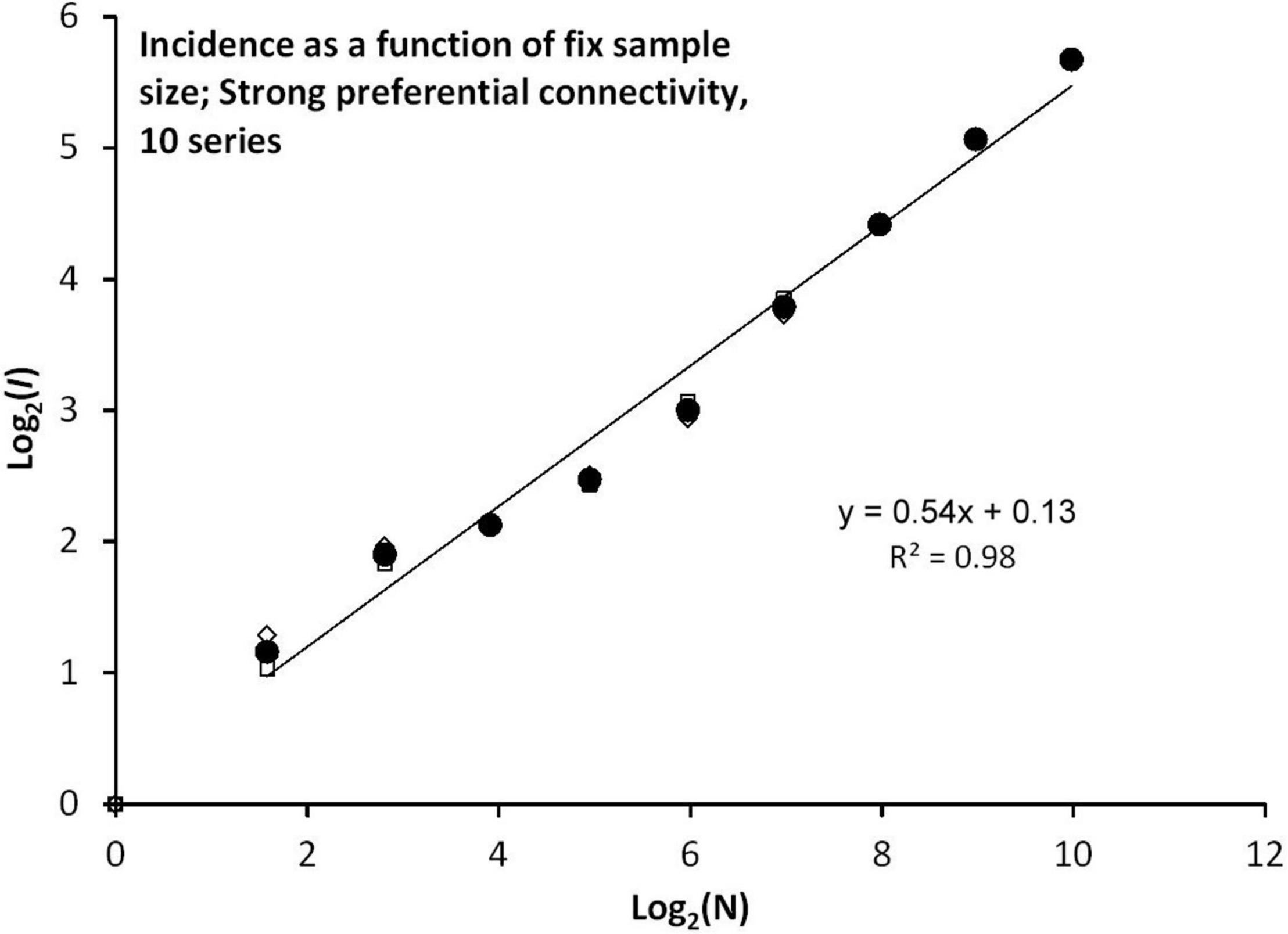
Figure 7. Condition D: I(N) under strong preferential connectivity and no drift of site fidelity (average of 10 series).

Applying the Method on Black Bear Telemetry Data

Figure 8 illustrates by empirical data some of the basic principles that are presented by the simulations. Figure 8 shows the average I(N) for a set of 15 female black bears, showing close compliance with a power exponent z≈0.5 when averaging over time-continuous and frequency sampling of N, and thus in line with the default MRW expectation (z = 0.50, 95% confidence interval 0.46–0.55; SE = 0.02). Divergence between the two sampling schemes indicates some level of serial autocorrelation; i.e., indicating some magnitude of drifting site fidelity. For all plots where log₂(N) > 2; i.e., N > 4, frequency sampling produced larger I(N) than time-continuous sampling. Further, Figure 9 shows that the distribution of CSSU estimates for the 15 series is wide. However, analyses to reveal ecological correlations (like strength of habitat selection) to study the pattern behind respective series were not performed. Crucially, in Figure 9, middle and lower pane, z shows independence of both c (giving the CSSU estimate) and N, as predicted by the model’s basic premises.

FIGURE 8

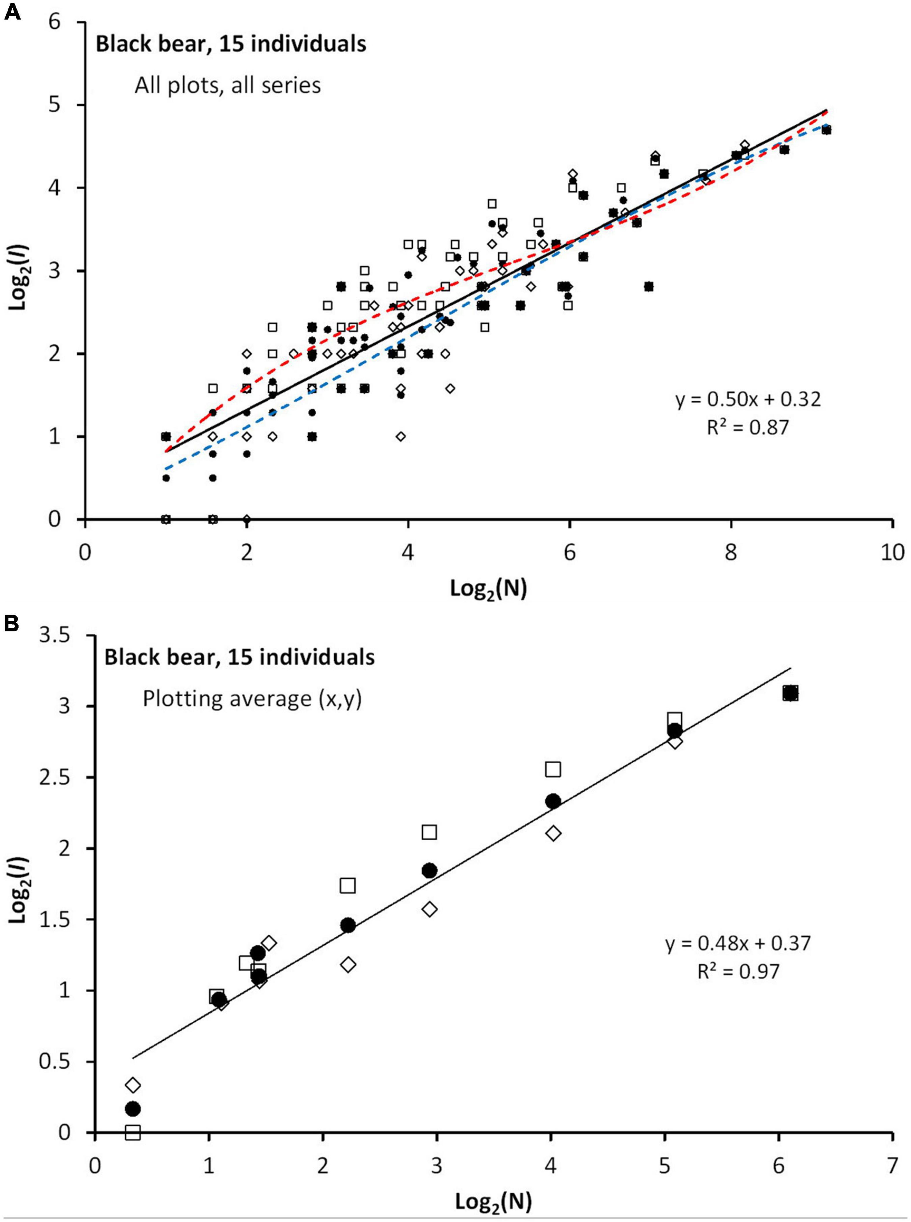
Figure 8. (A) Results of re-analysis fixes from a sample of 15 telemetry series of black bear, where N-dependency for respective series is analyzed by I(N) rather than R/S (see main text). Plots of log₂[I(N)] for time-continuous (diamonds), frequency-distributed sampling (squares) and the log-average of the two schemes (black circles) shows compliance with power exponent z≈0.5 for the latter (continuous line). All sets from all schemes are superimposed, which implies a mixture of series with different N_max. The slight non-linearity of time-continuous and frequency-distributed sampling is visualized by curve-fitting by third order polynomials (blue and red dashed lines, respectively). (B) The divergence between the two fix sampling schemes over the mid-range of N is better visualized by averaging over respective series’ N- and I(N)-plots.

FIGURE 9

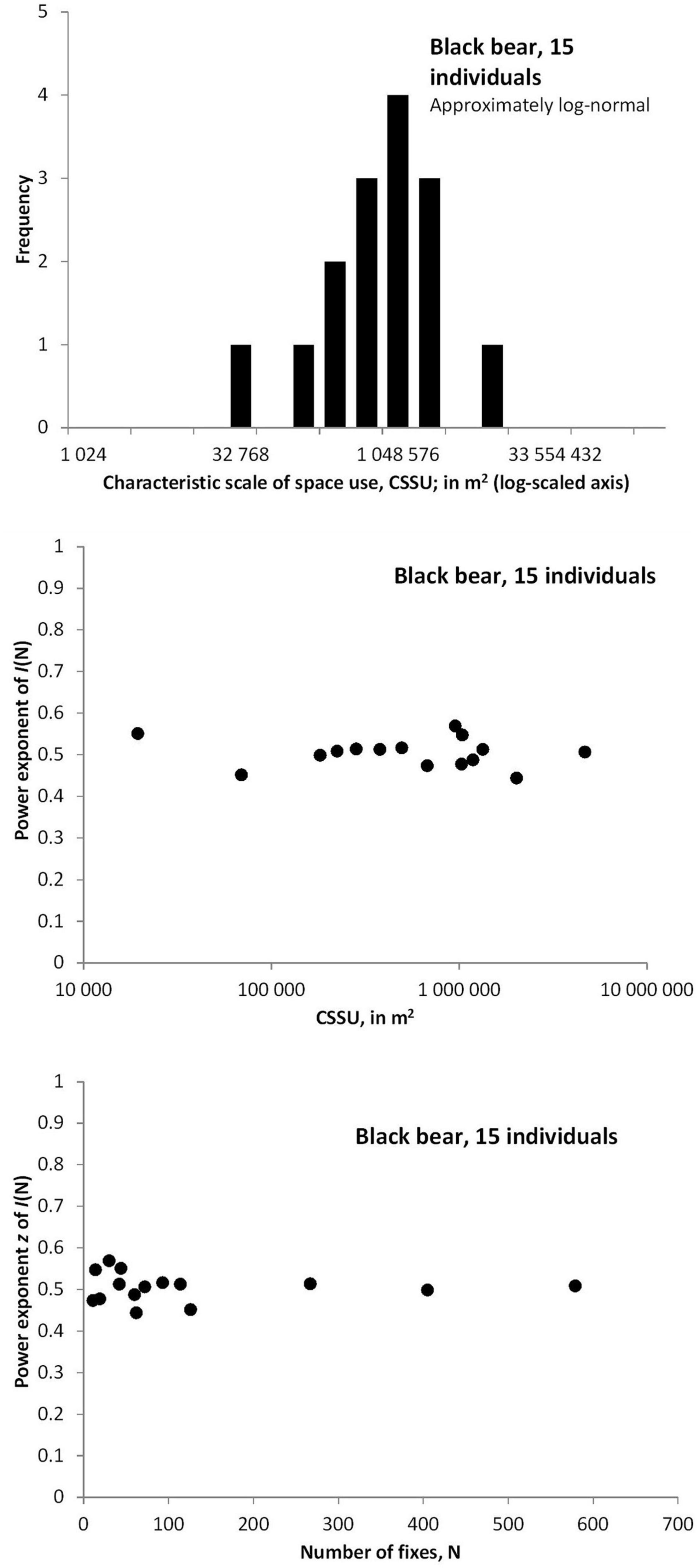
Figure 9. Upper pane: The CSSU estimates for the respective series varies strongly. Middle pane: z is independent of the parameter CSSU, and varies little between the series. Lower pane: z is independent also of fix sample size N, and varies little between the series.

Discussion

Network Topology in an Site Fidelity Network Context

With respect to ecological aspects of memory-influenced animal space use, the difference between a complex and a regular network topology may have substantial influence on the organic growth and stability of site fidelity. In general, a scale-free network topology is expected to show a high resilience against perturbations. For example, the hierarchical distribution of routers and inter-domain connectivity of the World Wide Web is expected to communicate unaffectedly even when experiencing unrealistic high failure rates given that the errors are randomly distributed among the nodes (Albert et al., 2002). On the other hand, if the dominant nodes have a higher degree of failure than expected from random shutdown both the network resilience and its hierarchical structure easily breaks down (Albert et al., 2002). Under such events the most popular nodes are being specifically attacked rather than being subject to random error on equal terms with other nodes. Hence, scale-free networks have an Achilles heel, which may counter-balance the general advantages from hierarchical system topology: robustness from such organization of nodes makes the structure vulnerable if the dominant nodes are specifically targeted and destroyed.

Returning from the general network theory above and back to ecology, if the nodes that are utilized most intensely are destroyed, the consequence should be expected to be more severe than expected from their node degree alone; i.e., the percent use of given nodes relative to all nodes’ degree, where degree is synonymous with relative popularity. However, under SFN terms, which represent a non-classic variant of complex networks, disruptions may have both external and internal causes. In the latter case, consider an animal that (gradually or more abruptly) for ecological reasons is choosing to abandon its present set of preferred patches in total or in part, for example due to intra-seasonal habitat phenology or other changes of space use. This kind of shifting mosaic of site fidelity takes place (under the premise of the MRW model) at many temporal scales in parallel, and represents an important aspect of cognitive movement ecology to be explored. Thus, SFN introduces a qualitatively different kind of resilience against perturbations than expected from premises of a classic, scale-free network.

First of all it is interesting that a scale-free kind of node hierarchy (the degree distribution) is found under memory utilization and site fidelity, but not necessarily depending on the MRW scale-free properties of the MRW model [the spatially explicit step length distribution and the I(N) function]. Space use complexity in terms of network topology might thus be expected over a very broad range of environmental conditions and cognitive processing of spatio-temporal memory, given that the actual animal complies with site fidelity. What about space use vulnerability to perturbations? Animals that use spatial memory to revisit patches in a self-reinforcing manner may as a side-effect also develop resilience against destruction of even a large percentage of its revisited patches. Like the stream of data over the Internet, the traffic simply finds alternative routes and—over time—swiftly absorbs the perturbations by developing alternative nodes and links, including shortcuts.

In ecological terms, nodes may represent localized food items or food-rich localities, which may occasionally be temporally destroyed or made less attractive either by the individual’s foraging activity or by competitors. A range of other external factors may also reduce the assumed profit from returning to a given locality, in the shorter or longer term. If resource availability generally becomes less abundant, site fidelity and the emerging scaling property of space use may even break down, as illustrated by simulations (Gautestad and Mysterud, 2010b). Thus, under a combination of general resource depletion and disruption of resource patches (self-inflicted or not), the animal may drift (or swiftly move) toward other localities and develop a modified space use network. The present results indicate how the degree of site fidelity, from resilience to drifting or re-building, may be studied in the I(N) function with respect to the difference between the two sampling schemes for varying N. Stronger degree of shifting mosaic of utilized patches is expected to show a wider gap between the two scheme results of I(N) relative to the log-log line for their geometric mean.

In terms of fitness, a self-reinforcing feedback type of patch use may lead to fine-scaled habitat auto-facilitation (Gautestad and Mysterud, 2010b). Habitat facilitation is normally a descriptor of how a keystone species may facilitate the habitat for other species (Arsenault and Owen-smith, 2002; Fox et al., 2003; Liess and Helmut, 2004; Korpinen et al., 2008; Pringle, 2008). However, a species like a grazing ungulate may also auto-facilitate—self-facilitate—a given habitat in a self-reinforcing manner, and thereby improve or maintain the local habitat’s grazing potential for a given individual, family group, herd or local population. Mild grazing, i.e., below or at an optimum intensity of patch use, may induce a higher re-growth rate and/or maintain a high level of digestibility for some important food plants (Mobæk et al., 2009).

However, as the utilization rate increases a critical threshold is always lurking. The positive feedback may then switch into a negative feedback, at least until the patches may be restored with respect to their attractive attributes (Gautestad and Mysterud, 2010b). The development of a network of nodes as a consequence of site fidelity is a two-edged sword also from other reasons: by becoming increasingly attached to the most utilized super-nodes (Figure 3) the animal may simultaneously make itself vulnerable. For example, predators may learn where these nodes are located, and gradually adapt their search behavior accordingly. The present simulations may thus open new and interesting directions of research, based on the various complex aspects that are successively revealed in a Russian doll manner on the interface between virtual network theory and animal ecology.

Network Topology in Relation to Local Density of Fixes

The distribution of node degree (connectedness) in the oldest part of the Site Fidelity Network (SFN) does not comply with expectation from a regular (non-complex) network system, but resembles a complex (hierarchically structured) space use over a wide range of connectivity conditions. Another interesting aspect of the present analyses regards the absence of a clear correlation between spatial locations of the dominating nodes from the virtual network space—“super-nodes”—relative to the areas of most intense use. The latter regards the nodes of the more traditionally considered utilization distribution, which is based on local density of fixes (for example, core areas from multi-modal kernel density estimates). In contrast, under MRW the local density modality emerges as a multi-scale mixture of network node locations and dispersion of exploratory moves.

The unexpected result in Figure 3 regarding distribution of “super-nodes” opens for interesting speculations with respect to cognitive movement ecology and animal space use in general: even if a spatial grid cell containing a super-node contains a low local density of relocations relative to many other parts of the animal’s home range, the actual super-node may represent a locality with stronger importance than revealed by the traditional utilization distribution alone. However, even if the overview of complex network properties in Introduction referred to a network’s susceptibility to perturbations of the most visited nodes, one may speculate that an animal’s network of site fidelity may show stronger resilience overall, due to spatial memory. If a super-node is destroyed of abandoned, the individual may take advantage of shifting to an alternative location in the understory of potential nodes in the hierarchy of historically utilized and remembered locations. In this respect the presently described SFN, due to its large set of potential nodes, deviates qualitatively from more traditional network theory, whether complex or regular. Thus, ecological inference with respect to analysis of space use under condition of site fidelity should take both the Euclidean and the virtual network topology into consideration.

While the set of network nodes is small relative to the large majority of locations that are revisited only 0–1 times, resilience of nodes determines both the emergence of a “home range” and its degree of spatial stability. The present results show that the super-nodes may be surprisingly uncorrelated with a home range’s core areas, which reflect the utilization distributional peaks; i.e., the spatial density of relocations of an individual. Thus, a maturing network of habitat utilization may to a large extent be determined by the non-trivial dispersion of the rich understory of less frequently visited nodes relative to the most visited ones.

In this respect the local “peaks” that are represented by the location of the super-nodes in Figure 3A will typically go undetected in a standard Kernel Density Estimate function, which is “smoothing” the utilization distribution under the statistical premise that the underlying space use process complies with diffusion-like, scale-specific dynamics in statistical-physical terms; i.e., the distribution may under this condition be represented by a multi-modal function of a superposition of many normal distributions, which then are implicitly expected to reflect environmental heterogeneity. The node peaks in Figure 3A will thus easily become “averaged away” due to applying an erroneous biophysical framework for the analysis. On the other hand, the super-nodes are also undetectable by direct visual inspection, as illustrated by the complex dispersion of fixes in Figure 3A. This aspect of the MRW model underscores the importance of studying local space use intensity from variation in CSSU rather than studying the local density of fixes directly.

The SFN model may point toward exploring a novel aspect of animal space use where conditions for site fidelity are satisfied, by showing how the physical (Euclidean) and the virtual network of nodes and links represent complementary aspects of memory-influenced movement. Specific aspects and properties may even be uncorrelated between these representations. The theory of network topology may thus spin off new and unexplored hypotheses, which in a fruitful development in tandem with ecological field experiments may give further insight with respect to the dynamics of animal space use and dispersal. For example, the vulnerability to surgical node destruction in combination with the present insight that these nodes may be uncorrelated with a home range’s primary core areas (Figure 3) may lead to modified protocols with respect to protection of wildlife. It may also provide guidelines for the opposite: more effective destruction of the conditions for local persistence of pest species.

Drifting Site Fidelity

In sum, the present simulation conditions for drifting fidelity cover a wide range of memory horizons. In parsimonious model terms, they thus cover a wide range of situations where the animal is utilizing a memory map during adaptation to a temporally shifting mosaic of habitat heterogeneity.

The similarity between the average log[I(N)] slopes with z close to 0.5 at the CSSU scale for all punctuation conditions under neutral connectivity indicates resilience both with respect to different percentage overlap of locations between successive time sections and various magnitude of these sections (Figure 4B). Thus, the difference between continuous-time and frequency-based sampling in the I(N) scatter plot (stronger divergence in the medium-N range) is due to the autocorrelation that follows from the drifting pattern of site fidelity. However, the result showing similar magnitude of both the power exponent z and the intercept c reflects stability with respect to how the individual distributed its space use over the range of scales, whether the site fidelity was stable of temporally variable during the given time span.

A condition of a partly retained site fidelity leads to a tendency for a “drifting home range” (Doncaster and Macdonald, 1991), with some degree of locking toward previous patch use, similar to the condition that was simulated and discussed in Gautestad and Mysterud (2006). Behaviorally, punctuated site fidelity illustrates an animal that is faithful to its environment in landscape-scale terms, but occasionally is developing partly new local habitat utilization as time progresses. For example, this scenario could in model-simplistic terms illustrate GPS sampling of an ungulate that occasionally is changing its space use in accordance to changing food distribution during the season (Gautestad and Mysterud, 2006; Bischof et al., 2012). Punctuated site fidelity could also illustrate an intrinsic predator avoidance strategy, whereby fitness may improve by occasional abrupt changes of patch use, and this may under specific conditions be more advantageous than the cost of occasionally giving up utilization of familiar patches. It could also illustrate patch deterioration with respect to a critical resource; energy profit in utilized patches may deteriorate owing to foraging, and thus trigger a “reset” of patch use in conceptual compliance to the marginal value theorem (Charnov, 1976).

Consequently, for wildlife management and conservation biology it should be of great importance to clarify whether individual space use under influence of spatial memory tends to follow the dynamic principles of scale-free or approximately scale-free (complex) or a scale-specific (non-complex) networks. Either way, the emergence of a network of actual and potential nodes requires that the animal is utilizing a memory map for occasional, non-random returns.

Model Feasibility

To my knowledge MRW is at present the only model developed explicitly for GPS relocation sampling scale that has been shown to reproduce three crucial statistical-physical aspects of individual space use with properties in accordance to our analyses of empirical GPS data (op. cit.); power law compliant and non-trivial sample size dependence on observed home range area I(N), power law distribution of step lengths F(L) and power law space use dispersion, as expressed by the fractal dimension D. Our results from empirical analyses have been coherent with theory developed for the relationship between these three aspects, based on the MRW properties (Gautestad and Mysterud, 2010a,b; Gautestad and Mysterud, 2013; Gautestad et al., 2013; Gautestad, 2021). In the present report we extend the MRW framework by studying a fourth aspect of the model; the topology of network nodes.

Owing to the return events, space use becomes very constrained relative to movement with no site fidelity. Consequently, the total energy expenditure for a return step is not expected to be substantially different on average from an exploratory step. Complications with respect to modeling energetic cost of short and long steps may thus be ignored in the present context (Figure 10), a property that is consistent with some recent empirical studies (Merkle et al., 2014; Marchand et al., 2017; Merkle et al., 2017). Thus, the energetic aspect lends additional weight to the feasibility of the MRW framework. Memory utilization is energy-efficient, relative to the standard space use paradigm, where the animal is implicitly assumed to obey the general statistical-physical principles of Markovian dynamics (see below).

FIGURE 10

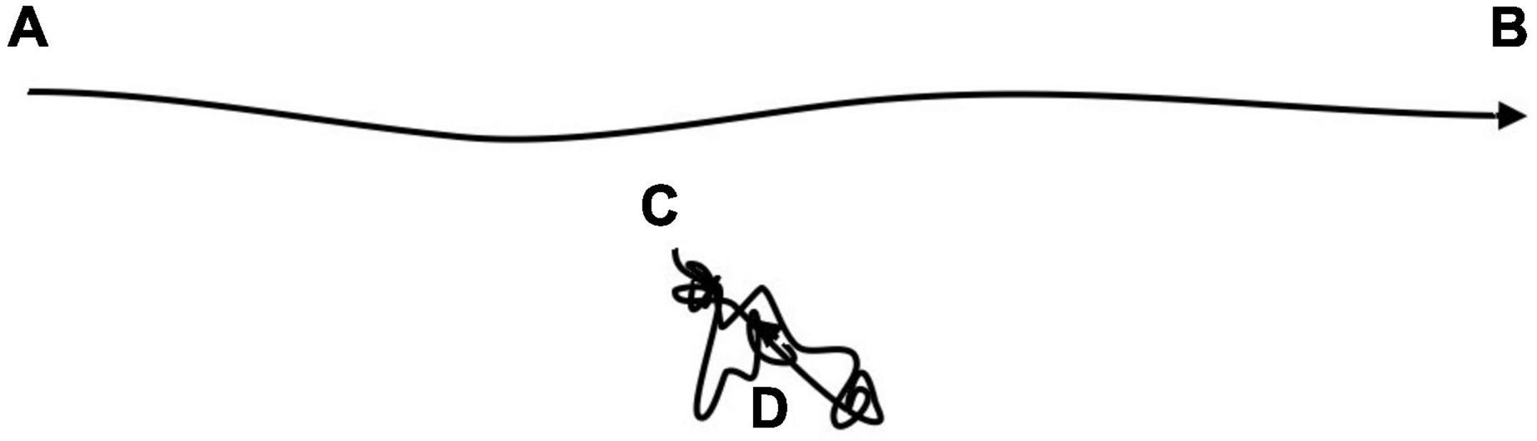
Figure 10. The movement path from fix locations A to B has the same total length as the path from locations C to D, but in the latter case the path includes return events, which curls the path. Since a location along the latter path has a relative short distance from any other location, the energy expenditure from returning to an old location (close to C) is of similar magnitude as revisiting a relatively recent location (close to D). Thus, in the present simulations return events take place without penalty from time since last visit to the target location.

It should be emphasized that MRW locations that are returned to regard exact geometric positions relative to their first occurrence in the series. However, the present results do not depend on such exact position. The crucial point is that each simulation makes an intrinsic distinction between true return targets (even if these are geometrically rounded to a coarser-defined site) and exploratory steps that just happen to land at a given previous site.

Regardless of strength of connectivity, since return steps in statistical terms may target any previously visited location irrespective of previous revisits, physical patch distances and virtual network distances are in this manner set to be independent a priori. The model choice to return to a randomly picked location under the given strength of connectivity may be considered consistent with general principles of statistical mechanics of movement in a homogeneous environment. Heterogeneity and deterministic behavior are under this approach implicitly confined to finer resolutions (for example, from varying local strength of site fidelity as a function of local habitat attributes, as expressed by a in Eq. 1), and averaged out in the distribution results from the complete set of fixes. This implicit fine-grained heterogeneity may thus be replaced by a homogeneous environmental property in the model for the sake of simplicity.

MRW builds on a non-mechanistic (non-Markovian) kind of statistical mechanics, as a consequence of implementation of memory as defined by the model’s premises of “parallel processing” rather than “serial processing” (Gautestad, 2021). In order to embed “non-mechanistic” processes, the framework of mechanical dynamics have been extended to allow for the originally “peculiar” aspects of animal movement, under which some specific paradoxes have been theoretically resolved. The MRW conjecture of non-Markovian processing rests on the memory property where returns happen independently of temporal interval since previous visit to a given location. This property makes the time domain scale-free: a given location has—on average—a geometrically declining probability for a revisit due to the maturing of space use over time (“longer path”). Simultaneously, multiplying this declining revisit probability to a given location with the number of potential nodes as a path is growing will compensate this decline. Thus, this product reflects a uniform (constant) next-step return probability pr. unit time.

From another perspective, the mechanistically unfamiliar MRW property of Eq. 2, where observed area expansion is a function of N rather than time as such, also violates a basic property of a mechanistically driven system. Adding new fixes may be performed in a time-incremental manner (continuous sampling; a sample size that is proportional with sampling time) or by increasing sampling frequency 1/t within the total time period T (including every n^th fix within T, by increasing n until n = N). This statistical-physical property, originally termed “The Home range Ghost” (Gautestad and Mysterud, 1995), makes the process time-independent (and thus non-mechanistic) but temporally scale-range dependent of the ratio T/t. In other words, a similar change of both T and 1/t gives a similar change of the expectancy of I(N) when averaging over the two sampling schemes. The present study lends additional empirical and simulation-based results in this respect; the power law in Eq. 2 not only regards serially non-autocorrelated sets of fixes, but—crucially and non-trivially—also autocorrelated sets. The latter regards the geometric averaging of continuous and frequency-based sampling, which (as shown in Figures 4–7) restores compliance with Eq. 2.

In contrast, in a Marovian system, a given return is a function of current or recent conditions (first- or n-order Markov, respectively). Thus, “infinite” memory influence on next-move decisions (the core of the parallel processing conjecture) is computationally dismissible. However, mechanistic implementation of memory-based site fidelity as alternatives to MRW has also been proposed and explored by others (Morales et al., 2005; Dalziel et al., 2008; van Moorter et al., 2009; Boyer and Walsh, 2010; Nabe-Nielsen et al., 2013; Boyer and Romo-Cruz, 2014; Boyer and Solis-Salas, 2014; Bracis et al., 2015). It will be interesting to see which of the two theoretical directions to understand the observations of complex movement as expressed by Eq. 2 gain further support in the time ahead; parallel processing under scale-extended statistical mechanics, or scale-specific (Markovian) processing under standard biophysical premises.

Characteristic Scale of Space Use: Expressing the Balance of Exploratory Moves, Return Frequency and Preferential Connectivity

In addition to exploring topological aspects of memory-influence in general terms, the second main part of this report reveals important properties of various degree of drifting site fidelity in the Euclidean realm. In particular, I describe how the divergence between I(N) from continuous and frequency-based sampling appear as a feasible method to reveal such instability of site fidelity. Crucially, under a given condition of connectivity strength, unit step length a and constant average return frequency t_ret, both c and z from the total series (Eq. 2) are on average similar to c and z that are estimated from each of the ten separate time sections (Figure 4B). This result holds even when estimating these parameters under subsections of a given section; i.e., by reducing N within an interval with absence of forced drift of site fidelity (not shown). This property follows from the model independence between c, z and N. Hence, when averaging over spatio-temporal heterogeneity, the results confirm that the overall property of c and z is maintained. Even when temporal heterogeneity is further increased within the same total time span by using 50 sections with 2% overlap of potential nodes for return step locations, the averaging of time-continuous and frequency-based sampling verifies the power law with a consistent slope and intercept (Figure 5B). The drift effect on site fidelity is most strongly increased when historic locations are abandoned at every punctuation event (Figure 6). However, this report also shows that CSSU, as expressed by c, is not only a function of unit step length a of exploratory steps and t_ret for return events, but also influenced by the strength of preferential connectivity. Stronger preference leads to smaller CSSU; i.e., a more condensed space use (Figure 7).

However, under a given node connectivity regime, despite the added complexity of space use under the punctuated site affinity, a similar magnitude of c and thus CSSU is found. This is a non-trivial and important statistical-physical result: averaging over spatial and temporal heterogeneity of space use shows a similar result with respect to estimating c. The parameter c is thus confirmed to be very resilient with respect to finer-scaled heterogeneity relative to the chosen scales in time and space for the analysis.

The general recognition of spatio-temporal memory as a crucial aspect of animal space use is currently forcing a rapid extension of the theoretical foundation of animal movement modeling, in particular for vertebrates. In the present report I have deepened our own multi-decennial quest in this regard, by drilling into the topology aspect of memory-based site fidelity and how early-phase return events to previously visited locations tend to lock habitat utilization into the emergence of a home range. Contrary to the classic paradigm, under the present MRW model the concept of home range size becomes imprecise, due to the intrinsic scaling property of the mixture of exploratory bouts and return events. Incidence, I(N), describes a power law under changing N, in violation of the traditional expectation of an asymptotic approach toward a stationary home range size with increasing N. Consequently, the Characteristic Scale of Space Use, CSSU, is for statistical fractal-compliant fix patterns here (as in our previous papers) advocated as an alternative expression for size; i.e., “area pr. square root of N” (Eq. 2) rather than area per se. Under the MRW framework, the instability of I(N) under a change of N is not a trivial function of small-sample error (as under the paradigmic assumptions of a home range utilization), but is the result of varying observation intensity on a given multi-scaled and non-Markovian space use process. Obviously, this statement needs further validation, both theoretically and not at least empirically.

Figure 7 shows that space use drifts toward becoming more fine-gained in unit-scale CSSU terms as connectivity drifts from neutral toward preferential. This is quite logical and to be expected a priori, since constraining returns to a subset of previously visited locations by necessity also increases the relative connectivity to early-phase emergence of nodes. Consequently, I(N) for a given N becomes more constrained relative to neutral connectivity conditions. However, the stability of z when shifting from neutral to preferential connectivity is perhaps more surprising and supports the broad versatility of the MRW model as a parsimonious model for memory-influenced habitat utilization.

Black Bear Data Under the I(N) Analysis

While the previously published analysis of black bear movement (Gautestad et al., 1998) applied Rescaled Range analysis (R/S) (Mandelbrot, 1983; Feder, 1988) to test for MRW compliance, the present result confirms a similar pattern under the I(N) method where continuous and frequency-based sampling are averaged. Most relevant for the present context, the separation of these two fix sampling schemes scatter plots indicate that on average these individuals expressed some (un-quantified) magnitude of drifting site fidelity. The present re-analysis of a sample of black bear telemetry series, albeit very limited and prone to statistical uncertainty, provides important support for several aspects of the MRW approach. First, this pilot study shows that the power law of N-dependence of observed space use (Eq. 2) holds when shifting from Rescaled Range analysis (Gautestad et al., 1998) to an I(N) analysis (Figure 8). Second, independence between key parameters of the MRW model are supported (Figure 9), and third, the present result invites to further explorations of the ecological aspect of drifting site fidelity using the method that has been presented here.

In general, when analyzing real data; as long as sampling rate of fixes, t_obs, is larger than the average return rate, t_ret, and the movement behavior satisfies MRW, neither z nor c are influenced. In real data, a verification of this property is thereby indirectly achieved by finding stability of both parameters in I(N) as grid scale k is “zoomed” over a scale range. Too small k leads to z > 0.5 (as described in Supplementary Material 1), and too large k leads to z < 0.5. Where z approximates 0.5, the actual k-scale squared gives an estimate of CSSU.

Conclusion

As always, scientific progress is achieved by the dual development of theory and empirical tests. In this report a specific model, MRW, is applied to propose a novel direction to explore the evolution of two complementary aspects of animal space use under memory influence, the topological property of network graphs and whether the simulation-revealed property of node popularity may be revealed indirectly by studying Euclidean dispersion of fixes. The latter approach depends in the MRW model, which embeds several testable predictions. These properties come under further scrutiny here, as a side-effect of exploring topological properties of spatial memory and spatio-temporal properties of drifting site fidelity. First, the modern view of home range as an emerging object from occasional returns to popular sites is gaining additional support. Traditionally, home range theory has been based on individuals that are expressing independent local returns within a spatially constrained area (e.g., demarcations due to physical borders or territorial behavior). For example, many statistical methods in tests of habitat selection rest on an assumption of random and non-intentional self-crossing of the animal’s path, leading to “re-discovery” of profitable sites (i.e., a Markovian process). Second, verification of a MRW-like fix pattern (for example, compliance with Eq. 2) both supports a cognitive capacity for long term utilization of a memory map, and also a specific statistical-physical class of movement: a mixture of scale-free movement in tandem with occasional returns. Third, an acceptance of MRW-like behavior in statistical-physical terms has as a consequence that local space use intensity should preferably be quantified by CSSU and not by local density of fixes. Thus, two sections of a home range may express different magnitude of CSSU, despite a similar magnitude of fix density; or vice versa. Fourth, empirical support for scale-free and memory-influenced movement means a new direction to study to what extent an animal is distributing its habitat utilization effort over a scale range. In Eq. 2, a power exponent close to 0.5 rather than close to zero implies that—in statistical and over-all terms—the effort has been quite evenly distributed over this spatial range. Further, empirical support for long term memory and return events quite independent of the time span since last visit gives weight to the hypothesis of scale-free habitat utilization also in the time domain. Fifth, the MRW framework lends support to the quest to scrutinize the biophysical aspect of movement, rather than just taking the classic assumptions of a mechanistic, Markovian-compliant kind of process as granted.

To conclude, under the present approach site fidelity from memory utilization under the MRW conjecture should either be tested using methods that are available for this purpose (Gautestad, 2012, 2021), or this kind of behavior could be applied as a premise for analysis of complex habitat utilization if sufficient empirical support has accumulated.

Data Availability Statement

The raw data supporting the conclusions of this article will be made available by the authors, without undue reservation.

Ethics Statement

Ethical review and approval was not required for the animal study because Pilot study regarding statistical analysis of previously published data (Gautestad et al., 1998).

Author Contributions

The author confirms being the sole contributor of this work and has approved it for publication.

Funding

Some parts of the development of the MRW model were supported by funding from Centre for Ecological and Evolutionary Synthesis (CEES), University of Oslo, during the period 2011–2013.

Conflict of Interest

The author declares that the research was conducted in the absence of any commercial or financial relationships that could be construed as a potential conflict of interest.

Publisher’s Note

All claims expressed in this article are solely those of the authors and do not necessarily represent those of their affiliated organizations, or those of the publisher, the editors and the reviewers. Any product that may be evaluated in this article, or claim that may be made by its manufacturer, is not guaranteed or endorsed by the publisher.

Acknowledgments

I thank Eliezer Gurarie and four referees for valuable comments and proposals for improvements of presentation.

Supplementary Material

The Supplementary Material for this article can be found online at: https://www.frontiersin.org/articles/10.3389/fevo.2022.695854/full#supplementary-material

Footnotes

1. ^ See, for example Marchand et al. (2017, p. 68): “The assumption that toads returning to a previous refuge choose one at random may seem unrealistic. Yet it fits the data better than two alternative models we tested, where the probability of return and/or the choice of refuge were distance-dependent.”
2. ^ The present simulations and analyses are performed under the MRW Simulator 2.0, developed by the author (www.gautestad.com).
3. ^ See Author’s blog post “Roe Deer Comply With the MRW Model,” dated August 11, 2020, at www.animalspaceuse.net.
4. ^ For details on the MRW model, visit www.animalspaceuse.net.
5. ^ See, for example, http://www.animalspaceuse.net/2017/12/statistical-mechanical-details-on-space.html

References

Albert, R., Jeong, H., and Barabási, A. L. (1999). Diameter of the world-wide web. Nature 401, doi: 10.1038/43601 130–131.

CrossRef Full Text | Google Scholar

Albert, R., Jeong, H., and Barabási, A. L. (2002). Error and attack tolerance of complex networks. Nature 406, doi: 10.1038/35019019 378–382.

PubMed Abstract | CrossRef Full Text | Google Scholar

Arsenault, R., and Owen-smith, N. (2002). Facilitation versus competition in grazing herbivore assemblages. Oikos 97, 313–318. doi: 10.1073/pnas.1503283112

PubMed Abstract | CrossRef Full Text | Google Scholar

Barabási, A.-L., and Albert, R. (1999). Emergence of scaling in random networks. Science 286, 509–512. doi: 10.1126/science.286.5439.509

PubMed Abstract | CrossRef Full Text | Google Scholar

Barabási, A.-L., Albert, R., and Jeong, H. (1999). Mean-field theory for scale-free random networks. Physica A 272, doi: 10.1016/S0378-4371(99)00291-5 173–187.

CrossRef Full Text | Google Scholar

Barabási, A.-L., Dezsö, Z., Ravasz, E., Yook, S.-H., and Oltvai, Z. (2003). “Scale-free and hierarchical structures in complex networks,” in Modeling of Complex Systems: 7th Granada Lectures, eds P. L. Garrido and J. Marro (College Park, MD: American Institute of Physics), 1–16.

Google Scholar

Barthélemy, M., Barrat, A., Pastor-Satorras, R., and Vespignani, A. (2004). Velocity and hierarchical spread of epidemic outbreaks in scale-free networks. arXiv [Preprint] arXiv:cond-mat/0311501v2 doi: 10.1103/PhysRevLett.92.178701

PubMed Abstract | CrossRef Full Text | Google Scholar

Bastian, M., Heymann, S., and Jackomy, M. (2009). “Gephi: an open source software for exploring and manipulating networks,” in Proceedings of the International AAAI Conference on Weblogs and Social Media (Menlo Park, CA: Association for the Advancement of Artificial Intelligence), 361–362.

Google Scholar

Bischof, R., Loe, L. E., Meisingset, E. L., Zimmermann, B., van Moorter, B., and Mysterud, A. (2012). A migratory northern ungulate in pursuit of spring: jumping or surfing the green wave? Am. Nat. 180, 407–424. doi: 10.1086/667590

PubMed Abstract | CrossRef Full Text | Google Scholar

Boyce, M. S., Vernier, P. R., Nielsen, S. E., and Schmiegelow, F. K. A. (2002). Evaluating resource selection functions. Ecol. Model. 157, 281–300.

Google Scholar

Boyer, D., Crofoot, M. C., and Walsh, P. D. (2012). Non-random walks in monkeys and humans. J. R. Soc. Interface 9, 842–847. doi: 10.1098/rsif.2011.0582

PubMed Abstract | CrossRef Full Text | Google Scholar

Boyer, D., and Romo-Cruz, J. C. R. (2014). Solvable random-walk model with memory and its relations with Markovian models of anomalous diffusion. Phys. Rev. E 90, 1–12. doi: 10.1103/PhysRevE.90.042136

PubMed Abstract | CrossRef Full Text | Google Scholar

Boyer, D., and Solis-Salas, C. (2014). Random walks with preferential relocations to places visited in the past and their application to biology. arXiv [Preprint] arXiv 1403.6069v1 doi: 10.1103/PhysRevLett.112.240601

PubMed Abstract | CrossRef Full Text | Google Scholar

Boyer, D., and Walsh, P. D. (2010). Modelling the mobility of living organisms in heterogeneous landscapes: does memory improve foraging success? Philos. Trans. R. Soc. A 368, 5645–5659. doi: 10.1098/rsta.2010.0275

PubMed Abstract | CrossRef Full Text | Google Scholar

Bracis, C., Gurarie, E., Van Moorter, B., and Goodwin, R. A. (2015). Memory effects on movement behavior in animal foraging. PLoS One 10:e0136057. doi: 10.1371/journal.pone.0136057

PubMed Abstract | CrossRef Full Text | Google Scholar

Broido, A. D., and Clauset, A. (2019). Scale-free networks are rare. Nat. Commun. 10, 1–10. doi: 10.1038/s41467-019-08746-5

PubMed Abstract | CrossRef Full Text | Google Scholar

Charnov, E. L. (1976). Optimal foraging: the marginal value theorem. Theor. Popul. Biol. 9, 129–136. doi: 10.1016/0040-5809(76)90040-X

CrossRef Full Text | Google Scholar

Dalziel, B. D., Morales, J. M., and Fryxell, J. M. (2008). Fitting probability distributions to animal movement trajectories: using artificial neural networks to link distance, resources and memory. Am. Nat. 172, 248–258. doi: 10.1086/589448

PubMed Abstract | CrossRef Full Text | Google Scholar

Doncaster, C. P., and Macdonald, D. W. (1991). Drifting territoriality in the red fox Vulpes vulpes. J. Anim. Ecol. 60, 423–439. doi: 10.2307/5288

CrossRef Full Text | Google Scholar

Evans, M. R., Majumdar, S. N., and Schehr, G. (2019). Stochastic resetting and applications. J. Phys. A Math. Theor. 53, 1–67. doi: 10.1088/1751-8121/ab7cfe

CrossRef Full Text | Google Scholar

Feder, J. (1988). Fractals. New York, NY: Plenum Press.

Google Scholar

Fox, B. J., Taylor, J. E., and Thompson, P. T. (2003). Experimental maipulation of habitat structure: a retrogresion of the smalll mammal succession. J. Anim. Ecol. 72, 927–940. doi: 10.1046/j.1365-2656.2003.00765.x

CrossRef Full Text | Google Scholar

Gautestad, A. O. (2012). Brownian motion or Lévy walk? Stepping towards an extended statistical mechanics for animal locomotion. J. R. Soc. Interface 9, 2332–2340. doi: 10.1098/rsif.2012.0059

PubMed Abstract | CrossRef Full Text | Google Scholar

Gautestad, A. O. (2015). Animal Space Use: Memory Effects, Scaling Complexity, and Biophysical Model Coherence. Indianapolis, IN: Dog Ear Publishing.

Google Scholar

Gautestad, A. O. (2021). Animal Space Use, Second Edition: Memory Effects, Scaling Complexity and Biophysical Model Coherence. Newcastle upon Tyne: Cambridge Scholars Publishing.

Google Scholar

Gautestad, A. O., Loe, L. E., and Mysterud, A. (2013). Inferring spatial memory and spatiotemporal scaling from GPS data: comparing red deer Cervus elaphus movements with simulation models. J. Anim. Ecol. 82, 572–586. doi: 10.1111/1365-2656.12027

PubMed Abstract | CrossRef Full Text | Google Scholar

Gautestad, A. O., and Mysterud, A. (2013). The Lévy flight foraging hypothesis: forgetting about memory may lead to false verification of Brownian motion. Mov. Ecol. 1, 1–18. doi: 10.1186/2051-3933-1-9

PubMed Abstract | CrossRef Full Text | Google Scholar

Gautestad, A. O., and Mysterud, I. (1993). Physical and biological mechanisms in animal movement processes. J. Appl. Ecol. 30, 523–535. doi: 10.2307/2404192

CrossRef Full Text | Google Scholar

Gautestad, A. O., and Mysterud, I. (1995). The home range ghost. Oikos 74, 195–204. doi: 10.2307/3545648

CrossRef Full Text | Google Scholar

Gautestad, A. O., and Mysterud, I. (2005). Intrinsic scaling complexity in animal dispersion and abundance. Am. Nat. 165, 44–55. doi: 10.1086/426673

PubMed Abstract | CrossRef Full Text | Google Scholar

Gautestad, A. O., and Mysterud, I. (2006). Complex animal distribution and abundance from memory-dependent kinetics. Ecol. Complex. 3, 44–55.

PubMed Abstract | Google Scholar

Gautestad, A. O., and Mysterud, I. (2010b). Spatial memory, habitat auto-facilitation and the emergence of fractal home range patterns. Ecol. Model. 221, 2741–2750. doi: 10.1016/j.ecolmodel.2010.08.014

CrossRef Full Text | Google Scholar

Gautestad, A. O., and Mysterud, I. (2010a). The home range fractal: from random walk to memory dependent space use. Ecol. Complex. 7, 458–470. doi: 10.1016/j.ecocom.2009.11.005

CrossRef Full Text | Google Scholar

Gautestad, A. O., and Mysterud, I. (2012). The dilution effect and the space fill effect: seeking to offset statistical artifacts when analyzing animal space use from telemetry fixes. Ecol. Complex. 9, 33–42. doi: 10.1016/j.ecocom.2011.11.005

CrossRef Full Text | Google Scholar

Gautestad, A. O., Mysterud, I., and Pelton, M. R. (1998). Complex movement and scale-free habitat use: testing the multi-scaled home range model on black bear telemetry data. Ursus 10, 219–234.

Google Scholar

Jeong, H., Tombor, B., Albert, R., Oltvai, Z., and Barabási, A.-L. (2000). The large-scale organization of metabolic networks. Nature 207, 651–654. doi: 10.1038/35036627

PubMed Abstract | CrossRef Full Text | Google Scholar

Korpinen, S., Jormalainen, V., and Ikonen, J. (2008). Selective consumption and facilitation by mesograzers in adult and colonizing macroalgal assemblages. Mar. Biol. 154, 787–794. doi: 10.1007/s00227-008-0971-6

CrossRef Full Text | Google Scholar

Liess, A., and Helmut, H. (2004). Invited review: direct and indirect effects in herbivore-periphyton interactions. Arch. Hydrobiol. 159, 433–453. doi: 10.1127/0003-9136/2004/0159-0433

CrossRef Full Text | Google Scholar

Mandelbrot, B. B. (1983). The Fractal Geometry of Nature. New York, NY: W. H. Freeman and Company.

Google Scholar

Marchand, P., Boenke, M., and Green, D. M. (2017). A stochastic movement model reproduces patterns of site fidelity and long-distance dispersal in a population of Fowler’s toads (Anaxyrus fowleri). Ecol. Model. 360, 63–69. doi: 10.1016/j.ecolmodel.2017.06.025

CrossRef Full Text | Google Scholar

Merkle, J. A., Fortin, D., and Morales, J. M. (2014). A memory-based foraging tactic reveals an adaptive mechanism for restricted space use. Ecol. Lett. 17, 924–931. doi: 10.1111/ele.12294

PubMed Abstract | CrossRef Full Text | Google Scholar

Merkle, J. A., Potts, J. R., and Fortin, D. (2017). Energy benefits and emergent space use patterns of an empirically parameterized model of memory-based patch selection. Oikos 126, 185–195. doi: 10.1111/oik.03356

CrossRef Full Text | Google Scholar

Mobæk, R., Mysterud, A., Loe, L. E., and Holand, Ø., and Austrheim, G. (2009). Density dependent and temporal variability in habitat selection by a large herbivore; an experimental approach. Oikos 118, 209–218. doi: 10.1111/j.1600-0706.2008.16935.x

CrossRef Full Text | Google Scholar

Morales, J. M., Fortin, D., Frair, J. L., and Merrill, E. H. (2005). Adaptive models for large herbivore movements in heterogeneous landscapes. Landsc. Ecol. 20, 301–316. doi: 10.1016/j.scitotenv.2020.144000

PubMed Abstract | CrossRef Full Text | Google Scholar

Nabe-Nielsen, J., Tougaard, J., Teilmann, J., Lucke, K., and Forckhammer, M. C. (2013). How a simple adaptive foraging strategy can lead to emergent home ranges and increased food intake. Oikos 122, 1307–1316. doi: 10.1111/j.1600-0706.2013.00069.x

CrossRef Full Text | Google Scholar

Pasukonis, A., Warrington, I., Ringler, M., and Hödl, W. (2014). Poison frogs rely on experience to find the way home in the rainforest. Biol. Lett. 10, 1–4. doi: 10.1098/rsbl.2014.0642

PubMed Abstract | CrossRef Full Text | Google Scholar

Piper, W. H. (2011). Making habitat selection more “familiar”: a review. Behav. Ecol. Sociobiol. 65, 1329–1351. doi: 10.1007/s00265-011-1195-1

CrossRef Full Text | Google Scholar

Pringle, R. M. (2008). Elephants as agents of habitat creation form small vertebrates at the patch scale. Ecology 89, 26–33. doi: 10.1890/07-0776.1

PubMed Abstract | CrossRef Full Text | Google Scholar

Ranc, N., Moorcroft, P. R., Whitney Hansen, K., Ossi, F., Sforna, T., Ferraro, E., et al. (2020). Preference and familiarity mediate spatial responses of a large herbivore to experimental manipulation of resource availability. Sci. Rep. 10:11946. doi: 10.1038/s41598-020-68046-7

PubMed Abstract | CrossRef Full Text | Google Scholar

Redner, S. (1998). How popular is your paper? An empirical study of the citation distribution. Eur. Phys. J. B Condens. Matter Complex Syst. 4, 131–134. doi: 10.1007/s100510050359

CrossRef Full Text | Google Scholar

Reynolds, A. M., and Rhodes, C. J. (2009). The Lévy flight paradigm: random search patterns and mechanisms. Ecology 90, 877–887. doi: 10.1890/08-0153.1

PubMed Abstract | CrossRef Full Text | Google Scholar

Shlesinger, M. F., Zaslavsky, G. M., and Klafter, J. (1993). Strange kinetics. Nature 363, 31–37. doi: 10.1038/363031a0

CrossRef Full Text | Google Scholar

Song, C., Qu, Z., Blumm, N., and Barabási, A. L. (2010). Limits of predictability in human mobility. Science 327, 1018–1021. doi: 10.1126/science.1177170

PubMed Abstract | CrossRef Full Text | Google Scholar

Strogatz, S. H. (2001). Exploring complex networks. Nature 410, 268–276. doi: 10.1038/35065725

PubMed Abstract | CrossRef Full Text | Google Scholar

Swihart, R. K., and Slade, N. A. (1985). Influence of sampling interval on estimates of home-range size. J. Range Manag. 49, 1019–1025.

Google Scholar

van Moorter, B., Visscher, D., Benhamou, S., Börger, L., Boyce, M. S., and Gaillard, J.-M. (2009). Memory keeps you at home: a mechanistic model for home range emergence. Oikos 118, 641–652. doi: 10.1111/j.1600-0706.2008.17003.x

CrossRef Full Text | Google Scholar

Watts, D. J., and Strogatz, S. H. (1998). Collective dynamics of ‘small-world’ networks. Nature 393, 440–442. doi: 10.1038/30918

PubMed Abstract | CrossRef Full Text | Google Scholar