 Nika Galic
 Amelie Schmolke
 Steven Bartell3
95% of researchers rate our articles as excellent or good
Learn more about the work of our research integrity team to safeguard the quality of each article we publish.
Find out more
ORIGINAL RESEARCH article
Front. Ecol. Evol. , 13 January 2023
Sec. Conservation and Restoration Ecology
Volume 10 - 2022 | https://doi.org/10.3389/fevo.2022.1075244
This article is part of the Research Topic Models in Conservation and Restoration Ecology View all 9 articles
Introduction: Habitat restoration aims at reinstating abiotic and biotic habitat conditions to support long-term species persistence and viability. This management practice is commonly part of recovery plans developed for species listed as threatened or endangered under the Endangered Species Act. The endangered Topeka shiner (Notropis topeka) inhabits off-channel habitats, such as oxbow lakes which are increasingly the focus of restoration, but the exact abiotic conditions conducive to its persistence in this habitat are not fully understood. In this study, a hybrid model consisting of an individual-based model of the Topeka shiner and an aquatic ecosystem model representing the oxbow habitat was applied to identify optimal environmental conditions for the persistence of Topeka shiner populations.
Materials and methods: Environmental conditions that correlated with Topeka shiner presence were gathered from published studies and included water temperature, turbidity, oxbow depth, light intensity (as a function of riparian vegetation presence), dissolved nitrogen, and dissolved phosphorus. Selected conditions were systematically varied in simulations and results were analyzed with a partial rank correlation method that quantifies the relative influence on model output from multiple factors.
Results: Conducted simulations identified water temperature, depth, and dissolved inorganic nitrogen to be the most influential for Topeka shiner population biomass and additional simulations were conducted exploring the magnitudes and directions of effects of these three factors. Water temperature had the largest positive impact on population biomass followed by oxbow depth and nitrogen reduction.
Discussion: We recommend that the three identified factors be further explored in a combination of empirical and modeling approaches to advise management for the endangered Topeka shiner. This study demonstrated how ecological models could inform recovery plans by identifying factors that enhance species persistence. Ultimately, models should support management practices that result in long-term population viability of listed species and could facilitate their timely delisting.
Habitat degradation, in quality and quantity, and loss are the main sources of biodiversity declines (Brooks et al., 2002; Fahrig, 2003; Groom et al., 2006) and legal protections are provided in many countries for those species which are experiencing its negative effects. In the US, species are listed as threatened or endangered (T&E) under the Endangered Species Act (ESA) when their viability is jeopardized due to various reasons, including, e.g., environmental degradation, overexploitation, and invasive species. Once listed, recovery plans are developed that aim at improving the species status via various management strategies (Schwartz, 2008). For instance, agricultural activities, including modifications to naturally flowing streams (e.g., straightening of channels) have resulted in declines in many fish species occurring in the Midwest, including the Topeka shiner, Notropis topeka. This small cyprinid fish inhabits streams, oxbows, and other off-channel habitats in six states of the Great Plains and has been in decline due to the widespread modifications of prairie stream hydrology (U.S. Fish and Wildlife Service, 2018). The species was listed as endangered in Tabor (1998) and has since been the focus of concerted recovery efforts (U.S. Fish and Wildlife Service, 2019). The recovery vision for the Topeka shiner aims at multiple resilient groups of populations distributed across the species’ range which includes watersheds in Missouri, Kansas, and Iowa (U.S. Fish and Wildlife Service, 2019). The recommended recovery strategies include improving population size and viability via habitat restoration, oxbows habitat restoration, and floodplain connectivity.
Habitat restoration, as a common management practice, aims at reinstating habitat abiotic and biotic conditions conducive to the recovery of focal species or communities. Restoring oxbow lakes consists of dredging soils and sediments to reconnect the lakes with groundwater sources to provide sufficient water resources to support fish communities (Werblow, 2019). A number of oxbow restoration efforts have been undertaken in the Midwest in the last decade, but detailed information about their use by listed and non-listed species has thus far been relatively limited. A recent study analyzed both restored and unrestored oxbows for the presence of the Topeka shiner and fish assemblages to determine the abiotic and biotic factors that might support populations of this listed species (Simpson et al., 2019). Topeka shiners were consistently found in restored oxbows and the species’ presence was positively correlated with the presence of brassy minnows (Hybognathus hankisoni) and orange spotted sunfish (Lepomis humilis). Preference of Topeka shiners to be associated with the orange spotted sunfish is well known as the shiners spawn over sunfish’ nests and depend on male sunfish to guard and oxygenate the Topeka shiner eggs (Campbell et al., 2016). From abiotic factors only oxbow length (negative) and turbidity (positive) had a significant correlation with Topeka shiner presence. This study indicated that overall abiotic factors played a lesser role than the presence of certain fish species, but the authors noted the sampling limitations of abiotic factors. Constructing experimental oxbows was recommended to better test abiotic conditions to identify those combinations that increase the probability of Topeka shiner presence (Simpson et al., 2019). However, such an undertaking could prove to be logistically challenging and resource intensive if multiple combinations of factors were to be tested.
Ecological modeling could support listed species recovery management by identifying combinations of abiotic parameters that are most likely to support the presence and populations of focal species, such as the Topeka shiner. By systematically varying relevant parameters and their combinations, modeling may narrow the parameter ranges or identify combinations that could further be tested in the field. By ecological models, we refer to those models, mathematical or simulation, that incorporate biological, ecological, and other species characteristics and relevant processes to capture dynamics of individuals, populations, or ecosystems. To address recovery plans of many listed species, different types of models have been adopted and applied to identify those management scenarios that increase population persistence of listed species. For instance, a spatially-explicit individual-based model representing the endangered Greater Sage Grouse (Centrocercus urophasianus) was applied to compare several population recovery strategies (Heinrichs et al., 2018). In another study, a spatially-structured model was applied to assess population growth and extinction probabilities of the piping plovers (Charadrius melodus), a species listed as threatened under the ESA (McGowan et al., 2014). These and other studies focus primarily on analyzing demographic data and assumptions to estimate best management practices, but none have systematically analyzed possible environmental conditions that influence population persistence and abundance. Such information could prove to be invaluable in advising and supporting appropriate restoration practices.
This simulation study was conducted to identify combinations of environmental conditions that support the persistence of the listed Topeka shiner populations. It directly builds on a comprehensive study exploring abiotic and biotic factors driving Topeka shiner presence in oxbow habitats which suggests a more systematic exploration of abiotic factors is needed (Simpson et al., 2019). Even though the outcomes regarding the relevance of environmental conditions for the presence of Topeka shiner populations are generally inconclusive, this and other studies identified factors shown to influence its presence in oxbow habitats, including water temperatures, water turbidity, depth, and amount of riparian vegetation. Simulations were conducted with a previously developed and tested hybrid model consisting of a population model of the listed Topeka shiner and an aquatic ecosystem model, the latter providing the food web and fish assemblage context for the listed species (Bartell et al., 2019; Schmolke et al., 2019). Furthermore, given the potential of oxbow lakes to act as buffers for nutrient input into the streams and rivers, a range of nitrogen and phosphorus scenarios to determine their potential impacts on Topeka shiner populations was also simulated. Relevant abiotic factors were simulated in different combinations to identify those that have the largest influence on the biomass of Topeka shiner populations. The most relevant factors were then further analyzed in more detail.
The model applied in this study has been previously developed (Schmolke et al., 2019) and applied to assess risks to the listed Topeka shiner and its food web from exposure to the herbicide atrazine (Bartell et al., 2019) and the fungicide benzovindiflupyr (Schmolke et al., 2021). Briefly, this hybrid model consists of two separate models: (1) an individual-based model of the listed Topeka shiner (TS-IBM), and (2) an aquatic ecosystem model, i.e., the Comprehensive Aquatic System Model, adapted to represent off-channel (OC) habitats, i.e., Topeka shiner habitats (CASMOC) (Schmolke et al., 2021). The two models can be linked in two distinct ways: either directly by daily biomass exchanges between the models or with CASM providing daily inputs of prey biomass to the Topeka shiner IBM. The former allows for feedbacks between the two models; however, previous analyses demonstrate that the influence of Topeka shiners on their food web is negligible (Schmolke et al., 2019). In this study, therefore, we apply the latter linkage, where CASMOC provides an input file with a daily biomass of all prey items in the modeled food web to the Topeka shiner IBM (Figure 1). The full hybrid model documentation can be found in Schmolke et al. (2021).1
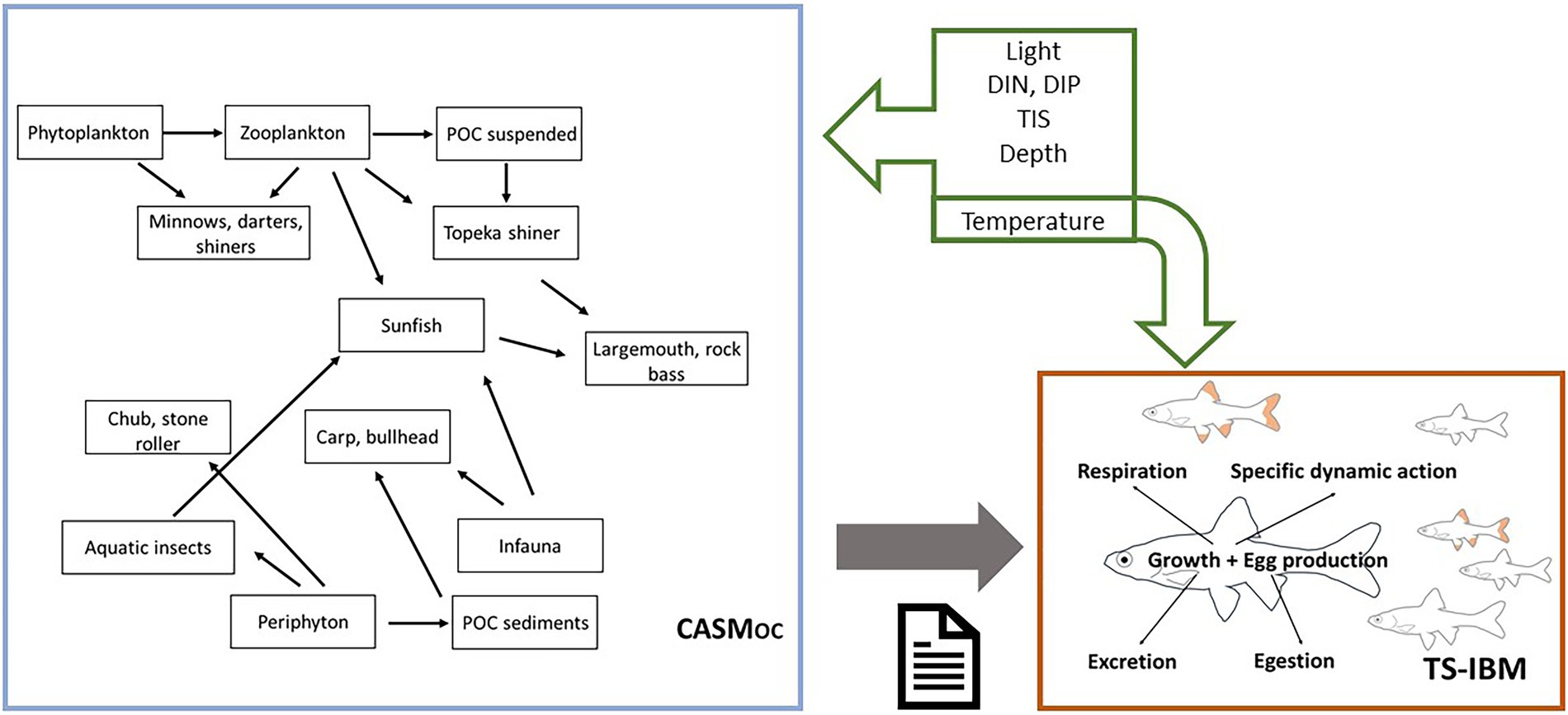
Figure 1. Representation of the hybrid model, consisting of the off-channel (oxbow lake) ecosystem model, CASMOC, and the Topeka shiner population model, TS-IBM. Figure based on Schmolke et al. (2019). CASMOC provides daily biomasses of various prey items that are consumed by Topeka shiner individuals simulated with the TS-IBM; only the key trophic linkages are indicated. Multiple abiotic factors (green arrows) drive processes in the CASMOC, whereas only temperature directly influences processes in the TS-IBM.
The Topeka shiner IBM represents each fish individually and follows individuals through their life cycle consisting of an egg, a larva, a juvenile, a subadult, and an adult stage. The growth and development of the simulated fish are based on the physiological rules outlined in the Wisconsin fish bioenergetics model (Hanson et al., 1997; Deslauriers et al., 2017). Here the food that is consumed is used to cover the costs of respiration and specific dynamic action (i.e., digestive processes), a fraction is lost via egestion and excretion, whereas the leftover energy is used for growth and reproduction (Figure 1). Both consumption and respiration are temperature dependent. Consumption is also dependent on prey availability and preference, as well as assimilation and handling efficiencies. Based on several studies examining the gut content of Topeka shiner (Dahle, 2001; Hatch and Besaw, 2001; Kerns and Bonneau, 2002), the simulated adults were assumed to feed on detritus, periphyton, Cladocera (combined with Ostracoda), Diptera (specifically midges), Ephemeroptera and Trichoptera (the latter summarizing several insect groups). Simulated juveniles start feeding on detritus and smaller organisms (microzooplankton, Rotifera, Copepoda, Cladocera, and Ostracoda). Once they reach the size of subadults, they switch to the adult diet. Start of reproduction is assumed once the fish reach a threshold length. The number of eggs produced is body size-dependent with larger females producing relatively more eggs.
The model version used in this study is the same as the one originally reported in Schmolke et al. (2019), with one exception. In the original version of the Topeka shiner IBM (Schmolke et al., 2019), parameters from the fathead minnow (Pimephales promelas) were applied to represent the bioenergetics and thermal preferences of the listed Topeka shiner (Hanson et al., 1997; Deslauriers et al., 2017). As no bioenergetics data were available for Topeka shiner, fathead minnow was chosen as surrogate because (a) the species is commonly observed as part of the species community including Topeka shiner, suggesting generally similar climatic and habitat preferences (Bakevich et al., 2013); (b) fathead minnow and Topeka shiner are related species, belonging to the family Leuciscidae (previously belonging to Cyprinidae) and are comparable in size and life span. This study explored the effects of environmental factors, including temperature, on the simulated Topeka shiner populations. Implementing a more realistic representation of the thermal preferences of Topeka shiner was important because temperature is a major driver of all bioenergetic processes and thus, population growth. For a more realistic representation of temperature preferences by Topeka shiner in the model, the fish bioenergetics model was fitted to experimental data reported by Koehle (2006), Koehle and Adelman (2007). In a series of experiments, growth of adult Topeka shiners under a range of temperatures was recorded. The total of six parameters driving the temperature dependence of consumption (four) and respiration (two) in the bioenergetics model were calibrated on growth data from this study. As the experimental study was conducted on adult organisms, possible life-stage differences in temperature preferences could not be derived and thus it was assumed that all life stages respond to temperature changes following the same function. All other parameters remained unchanged from the original model. The new parameter set for thermal dependency of consumption and respiration resulted in a narrower response to the thermal gradient than what was originally implemented using parameters from Deslauriers et al. (2017) for the fathead minnow. More detail on this analysis can be found in Schmolke et al. (2021).
The various prey items consumed by the Topeka shiner are provided by CASM that simulates daily biomass of a number of taxonomic groups, including both primary producers and consumers (Bartell et al., 2013, 2020; Schmolke et al., 2019). The CASMOC consists specifically of a food web that represents species in off-channel (e.g., oxbow) environments, as well as corresponding trophic interactions, and environmental input data representative of a generalized Iowa oxbow ecosystem (Schmolke et al., 2021). Primary producers include multiple populations of phytoplankton, periphyton, and macrophytes described by biomass growth equations consisting of photosynthesis-driven growth and catabolic and grazing biomass losses. Photosynthesis is driven by light, temperature, and nutrient (nitrogen, phosphorus, silica) availability. The consumer community consists of zooplankton, macroinvertebrates, and several fish species. Similarly, to primary producers, biomass dynamics of all consumer groups are functions of consumption and losses from respiration, excretion, natural (background) mortality, and predation. Consumption and respiration rates are temperature-dependent, while consumption is also dependent on prey biomass. As in the Topeka shiner IBM, grazing and predator–prey interactions are functions of prey availability and preference, assimilation, and handling efficiency.
The selection of relevant CASMOC species was based on relative abundance data reported for Iowa and Minnesota oxbows (Bakevich et al., 2013; Bybel et al., 2019). Species that were shown to be consistently present with the Topeka shiner were assumed to be a part of the “oxbow assemblage” (Figure 1). For instance, the golden redhorse Moxostoma erythrurum, the orange-spotted sunfish Lepomis humilis, central stoneroller Campostoma anomalum, and the black bullhead Ameiurus melas were selected because they were consistently found with Topeka shiners. Selecting fish species for an “oxbow assemblage” also considered the overall ecology of these systems. A balance among fishes in different trophic guilds was required (e.g., planktivores, omnivores, piscivores): the assemblage should not be all minnows and/or shiners. Therefore, the largemouth bass Micropterus salmoides was included, as well as rock bass Ambloplites rupestris which was included because of its diet breadth (i.e., insects, crustaceans, smaller fish). The CASMOC aquatic invertebrate food web also includes individual populations of ostracods (one of the zooplankton populations), corixids (water boatman), and coleopterans (water beetles) – these organisms are common to oxbows and other off-channel habitats. More detail about the relevant species selection process can be found in Schmolke et al. (2021).
The CASMOC represented an Iowa oxbow as 75 m × 15 m homogeneous system, with a constant daily water depth (~1.2 m). Environmental factors that influence population production in the CASMOC food web included daily values of surface light intensity, water temperature, water depth, current velocity, dissolved oxygen, nutrient concentrations (N, P, Si), concentrations of dissolved and particulate organic carbon (DOC, POC), and suspended inorganic sediments. Input values were based on data relevant to reconstructed Iowa oxbow off-channel habitats and Midwestern off-channel aquatic habitats (Kalkhoff et al., 2016).
The CASMOC calibration was based on: (1) derivation of initial fish biomass values and adjustment of fish bioenergetics parameters to achieve reported fish population biomass values for Iowa oxbows (Bakevich et al., 2013), (2) implementation of density-dependent fish growth and resetting initial biomass values for aquatic plants and invertebrates to produce stable population sizes across multiple years throughout the CASMOC food web, and (3) adjustments to bioenergetics parameters for phytoplankton, periphyton, zooplankton, and benthic invertebrates to generate biomass values for these guilds that were consistent with supporting modeled fish biomass. The calibration was guided in part by data provided in Bakevich et al. (2013) for fish, as well as estimates for zooplankton and benthic macroinvertebrate abundances based on numbers commonly encountered in similar freshwater systems.
The hybrid model was applied in a series of simulations aiming to determine combinations of environmental factors driving persistence of simulated Topeka shiner populations.
Environmental factors potentially indicative for the oxbow (off-channel) habitat quality for Topeka shiner were compiled from the literature. Habitat characteristics analyzed in the literature for correlation with Topeka shiner presence (or absence) included the substrate found at the bottom of the water body (Minckley and Cross, 1959; Kuitunen, 2001; Gerken and Paukert, 2013; Nagle, 2014; Campbell et al., 2016; Simpson et al., 2019), the aquatic and riparian vegetation (Minckley and Cross, 1959; Bayless et al., 2003; Bakevich et al., 2013; Simpson et al., 2019), land cover composition of the landscape surrounding the waterbody (Schrank et al., 2001; Wall et al., 2004; Gerken and Paukert, 2013; Prentice, 2013), water conductivity (Simpson et al., 2019), water pH (Bayless et al., 2003; Simpson et al., 2019), water temperature (Minckley and Cross, 1959; Simpson et al., 2019), water turbidity (Minckley and Cross, 1959; Kuitunen, 2001; Simpson et al., 2019), water depth (Fischer et al., 2018), and fish species community (Minckley and Cross, 1959; Schrank et al., 2001; Stark et al., 2002; Winston, 2002; Bayless et al., 2003; Bakevich et al., 2013; Gerken and Paukert, 2013; Campbell et al., 2016). From these factors, substrate, aquatic vegetation, land cover composition, water conductivity and pH, and the fish community composition were excluded from the simulations with the hybrid model. The riparian vegetation was included in the simulations indirectly by shading, i.e., reduction in the light intensity reaching the surface of the waterbody due to tree canopy which was found to be negatively correlated with Topeka shiner presence (Simpson et al., 2019). Substrate was identified as important by multiple studies but the kind of substrate reported to be preferred by Topeka shiner varied between studies (Minckley and Cross, 1959; Kuitunen, 2001; Gerken and Paukert, 2013; Nagle, 2014; Campbell et al., 2016; Simpson et al., 2019).
The hybrid model does not currently have the capability to simulate substrate explicitly, and the interactions with Topeka shiner or the food web are unclear. Aquatic vegetation (macrophyte cover) was not strongly correlated with Topeka shiner presence in published studies and the direction of the correlation was inconclusive among studies (Bakevich et al., 2013; Simpson et al., 2019). Terrestrial land cover around the aquatic habitat was excluded because it is not simulated by the model. Water conductivity is also not captured by the model. Water pH is simulated by CASMOC but was not included in the simulations because the two studies looking into pH indicated opposite associations of pH with Topeka shiner presence. Associations of Topeka shiner presence with the presence or absence of specific fish species was also inconclusive across studies (Minckley and Cross, 1959; Schrank et al., 2001; Stark et al., 2002; Winston, 2002; Bayless et al., 2003; Bakevich et al., 2013; Gerken and Paukert, 2013; Campbell et al., 2016). Due to the limited information about each of the fish species, the fish community was not tested as an environmental factor in the simulations. Finally, the model did not account for direct predatory pressures on the Topeka shiner because (1) species presence did not correlate with the presence of its predators (Simpson et al., 2019), (2) previous modeling study confirmed that direct predatory interactions result in population extirpation (Schmolke et al., 2019).
The environmental factors tested in the simulations are listed in Table 1. The reported correlations between these factors and Topeka shiner presence were not all consistent across studies, including turbidity and water temperature. For instance, water temperature has been found to be positively correlated with Topeka shiner presence in the study by Simpson (2018), but several older studies report positive correlation with cooler waters (Minckley and Cross, 1959; Mammoliti, 2002). Water turbidity was mostly reported as negatively correlated with Topeka shiner occurrence (Minckley and Cross, 1959; Kuitunen, 2001). Only one study reported that Topeka shiners prefer more turbid waters, but this was assigned to possible increased sampling efficiency (Simpson et al., 2019). Water depth was found to have no (Simpson et al., 2019) or mixed influences on Topeka shiner occurrence, but there was an overall preference for shallower oxbows (Ceas and Larson, 2010; Bakevich, 2012; Fischer et al., 2018). Simpson et al. (2019) found that the presence of woody riparian vegetation was negatively correlated to the Topeka shiner presence (Simpson et al., 2019), while non-woody vegetation had a positive impact on occurrence (Bayless et al., 2003; Simpson et al., 2019). The proximity of agricultural fields to many oxbows may result in increased nutrient input (Dubrovsky et al., 2010). Oxbows are even considered as potential nutrient-management strategy to reduce nutrient loading to streams (Kalkhoff et al., 2016). For this reason, nutrient loading was included to establish whether it may influence simulated population persistence, even though there were no studies correlating it with Topeka shiner occurrence.
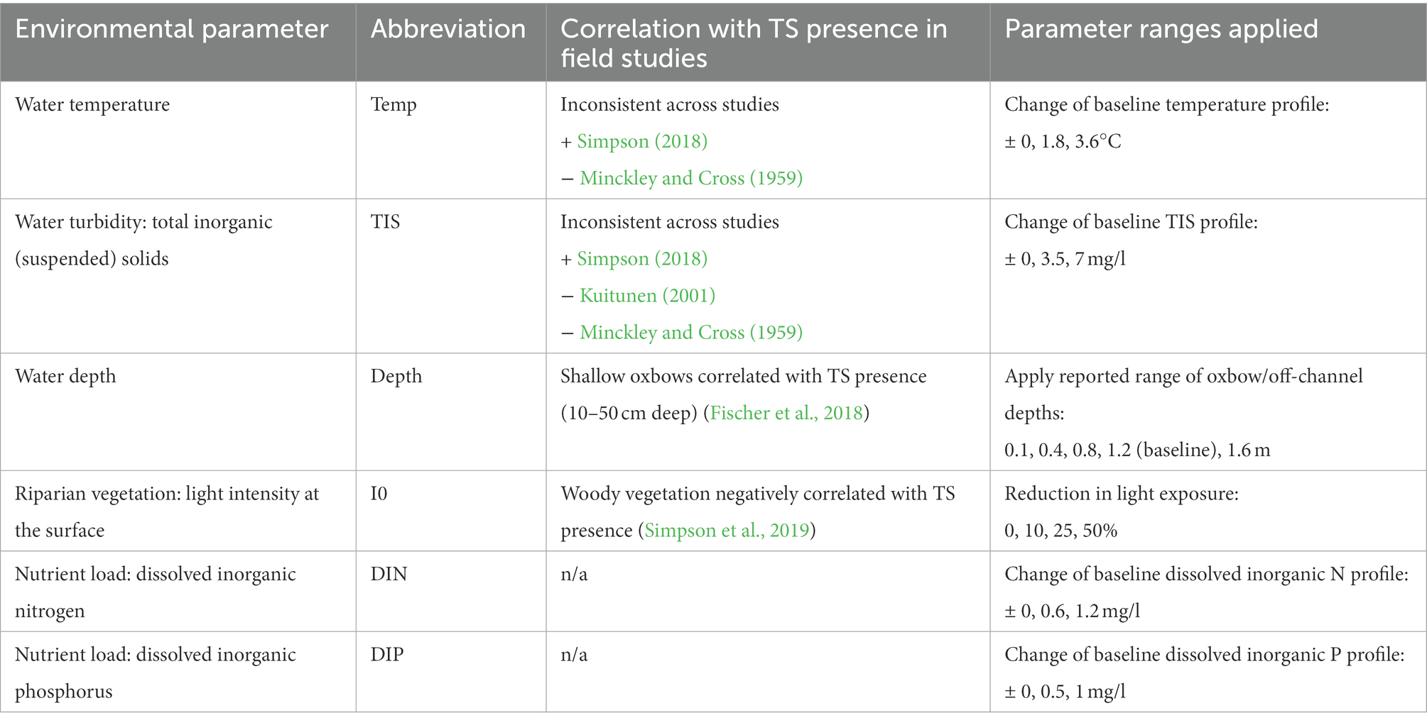
Table 1. Environmental parameters and their ranges used for simulations in the hybrid model.
The value ranges of the environmental factors tested in the simulations were, whenever possible, incrementally decreased or increased within limits found in real systems (Table 1). Working with realistic ranges allowed our findings to be directly related to real-world management strategies and possibilities. For instance, baseline nutrient load, expressed as dissolved inorganic nitrogen (DIN) and dissolved inorganic phosphorus (DIP), was based on measured values in Iowa oxbow lakes (Kalkhoff et al., 2016). Ranges were based on standard deviations in measured DIN and DIP across several studies (Jones et al., 2015; Kalkhoff et al., 2016; Haines, 2017). Data on water turbidity, expressed as total suspended solids, were retrieved from river gages in Iowa (1988–2018)2 (accessed 17-May-2019) and mean daily mass and standard deviations of suspended solids were calculated. Standard deviations of suspended solids were between 1.17 and 14.94 mg/l where 90% of the standard deviations were ≤7.18 mg/l. This resulted in the modeled range to include a maximum value of ±7 mg/l, with the minimum value kept at 0 mg/l. Water temperatures were also retrieved from river gages in Iowa (1988–2018). Standard deviations of mean daily temperatures ranged between 0.2 and 5.94°C where 90% of the standard deviations were ≤3.63°C, which was used as the maximum deviation from the simulated daily mean temperatures. Depths included in the simulations are given as absolute depths and reflect the range of depths found in oxbow lakes. Current version of CASMOC does not explicitly include riparian vegetation and its effects on oxbow systems, therefore light reduction was assumed when woody vegetation (tree canopy) was present. Absent of a realistic range of reported values, a range of light reductions (%) was tested, assuming no reduction in the baseline scenario. Baseline water temperature, total inorganic solids, surface light intensity, dissolved nitrogen, and dissolved phosphorus profiles used in the simulations are provided in the Supplementary Information.
For all included parameters, except the depth, changes were applied as deviations from the baseline value. For example, the model uses daily values of water temperature. A change of +3.6°C means each daily temperature was increased by this amount. Water depths were changed as absolute values, rather than changes to the baseline. Water depth was set constant throughout a simulation (there was no seasonal variability).
There were in total 12,500 parameter combinations based on parameter ranges listed in Table 1. In a first set of simulations, the defined parameter space was sampled. Instead of testing all these combinations, a Monte Carlo analysis of different factor combinations was applied. Monte Carlo is a sampling method that provides combinations of different parameters by randomly sampling the parameter space. To ensure equal sampling across the parameter space, the Latin Hypercube (LHC) method was applied (Blower and Dowlatabadi, 1994) and covered 10% of the parameter space, yielding 1,250 separate parameter combinations to simulate. Because the parameter space was limited to defined factor values listed in Table 1 rather than continuous distributions of values for each parameter, duplicate parameter combinations occurred in the LHC due to rounding. These duplicates were removed and replaced with additional random combinations. For the sampling of random parameter values from the predefined ranges (Table 1), the method “randomLHS” from the R-package “lhs” was applied (Carnell, 2012). Uniform distributions of all parameter values were assumed.
To derive initial biomasses of the fish community (without Topeka shiners) for the simulation experiments, CASMOC was run for 40 years under baseline conditions. The fish biomasses from the last day were used as initial biomasses for the simulation experiments. The biomasses of other biotic compartments in CASMOC were reset to the initial conditions in each year, i.e., day 1 in year 1 was the same as day one in all modeled years. The environmental inputs were also repeated every year. The hybrid model was used to simulate 40 years with unique parameter combinations; there were 10 replicate simulations per combination of selected abiotic parameters.
The resulting simulated values of biomass (g C/m2) of Topeka shiner, its prey items, and several co-occurring fish species were analyzed. This analysis was focused specifically on taxonomic groups relevant to Topeka shiners. The modeled food items for the subadult and adult Topeka shiner included: detritus (particulate organic matter, POC), periphyton, Cladocera (including Ostracoda), Copepoda, Diptera (mostly midges), Ephemeroptera, Trichoptera (summarizing all insect prey other than Ephemeroptera and Diptera), and Oligochaeta. Model results were analyzed using a partial rank correlation method which measures the strength of more than one parameter on defined model output. Non-linear relationships between parameters and output in the hybrid model were expected, therefore, the partial rank correlation coefficient (PRCC) was used to analyze simulation results. Method “pcor.test” from the R-package “ppcor” (Kim, 2015) was used to analyze each parameter combination (Table 1).
The LHC simulations identified several environmental factors which had the highest influence on Topeka shiner and its prey. A second round of simulations was therefore conducted where only single factors were varied to better understand the magnitudes and directions of effects on Topeka shiner. The simulations were conducted with water temperature, dissolved inorganic nitrogen, and water depth ranges listed in Table 1. Each parameter change was replicated 10 times to address the variability occurring in the model.
The R scripts used for conducting the LHC and single factor simulations, as well as all the results presented in this paper, are available for download at https://github.com/Waterborne-env/Topeka-shiner-model.
As expected in a complex oxbow aquatic food web, perturbing different abiotic factors resulted in different responses directly relevant for the Topeka shiner populations.
The PRCC analysis showed that depth (to a larger extent) and turbidity (to a smaller extent) consistently correlated with lower overall biomass of all the main Topeka shiner food items in the LHC simulations (Figure 2). Temperature had a positive effect on detritus (sediment POC) and total periphyton biomass, and to a smaller extent on Cladocera. In contrast, temperature correlated negatively with biomass of Diptera, Oligochaeta, and Trichoptera. Light intensity at the water surface (I0), phosphates (DIP) and, to a larger extent, nitrates (DIN) had a positive effect on the biomass of all modeled populations, with the exception of Trichoptera, which showed either very little effect or the effect directions were inconsistent with other groups.
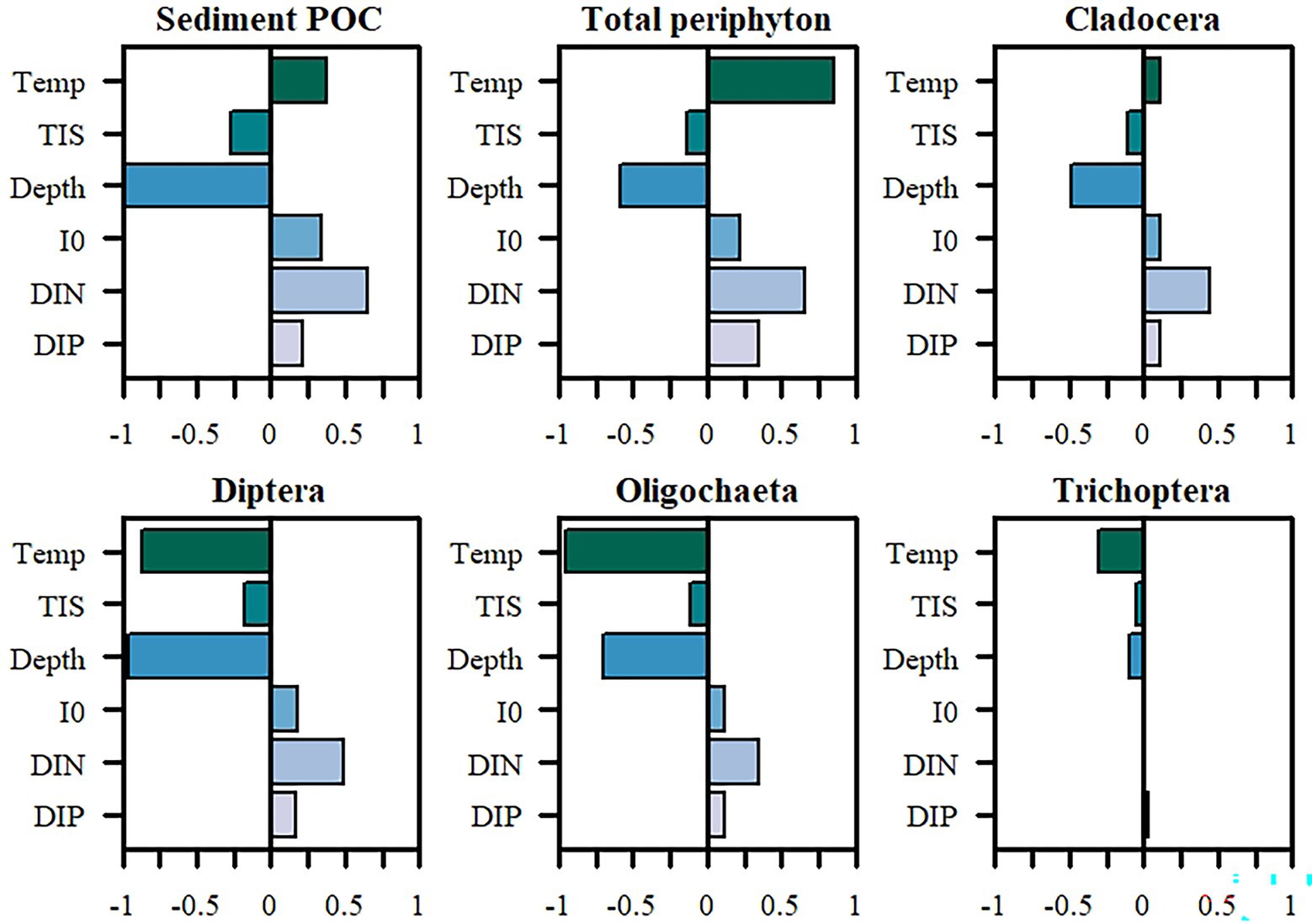
Figure 2. Partial rank correlation coefficients (PRCC) of the six tested factors and their impacts on biomass (g C/m2) of major prey items of the Topeka shiner. Temp, temperature; TIS, total inorganic solids; Depth, oxbow lake depth; I0, light intensity at water surface; DIN, total inorganic nitrogen; DIP, total inorganic phosphorus.
Temperature and depth had the largest positive effect on Topeka shiner adult and total biomass (Figure 3). Turbidity also correlated positively with Topeka shiner biomass, but to a much smaller extent than depth or temperature. Both nutrients and light intensity correlated negatively with Topeka shiner total population biomass. For the other fish species in the community, depth had the largest impact and correlated positively with sand shiner biomass and negatively with orange-spotted sunfish, and fathead minnow (Figure 3). Temperature had a positive effect on all species, except the orange-spotted sunfish. Turbidity consistently correlated negatively with fish biomass. Both nutrients and light intensity positively correlated with fish biomass, to different extents. Nitrates had the largest positive impact of the three abiotic factors, especially on the fathead minnow, followed by the orange-spotted sunfish and sand shiner.
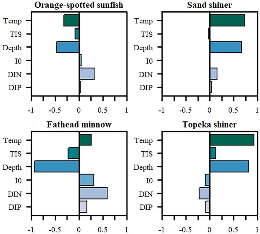
Figure 3. Partial rank correlation coefficients (PRCC) of the six tested factors and their impacts on the biomass (g C/m2) of the four fish species frequently co-occurring in oxbow habitats, including the Topeka shiner. Temp, temperature; TIS, total inorganic solids; Depth, oxbow lake depth; I0, light intensity at water surface; DIN, total inorganic nitrogen; DIP, total inorganic phosphorus.
Simulations where only single factors varied revealed that temperature had a positive effect on Topeka shiner biomass, but it affected its prey compartments differently (Figure 4). Cladocera, and to a smaller extent sediment POC (detritus) and periphyton showed a positive response to warming, whereas dipterans and oligochaetes showed a negative trend, and Trichoptera not showing any consistent trend.
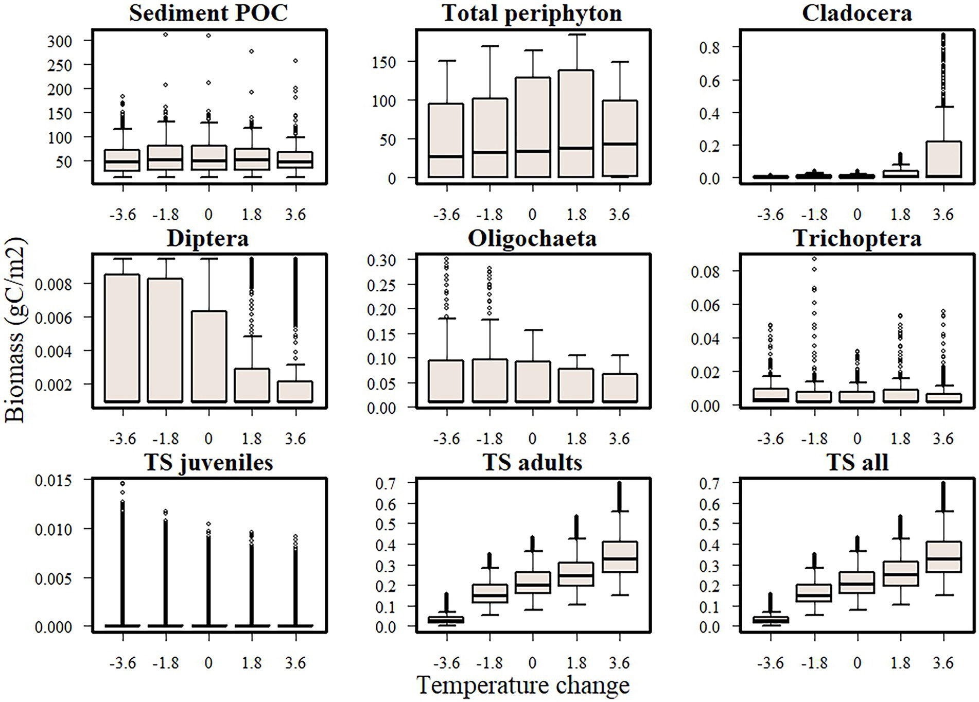
Figure 4. Boxplots of temperature effects on biomass of Topeka shiners (juveniles, adults, and the total population) and its main food items; in these single factor simulations, only temperature varied. Boxplots contain biomass values recorded over the last 20 years of simulations and across 10 simulated replicates. Boxes enclose the 25th and 75th percentile, the horizontal line denotes median values, the whiskers extend to the minimum and maximum value without outliers, and the dots show outliers.
Warmer temperatures resulted in an earlier onset of growth in Topeka shiner biomass (Figure 5A) and in an overall increased Topeka shiner biomass. There was not much difference in the onset between the two warmer conditions, but the biomass peak was 30% higher in the warmest temperature. The lowest tested temperature resulted in a delayed onset of biomass growth and in an overall lowest biomass when compared to any other environmental factor alteration. Depth had a less consistent impact on overall biomass (Figure 5B). The greatest depth (1.6 m) resulted in the largest overall biomass of Topeka shiner, but all other tested depths resulted in overall biomass similar to those under baseline conditions. Onset of biomass growth did not change across different depths tested. With regards to nutrients, only the lowest DIN amount (−1.2 mg/l) had a visible and substantial effect on Topeka shiner biomass (Figure 5C). Biomass resulting from all other alterations in nitrogen overlapped with the biomass simulated under baseline conditions.
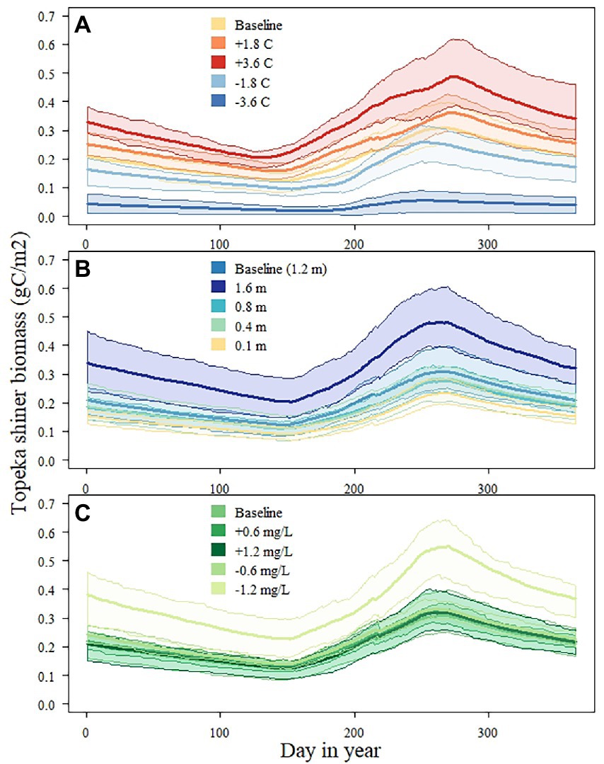
Figure 5. Topeka shiner biomass (total population) under different temperature (A), depth (B), and total dissolved nitrogen (DIN, C) conditions. Presented biomasses are averaged across the 10 simulated replicates; shaded areas represent the minimum and maximum value across the 10 replicates for each time point. Only 1 year (year 21) of the whole simulation period is shown for illustration.
As one of the main recovery strategies for listed species, habitat restoration aims at recreating the biotic and abiotic conditions that benefit population viability and persistence. Often, however, the optimal conditions for a species of interest are unknown. Field studies provide valuable data on species occurrence related to habitat and environmental quality parameters, but such studies are less amenable for systematic exploration of environmental parameter ranges and their combinations. Ecological modeling provides a platform facilitating comprehensive and systematic testing of those conditions and their ranges identified as potentially relevant for listed species. This simulation study identified water and habitat quality conditions that enhance the population biomass and persistence of the endangered Topeka shiner. Namely, nitrogen reduction, increasing temperature, and increasing depth had the largest positive impact on Topeka shiner biomass. These findings form a basis for additional empirical studies and for developing concrete management plans.
Overall, temperature changes had the most profound and consistent effect on Topeka shiner biomass, and to a lesser extent abundance (data not shown). Warming increased population biomass, whereas cooling reduced biomass to the extent that populations simulated the-3.6°C scenario maintained minimal biomass across the 40 simulated years. Warming can impact populations directly, by enhancing the physiological processes in individual fish, and indirectly, via effects on the food web. The effects on Topeka shiner were shown to be both direct and indirect, and the magnitude was largest when those were combined. Temperature directly affected the physiological rates of individual Topeka shiners, namely the consumption and respiration rates as defined in the Wisconsin fish model (Schmolke et al., 2019). Temperature is a major driver of organismal metabolism and increases rates until temperature equals the maximum value, after which organismal performance starts declining due to thermal stress (Huey and Stevenson, 1979). Temperatures simulated in the model were based on data gathered from Iowa stream stations and ranged between 3 and 26°C. Even with the maximum simulated increase of +3.6°C, the simulated temperatures rarely exceeded the optimal range (ranging between 27 and 34°C for consumption; Koehle, 2006; Koehle and Adelman, 2007). Increasing physiological rates thus sped up growth, maturation, and reproduction patterns, ultimately increasing Topeka shiner population growth. It is important to note that the information on the modeled thermal response was based on an experiment conducted with adult individuals (Koehle, 2006) and there is some uncertainty about the representativeness of these assumptions for egg and juvenile development. There is some indication that there is an ontogenetic change in thermal preferences, shown in Pacific salmon (Morita et al., 2010). However, until more life stage-specific information for Topeka shiner or similar species is available, the simplified assumption that thermal performance is consistent through ontogeny is valid. Furthermore, increased temperatures also resulted in earlier biomass growth of various prey items and ultimately allowed Topeka shiners to capitalize on earlier onsets of growth of their prey base. This extended time window with earlier biomass growth of preferred prey in addition to the increased metabolism in individual fish resulted in increased modeled population biomass of this endangered fish. Topeka shiner presence in natural habitats has been correlated with both warmer (Simpson et al., 2019) and cooler (Mammoliti, 2002) conditions. This species has also been found to have a higher thermal optimum than other species (Koehle, 2006; Koehle and Adelman, 2007), especially piscivorous fish, which would allow Topeka shiners to thrive in warmer areas. In this study, direct predation on Topeka shiner was not simulated, but a thermal refuge from predators could even further benefit Topeka shiner populations.
Depth correlated positively with Topeka shiner biomass, but the effect was less consistent than that of temperature. There was a clear increase in fish biomass only at the highest tested depth (at 1.6 m) whereas the Topeka shiner biomass overlapped in all other depth alterations. Depth correlated negatively with the preferred food items for simulated Topeka shiners, and for most of the co-occurring fish species, except for the sand shiner. Field surveys have found Topeka shiners preferred shallower off-channel habitats. Bakevich et al. (2013) reported an average depth of waterbodies of 0.54 m with Topeka shiners present (in contrast to and average depth of 0.63 m in waterbodies without the species). Other studies report water depths of off-channel habitats with Topeka shiner presence between 0.2 and 1.2 m (Dahle, 2001; Fischer et al., 2018). When oxbows are too shallow, they are at a higher chance of drying out and may cause local extirpations of Topeka shiner (Fischer et al., 2018). However, when oxbows are too deep, they may harbor more predators thus either causing local extinctions or reducing the Topeka shiner biomass (Mammoliti, 2002). Deeper oxbows, furthermore, have a greater capacity to buffer temperature fluctuations, and depth and temperature can often be correlated. In this simulation study, simplified assumptions about possible impacts of depth fluctuations were made: temperature was simulated as independent of the depths, oxbows did not dry out, and simulations did not include any predation on Topeka shiners, which means that the results were based on the increased availability of prey due to an increase in habitat (oxbow lake volume). In addition, the carrying capacity for Topeka shiner populations was increased because egg and larval survival was assumed to be reduced with increasing subadult and adult fish biomass in the whole simulated waterbody. Interestingly, the effect of depth alterations was unidirectional as there was no substantial decline in biomass when depth was reduced. Given that depth manipulation is one of the core activities of oxbow restoration efforts, a better understanding of how depth affects the biomass of this endangered fish is needed to better inform management and decision-making.
Nutrients, specifically dissolved inorganic nitrogen, were the third most impactful abiotic factors driving Topeka shiner biomass. Overall, DIN had a positive impact on most of Topeka shiner prey items, as well as on the biomass of co-occurring fish species, resulting in lower biomasses of most taxa with decreasing nitrogen. Interestingly, nitrogen reduction had a positive effect on the Topeka shiner biomass and abundance (results not shown), but this was only visible for the largest reduction tested (−1.2 mg/l). This could be a result of the shift in the diet reducing the proportion of detritus and periphyton with low energy density to more energy dense foods such as Trichoptera larvae which did not show a decline in biomass due to nitrogen reduction. A further exploration of the interaction between nitrogen reduction and the assumed feeding preferences on Topeka shiner population biomass is needed but was beyond the scope of this study. Importantly, the range of nutrient enrichment simulated in this study did not seem to have any effect on Topeka shiner biomass. There is very little to no information on the potential effects of nutrient enrichment on Topeka shiner population growth and persistence, but the effects of nutrient enrichment on aquatic ecosystems has been studied extensively (Scheffer et al., 1993; Smith et al., 1999). Nutrient enrichment can result in altered food webs (van der Lee et al., 2021), decreased species richness (Barker et al., 2008), in hypoxic and anoxic environments (Jenny et al., 2016), but there are also studies showing smaller impacts in aquatic communities (Feuchtmayr et al., 2009). The range of total dissolved nitrogen concentrations simulated in this study was based on concentrations measured in the Smeltzer oxbow in Iowa (Kalkhoff et al., 2016), but information on nitrogen concentrations and their effects on communities in oxbows is still largely absent.
In addition to providing habitat for listed and other species, oxbow lakes facilitate reductions of nitrate input from agricultural field to streams and rivers (Schilling et al., 2017, 2019). This nutrient reduction practice needs to be carefully balanced with the potential impact nutrient enrichment could have on listed and other species present in oxbow lakes. When it comes to direct toxicity of nitrogen, Topeka shiner have been shown to be less sensitive to ammonia, nitrites, and nitrates than the fathead minnow which is a species used in standard toxicity tests (Adelman et al., 2009). The US EPA’s recommendation of a maximum of 90 mg NO3/L is protective for Topeka shiner (Adelman et al., 2009), especially given that in multipurpose oxbow lakes the highest nitrate concentrations were 17 mg/l (Schilling et al., 2019) suggesting these are high quality habitats. In this study, direct toxicity of nitrates on any part of the ecosystem was not simulated; any positive or negative effect of nutrient enrichment was therefore mediated by the trophic interactions in the simulated oxbow lake. To ensure that the nutrient retention practice does not result in any adverse effects on the quality of these habitats for Topeka shiner populations, more targeted field and experimental studies should be conducted, as well as consistent long-term biomonitoring.
The full impact of potentially relevant environmental factors and their combinations on Topeka shiner population persistence needs further exploration. Field studies have shown mostly inconsistent correlations of Topeka shiner presence with temperature (Mammoliti, 2002; Simpson et al., 2019)¸ depth (Fischer et al., 2018) and water turbidity (Minckley and Cross, 1959; Kuitunen, 2001; Simpson et al., 2019), and negative correlation with the presence of woody vegetation (Simpson et al., 2019). To test all relevant factors and their combinations in the field would be logistically impossible, especially given the protected status of the endangered Topeka shiner. Applying ecological models to systematically explore impacts of single and multiple environmental factors offers opportunities to better understand and predict the presence and persistence of this and other listed species. Still, this modeling study does come with limitations. There were several potentially important factors that our models could not accommodate, for instance the influence of flooding frequency which has been suggested to be highly relevant for Topeka shiner presence in oxbow lakes (Fischer et al., 2018), implying the proximity to the stream and connectivity in the watershed play a major role in Topeka shiner colonization and occurrence. As such, stream proximity is one of the main factors determining new restoration efforts (Zambory et al., 2017), suggesting that a more in-depth exploration of the optimal spatial arrangement of oxbow restoration efforts would be beneficial and would likely require an application of a spatially explicit model, based on metapopulation theory (Hanski and Simberloff, 1997). Substrate type was another environmental characteristic that showed inconsistent impact on Topeka shiner presence (Kuitunen, 2001; Witte et al., 2009) that could not be tested in the model. Finally, given the scarcity of Topeka shiner population data, the model could not be validated with independent data which is the common challenge with listed species population models (Forbes et al., 2016; Schmolke et al., 2019). The hybrid model used in this study integrated the best available knowledge about this listed species, including its habitat and prey preferences, as well as other co-occurring species in the community. Its value is thus as a tool that can provide insight into relative impacts of tested environmental factors and their combinations on Topeka shiner population biomass.
This study identified three environmental factors that had the largest relative impact on Topeka shiner biomass. Based on these results, recommendations can be provided that could inform habitat restoration activities and support recovery plans for this listed species. Specifically, management of oxbows aiming at restoring long-term Topeka shiner could focus on establishing warmer water temperatures, for instance, by reducing the amount of shading by the riparian vegetation (Malcolm et al., 2008). There is some benefit of increased depth, but Topeka shiner populations persisted in shallower lakes too. Nutrient influx should be limited, but the exact magnitude of effects of nutrients is still unclear. For more explicit recommendations regarding impacts of the three factors, more exploration is needed. Ideally, the three identified factors would be further examined empirically under controlled conditions which would allow the testing and isolating effects of single and multiple factors. Semi-field study systems such as mesocosms (Stewart et al., 2013) could potentially be used to examine short-and long-term effects of these factors on Topeka shiner and its food web, though this could be challenging given the protected status of this endangered fish. Alternatively, more detailed measurements of relevant environmental factors in oxbows with and without Topeka shiner could provide further understanding of how these factors and their dynamics influence Topeka shiner population occurrence and persistence. Such studies should further be supported by ecological modeling, specifically to predict longer-term dynamics of oxbow lake communities under combinations of relevant environmental factors. Ecological, specifically population models have been recommended as risk assessment tools for listed species due to their integrative and predictive potential (NRC, 2013; Forbes et al., 2016). Such models have the capability of not only assessing the risk to populations of species of interest, but also to propose mitigation and management actions to ensure long-term population viability and persistence. This is especially relevant for species listed under the Endangered Species Act for which recovery plans are formulated containing recommendations about management strategies which should ultimately result in stable and persistent populations. Ecological models should increasingly support recovery plans to help identify factors that enhance species persistence and help design management practices that result in long-term population viability of listed species ultimately ensuring their timely delisting.
The datasets presented in this study can be found in online repositories. The names of the repository/repositories and accession number(s) can be found below: The input datasets and the model used in this study, including the relevant documentation, can be found in the GitHub repository (https://github.com/Waterborne-env/Topeka-shiner-model).
NG, AS, SB, and RB conceived and designed the study. CR and SB conducted the simulations. AS and CR analyzed the data. NG wrote the manuscript. All authors read and approved the manuscript.
Funding for this study was provided by Syngenta Crop Protection, LLC.
The authors acknowledge the input from Nicholas Green.
NG and RB were employed by the company Syngenta Crop Protection, LLC. AS and CR were employed by the company Waterborne Environmental Inc. SB was employed by the company Cardno, Inc.
Syngenta Crop Protection funded the study and employees of Waterborne Environmental and Cardno Inc are consulting companies commissioned to conduct the study.
All claims expressed in this article are solely those of the authors and do not necessarily represent those of their affiliated organizations, or those of the publisher, the editors and the reviewers. Any product that may be evaluated in this article, or claim that may be made by its manufacturer, is not guaranteed or endorsed by the publisher.
The Supplementary material for this article can be found online at: https://www.frontiersin.org/articles/10.3389/fevo.2022.1075244/full#supplementary-material
Adelman, I. R., Kusilek, L. I., Koehle, J., and Hess, J. (2009). Acute and chronic toxicity of ammonia, nitrite, and nitrate to the endangered Topeka shiner (Notropis topeka) and fathead minnows (Pimephales promelas). Environ. Toxicol. Chem. 28, 2216–2223. doi: 10.1897/08-619.1
Bakevich, B. D. (2012). Status, distribution, and habitat associations of Topeka shiners in west-Central Iowa. Ames: Iowa State University.
Bakevich, B. D., Pierce, C. L., and Quist, M. C. (2013). Habitat, fish species, and fish assemblage associations of the Topeka shiner in west-Central Iowa. N. Am. J. Fish Manag. 33, 1258–1268. doi: 10.1080/02755947.2013.839969
Barker, T., Hatton, K., O'Connor, M., Connor, L., and Moss, B. (2008). Effects of nitrate load on submerged plant biomass and species richness: results of a mesocosm experiment. Fundam. Appl. Limnol. 173, 89–100. doi: 10.1127/1863-9135/2008/0173-0089
Bartell, S. M., Brain, R. A., Hendley, P., and Nair, S. K. (2013). Modeling the potential effects of atrazine on aquatic communities in midwestern streams. Environ. Toxicol. Chem. 32, 2402–2411. doi: 10.1002/etc.2332
Bartell, S. M., Nair, S. K., Galic, N., and Brain, R. A. (2020). The comprehensive aquatic systems model (CASM): advancing computational capability for ecosystem simulation. Environ. Toxicol. Chem. 39, 2298–2303. doi: 10.1002/etc.4843
Bartell, S. M., Schmolke, A., Green, N., Roy, C., Galic, N., Perkins, D., et al. (2019). A hybrid individual-based and food web–ecosystem modeling approach for assessing ecological risks to the Topeka shiner (Notropis topeka): a case study with atrazine. Environ. Toxicol. Chem. 38, 2243–2258. doi: 10.1002/etc.4522
Bayless, M. A., McManus, M. G., and Fairchild, J. F. (2003). Geomorphic, water quality and fish community patterns associated with the distribution of Notropis topeka in a Central Missouri watershed. Am. Midl. Nat. 150, 58–72. doi: 10.1674/0003-0031(2003)150[0058:GWQAFC]2.0.CO;2
Blower, S. M., and Dowlatabadi, H. (1994). Sensitivity and uncertainty analysis of complex models of disease transmission: an HIV model, as an example. Int. Stat. Rev. 62, 229–243. doi: 10.2307/1403510
Brooks, T. M., Mittermeier, R. A., Mittermeier, C. G., Da Fonseca, G. A., Rylands, A. B., Konstant, W. R., et al. (2002). Habitat loss and extinction in the hotspots of biodiversity. Conserv. Biol. 16, 909–923. doi: 10.1046/j.1523-1739.2002.00530.x
Bybel, A., Simpson, N., Zambory, C., Pierce, C. L., Roe, K., and Weber, M. (2019). Boone River watershed stream fish and habitat monitoring, IA. Report to Fishers and Farmers Partnership. Ames, IA: Iowa State University.
Campbell, S. W., Szuwalski, C. S., Tabor, V. M., and deNoyelles, F. (2016). Challenges to reintroduction of a captive population of Topeka shiner (Notropis topeka) into former habitats in Kansas. Trans. Kans. Acad. Sci. 119, 83–92. doi: 10.1660/062.119.0112
Carnell, R. (2012). Lhs: Latin hypercube samples. R package, version 0.10. Available at: http://CRAN.R-project.org/package=lhs
Ceas, P., and Larson, K. (2010). "Topeka Shiner Monitoring in Minnesota: Year Seven ". (St. Paul: Minnesota Department of Natural Resources).
Dahle, S. P. (2001). Studies of Topeka Shiner (Notropis topeka) Life History and Distribution in Minnesota. St. Paul: University of Minnesota.
Deslauriers, D., Chipps, S. R., Breck, J. E., Rice, J. A., and Madenjian, C. P. (2017). Fish bioenergetics 4.0: an R-based modeling application. Fisheries 42, 586–596. doi: 10.1080/03632415.2017.1377558
Dubrovsky, N. M., Burow, K. R., Clark, G. M., Gronberg, J., Hamilton, P. A., Hitt, K. J., et al. (2010). The quality of our Nation’s waters—nutrients in the Nation’s streams and groundwater, 1992–2004. U. S. Geol. Surv. Circ. 1350:174.
Fahrig, L. (2003). Effects of habitat fragmentation on biodiversity. Annu. Rev. Ecol. Evol. Syst. 34, 487–515. doi: 10.1146/annurev.ecolsys.34.011802.132419
Feuchtmayr, H., Moran, R., Hatton, K., Connor, L., Heyes, T., Moss, B., et al. (2009). Global warming and eutrophication: effects on water chemistry and autotrophic communities in experimental hypertrophic shallow lake mesocosms. J. Appl. Ecol. 46, 713–723. doi: 10.1111/j.1365-2664.2009.01644.x
Fischer, J. R., Bakevich, B. D., Shea, C. P., Pierce, C. L., and Quist, M. C. (2018). Floods, drying, habitat connectivity, and fish occupancy dynamics in restored and unrestored oxbows of west Central Iowa, USA. Aquat. Conserv. Mar. Freshwat. Ecosyst. 28, 630–640. doi: 10.1002/aqc.2896
Forbes, V. E., Galic, N., Schmolke, A., Vavra, J., Pastorok, R., and Thorbek, P. (2016). Assessing the risks of pesticides to threatened and endangered species using population modeling: a critical review and recommendations for future work. Environ. Toxicol. Chem. 35, 1904–1913. doi: 10.1002/etc.3440
Gerken, J. E., and Paukert, C. P. (2013). Fish assemblage and habitat factors associated with the distribution of Topeka shiner (Notropis topeka) in Kansas streams. J. Freshw. Ecol. 28, 503–516. doi: 10.1080/02705060.2013.792754
Groom, M. J., Meffe, G. K., Carroll, C. R., and Andelman, S. J. (2006). Principles of Conservation Biology. Sunderland: Sinauer Associates.
Haines, B. J. (2017). Characterization of Hydrology and Water Quality at a Restored Oxbow: Ecosystem Services Achieved in Year One. Iowa: University of Iowa.
Hanski, I., and Simberloff, D. (1997). “The metapopulation approach, its history, conceptual domain, and application to conservation,” in Metapopulation Biology, Ecology, Genetics, and Evolution. eds. I. A. Hanski and M. E. Gilpin (New York: Academic Press), 5–26.
Hanson, P., Johnson, T., Schindler, D., and Kitchell, J. (1997). Fish Bioenergetics 3.0 Software for Windows®. Madison, WI: University of Wisconsin, Sea Grant Institute,.
Hatch, J. T., and Besaw, S. (2001). Food use in Minnesota populations of the Topeka shiner (Notropis topeka). J. Freshw. Ecol. 16, 229–233. doi: 10.1080/02705060.2001.9663807
Heinrichs, J. A., Aldridge, C. L., Gummer, D. L., Monroe, A. P., and Schumaker, N. H. (2018). Prioritizing actions for the recovery of endangered species: emergent insights from greater sage-grouse simulation modeling. Biol. Conserv. 218, 134–143. doi: 10.1016/j.biocon.2017.11.022
Huey, R. B., and Stevenson, R. D. (1979). Integrating thermal physiology and ecology of ectotherms: a discussion of approaches. Am. Zool. 19, 357–366. doi: 10.1093/icb/19.1.357
Jenny, J.-P., Francus, P., Normandeau, A., Lapointe, F., Perga, M.-E., Ojala, A., et al. (2016). Global spread of hypoxia in freshwater ecosystems during the last three centuries is caused by rising local human pressure. Glob. Chang. Biol. 22, 1481–1489. doi: 10.1111/gcb.13193
Jones, C. S., Kult, K., and Laubach, S. A. (2015). Restored oxbows reduce nutrient runoff and improve fish habitat. J. Soil Water Conserv. 70, 69A–72A. doi: 10.2489/jswc.70.3.69A
Kalkhoff, S. J., Hubbard, L. E., and Schubauer-Berigan, J. P. (2016). "The Effect of Restored and Native Oxbows on Hydraulic Loads of Nutrients and Stream Water Quality ". Cincinnati, OH: US Environmental Protection Agency.
Kerns, H. A., and Bonneau, J. L. (2002). Aspects of the life history and feeding habits of the Topeka shiner (Notropis topeka) in Kansas. Trans. Kans. Acad. Sci. 105, 125–142. doi: 10.1660/0022-8443(2002)105[0125:AOTLHA]2.0.CO;2
Kim, S. (2015). Ppcor: an R package for a fast calculation to semi-partial correlation coefficients. Commun. Stat. Appl. Methods 22, 665–674. doi: 10.5351/CSAM.2015.22.6.665
Koehle, J. J. (2006). The Effects of High Temperature, Low Dissolved Oxygen, and Asian Tapeworm Infection on Growth and Survival of the Topeka Shiner, Notropis topeka. Minneapolis, MN: University of Minnesota.
Koehle, J. J., and Adelman, I. R. (2007). The effects of temperature, dissolved oxygen, and Asian tapeworm infection on growth and survival of the Topeka shiner. Trans. Am. Fish. Soc. 136, 1607–1613. doi: 10.1577/T07-033.1
Kuitunen, A. (2001). "Microhabitat and Instream Flow Needs of the Topeka shiner in the Rock River Watershed, MN. Final Report. St. Paul: Minnesota Department of Natural Resources.
Malcolm, I. A., Soulsby, C., Hannah, D. M., Bacon, P. J., Youngson, A. F., and Tetzlaff, D. (2008). The influence of riparian woodland on stream temperatures: implications for the performance of juvenile salmonids. Hydrol. Process. 22, 968–979. doi: 10.1002/hyp.6996
Mammoliti, C. S. (2002). The effects of small watershed impoundments on native stream fishes: a focus on the Topeka shiner and Hornyhead chub. Trans. Kans. Acad. Sci. 105, 219–231. doi: 10.1660/0022-8443(2002)105[0219:TEOSWI]2.0.CO;2
McGowan, C. P., Catlin, D. H., Shaffer, T. L., Gratto-Trevor, C. L., and Aron, C. (2014). Establishing endangered species recovery criteria using predictive simulation modeling. Biol. Conserv. 177, 220–229. doi: 10.1016/j.biocon.2014.06.018
Minckley, W. L., and Cross, F. B. (1959). Distribution, habitat, and abundance of the Topeka shiner Notropis topeka (Gilbert) in Kansas. Am. Midl. Nat. 61, 210–217. doi: 10.2307/2422352
Morita, K., Fukuwaka, M.-A., Tanimata, N., and Yamamura, O. (2010). Size-dependent thermal preferences in a pelagic fish. Oikos 119, 1265–1272. doi: 10.1111/j.1600-0706.2009.18125.x
Nagle, B. (2014). Revisits to Known Topeka shiner Localities: Further Evidence of Decline in Minnesota. Saint Paul, MN: Minnesota Department of Natural Resources, Division of Ecological and Water Resources.
NRC (Ed.) (2013). Assessing risks to endangered and threatened species from pesticides. Committee on ecological risk assessment under FIFRA and ESA, board on environmental studies and toxicology, division on earth and life studies, National Research Council of the National Academies. Washington, DC: The National Academies Press.
Prentice, A. L. (2013). Land use in Topeka Shiner (Notropis topeka) watersheds in Missouri and efficacy of orangespotted sunfish (Lepomis humilis) as spawning associates.” PhD diss.
Scheffer, M., Hosper, S. H., Meijer, M. L., Moss, B., and Jeppesen, E. (1993). Alternative equilibria in shallow lakes. Trends Ecol. Evol. 8, 275–279. doi: 10.1016/0169-5347(93)90254-M
Schilling, K. E., Kult, K., Wilke, K., Streeter, M., and Vogelgesang, J. (2017). Nitrate reduction in a reconstructed floodplain oxbow fed by tile drainage. Ecol. Eng. 102, 98–107. doi: 10.1016/j.ecoleng.2017.02.006
Schilling, K. E., Wilke, K., Pierce, C. L., Kult, K., and Kenny, A. (2019). Multipurpose oxbows as a nitrate export reduction practice in the agricultural Midwest. Agric. Environ. Lett. 4:190035. doi: 10.2134/ael2019.09.0035
Schmolke, A., Bartell, S. M., Roy, C., Desmarteau, D., Moore, A., Cox, M. J., et al. (2021). Applying a hybrid modeling approach to evaluate potential pesticide effects and mitigation effectiveness for an endangered fish in simulated oxbow habitats. Environ. Toxicol. Chem. 40, 2615–2628. doi: 10.1002/etc.5144
Schmolke, A., Bartell, S. M., Roy, C., Green, N., Galic, N., and Brain, R. (2019). Species-specific population dynamics and their link to an aquatic food web: a hybrid modeling approach. Ecol. Model. 405, 1–14. doi: 10.1016/j.ecolmodel.2019.03.024
Schrank, S., Guy, C., Whiles, M., and Brock, B. (2001). Influence of instream and landscape-level factors on the distribution of Topeka shiners Notropis topeka in Kansas streams. Copeia 2001, 413–421. doi: 10.1643/0045-8511(2001)001[0413:IOIALL]2.0.CO;2
Schwartz, M. W. (2008). The performance of the endangered species act. Annu. Rev. Ecol. Evol. Syst. 39, 279–299. doi: 10.1146/annurev.ecolsys.39.110707.173538
Simpson, N. (2018). “Occurrence, abundance, and associations of Topeka Shiners and species of greatest conservation need in streams and oxbows of Iowa and Minnesota”. Graduate Theses and Dissertations 16466. https://lib.dr.iastate.edu/etd/16466
Simpson, N. T., Bybel, A. P., Weber, M. J., Pierce, C. L., and Roe, K. J. (2019). Occurrence, abundance and associations of Topeka shiners (Notropis topeka) in restored and unrestored oxbows in Iowa and Minnesota, USA. Aquat. Conserv. Mar. Freshwat. Ecosyst. 29, 1735–1748. doi: 10.1002/aqc.3186
Smith, V. H., Tilman, G. D., and Nekola, J. C. (1999). Eutrophication: impacts of excess nutrient inputs on freshwater, marine, and terrestrial ecosystems. Environ. Pollut. 100, 179–196. doi: 10.1016/S0269-7491(99)00091-3
Stark, W. J., Luginbill, J. S., and Eberle, M. E. (2002). Natural history of a relict population of Topeka shiner (Notropis topeka) in northwestern Kansas. Trans. Kans. Acad. Sci. 105, 143–152. doi: 10.1660/0022-8443(2002)105[0143:NHOARP]2.0.CO;2
Stewart, R. I. A., Dossena, M., Bohan, D. A., Jeppesen, E., Kordas, R. L., Ledger, M. E., et al. (2013). “Chapter two-Mesocosm experiments as a tool for ecological climate-change research,” in Advances in Ecological Research. eds. G. Woodward and E. J. O'Gorman (Cambridge, MA: Academic Press), 71–181.
Tabor, V. M. (1998). Endangered and threatened wildlife and plants; final rule to list the Topeka shiner as endangered. Fed. Reg. 63, 69008–69021.
U.S. Fish and Wildlife Service (2018). "Species Status Assessment Report for Topeka Shiner (Notropis topeka), Version 1.0. Denver, CO: U.S. Fish and Wildlife Service, Region 6.
U.S. Fish and Wildlife Service (2019). "Recovery Plan for the Topeka Shiner (Notropis topeka). Draft.". (Manhattan, KS: U.S. Fish and Wildlife Service, Mountain-Prairie Region).
van der Lee, G. H., Vonk, J. A., Verdonschot, R. C., Kraak, M. H., Verdonschot, P. F., and Huisman, J. (2021). Eutrophication induces shifts in the trophic position of invertebrates in aquatic food webs. Ecology 102:e03275. doi: 10.1002/ecy.3275
Wall, S. S., Berry, J., Charles, R., Blausey, C. M., Jenks, J. A., and Kopplin, C. J. (2004). Fish-habitat modeling for gap analysis to conserve the endangered Topeka shiner (Notropis topeka). Can. J. Fish. Aquat. Sci. 61, 954–973. doi: 10.1139/f04-017
Werblow, S. (2019). Oxbows: conservation treasures. The Progressive Farmer. https://www.dtnpf.com/agriculture/web/ag/news/article/2019/01/01/old-river-bends-offer-rich-reward
Winston, M. R. (2002). Spatial and temporal species associations with the Topeka shiner (Notropis topeka) in Missouri. J. Freshw. Ecol. 17, 249–261. doi: 10.1080/02705060.2002.9663893
Witte, C., Wildhaber, M., Arab, A., and Noltie, D. B. (2009). Substrate choice of territorial male Topeka shiners (Notropis topeka) in the absence of sunfish (Lepomis sp.). Ecol. Freshw. Fish 18, 350–359. doi: 10.1111/j.1600-0633.2008.00351.x
Keywords: individual-based model, aquatic ecosystem model, endangered species act, habitat restoration, water temperature, oxbow depth, dissolved organic nitrogen
Citation: Galic N, Schmolke A, Bartell S, Roy C and Brain R (2023) Applying a hybrid model to support management of the endangered Topeka shiner in oxbow habitats. Front. Ecol. Evol. 10:1075244. doi: 10.3389/fevo.2022.1075244
Edited by:
Jesús N. Pinto-Ledezma, University of Minnesota, United StatesReviewed by:
Kelly Da Silva E. Souza, Institutos Nacionais de Ciência e Tecnologia (INCT), BrazilCopyright © 2023 Galic, Schmolke, Bartell, Roy and Brain. This is an open-access article distributed under the terms of the Creative Commons Attribution License (CC BY). The use, distribution or reproduction in other forums is permitted, provided the original author(s) and the copyright owner(s) are credited and that the original publication in this journal is cited, in accordance with accepted academic practice. No use, distribution or reproduction is permitted which does not comply with these terms.
*Correspondence: Nika Galic, ✉ bmlrYS5nYWxpY0BzeW5nZW50YS5jb20=
Disclaimer: All claims expressed in this article are solely those of the authors and do not necessarily represent those of their affiliated organizations, or those of the publisher, the editors and the reviewers. Any product that may be evaluated in this article or claim that may be made by its manufacturer is not guaranteed or endorsed by the publisher.
Research integrity at Frontiers
Learn more about the work of our research integrity team to safeguard the quality of each article we publish.