Historical reconstruction of aquatic vegetation of typical lakes in Northeast China based on an improved CA-Markov model

Aquatic vegetation is an important marker of the change in the lake ecosystem. It plays an important supporting role in the lake ecosystem, and its abundance and cover changes affect the ecosystem balance. Collecting accurate long-term distribution data on aquatic vegetation can help monitor the change in the lake ecosystem, thereby providing scientific support for efforts to maintain the balance of the ecosystem. This work aimed to establish an improved CA-Markov model to reconstruct historical potential distribution of aquatic vegetation in the two typical lakes (Xingkai Lake and Hulun Lake) in Northeast China during 1950s to 1960s. We firstly analyzed remote sensing data on the spatial distribution of aquatic vegetation data in two lakes in six periods from the 1970 to 2015. Then, we built a transfer probability matrix for changes in hydrothermal conditions (temperature and precipitation) based on similar periods, and we designed suitability images using the spatial frequency and temporal continuity of the constraints. Finally, we established an improved CA-Markov model based on the transfer probability matrix and suitability images to reconstruct the potential distributions of aquatic vegetation in the two northeastern lakes during the 1950s and 1960s. The results showed the areas of aquatic vegetation in the 1950s and 1960s were 102.37 km² and 100.7 km² for Xingkai Lake and 90.81 km² and 88.15 km² for Hulun Lake, respectively. Compared with the traditional CA-Markov model, the overall accuracy of the improved model increased by more than 50%, which proved the improved CA-Markov model can be used to effectively reconstruct the historical potential distribution of aquatic vegetation. This study provides an accurate methodology for simulating the potential historical distributions of aquatic vegetation to enrich the study of the historical evolution of lake ecosystem.

Introduction

Lakes are an important foundation for economic development and ecological security in China. Northern Lakes account for 37% of the total lake area in China, providing significant strategic support services for ensuring the socioeconomic development and ecological security of China (Bu et al., 2013; Wang et al., 2015; Dai et al., 2021). Aquatic vegetation—including submerged vegetation, floating leaf vegetation, and emergent vegetation—can clarify water, decrease the rate of nutrient cycling, suppress waves, improve water quality, and provide food and habitats for many aquatic animals (Jeppesen et al., 1998; Horppila and Nurminen, 2003; Orth et al., 2006). Aquatic plants are also important regulators of the evolution and balance of the lake ecosystem, and they play an important role in maintaining lake ecosystems and waterfowl and phytoplankton communities (Roijackers et al., 2004; Bilton et al., 2006).

Since the 1950s, numerous studies have demonstrated that lake ecosystems have undergone a severe decline due to the combined effects of climate change and human activities (Sand-Jensen et al., 2000; Moss et al., 2011). Similarly, there has been a significant decline in aquatic vegetation of lakes; this has further exacerbated the loss of ecosystem services, resulting in severe ecological problems for lake ecosystems. Therefore, quantifying the historical distributions of aquatic vegetation—including its abundance and dynamics—not only helps reveal the response of lake ecosystems to climate change but also supports the conservation of lake biodiversity (Körner and Nicklisch, 2002; Liira et al., 2010; Kolada et al., 2014; Qing et al., 2020).

At present, there are two main ways to obtain information on the historical spatial distribution of aquatic vegetation in lakes. (1) Historical field survey records: Field surveys and monitoring of aquatic vegetation provide important original information on the distribution of aquatic vegetation, according to the literature. However, studies of the distribution, abundance, and dynamics of aquatic vegetation in lakes have focused on a few lakes in a small geographical area (Sand-Jensen et al., 2000; Körner and Nicklisch, 2002) and have covered a short historical period of field surveying data, mostly after the 1980s. In addition, most field surveys have recorded distributions in the form of points, rather than continuous spatial data, limiting the application of aquatic vegetation data in the geospatial model. (2) Historical remote sensing image interpretation: Remote sensing technologies have become the most effective methods for identifying and monitoring the historical spatial patterns of aquatic vegetation due to their ability to support large-scale, abundant, long-term observation based on spectral indices (Fornes et al., 2006; Laba et al., 2010; Luo et al., 2017; Song et al., 2019). Nevertheless, the earliest satellite image data date back to the 1970s (i.e., Landsat MSS satellite data), making it impossible to obtain information on the spatial distribution of aquatic vegetation in lakes before the 1970s. Considering the low levels of disturbance in the lakes caused by human activities during the 1950s and 1960s, aquatic vegetation was mainly affected by climate change. Therefore, the spatial distribution and dynamics of aquatic vegetation can be used to predict the response of aquatic vegetation to natural environmental change. However, no datasets on the distribution and changes in aquatic vegetation were obtained using the aforementioned methods during the 1950s and 1960s, which hinders a comprehensive and systematic assessment of aquatic vegetation for lakes.

The CA-Markov model, which incorporates the theories of Markov chain and cellular automata (Sang et al., 2011), is widely used to simulate the land surface type (Zhou et al., 2020; Fu et al., 2022). In addition to predicting temporal and spatial patterns of future changes in the land surface type, it also reconstructs historical land surface characteristics (Mondal et al., 2016; He et al., 2022). However, as changes in the land surface type are often affected by many factors, the common CA-Markov model cannot always accurately simulate historical surface type changes. In recent research, the integration of spatial information and decision conditions used in multi-criteria evaluations has demonstrated a powerful capability to control the comprehensive effects of many factors. The essence of this technique lies in the production of suitability images of land surface type to improve the predictive ability of the CA-Markov model (Getachew et al., 2021). The collection of suitability images is scored by each influential factor, producing constraint conditions for the CA model (Ahmed, 2011). The factors used in the suitability images cover sociometric elements and environmental dimensions, and the images translate this information into manageable information or measurable parameters. The selection of factors is usually based on ranking results from the analytic hierarchy process (AHP) and principle component analysis (Lee and Chan, 2008), as well as scores assigned based on experience and literature reviews (Zavadskas and Antucheviciene, 2007). However, previous studies have faced a serious problem: the factor selection and suitability score assignment were unrelated to the land surface change for the given model. Therefore, establishing appropriate suitability images to improve the CA-Markov model is crucial for the high-accuracy historical reconstruction of land surface features.

As the land surface system has the same land cover (Yang et al., 2019), aquatic vegetation and the water body can be deemed two lake cover types in the lake ecosystem. In this study, we developed a novel calculation method for the previous transfer probability matrix based on the similarity of change in annual average temperature and the annual precipitation of different periods. Also, we developed a new collection of suitability images based on the constraints of the spatial frequency of occurrence and the temporal recency effect in the simulation process to improve the accuracy of the CA-Markov model. Then, by combining the transfer probability matrix and suitability images, we built an improved CA-Markov model to reconstruct the historical distribution of aquatic vegetation in Xingkai Lake and Hulun Lake during the 1950s and 1960s. We evaluated the model accuracy by comparing the results of the common CA-Markov model simulation and the remote sensing interpretation; the model simulation error rate (MSER) was used to evaluate model improvement. The research results provide scientific data for lake ecosystem research and lake responses to climate change while enriching the method of simulating and reconstructing aquatic vegetation in historical periods.

Materials and methods

Study area

Xingkai Lake and Hulun Lake, located in Northeast China, were selected to reconstruct the historical potential distribution of aquatic vegetation using the improved CA-Markov model (Figure 1) and are located in a temperate humid and a semi-humid monsoon climate zone, respectively. Precipitation is mainly concentrated in summer and autumn, with abundant water in the lakes during the information period, followed by a long freezing period in winter, with a low water level in the lakes. According to the literature, aquatic vegetation is rich in both lakes and has undergone dramatic changes in the past decades (Yuan et al., 2018; Mao et al., 2022).

FIGURE 1

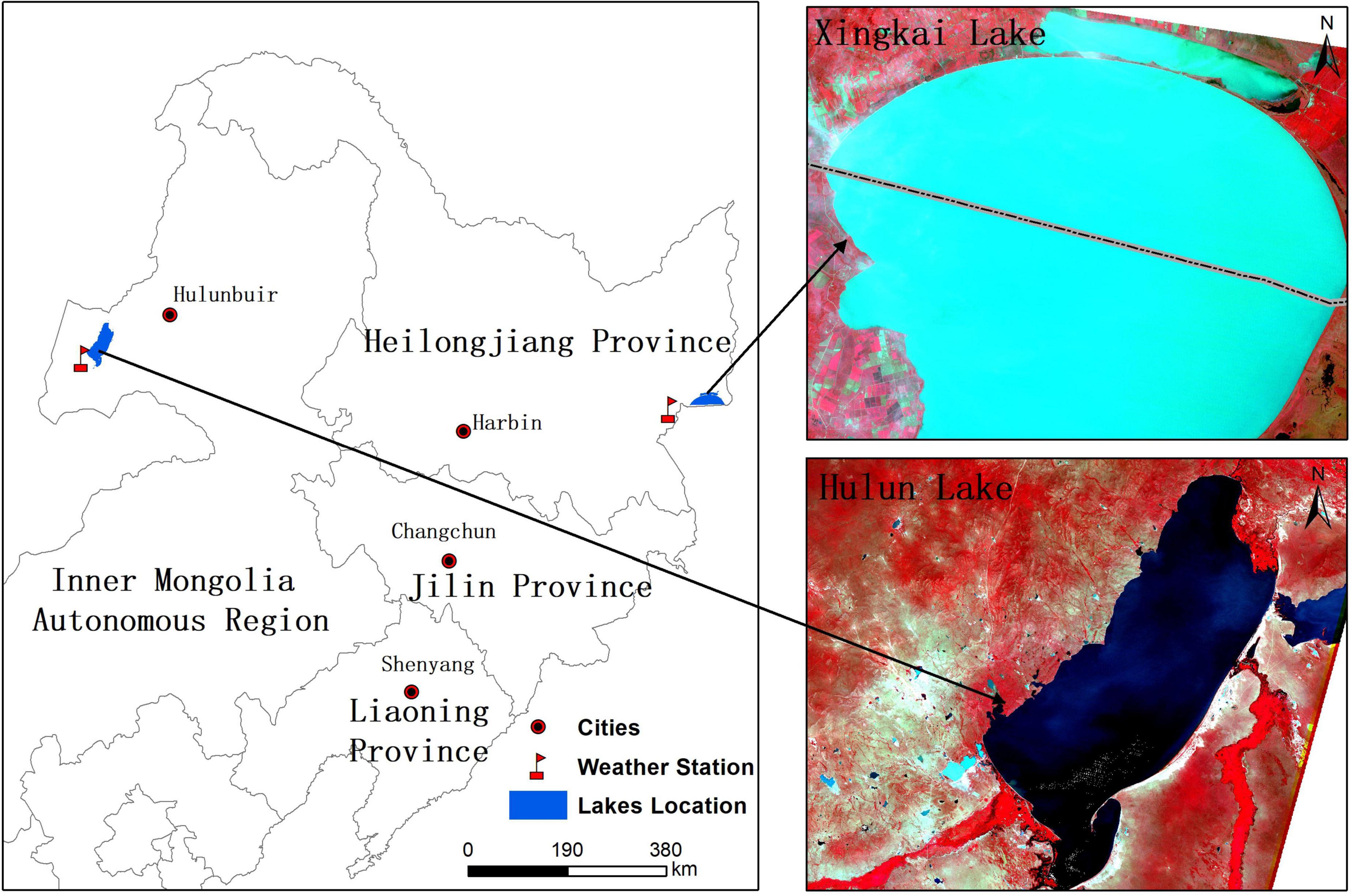
Figure 1. Location of lakes in the study area of Northeast China.

Xingkai Lake is the largest freshwater lake in northeastern Asia. It is located on the border between China and Russia, with the geographical coordinates of 131°58’30”∼133°07’30 “E and 45°01’00”∼45°34’30 “N. Xingkai Lake is divided into big Xingkai Lake and small Xingkai Lake by Chinese people, with a total surface area of 4,190 km², an average water depth of 4.5 m, and a maximum depth of 10 m. The aquatic vegetation is mainly concentrated in small Xingkai Lake.

Hulun Lake is located in the western part of the Hulunbuir grassland, with geographical coordinates of 117°00’10”∼117°41’40 “E and 48°30’40”∼49°20’40 “N and a total area of 2,339 km². A total of four rivers empty into Hulun Lake, including the Kherlen, Hailar, Halaha, and Orxon rivers. The aquatic vegetation is concentrated in the estuary.

Because of the different sources of lake water replenishment, the two lakes exhibit different levels of variability in water storage. In addition, both the lakes are located in a mid-latitude region, where the lake ecosystems are sensitive to global climate change, and both lakes have experienced minimal human disturbance during the 1950s and 1960s. Therefore, the lakes are excellent research areas for exploring the historical distribution and changes in aquatic vegetation in relation to the response of lake ecosystems to climate change.

Data and processing

Landsat images of the two lakes during the 1970–2015 (1970s, 1980s, 1990s, 2000, 2010, and 2015) were downloaded from the Geospatial Data Cloud¹. The images were processed by radiometric and geometric calibration (Table 1). Then, three indices (NDVI, SAVI, and NDWI), whose thresholds were determined by the Otsu algorithm, were calculated to gain 200 training samples of aquatic vegetation for each lake based on the decision tree model. A random forest model was adopted to obtain the distribution of aquatic vegetation using 150 training samples for each lake from imagery for the six periods. The remaining 50 samples were used to verify the model, and the total accuracy was over 85%.

TABLE 1

Table 1. Timelines, path, and row of Landsat imagery data.

The datasets acquired from the remote sensing imagery served as the basis for the reconstruction of the historical spatial distribution of aquatic vegetation in the 1950s and 1960s. Given the demarcation of the lake extent for reconstruction by the CA-Markov model, we downloaded Zhang Guoqing’s 1960–2015 lake boundary datasets in China (Zhang et al., 2019) to restrict the extent of the simulation of aquatic vegetation. In order to analyze climatic changes in different historical periods, we downloaded meteorological datasets on the nearest meteorological stations of the two lakes from the National Meteorological Center². Then, the annual average temperature and annual precipitation were calculated from the 1950 to 2021.

Methods

The CA-Markov model combines the ability of the CA model to simulate complex spatial changes with the advantages of the Markov model for temporal prediction (Yang et al., 2016, 2019). By adding continuous spatial distribution elements to Markov chains and using multiple constraints and limiting factors, the model can achieve spatial predictions for future features and accurately reconstruct historical states. This allows for the high-accuracy simulation of ecosystem changes.

The Markov chain model is a quantitative description of transfer states using the area transfer matrix and the area probability transfer matrix between the feature states in different periods. Its mathematical equation is as follows:

$S_{ij}=\left[\begin{array}{ccc}\hfill \begin{array}{cc}\hfill s_{11}{s}_{12}\hfill & \\ \hfill s_{21}{s}_{22}\hfill & \end{array}\mathrm{\cdots }\begin{array}{c}\hfill s_{1n}\hfill \\ \hfill s_{2n}\hfill \end{array}\hfill & & \\ \hfill \mathrm{⋮}\mathrm{\ddots }\mathrm{⋮}\hfill & & \\ \hfill \begin{array}{cc}\hfill s_{n1}{s}_{n2}\hfill & \end{array}\mathrm{\cdots }{s}_{nn}\hfill & & \end{array}\right]$

$P_{ij}=\left[\begin{array}{ccc}\hfill \begin{array}{cc}\hfill p_{11}{p}_{12}\hfill & \\ \hfill p_{21}{p}_{22}\hfill & \end{array}\mathrm{\cdots }\begin{array}{c}\hfill p_{1n}\hfill \\ \hfill p_{2n}\hfill \end{array}\hfill & & \\ \hfill \mathrm{⋮}\mathrm{\ddots }\mathrm{⋮}\hfill & & \\ \hfill \begin{array}{cc}\hfill p_{n1}{p}_{n2}\hfill & \end{array}\mathrm{\cdots }{p}_{nn}\hfill & & \end{array}\right]$

where i, j = 1,2,…,n represent the land-use types before and after transfer, S_ij is the land-use area transfer matrix, and P_ij is the land-use area transfer probability matrix.

The cellular automata (CA) model is a discontinuous spatiotemporal dynamics model characterized by discrete time, space, and state (Fu et al., 2018). Each cell in the CA system has discrete states, and each raster cell corresponds to a cell whose transformation rules are localized in time and space. These local rules interact to form a dynamic evolutionary system expressed by the following mathematical formula:

$S_{t+1}=f(S_t,N)$

where S_(t+1) is the state of the tuple at the previous moment, S_t is the state of the tuple at the current moment, N is the tuple domain, and f is the local space tuple transfer rule.

The implementation of the CA-Markov model requires two important parameters: the transition probability matrix and suitability images. The transition probability matrix can be used to describe the transition probability of the land surface type transformation for two time intervals. The matrix is used to predict and simulate the land surface type transition areas for both future and historical periods. The suitability images are based on multiple criteria (transformation rules) that determine the state of the feature at the next moment. The prediction of spatial features is achieved computationally by adding continuous, spatially distributed features to the Markov chain using multiple constraints and limiting factors.

Transfer probability matrix module

The transfer probability matrix is derived from the Markov chain and determines the transformation rule from the start status to the end status for the land surface types; it contains joint probabilities, which are the product of amplitude of the two states (Eberly and Carlin, 2000). It can also be considered as the transition rule for the CA model, which decides the cell number or probability of transformations between land surface types during the two periods. For the lakes, the distribution of the lake surface types (aquatic vegetation and water bodies) in the two time intervals can generate the transfer matrix of Markov probability. Considering the spatiotemporal correlation of the evolution of aquatic vegetation, more complex relationships between the changing pattern of aquatic vegetation and regional conditions were found. Moreover, the local climatic conditions directly affect the distribution and transformation probability of aquatic vegetation in the lake. Some research has shown that changes in aquatic vegetation are closely related to climate (Zhao et al., 2021), that is to say, if the change in climate conditions was similar for two periods, the transformation probability of aquatic vegetation is likely to be similar as well. For instance, assuming that the climate change scenario for 1960–1970 is similar to that for 1990–2000, we assigned similar transfer probability matrices for the two periods. Therefore, in this study, the changes in the annual average temperature and annual precipitation are selected as environmental factors to assist the Markov model for calculating the probability transfer matrix.

The dynamic evolution of aquatic vegetation is considered a transfer process. However, for the historical distribution of aquatic vegetation, reconstruction of the “possible states” was a reverse process in which past states are simulated from more recent states. To avoid the transferability of errors, we selected the aquatic vegetation in the 1970s as a baseline to simulate vegetation distribution in the 1950s and 1960s. Consequently, we used a 20-year step to simulate the spatial distribution of aquatic vegetation in lakes in the 1950s and a 10-year step to simulate the distribution in the 1960s.

Suitability image module

The probabilistic CA-Markov model is a potent simulator for predicting changes in the land surface type compared with other types of linear extrapolation models (Aaviksoo, 1993). The suitability images are based on multiple criteria (transformation rules) to determine the state of a cell at the next moment. The prediction of geomorphic elements is achieved scientifically by adding continuous, spatially distributed elements to the Markov chain using multiple limiting constraints. By incorporating the suitability images into the CA transformation rules and constraining the CA to change by itself, the defects of the cellular automata can be remedied and the simulation results can better reflect the complexity of the spatiotemporal evolution of land surface patterns.

Given the spatiotemporal succession of vegetation growth (Wang et al., 2020), the spatial occurrence frequency and temporal recency effect of aquatic vegetation growth in the historical period were selected as the two most important constraint factors to generate the suitability images. These images were then used to reconstruct the potential distribution zones of aquatic vegetation in this study. Based on the aquatic vegetation dataset obtained from remote sensing data for six periods from 1970 to 2015, the potential distribution zones of aquatic vegetation in the 1950s and 1960s were simulated at the pixel scale using the restrictive conditions of the two suitability images. Table 2 shows the definition of the relationship between the influencing factors and aquatic vegetation for the construction of the suitability images.

TABLE 2

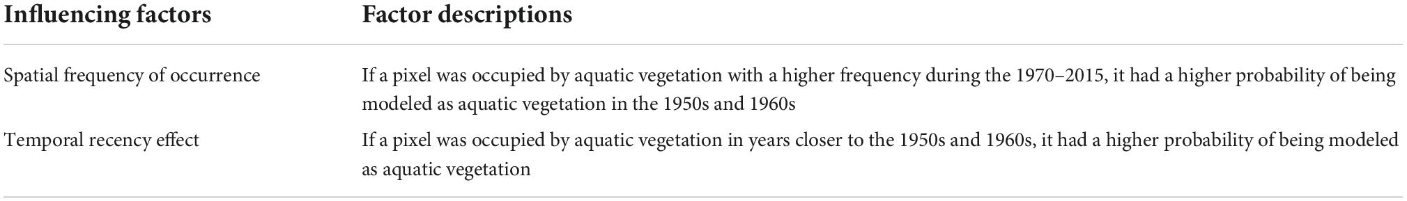
Table 2. Impact factors of the suitability images.

Spatial frequency of occurrence

Without considering the influence of temporal succession on the simulation, we defined the pixel as the basic unit for aquatic vegetation simulation. The probability of emergence for the aquatic vegetation during the 1950s and 1960s was controlled by the spatial frequency of occurrence in the six periods (1970–2015) for each pixel. Figure 2 shows the spatial occurrence frequency weighting analysis of aquatic vegetation. Pixels assigned a value of 1 represent aquatic vegetation, while pixels assigned a value of 0 represent a waterbody. The occurrence frequency of aquatic vegetation in the historical distribution data was superimposed to generate a judgment matrix. If the pixel value was larger in the judgment matrix, it was more likely to be simulated as aquatic vegetation. Finally, a spatial frequency weighting map of aquatic vegetation was generated (Figure 2).

FIGURE 2

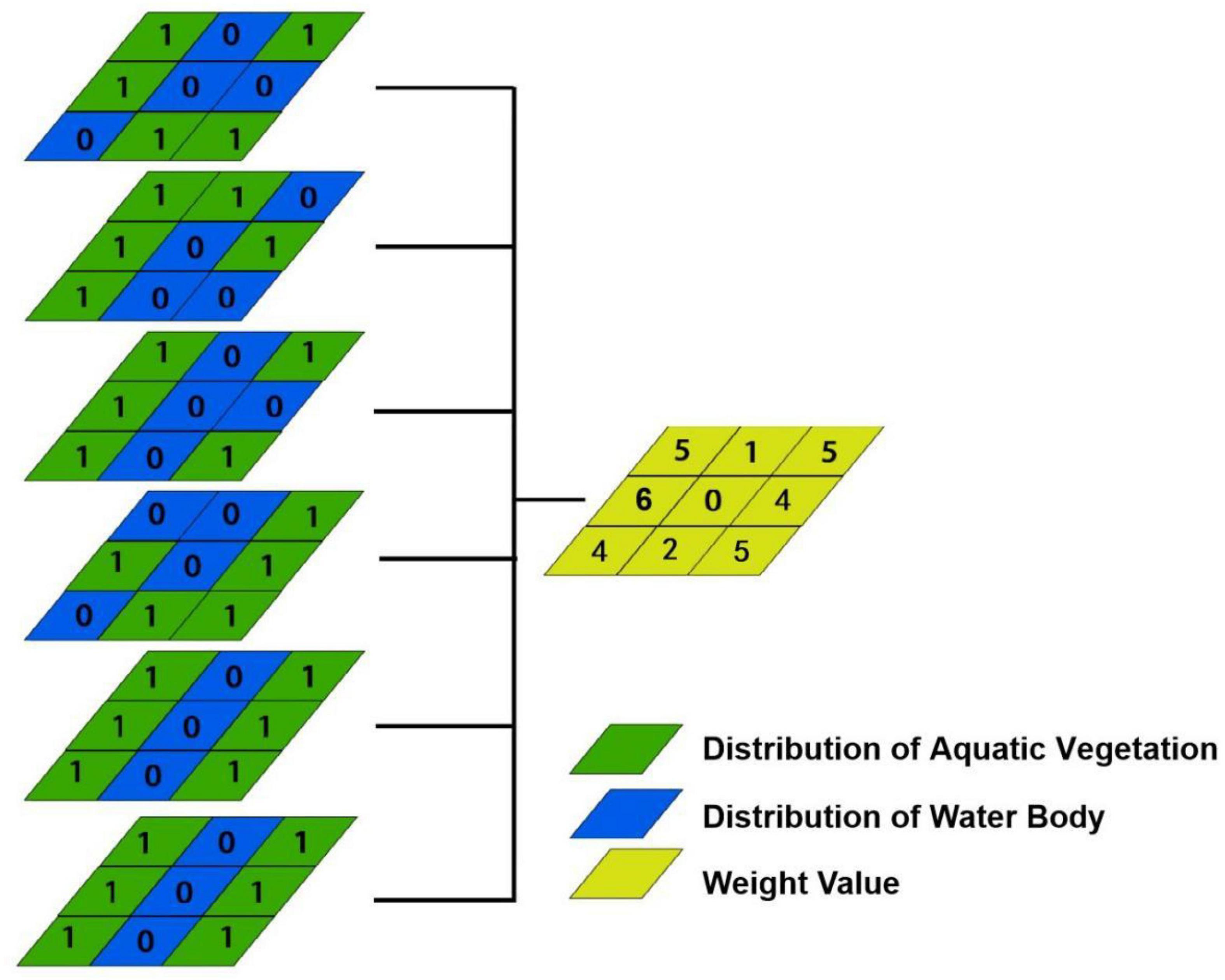
Figure 2. Spatial occurrence frequency weighting analysis map of aquatic vegetation.

Temporal recency effect

Given the influence of temporal succession on aquatic vegetation, there is a temporal recency effect for the simulation of aquatic vegetation. Periods closer to the simulated period were allocated a greater weight value. In this study, in the case of simulating the spatial distribution of aquatic vegetation in the 1960s, the image of 2015 was defined as the base weight, with a value of 1. The weight value increased by 1 every decade as the data approached the simulation periods. As a result, we constructed a linearly increasing weight matrix, where 2010 had a weight of 2, 2000 had a weight of 3, 1990 had a weight of 4, 1980 had a weight of 5, and 1970 had a weight of 6. If aquatic vegetation existed in multiple periods for the simulation target image pixel, the weight value was the sum of the weights of all the periods. For instance, if the input simulation pixel was aquatic vegetation in both the 1970s and 1980s, the weight was 11: the sum of weight 5 in the 1980s and weight 6 in the 1970s. Based on the temporal recency effect, pixels of the different periods were assigned differentiated weights calculated by overlay analysis. As a result, 15 different weight assignments occurred in the prediction distribution of aquatic vegetation in the 1960s. Figure 3 shows a temporal recency effect weighting analysis map of aquatic vegetation, including the results of the weight assignments.

FIGURE 3

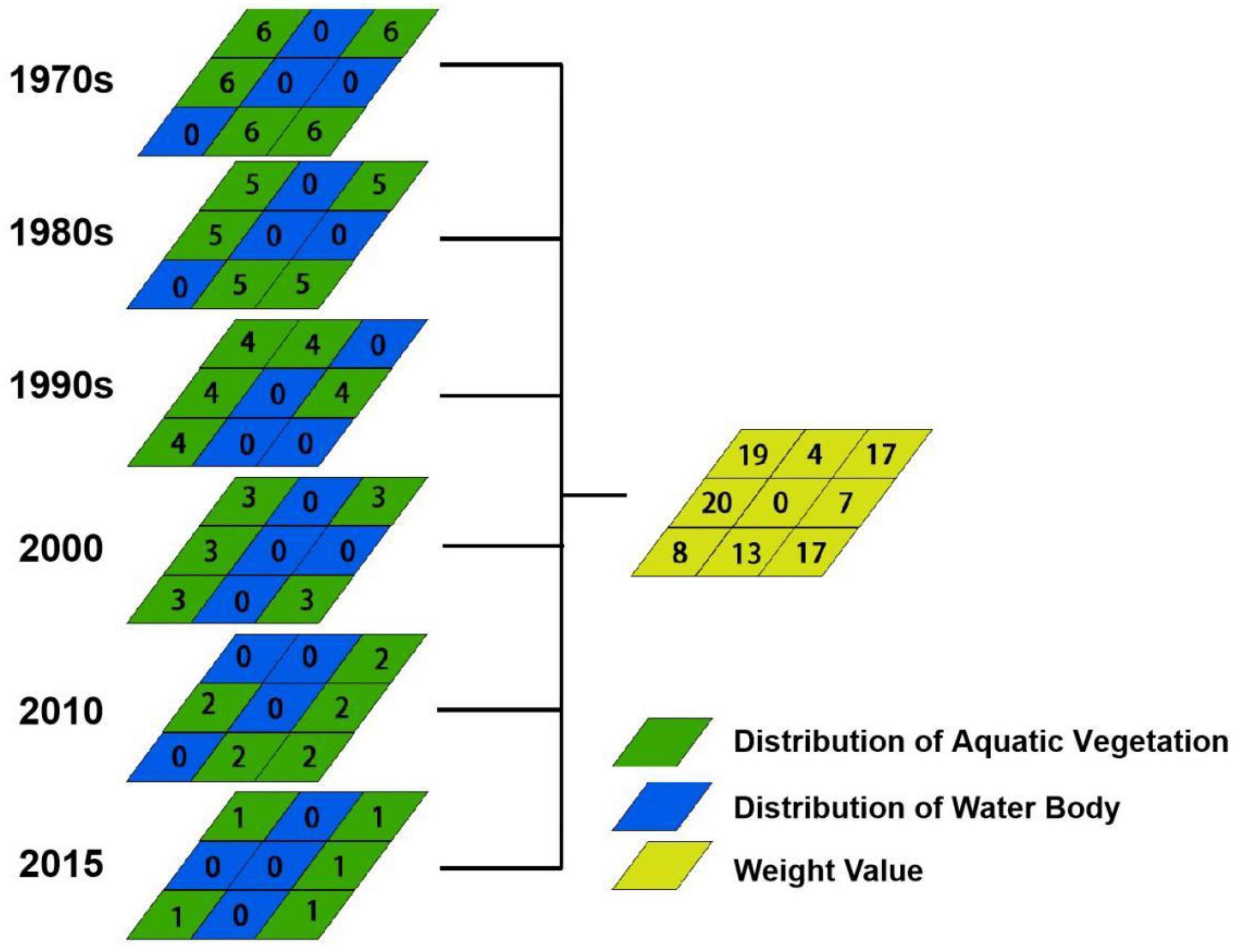
Figure 3. Temporal recency effect weighting analysis map of aquatic vegetation.

We normalized the weights of the spatial frequency of occurrence and the temporal recency effect and multiplied them to produce spatiotemporal restricted factor image datasets. Then, they were used to generate the transfer suitability image in the Markov process, which provided transfer rules for the reconstruction of the spatial distribution of aquatic vegetation through the CA-Markov model.

Validation of simulation accuracy

The simulation results were validated through the quantitative evaluation of the modeled results and the interpretation of remote sensing data. The kappa coefficient is an important metric for consistency testing, and it can often be used to assess the effectiveness of a measure of classification (Visser and de Nijs, 2006). Because the analysis was focused on aquatic vegetation, the lake water surface area is much larger than lake aquatic vegetation. The resulting high kappa coefficient for the waterbody reduces model accuracy. Therefore, the model simulation error rate (MSER) was used to validate the model accuracy. The calculation is as follows:

$MSER=\left|\frac{D_o-D_s}{D_o}\right|$

where D_o is the area of aquatic vegetation in the interpretation data and D_s is the area of aquatic vegetation in the simulation. Ideally, the value of MSER is 0, indicating that the simulated results are in agreement with the interpretation results.

In this study, a 5*5 filter was implemented in the improved CA-Markov model. This means that a rectangular space of 5*5 around a pixel was considered to have a significant influence on that the state change of the pixel (Zhao et al., 2011). The weight of each neighboring cell (i.e., pixel) was considered to have the same influence on the central cell. Since there were no spatial data on aquatic vegetation in Hulun Lake and Xingkai Lake in the 1950s and 1960s, it was difficult to validate the simulation results in these two periods. We used the improved CA-Markov model to simulate the distribution of the aquatic vegetation data in the 1990s and 1970s by 10-year steps and 20-year steps, respectively. Then, we validated the results of the simulation by comparing it with the interpretation of remote sensing data to calculate the kappa coefficient (He et al., 2020). The probability transfer matrix and the suitability image were two necessary parameters for the CA-Markov model to reconstruct the historical distribution. We considered the error transferability in order to simulate the spatial distribution of aquatic vegetation in the 1950s and 1960s, both of which were carried out based on the data from the 1970s. Moreover, the spatial distribution of aquatic vegetation in lakes in the 1950s and 1960s was reconstructed in 20-and 10-year steps, respectively. The CA-Markov model was implemented using IDRISI 17.0 software.

Results and analysis

Transfer probability matrix based on climate change consistency

The transfer probability matrix is a random matrix and is the basic quantity to characterize the Markov chain statistics, and it represents the linkage from one spatial characteristic to another (Fu et al., 2018). As the matrix describes independent spatial characteristics, their joint probability is the product of the probability measures of the two spaces separately (Eberly and Carlin, 2000). Therefore, the change in spatial distribution of aquatic vegetation from one period to another must correlate with spatiotemporal succession.

Meanwhile, a complex relationship was found between the changing pattern of aquatic vegetation and climatic conditions, which directly affected the distribution probability and transformation probability of aquatic vegetation in the lake. Therefore, the selection of suitable environmental factors can better simulate the dynamics of aquatic vegetation. According to related studies, there was a strong correlation between vegetation changes and meteorological factors in China, and the spatial distribution of aquatic vegetation also changed with climatic conditions. Consequently, we selected the annual average temperature and precipitation as environmental factors to assist the Markov model for calculating the probability transfer matrix.

Based on the meteorological data from the nearest weather stations around the lake during 1950–2015, the variation trends of annual average temperature and annual precipitation were analyzed at 20- and 10-year steps, respectively, to identify period with climate change trends similar to those of the 1950s and 1960s. Then, we used the Markov model to obtain the transfer probability matrix by superimposing the aquatic vegetation distribution map for those periods in the simulation reconstruction of aquatic vegetation in the 1950s and 1960s using IDRISI software. Figures 4–5 show the variation trends of annual mean temperature and annual rainfall in 20- and 10-year steps, respectively.

FIGURE 4

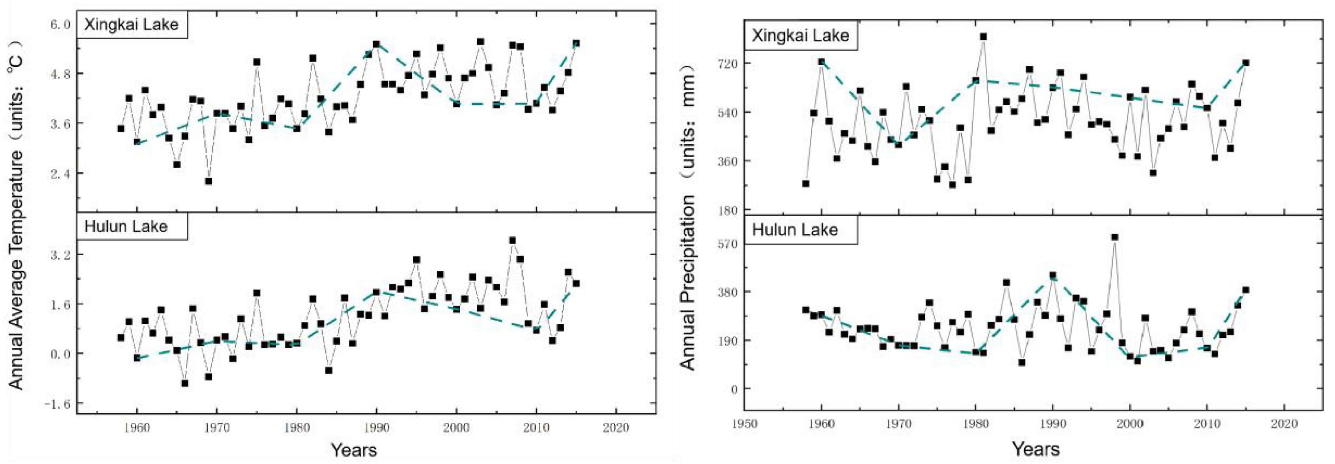
Figure 4. Variation trends per decade of annual average temperature (left) and annual precipitation data (right) during study periods.

FIGURE 5

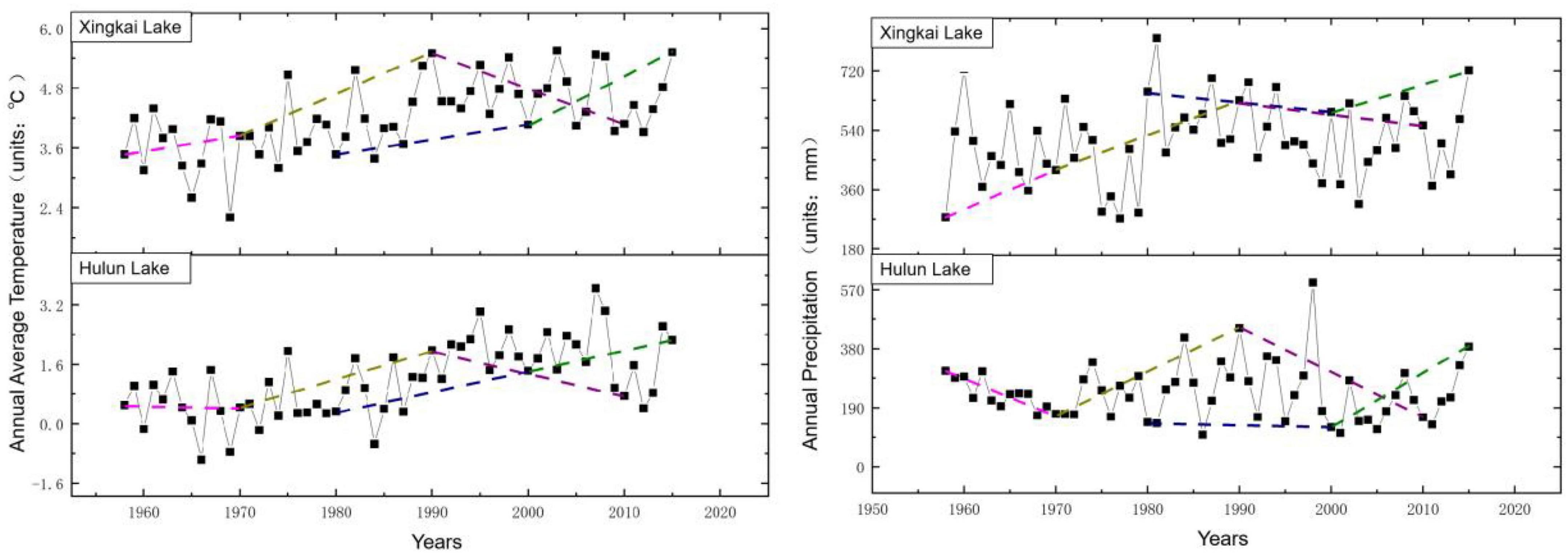
Figure 5. Variation trends per two decades of annual average temperature (left) and annual precipitation data (right) during study periods.

Considering the differences in the period of establishment of the weather stations and the period of acquiring the earliest meteorological data, we unified all the earliest meteorological data to 1958. Then, we fit the variation trends of annual mean temperature and annual rainfall in 20- and 10-year steps, respectively. Tables 3–4 show the fitted trends of temperature and precipitation for each period.

TABLE 3

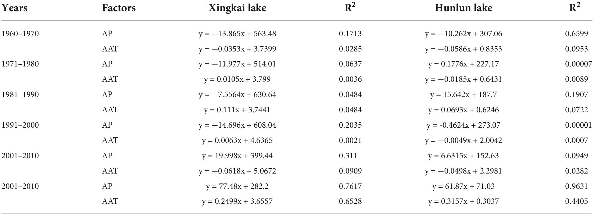
Table 3. Fitting equations for annual precipitation (AP) and annual average temperature (AAT) per decade.

TABLE 4

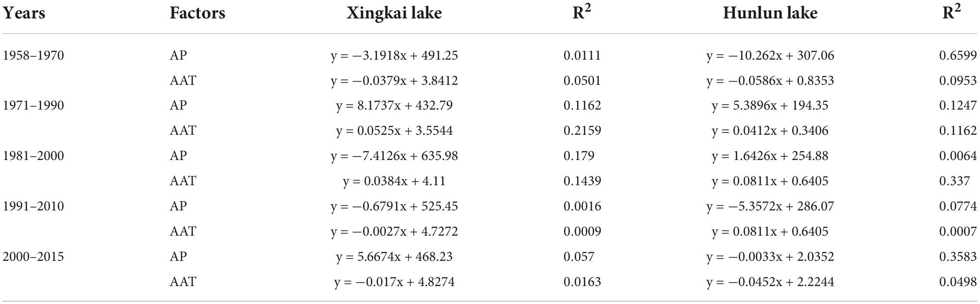
Table 4. Fitting equations for annual precipitation (AP) and annual average temperature (AAT) per two decades.

The variation trends of annual rainfall and average temperature of meteorological data of the two lakes were fitted by 10- and 20-year steps, respectively. Considering that temperature variation plays a key role in vegetation in North China, the period consistent with the temperature variation in the fitted time interval was selected as the basis for constructing the transfer probability matrix. For the simulation with a 10-year step, the variety of aquatic vegetation distribution data during 2001–2010 was selected as the calculated transfer probability matrix for the 1960–1970 fit. Uniformly, for the 20-year step, the change in aquatic vegetation distribution data from 2000 to 2015 was selected as the calculated transfer probability matrix for the 1950–1970 fit.

The reconstruction of historical data by the CA-Markov model is a reverse process that simulates past data using recent data. The calculation of the transfer probability matrix also occurs in the reverse direction. In order to simulate the distribution of aquatic vegetation in the 1960s with a 10-year step, we used the spatial distribution of aquatic vegetation from 2010 to 2000 to establish the transfer probability matrix extracted from the Markov model. Likewise, the transfer probability matrix for the 1950s with a 20-year step was established by the spatial distribution of aquatic vegetation from 2015 to 2000. The transfer probability matrices in the 1950s and 1960s were established using Markov models. Table 5 shows the parameters of transfer probability matrices in the CA-Markov model for predicting aquatic vegetation in the 1950s and 1960s.

TABLE 5

Table 5. Transfer probability matrices for predicting the 1950s and 1960s.

Construction of suitability images based on spatial frequency of occurrence and temporal recency effect

Based on the spatial frequency and temporal recency effect maps discussed earlier, we obtained the suitability images for aquatic vegetation adaptation by combining the weight analysis maps. The weight analysis maps obtained in the Markov process were combined with the Collection Editor to generate the transfer suitability images, and they provided the transfer rules for the reconstruction of the spatial distribution of aquatic vegetation by the CA-Markov model. Figure 6 shows the weight maps made by the spatial frequency of occurrence and temporal recency effect in Xingkai Lake, and Figure 7 shows the suitability image of Xingkai Lake.

FIGURE 6

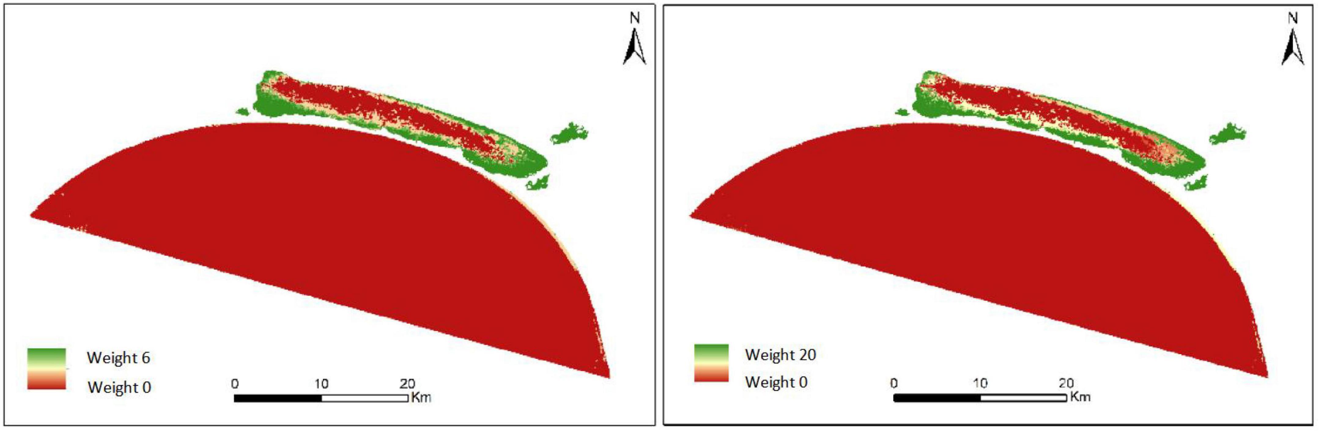
Figure 6. Weight analysis maps of the spatial frequency of occurrence (left) and temporal recency effect (right) in Xingkai Lake.

FIGURE 7

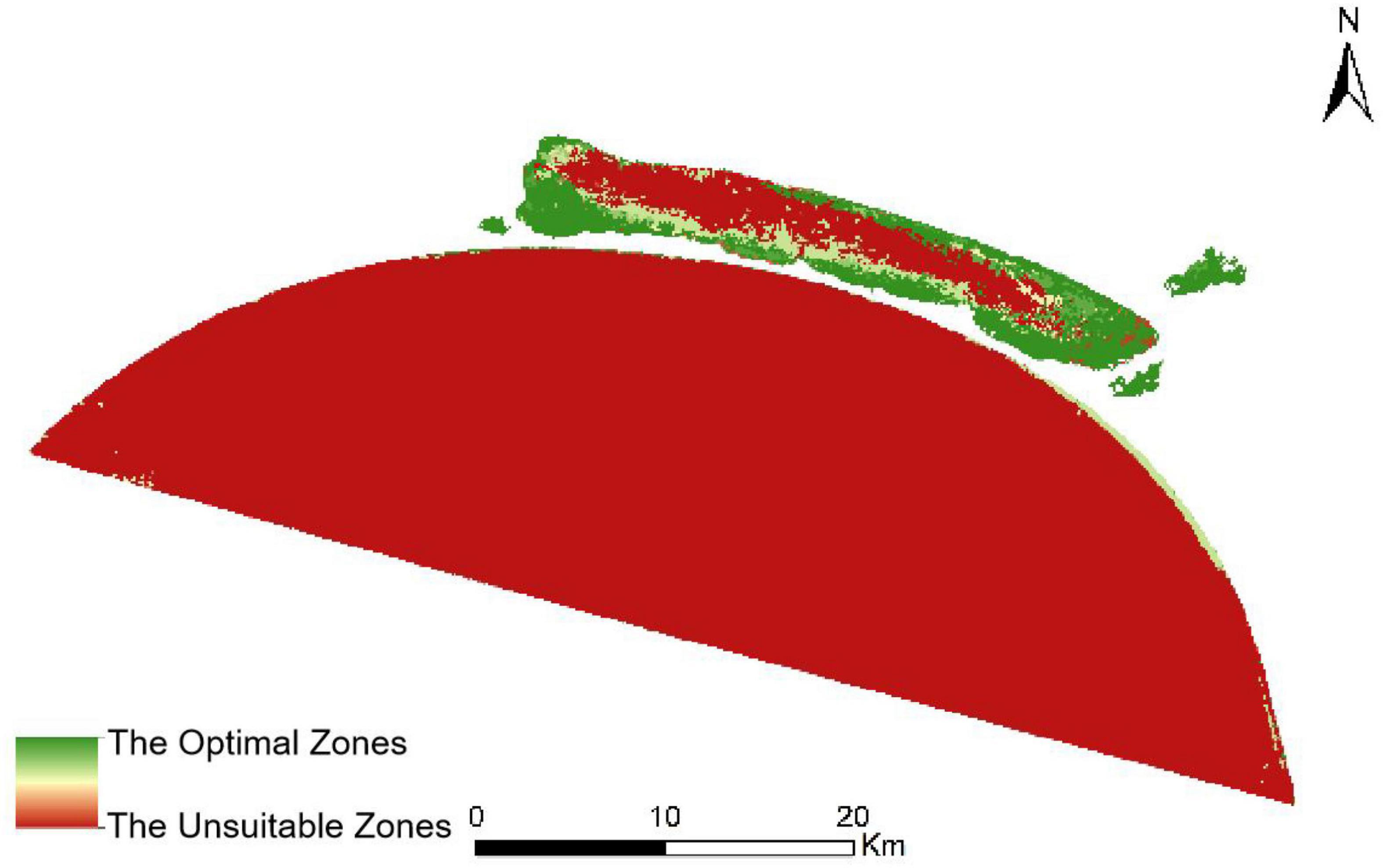
Figure 7. Suitability image of Xingkai Lake.

Simulation of the potential spatial distribution of aquatic vegetation in the 1950s and 1960s

Using the transfer probability matrix and suitability images, we implemented an improved CA-Markov model to reconstruct the potential spatial distribution of aquatic vegetation in the 1950s and 1960s with 20- and 10-year steps for Xingkai Lake and Hulun Lake. Figure 8 shows the spatial distribution of aquatic vegetation for the two lakes, while Table 6 shows the areas of aquatic vegetation in the lakes in the 1950s and 1960s.

FIGURE 8

Figure 8. Potential spatial distribution of aquatic vegetation in Xingkai Lake and Hulun Lake in the 1950s and 1960s.

TABLE 6

Table 6. Areas of aquatic vegetation in Xingkai Lake and Hulun Lake in the 1950s and 1960s (km²).

The area of aquatic vegetation in Xingkai Lake was 102.37 km² in the 1950s, 100.70 km² in the 1960s, and 61.64 km² in the 1970s, showing a decreasing trend in aquatic vegetation areas. For Hulun Lake, the area of aquatic vegetation was 90.81 km² in the 1950s, 88.15 km² in the 1960s, and 60.87 km² in the 1970s. This also shows a decreasing trend in the area of aquatic vegetation, which is consistent with the results of the study by Zhang et al. (2019).

Discussion and conclusion

Discussion

Simulation accuracy

Due to the lack of ground survey data in the 1950s and 1960s and the absence of relevant thematic maps and remote sensing images, it was difficult to verify the simulated spatial distributions of aquatic vegetation in the two lakes. To determine the effect of the improved CA-Markov model, we compared the effects of the traditional CA-Markov model and the improved model (He et al., 2020). The spatial distribution of aquatic vegetation in the two lakes in the 1980s was simulated using the traditional and improved models in 10- and 20-year steps, respectively. Then, we compared the results of the two models with interpretations of the aquatic vegetation distribution from remote sensing images in order to evaluate the reliability and accuracy of the improved CA-Markov model.

First, we implemented the evaluation in 10-year steps. The distributions of aquatic vegetation of the two lakes in the 1990s were used as base data to simulate the probable distribution of aquatic vegetation in the 1980s by using the traditional and improved CA-Markov models. The traditional model was obtained from the transfer probability matrix based on the characteristics of aquatic vegetation changes in the lakes from 2000 to 1990; simulation directly applied the CA-Markov model method without considering geographical factors. We used the approach presented in this article to construct simulation rules for an improved CA-Markov model to simulate the distribution of aquatic vegetation in the 1980s. Table 7 shows the MSER of the accuracy comparison between the results of the two models and the interpretation result.

TABLE 7

Table 7. Comparison of results of the traditional CA-Markov model and improved CA-Markov model with 10-year steps.

Table 7 shows that the improved CA-Markov model was used to simulate the distribution of the aquatic vegetation of Xingkai Lake in the 1980s, and the simulation accuracy was improved by 64.86% compared with that in the traditional CA-Markov model. However, the results of the improved CA-Markov model were inferior to the traditional CA-Markov model in MSER indicators in Hulun Lake. This is because the results of the traditional model simulated the distribution pattern of aquatic vegetation on the western shore of the lake, which is closer to the remote sensing extraction results. Figure 9 shows the comparison between the interpretation results and the simulation results of the two models.

FIGURE 9

Figure 9. Comparison between the interpretation results and the simulation results of two models with a 10-year step (A: results of the traditional CA-Markov model; B: results of the improved CA-Markov model; C: results of interpretation remote sensing).

We also implemented the evaluation with a 20-year step. The distribution of the aquatic vegetation of the two lakes in the 1990s was used as base data to simulate the probable distribution of the 1980s using the traditional and improved models. Table 8 shows the MSER of the accuracy comparison between the results of the two models and the interpretation results.

TABLE 8

Table 8. Comparison of results of the traditional CA-Markov model and improved CA-Markov model with 20-year steps.

Table 8 shows the comparison of results of the traditional and improved CA-Markov models with 20-year steps. In the reconstructed historical data, the results of the improved CA-Markov model are significantly better for Xingkai Lake and Hulun Lake. The MSER value of the traditional CA-Markov model increased significantly: the MSER of the traditional model result of Xingkai Lake reached 1.61, while the MSER of the improved model was 0.79, improving by 51.34%. Overall model accuracy improved by more than 52% for the 20-year step with the improved CA-Markov model. Therefore, the improved CA-Markov model must be supported by geographical data for better simulation under longer term simulation conditions. Figure 10 shows the comparison between the interpretation results and the simulation results of the two models.

FIGURE 10

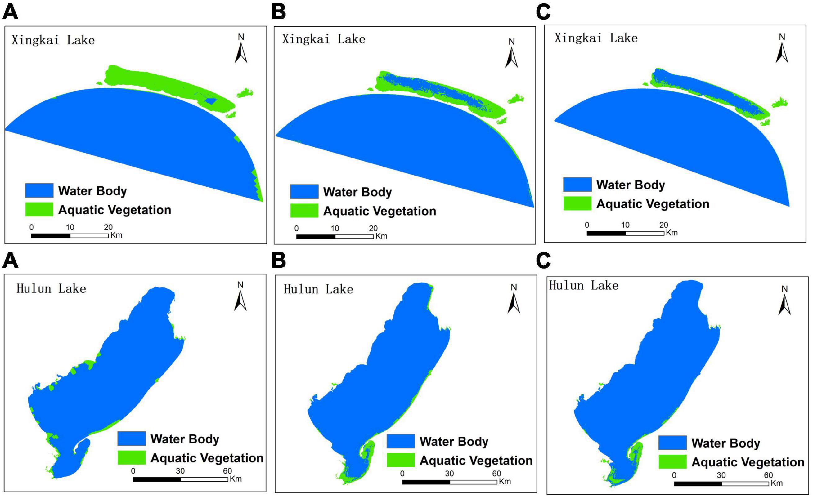
Figure 10. Comparison between the interpretation results and the simulation results of the two models with a 20-year step (A: results of the traditional CA-Markov model; B: results of the improved CA-Markov model; C: results of interpretation remote sensing).

By improving the CA-Markov model, we provided a new simulation of the potential distribution of aquatic vegetation in the historical period. The results of the improved model had higher accuracy than the results of the traditional CA-Markov model. The transfer probability matrix of the improved CA-Markov model was constructed based on the consistency of changes in environmental conditions (meteorological factors), and then it was combined with a spatial frequency of occurrence and temporal recency effect to enhance the rules for suitability images. This improved model represents a rigorous method for the simulation and reconstruction of aquatic vegetation information in historical periods. In addition, it provided a reference for the reconstruction of the historical spatial distributions of other features.

Implications for reconstruction

To the best of our knowledge, the CA-Markov model has been widely used for the surface type changes in feature prediction and historical reconstruction (Yang et al., 2021; He et al., 2022). Although many studies have focused on qualitative methods for the suitability of images, it has not improved since the 1980s (Fu et al., 2018). Particularly, the selection of constraint factors for the suitability images neglected the connection to local historical spatiotemporal data, and we argued that the historical data were important factors for the inter-decadal succession of plant growth.

This study has made several innovative contributions to the literature. First, although the CA-Markov model has been widely used to reconstruct land cover patterns in historical periods (Yang et al., 2016), this is the first study to examine the historical distribution of the aquatic vegetation in lakes. In particular, our approach compensates for the difficulty of obtaining datasets due to the absence of historical remote sensing images and maps; such datasets are important for studying the evolution of lake ecosystems.

Second, we attempt to identify periods with similar climate change trends in different histories. We determine the transition probability matrix based on the distribution of aquatic vegetation in these periods. The aforementioned evaluation shows that our approach successfully improves simulation accuracy.

Third, historical reconstruction is a reverse process in which the past state is simulated from the current state. Therefore, the transfer probability matrix must be constructed from the current to the historical state. This finding provides new insights for the historical simulation of other relevant land surface types.

Fourth, the influencing factors of the spatiotemporal succession of vegetation growth were included as restrictive conditions in the model. Unlike the simulation of land-use types, human activities and policies have a large impact on prediction and reconstruction of land-use cover changes (Fu et al., 2018; Zhang et al., 2020), while the spatiotemporal succession of aquatic vegetation is important for sustainability over long timescales. In this study, we selected the spatial occurrence frequency and temporal recency effect of aquatic vegetation growth as the two most important constraint factors to generate the suitability images. These images, in turn, controlled the transformation process of the cellular automata in the model.

Finally, we selected two typical lakes in Northeast China to reconstruct the historical distribution of the aquatic vegetation. Due to the large number of lakes in China, most of them lack historical records. Therefore, reconstructing the historical spatial distribution of aquatic vegetation is significant for studying the response of lake ecosystems to global climate change. The methodology and reconstruction process in this study can provide a reference model for other lakes.

Limitation for applicability

The improved CA-Markov model not only enriches the method of estimating historical aquatic vegetation but also provides a scientific basis for the response of lake ecosystems to climate change in China. Although we successfully reconstructed potential spatial distributions using the improved CA-Markov model, a few uncertainties and limitations remain. First, suitability images were constructed using spatial distribution data on aquatic vegetation in six periods (1970–2015). Because of the reconstruction of the historical spatial distribution of aquatic vegetation, the spatial distributions extracted from remote sensing data in all six periods were used in the simulation process. Thus, the results of the aquatic vegetation simulation were obtained in every possible distribution area. In addition, aquatic vegetation change is a complex process influenced not only by natural factors, such as climate change and natural disasters, but also by uncertain factors such as socioeconomic development and other human activities. The problem of setting the parameters of the CA-Markov model while considering such factors should be explored in future research.

Conclusion

This article proposes an improved CA-Markov model to reconstruct the spatial distribution of feature elements in historical periods. The model is based on the reverse transfer probability matrix derived from changes in meteorological factors and suitability images calculated from the spatial frequency of occurrence and the temporal recency effect. The main conclusions obtained are as follows:

(1) The transfer probability matrix is constructed based on the consistency of changes in meteorological elements and the cell conversion rules established from the climate-driven perspective, providing a theoretical basis for the simulation of the spatial distribution of aquatic vegetation.

(2) The suitability images are constructed from the spatial frequency of occurrence and the temporal recency effect, further standardizing the constraints and influences from the spatiotemporal correlation of geographic elements; this makes the simulation results of the model more convincing.

(3) The spatial distribution of aquatic vegetation in the 1990s is simulated and validated for consistency with the results of remote sensing image interpretation. The improved CA-Markov model has good generalizability for simulating the potential spatial distribution of historical aquatic vegetation.

Data availability statement

The original contributions presented in this study are included in the article/supplementary material, further inquiries can be directed to the corresponding author.

Author contributions

GH and HZ designed the study and completed the manuscript. ZL revised the manuscript. HZ, ZC, and YC contributed to the data collection and processing. All authors have read and agreed to the published version of the manuscript.

Funding

This work was financially supported by the National Key Research and Development Program of China (2019YFA0607101 and 2021YFD1500104) and the National Natural Science Foundation of China (41701494).

Conflict of interest

The authors declare that the research was conducted in the absence of any commercial or financial relationships that could be construed as a potential conflict of interest.

Publisher’s note

All claims expressed in this article are solely those of the authors and do not necessarily represent those of their affiliated organizations, or those of the publisher, the editors and the reviewers. Any product that may be evaluated in this article, or claim that may be made by its manufacturer, is not guaranteed or endorsed by the publisher.

Footnotes

1. ^ http://www.gscloud.cn/
2. ^ http://data.cma.cn/

References

Aaviksoo, K. (1993). Changes of plant cover and land use types (1950’s to 1980’s) in three mire reserves and their neighbourhood in Estonia. Landsc. Ecol. 8, 287–301. doi: 10.1007/BF00125134

CrossRef Full Text | Google Scholar

Ahmed, B. (2011). Modelling spatio-temporal urban land cover growth dynamics using remote sensing and GIS techniques: A case study of Khulna City. J. Bangladesh Inst. Plann. 4:43.

Google Scholar

Bilton, D. T., Mcabendroth, L., Bedford, A., and Ramsay, P. M. (2006). How wide to cast the net? Cross-taxon congruence of species richness, community similarity and indicator taxa in ponds. Freshw. Biol. 51, 578–590. doi: 10.1111/j.1365-2427.2006.01505.x

CrossRef Full Text | Google Scholar

Bu, H., Wan, J., Zhang, Y., and Meng, W. (2013). Spatial characteristics of surface water quality in the Haicheng River (Liao River basin) in Northeast China. Environ. Earth Sci. 70, 2865–2872. doi: 10.1007/s12665-013-2348-5

CrossRef Full Text | Google Scholar

Dai, L., Liu, Y., and Luo, X. (2021). Integrating the MCR and DOI models to construct an ecological security network for the urban agglomeration around Poyang Lake, China. Sci. Total Environ. 754:141868. doi: 10.1016/j.scitotenv.2020.141868

PubMed Abstract | CrossRef Full Text | Google Scholar

Eberly, L. E., and Carlin, B. P. (2000). Identifiability and convergence issues for Markov chain Monte Carlo fitting of spatial models. Stat. Med. 19, 2279–2294. doi: 10.1002/1097-0258(20000915/30)19:17/18<2279::aid-sim569>3.0.co;2-r

PubMed Abstract | CrossRef Full Text | Google Scholar

Fornes, A., Basterretxea, G., Orfila, A., Jordi, A., Alvarez, A., and Tintore, J. (2006). Mapping Posidonia oceanica from IKONOS. ISPRS J. Photogramm. Remote Sens. 60, 315–322. doi: 10.1016/j.isprsjprs.2006.04.002

CrossRef Full Text | Google Scholar

Fu, F., Deng, S., Wu, D., Liu, W., and Bai, Z. (2022). Research on the spatiotemporal evolution of land use landscape pattern in a county area based on CA-Markov model. Sustain. Cities Soc. 80:103760. doi: 10.1016/j.scs.2022.103760

CrossRef Full Text | Google Scholar

Fu, X., Wang, X., and Yang, Y. J. (2018). Deriving suitability factors for CA-Markov land use simulation model based on local historical data. J. Environ. Manage. 206, 10–19. doi: 10.1016/j.jenvman.2017.10.012

PubMed Abstract | CrossRef Full Text | Google Scholar

Getachew, B., Manjunatha, B. R., and Bhat, H. G. (2021). Modeling projected impacts of climate and land use/land cover changes on hydrological responses in the Lake Tana Basin, upper Blue Nile River Basin, Ethiopia. J. Hydrol. 595:125974. doi: 10.1016/j.jhydrol.2021.125974

CrossRef Full Text | Google Scholar

He, F., Yang, J., Zhang, Y., Sun, D., Wang, L., Xiao, X., et al. (2022). Offshore Island connection line: A new perspective of coastal urban development boundary simulation and multi-scenario prediction. GIsci Remote Sens. 59, 801–821. doi: 10.1080/15481603.2022.2071056

CrossRef Full Text | Google Scholar

He, Z. S. Y., Xie, L., Liang, B. P., Deng, X. J., Yan, T. Q., Tong, Y. J., et al. (2020). Simulation of land use in Li River Basin based on CA-Markov model. Ecol. Sci. 39, 142–150. doi: 10.14108/j.cnki.1008-8873.2020.05.017

CrossRef Full Text | Google Scholar

Horppila, J., and Nurminen, L. (2003). Effects of submerged macrophytes on sediment resuspension and internal phosphorus loading in Lake Hiidenvesi (southern Finland). Water Res. 37, 4468–4474. doi: 10.1016/S0043-1354(03)00405-6

CrossRef Full Text | Google Scholar

Jeppesen, E., Lauridsen, T., Kairesalo, T., and Perrow, M. (1998). “Impact of submerged macrophytes on fish-zooplankton interactions in lakes,” in The structuring role of submerged macrophytes in lakes, eds E. Jeppesen, M. Søndergaard, and K. Christoffersen (New York, NY: Springer).

Google Scholar

Kolada, A., Willby, N., Dudley, B., Nõges, P., Søndergaard, M., Hellsten, S., et al. (2014). The applicability of macrophyte compositional metrics for assessing eutrophication in European lakes. Ecol. Indic. 45, 407–415. doi: 10.1016/j.ecolind.2014.04.049

CrossRef Full Text | Google Scholar

Körner, S., and Nicklisch, A. (2002). Allelopathic growth inhibition of selected phytoplankton species by submerged macrophytes. J. Phycol. 38, 862–871. doi: 10.1046/j.1529-8817.2002.t01-1-02001.x

CrossRef Full Text | Google Scholar

Laba, M., Blair, B., Downs, R., Monger, B., Philpot, W., Smith, S., et al. (2010). Use of textural measurements to map invasive wetland plants in the Hudson River National Estuarine Research Reserve with IKONOS satellite imagery. Remote Sens. Environ. 114, 876–886. doi: 10.1016/j.rse.2009.12.002

CrossRef Full Text | Google Scholar

Lee, G. K. L., and Chan, E. H. W. (2008). The analytic hierarchy process (AHP) approach for assessment of urban renewal proposals. Soc. Indic. Res. 89, 155–168. doi: 10.1007/s11205-007-9228-x

CrossRef Full Text | Google Scholar

Liira, J., Feldmann, T., Mäemets, H., and Peterson, U. (2010). Two decades of macrophyte expansion on the shores of a large shallow northern temperate lake–A retrospective series of satellite images. Aquat. Bot. 93, 207–215. doi: 10.1016/j.aquabot.2010.08.001

CrossRef Full Text | Google Scholar

Luo, Z., Feng, W., Luo, Y., Baldock, J., and Wang, E. (2017). Soil organic carbon dynamics jointly controlled by climate, carbon inputs, soil properties and soil carbon fractions. Glob. Chang. Biol. 23, 4430–4439. doi: 10.1111/gcb.13767

PubMed Abstract | CrossRef Full Text | Google Scholar

Mao, P., Zhang, J., Li, M., Liu, Y., Wang, X., Yan, R., et al. (2022). Spatial and temporal variations in fractional vegetation cover and its driving factors in the Hulun Lake region. Ecol. Indic. 135:108490. doi: 10.1016/j.ecolind.2021.108490

CrossRef Full Text | Google Scholar

Mondal, M. S., Sharma, N., Garg, P. K., and Kappas, M. (2016). Statistical independence test and validation of CA Markov land use land cover (LULC) prediction results. Egypt. J. Remote. Sens. Space Sci. 19, 259–272. doi: 10.1016/j.ejrs.2016.08.001

CrossRef Full Text | Google Scholar

Moss, B., Kosten, S., Meerhoff, M., Battarbee, R. W., Jeppesen, E., Mazzeo, N., et al. (2011). Allied attack: Climate change and eutrophication. Inland Waters 1, 101–105. doi: 10.5268/IW-1.2.359

CrossRef Full Text | Google Scholar

Orth, R. J., Carruthers, T. J. B., Dennison, W. C., Duarte, C. M., Fourqurean, J. W., Heck, K. L., et al. (2006). A global crisis for seagrass ecosystems. Bioscience 56, 987–996.

Google Scholar

Qing, S., Runa, A., Shun, B., Zhao, W., Bao, Y., and Hao, Y. (2020). Distinguishing and mapping of aquatic vegetations and yellow algae bloom with landsat satellite data in a complex shallow lake, China during1986-2018. Ecol. Indic. 112:106073. doi: 10.1016/j.ecolind.2020.106073

CrossRef Full Text | Google Scholar

Roijackers, R., Szabó, S., and Scheffer, M. (2004). Experimental analysis of the competition between algae and duckweed. Arch. Hydrobiol. 160, 401–412. doi: 10.1127/0003-9136/2004/0160-0401

CrossRef Full Text | Google Scholar

Sand-Jensen, K., Riis, T., Vestergaard, O., and Larsen, S. E. (2000). Macrophyte decline in danish lakes and streams over the past 100 years. J. Ecol. 88, 1030–1040. doi: 10.1046/j.1365-2745.2000.00519.x

CrossRef Full Text | Google Scholar

Sang, L., Zhang, C., Yang, J., Zhu, D., and Yun, W. (2011). Simulation of land use spatial pattern of towns and villages based on CA–Markov model. Math. Comput. Simul. 54, 938–943. doi: 10.1016/j.mcm.2010.11.019

CrossRef Full Text | Google Scholar

Song, K., Shang, Y., Wen, Z., Jacinthe, P.-A., Liu, G., Lyu, L., et al. (2019). Characterization of CDOM in saline and freshwater lakes across China using spectroscopic analysis. Water Res. 150, 403–417. doi: 10.1016/j.watres.2018.12.004

PubMed Abstract | CrossRef Full Text | Google Scholar

Visser, H., and de Nijs, T. (2006). The map comparison kit. Environ. Model. Softw. 21, 346–358. doi: 10.1016/j.envsoft.2004.11.013

CrossRef Full Text | Google Scholar

Wang, S., Meng, W., Jin, X., Zheng, B., Zhang, L., and Xi, H. (2015). Ecological security problems of the major key lakes in China. Environ. Earth Sci. 74, 3825–3837. doi: 10.1007/s12665-015-4191-3

CrossRef Full Text | Google Scholar

Wang, Y., Shen, X., Jiang, M., and Lu, X. (2020). Vegetation change and its response to climate change between 2000 and 2016 in marshes of the Songnen plain, Northeast China. Sustainability 12:3569. doi: 10.3390/SU12093569

CrossRef Full Text | Google Scholar

Yang, J., Guo, A., Li, Y., Zhang, Y., and Li, X. (2019). Simulation of landscape spatial layout evolution in rural-urban fringe areas: A case study of Ganjingzi District. GIsci Remote Sens. 56, 388–405. doi: 10.1080/15481603.2018.1533680

CrossRef Full Text | Google Scholar

Yang, J., Yang, R., Chen, M.-H., Su, C.-H., Zhi, Y., and Xi, J. (2021). Effects of rural revitalization on rural tourism. J. Hosp. Tour. Manag. 47, 35–45. doi: 10.1016/j.jhtm.2021.02.008

CrossRef Full Text | Google Scholar

Yang, X., Jin, X., Du, X., Xiang, X., Han, J., Shan, W., et al. (2016). Multi-agent model-based historical cropland spatial pattern reconstruction for 1661–1952, Shandong Province, China. Glob. Planet. Change 143, 175–188. doi: 10.1016/j.gloplacha.2016.06.010

CrossRef Full Text | Google Scholar

Yuan, Y., Jiang, M., Liu, X., Yu, H., Otte, M. L., Ma, C., et al. (2018). Environmental variables influencing phytoplankton communities in hydrologically connected aquatic habitats in the Lake Xingkai basin. Ecol. Indic. 91, 1–12. doi: 10.1016/j.ecolind.2018.03.085

CrossRef Full Text | Google Scholar

Zavadskas, E. K., and Antucheviciene, J. (2007). Multiple criteria evaluation of rural building’s regeneration alternatives. Build Environ. 42, 436–451. doi: 10.1016/j.buildenv.2005.08.001

CrossRef Full Text | Google Scholar

Zhang, G., Yao, T., Chen, W., Zheng, G., Shum, C. K., Yang, K., et al. (2019). Regional differences of lake evolution across China during 1960s–2015 and its natural and anthropogenic causes. Remote Sens. Environ. 221, 386–404. doi: 10.1016/j.rse.2018.11.038

CrossRef Full Text | Google Scholar

Zhang, X., Zhou, J., and Li, M. (2020). Analysis on spatial and temporal changes of regional habitat quality based on the spatial pattern reconstruction of land use. Acta Geogr. Sin. 75, 160–178. doi: 10.11821/dlxb202001012

CrossRef Full Text | Google Scholar

Zhao, G. W., Chen, Y. B., Chen, J. F., and Li, J. T. (2011). Spatial scale sensitivity of CA-Markov model. Sci. Geol. Sin. 31, 897–902. doi: 10.13249/j.cnki.sgs.2011.08.014

CrossRef Full Text | Google Scholar

Zhao, Q. Q., Zhang, J. P., Zhao, T. B., and Li, J. H. (2021). Vegetation changes and its response to climate change in China since 2000. Plateau Meteorol. 40, 292–301. doi: 10.7522/j.issn.1000-0534.2020.00025

CrossRef Full Text | Google Scholar

Zhou, L., Dang, X., Sun, Q., and Wang, S. (2020). Multi-scenario simulation of urban land change in Shanghai by random forest and CA-Markov model. Sustain. Cities Soc. 55:102045. doi: 10.1016/j.scs.2020.102045

CrossRef Full Text | Google Scholar