 Marina D. A. Scarpelli
 Benoit Liquet2,3
 Susan Fuller
 Paul Roe
- 1Faculty of Science, Queensland University of Technology, Brisbane, QLD, Australia
- 2Department of Mathematics and Statistics, Macquarie University, Sydney, NSW, Australia
- 3CNRS, Laboratoire de Mathématiques et de leurs Applications de PAU E2S UPPA, Pau, France
High rates of biodiversity loss caused by human-induced changes in the environment require new methods for large scale fauna monitoring and data analysis. While ecoacoustic monitoring is increasingly being used and shows promise, analysis and interpretation of the big data produced remains a challenge. Computer-generated acoustic indices potentially provide a biologically meaningful summary of sound, however, temporal autocorrelation, difficulties in statistical analysis of multi-index data and lack of consistency or transferability in different terrestrial environments have hindered the application of those indices in different contexts. To address these issues we investigate the use of time-series motif discovery and random forest classification of multi-indices through two case studies. We use a semi-automated workflow combining time-series motif discovery and random forest classification of multi-index (acoustic complexity, temporal entropy, and events per second) data to categorize sounds in unfiltered recordings according to the main source of sound present (birds, insects, geophony). Our approach showed more than 70% accuracy in label assignment in both datasets. The categories assigned were broad, but we believe this is a great improvement on traditional single index analysis of environmental recordings as we can now give ecological meaning to recordings in a semi-automated way that does not require expert knowledge and manual validation is only necessary for a small subset of the data. Furthermore, temporal autocorrelation, which is largely ignored by researchers, has been effectively eliminated through the time-series motif discovery technique applied here for the first time to ecoacoustic data. We expect that our approach will greatly assist researchers in the future as it will allow large datasets to be rapidly processed and labeled, enabling the screening of recordings for undesired sounds, such as wind, or target biophony (insects and birds) for biodiversity monitoring or bioacoustics research.
Introduction
Biodiversity loss is a global environmental issue (Cardinale et al., 2012), and it is now imperative to develop methods to efficiently monitor wildlife, accounting for spatial and temporal coverage (Joppa et al., 2016). Remote sensing techniques are being used to fill this gap, as they can be applied over large geographic areas where access may be difficult, allowing for some degree of unattended monitoring (Kerr and Ostrovsky, 2003). Remote sensing techniques include a range of technologies, like satellite imaging (Bonthoux et al., 2018), camera traps (Fontúrbel et al., 2021), Unmanned Aerial Vehicles (UAVs) (Nowak et al., 2019), and passive acoustic monitoring (PAM) (Froidevaux et al., 2014; Wrege et al., 2017).
Passive acoustic monitoring is now routinely used in terrestrial environments to monitor biodiversity (Gibb et al., 2019) with several purposes, such as understanding acoustic community composition of frog choruses (Ulloa et al., 2019), investigating acoustic species diversity of different taxonomic groups (Aide et al., 2017), and bird species recognition based on syllable recognition (Petrusková et al., 2016). Long-term recording can enable detection of species responses to important environmental impacts like climate change (Krause and Farina, 2016), and species recovery following extreme weather events (Duarte et al., 2021). However, recordings comprise large datasets which can be challenging to store, access and analyze (Ulloa et al., 2018). Subsampling is one way of dealing with these constraints, but it can limit the temporal and/or spatial scale of monitoring, therefore methods to analyze and filter recordings are necessary.
Currently, analysis of acoustic recordings still heavily relies on manual listening and inspection of recordings: this greatly limits the applicability of PAM. One alternative to that is to summarize acoustic information using acoustic indices, which mathematically represent different aspects of sound (e.g., frequency, intensity, etc.) (Sueur et al., 2014). Acoustic indices have, in some cases, been inspired by ecological indices. For example, the acoustic diversity index (Villanueva-Rivera et al., 2011) is based on the Shannon diversity index (Shannon and Weaver, 1964). NDSI (Gage and Axel, 2014) measures the ratio between biophony (biological sounds) and anthrophony (human and technological sounds) and is derived from NDVI, an index used in the remote sensing analysis of vegetation (Pettorelli, 2013). Acoustic indices have been used in different contexts such as to evaluate the differences in faunal beta-diversity between forests and plantations (Hayashi et al., 2020), to detect rainfall in acoustic recordings (Sánchez-Giraldo et al., 2020), to examine differences among indices representing taxonomic groups (e.g., birds, anurans, mammals and insects) (Ferreira et al., 2018), to relate indices with bird diversity (Tucker et al., 2014), and to identify frog species (Brodie et al., 2020).
Although there are numerous acoustic indices to choose from, different indices represent different acoustic phenomena in terrestrial environments, and the translation of acoustic into ecological information may vary depending on the context (Machado et al., 2017; Jorge et al., 2018; Bradfer-Lawrence et al., 2020). While there is no consensus on linking one index to one taxa, research has shown that combining indices can provide a good representation of different soundscapes (i.e., sounds in the landscape), especially across varying environments (Towsey et al., 2018), and can even be used to recognize different species (Brodie et al., 2020). Visualization tools such as false-color spectrograms (FCS) successfully combine three acoustic indices [Acoustic Complexity Index (Pieretti et al., 2011), Temporal Entropy (Sueur et al., 2008) and Events per Second (Towsey, 2018)] allowing different sound sources to be identified. The FCS and its combination of indices have been shown to provide a good representation of soundscapes in different contexts (e.g., Brodie et al., 2020; Znidersic et al., 2020). While visual representations of soundscapes are useful for scanning recordings for different phenomena (like rain, wind, or a frog chorus, for example), there is currently no available tool to statistically analyze these images. The underlying index data used to create the FCS can be retrieved and analyzed, but the mathematical interpretation of multiple indices remains a challenge, and therefore the statistical analysis of single indices is currently the favored approach. If mass deployments are required, [e.g., Australian Acoustic Observatory—(Roe et al., 2021)], we need to develop reliable, reproducible analysis methods with some degree of automation.
Furthermore, most statistical methods used for continuous recordings require an approach that accounts for temporal autocorrelation of the data (i.e., most statistical tests applied in ecology require independence of data). This means that each minute is not independent of the previous one in a recording, and this is often ignored in ecoacoustic studies. While spatial autocorrelation can be dealt with through experimental design, temporal correlation exists even when data are non-continuous (e.g., subsampled for example 1 min every 15 min) or arbitrarily split into time periods (e.g., day/night). Standard statistical approaches which assume independence of data cannot be applied for autocorrelated data.
Aiming to address the different challenges faced by researchers when analyzing recordings, we present a novel workflow for analyzing multi-index acoustic data. Our goal was to provide a tool that can be used by ecologists in a rapid assessment of terrestrial acoustic recordings. By having such a tool, ecologists can forward recordings of interest (i.e., for species identification) to specialists more efficiently, but also have quick metrics to compare ecosystems and/or recordings from different points in time. To deal with autocorrelated data capturing repeated patterns in acoustic indices is an alternative. Using the Hierarchical Based Motif Enumeration (HIME) (Gao and Lin, 2017) of acoustic indices, repetitive patterns of the data were detected (here referred to as motifs) in continuous recordings. As the algorithm searches for repetition of patterns in the time-series (Zolhavarieh et al., 2014) it was expected that noisy minutes (i.e., non-signal) would be excluded from the results as they tend to be random and not have a structure that repeats across time. Here we outline a semi-supervised method to classify the motifs according to dominant sounds. We demonstrate the transferability of the analysis in different environments and timescales with two case studies using data from two distinct ecosystems and recorded with different sampling schemes and devices.
Materials and Methods
Acoustic Analysis
The recordings were analyzed using AnalysisPrograms.exe (Towsey et al., 2020) three indices were used to create FCS (Towsey et al., 2014). These indices are: (1) Acoustic Complexity – quantification of relative changes in amplitude (Pieretti et al., 2011); (2) Temporal Entropy – concentration of energy overall the amplitude envelope (Sueur et al., 2008); (3) Events Per Second – number of acoustic events that exceeds 3dB per second (Towsey, 2018). FCS have been used successfully to represent a range of different soundscapes (Brodie et al., 2020; Gan et al., 2020; Indraswari et al., 2020; Znidersic et al., 2020), and provide a visual tool to aid in the identification of sounds, reducing the time required for verification of data.
The analysis was done directly on the unprocessed recordings, meaning that no noise (unwanted sounds) was removed beforehand. Acoustic data will have different sound sources and the presence of noise is common. Moreover, pre-processing can be time consuming, and so we tested the method without any type of pre-processing (i.e., cleaning up) of the data.
All analyses were performed using R and scripts are available at http://doi.org/10.5281/zenodo.4784758 (Scarpelli, 2021).
The HIME algorithm was applied to find significant motifs in variable length time-series. This algorithm was used because it accounts for temporal structure in data. It is widely used in other fields, including medical research (Liu et al., 2015), weather prediction (McGovern et al., 2011), and animal behavior (Stafford and Walker, 2009). The algorithm works by applying a moving window along the time-series and searching for repetitive sequences. The user sets the minimum window length, which will be the starting point and the length will progressively increase. There is a compromise between the window length and the motifs’ identification: small windows are more likely to have a pair, but not with necessarily meaningful patterns while big windows are less likely to have a matching sequence.
The analysis process can be seen in Figure 1 and detailed steps are presented in the text below.
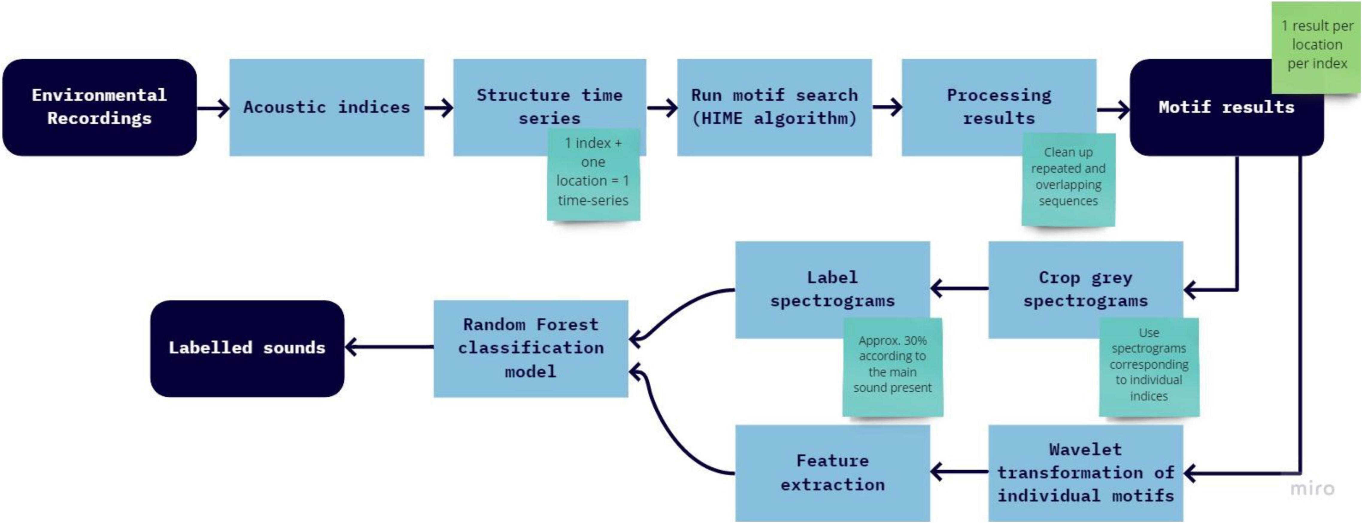
Figure 1. Flowchart with the analysis steps and expected results.
Subsequence Time-Series Search
The step-by-step process of the sub-sequence search is described in Table 1.
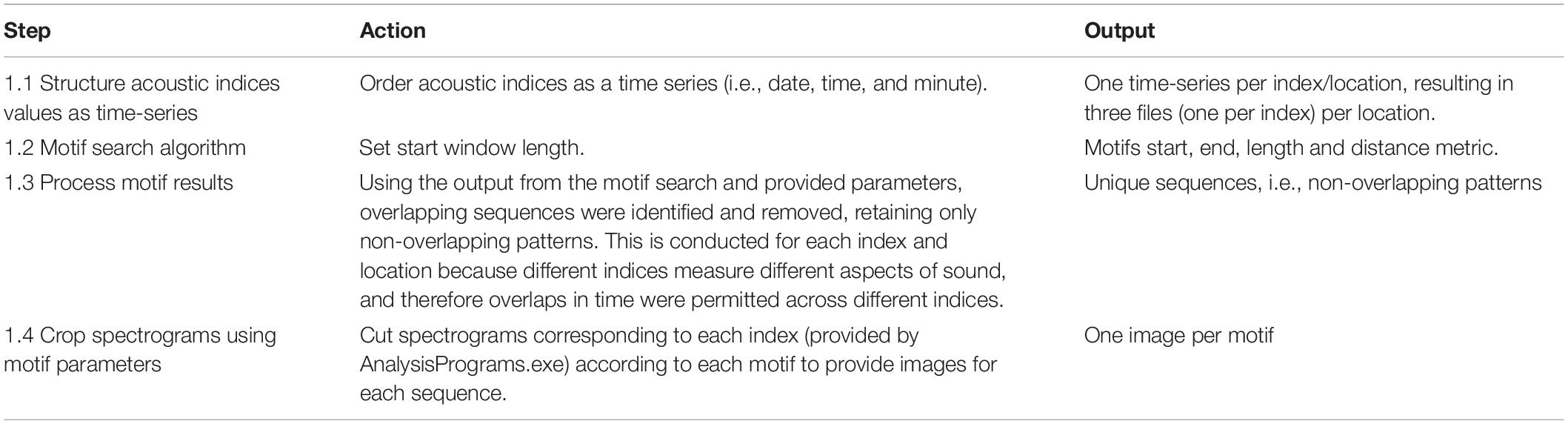
Table 1. Description of the steps to be followed to perform subsequence motif search, actions that should be done by the user and expected output.
Feature Extraction and Random Forest Model
Wavelet transform (Lau and Weng, 1995) and feature extraction were then performed on individual motifs (which are also time-series). Wavelets was used so both frequency and time information were preserved when extracting features. Each time-series was treated as an individual sample for feature extraction, training, and testing. Based on the extracted features, a Random Forest (RF) classification model was trained using manually labeled data and then the classification model was used to discriminate between sound categories within motifs, attributing ecological meaning to the motifs. RF classification is a supervised machine learning technique (Breiman, 2001), and has been used in numerous research fields such as genomics (Díaz-Uriarte and Alvarez de Andrés, 2006), satellite image classification (Pal, 2005), and soundscape analysis (Buxton et al., 2018). The algorithm classifies the data into groups using different combinations of features. It has been reported to perform well because it uses an ensemble learn strategy by combining different methods during the learning process, providing more accurate and generalized results (Cutler et al., 2012). In this study all the motifs were labeled. It was necessary to first test the testing sample size that maximized accuracy, while avoiding overfitting. This was done by progressively increasing training samples and measuring accuracy at each round. Accuracy was not greatly improved using more than 30% labeled data, and so this threshold was established. It was important that motifs were labeled using their corresponding spectrogram to show exactly what sound the index was capturing. In cases where the signal was unclear, these recordings were sound-truthed. This allowed maximizing label information, while keeping some generalization (i.e., not identifying species, for example). More categories of labels can increase training difficulty because categories become similar, making it difficult for the algorithm to discriminate between them. Additionally, biophony is now classified according to their soundtope (Farina, 2014). Soundtopes are the collective sounds produced by biophony at the same time.
Table 2 describes each step of the process and the expected output.

Table 2. Description of the steps to be followed to random forest classification, actions that should be done by the user and expected output.
Case Study
One of the limitations of using acoustic indices as a measure of biodiversity is that recent studies have shown variable success, that is largely context-dependent. In this case study, we demonstrate how our novel method overcomes this issue by testing and validating our approach in two very different ecosystems, including varying background noise and different acoustic recorders.
Dataset 1: Bowra
Data were collected at Bowra Wildlife Sanctuary in semi-arid western Queensland, Australia (Figures 2A,B). The sanctuary is owned by the Australian Wildlife Conservancy, and it is known for its abundant birdlife. The property covers more than 14,000 hectares in the Mulga Lands Bioregion of Australia (Figure 2B). The topography is mostly flat, and the vegetation is dominated by Acacia woodlands, Mitchell tussock grasslands, and Coolabah (Eucalyptus coolabah) woodlands along ephemeral creek lines. The region has very low annual precipitation rates, with an annual mean of 373.3 mm (Australian Government Bureau of Meteorology, 2020).
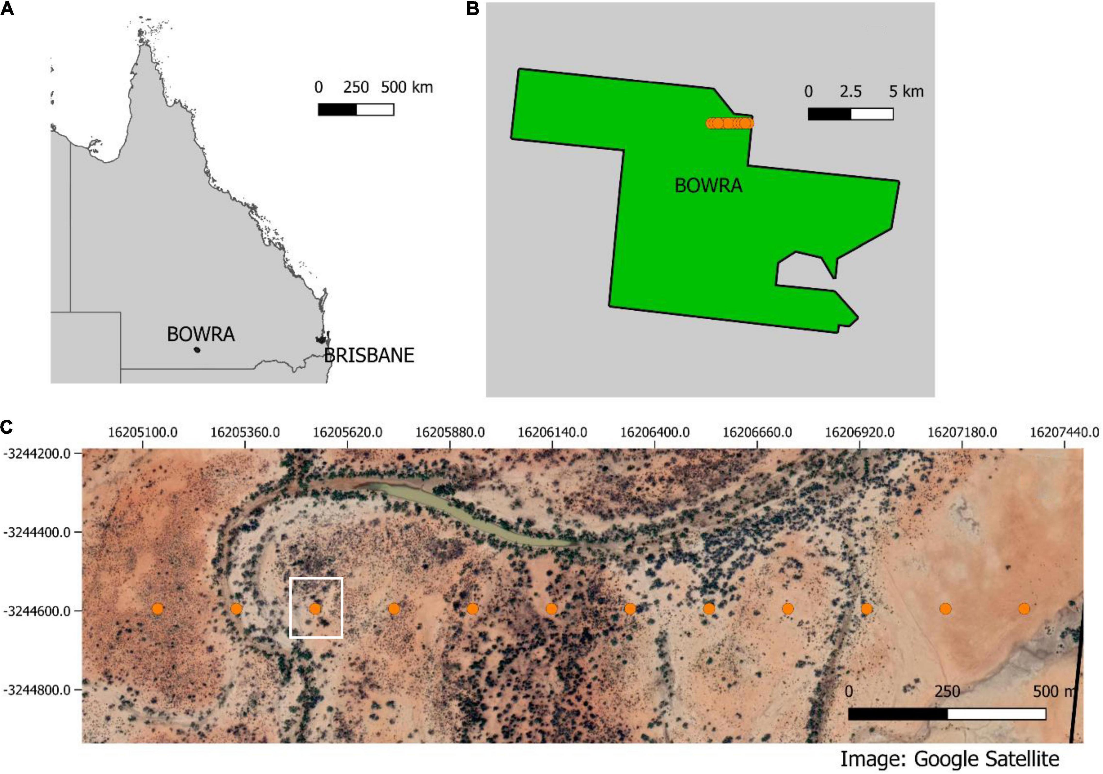
Figure 2. (A) Queensland map indicating Brisbane and Bowra. (B) shows in orange the transect inside the property and (C) show the transects and a Google satellite layer with the different vegetation communities across the transect. The white square highlights the point that will be used here as an example for figures.
Audio Sampling
Data were acquired using 12 SongMeter four recorders (Wildlife Acoustics), with a sampling rate of 44.1 kHz and 16 bits in stereo. Recorders were placed 200 m apart, (Figures 2B,C), operating continuously for approximately 40 h/sampling point. Sampling points were selected across a gradient of different vegetation communities and proximity to creek lines. To demonstrate the methods in a graphical way, one sampling point was chosen (white square in Figure 2C) for data visualization.
The data collection period coincided with a dust storm with high wind speeds, so recordings were very noisy and biophony was masked for large recording segments (pink/purple across all frequency bands in Figure 4A). While noise presents a challenge for data analysis, environmental conditions vary and are beyond researcher control, thus it is important that the method presented here is tested under varied and real circumstances.
Dataset 2: Samford Ecological Research Facility
The second dataset used was 1 month of data (March 2015) from the Samford Ecological Research Facility (SERF), a SuperSite in the Terrestrial Ecosystem Research Network (TERN). The TERN initiative established in 2009 monitors terrestrial ecosystem attributes over time at a continental scale. The data collected through this initiative are freely available through the TERN data portal1.
Samford Ecological Research Facility is situated approximately 20 km from Brisbane in the South-East Queensland Bioregion, Australia (Figure 3). The region experiences a sub-tropical climate and high levels of forest fragmentation and urbanization (Figure 3). The topography is gently undulating, and the vegetation consists of Eucalypt open forest (dominated by Eucalyptus tereticornis, Eucalyptus crebra and Corymbia species) and notophyll vine forest.
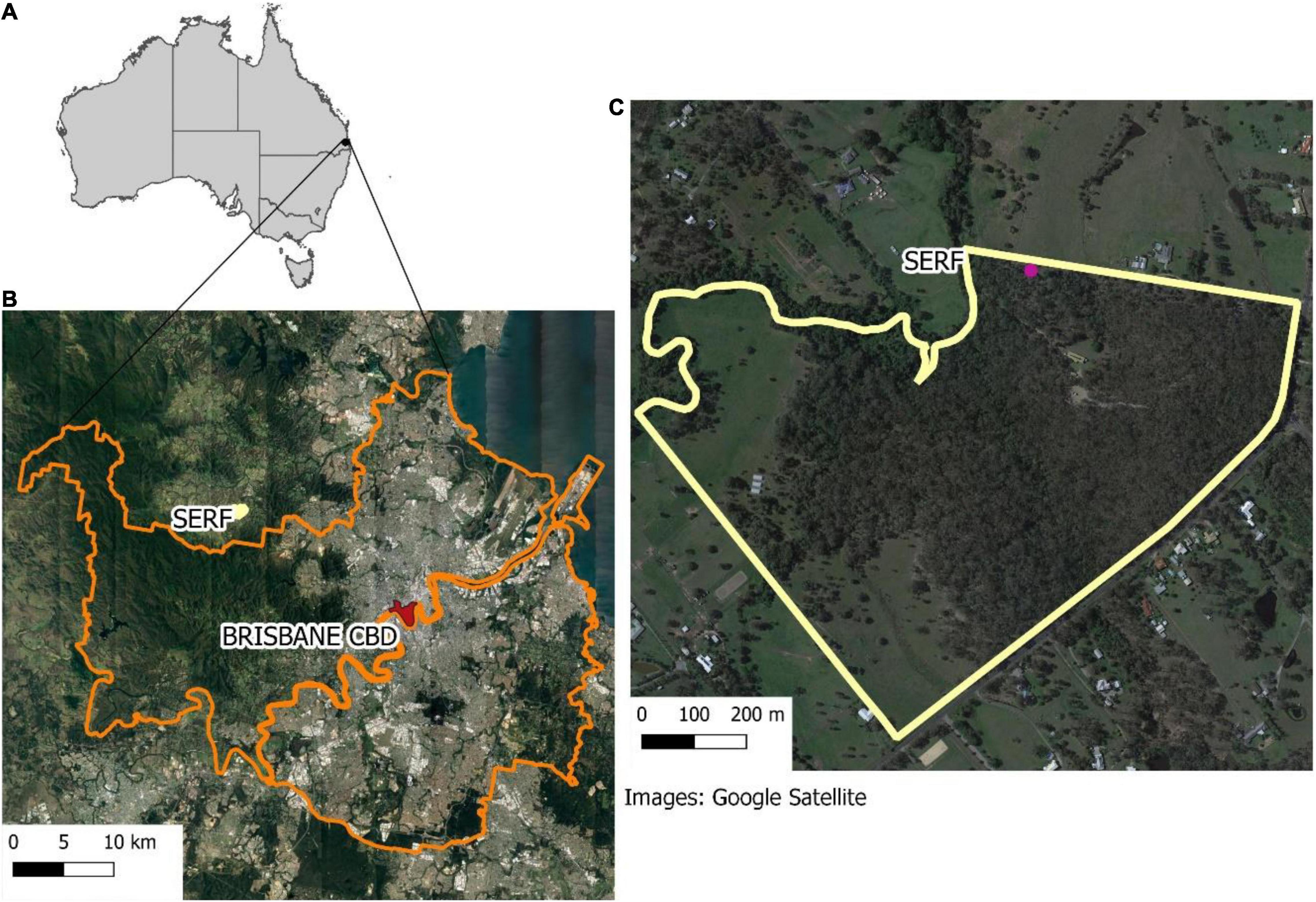
Figure 3. (A) Location map of Samford Ecological Research Facility (SERF) in Australia. (B) SERF in relation to Brisbane CBD and great Brisbane. (C) Shows the property and the pink dot corresponding to the sampling point.
Audio Sampling
The audio was collected continuously for 1 month using one SongMeter2 (Wildlife Acoustics) at 22,050 Hz, in WAV format. The sampling point was located on the edge of the property as demonstrated in Figure 3.
Results
Different lengths and minimum window sizes were tested for the two datasets and the minimum length selected was 30 min for both datasets. From an ecological perspective, 30 min of recording provides good resolution of fine-scale phenomena (e.g., a single species calling). Moreover, it can reveal soundscape changes throughout a day as the HIME progressively increases the window size. Having the same window length for both datasets is an advantage as it allows future comparisons to be made between results. All the selected motifs were labeled for both datasets so that the model accuracy could be measured, and sample size could be correctly estimated. The Bowra dataset had 549 selected motifs with a mean distance of 3.88 ± 1.24 and a mean length (in minutes) of 35.14 ± 3.88. The SERF dataset had 789 selected motifs with a mean distance of 4.28 ± 0.81 and a mean length (in minutes) of 36.02 ± 2.83. SERF dataset had 10% more hours than Bowra (542 and 494, respectively) and 43% more selected motifs.
Dataset 1: Bowra
Figures 4C,E,G show the motifs found (in color) for each index in relation to the whole time-series for one sampling point at Bowra. These figures reveal that for all three indices, the hours of the day that correspond to dawn (5:15–5:16 h) and dusk (6:49–6:50 h) most motifs were identified, while almost none in the middle of the day. It can also be seen on the gray-scale spectrograms how each index is capturing slightly different soundscape components, although all of them recorded wind in the middle of the day (blurred sections) (Figures 4B,D,F). It is also evident different motifs identified across indices (Figures 4C,E,G).
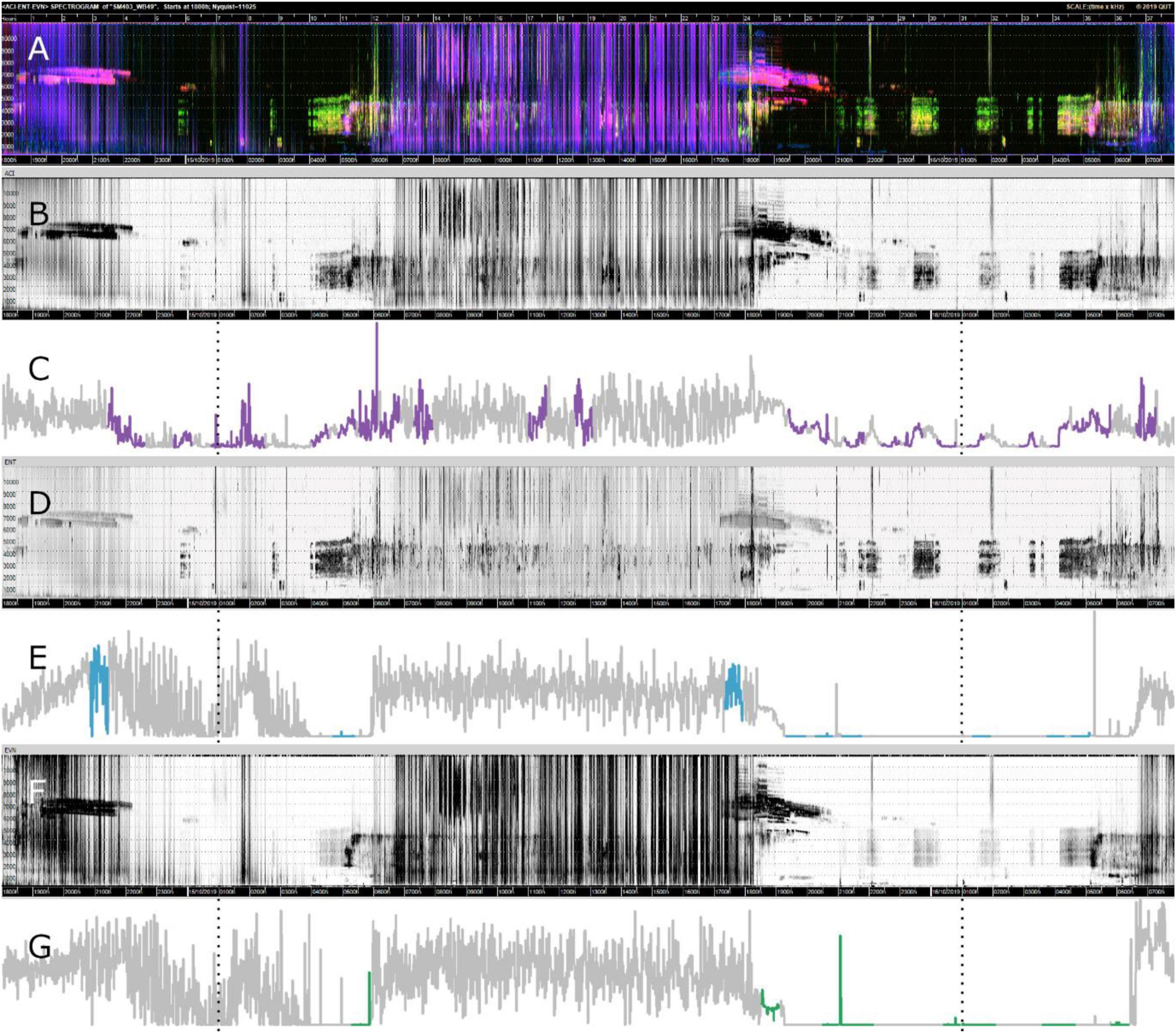
Figure 4. Visualizations of data from Bowra. The dotted lines are marking midnight. (A) False-color Spectrogram; (B) ACI gray-scale spectrogram; (C) ACI time-series and motifs (purple); (D) ENT gray-scale spectrogram; (E) ENT time-series with motifs (blue); (F) EVN gray-scale spectrogram; (G) EVN time-series with motifs (green).
Component Classification
The Component classification had an overall accuracy of 75%. The accuracy per category and overall misclassifications can be seen in Figure 5. The model correctly identified most biophony (94%) motifs while geophony motifs were less accurately identified (45%).
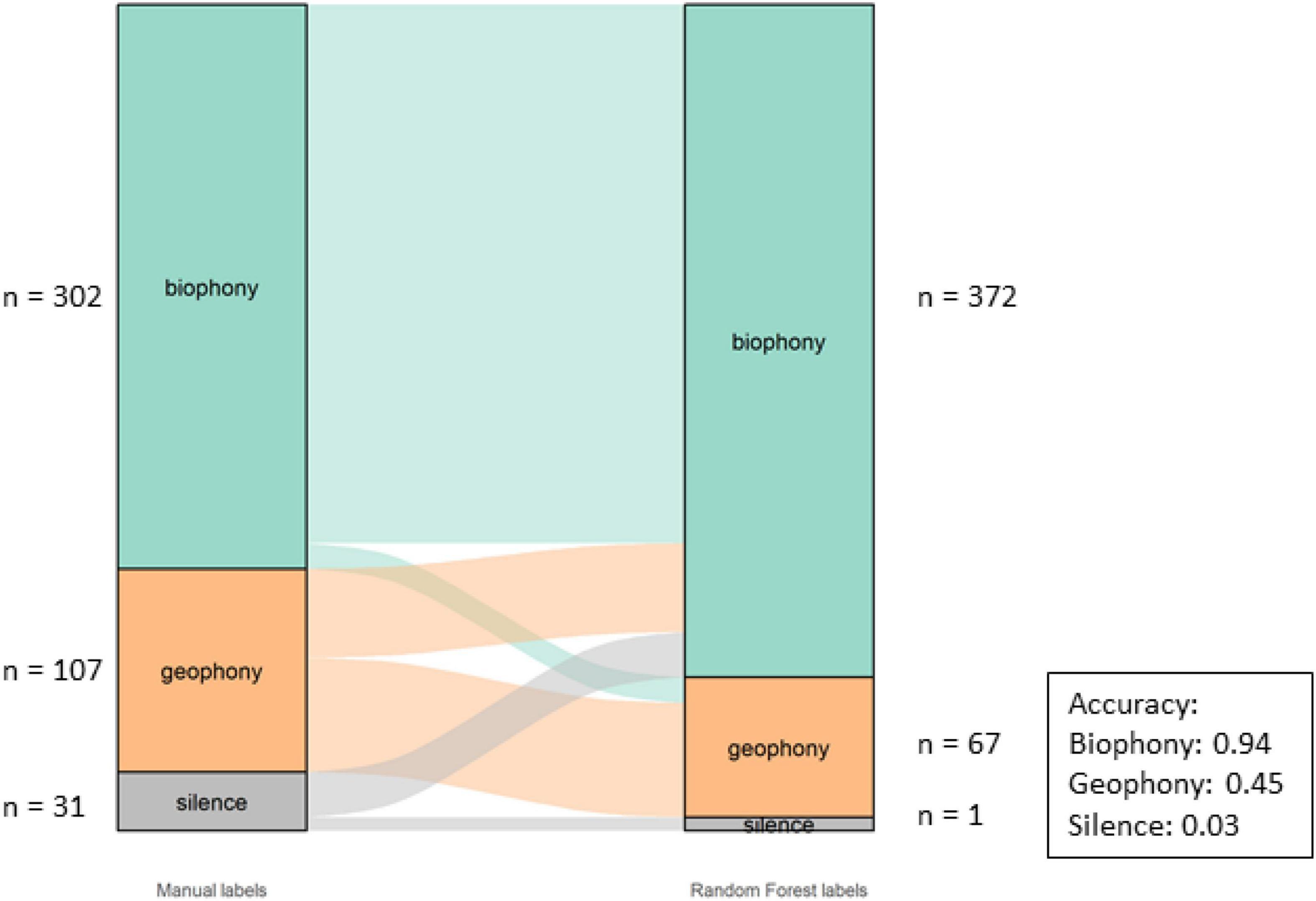
Figure 5. Alluvial graph showing proportions and number of motifs of manual labels on the left-hand and model labels on the right-hand side for the component in the Bowra dataset. The lines in the middle going from manual to model labels indicate the misclassification. The accuracy per class is also shown in the figure.
Class Classification
The overall accuracy of the Class labels was 70%. The model performed better for birds (80%) than insects (59%) for this dataset (Figure 6).
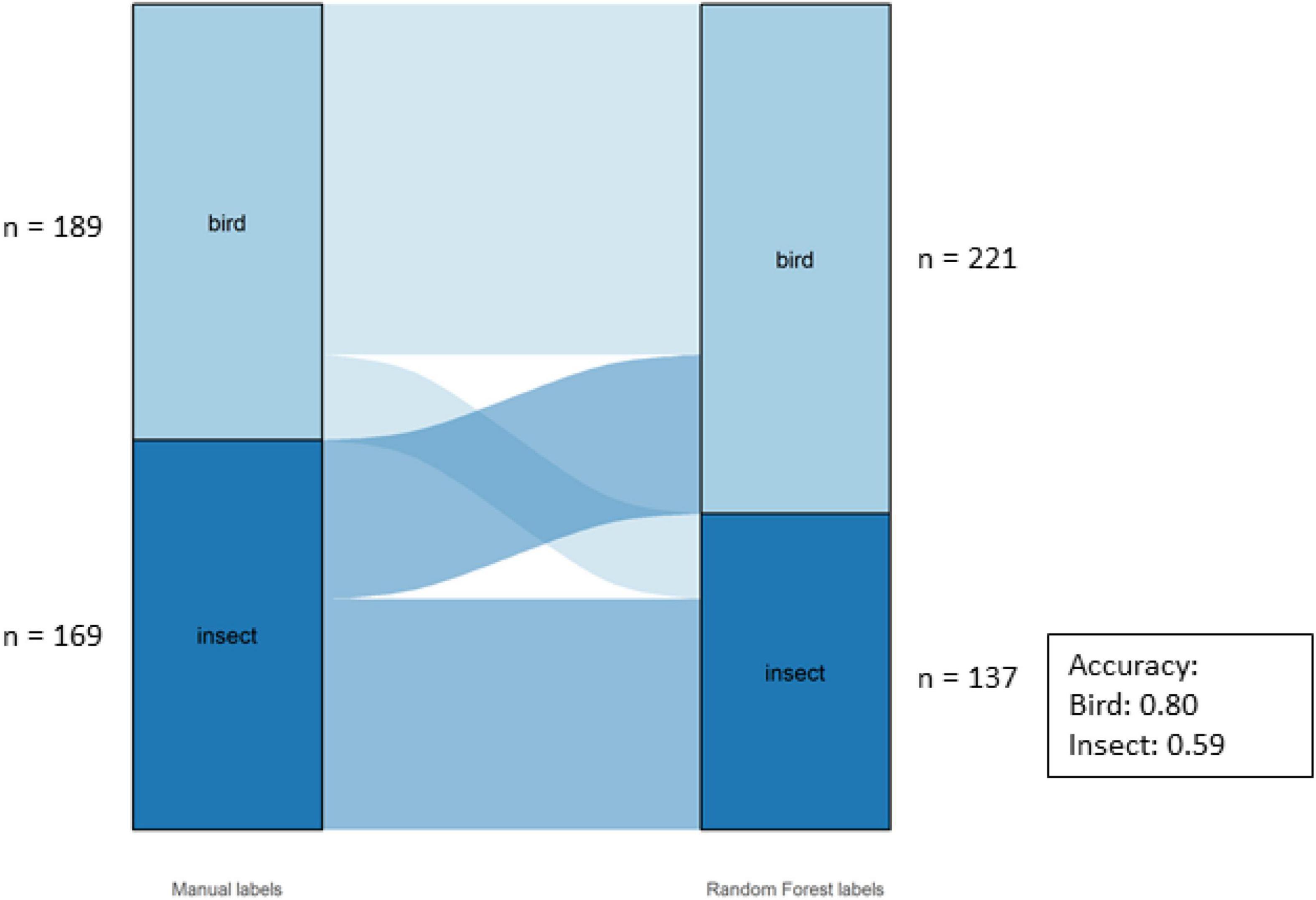
Figure 6. Alluvial graph showing proportions and number of motifs of manual labels on the left-hand and model labels on the right-hand side for the classes in the Bowra dataset. The lines in the middle going from manual to model labels indicate the misclassification. The accuracy per class is also shown in the figure.
Dataset 2: Samford Ecological Research Facility
Figures 7C,E,G shows 1 day of the complete time-series with the motifs identified in color. The false-color spectrogram can be seen in Figure 7A and the corresponding gray-scale spectrograms can be seen in Figures 7B,D,F. As seen for Bowra, some segments were interpreted as significant by the motif search algorithm, whereas others were not.
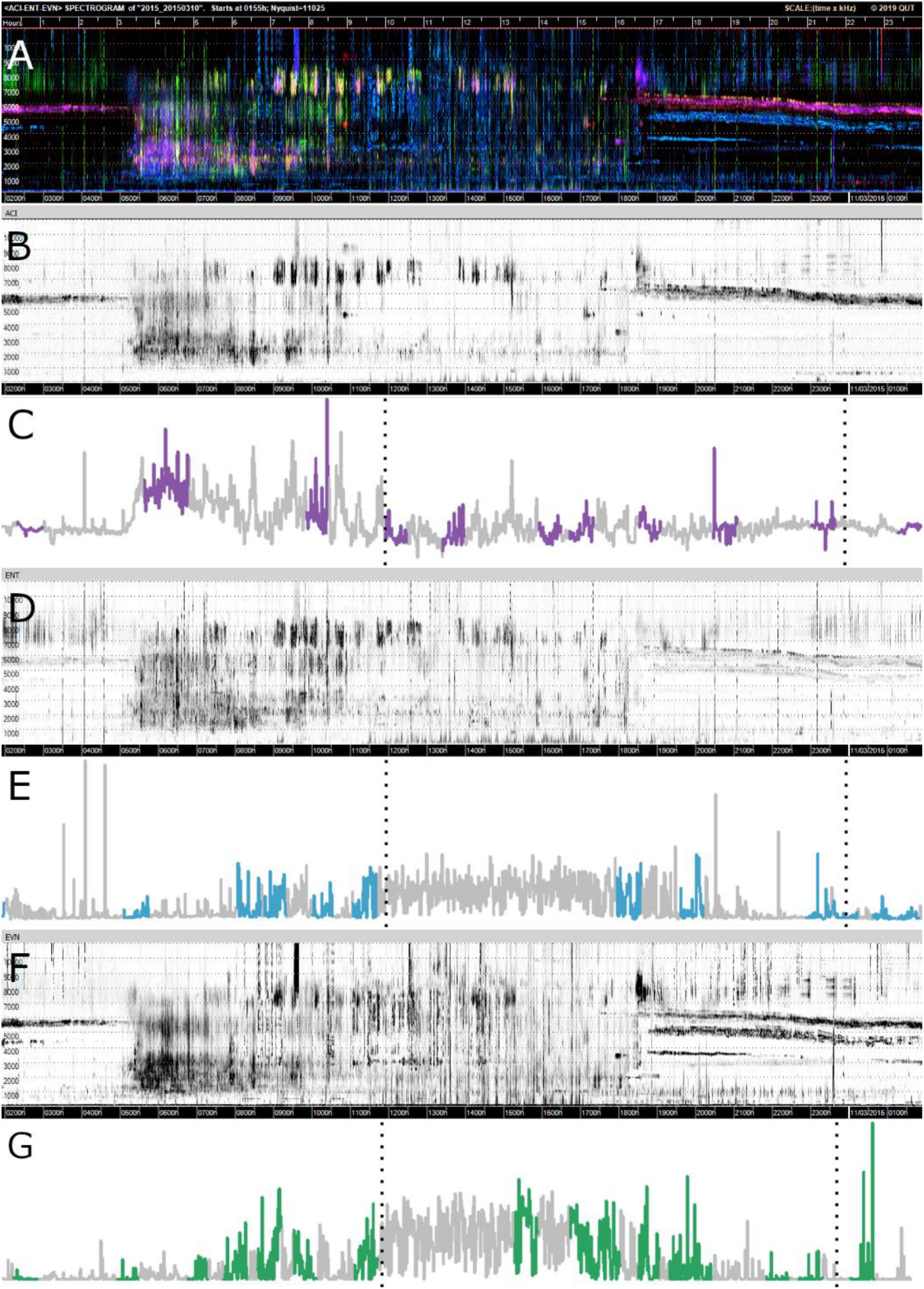
Figure 7. Visualizations of data from 1 day (10/03/2015) of SERF dataset. The dotted lines are marking midday and midnight as reference. (A) False-color Spectrogram; (B) ACI gray-scale spectrogram; (C) ACI time-series and motifs (purple); (D) ENT gray-scale spectrogram; (E) ENT time-series with motifs (blue); (F) EVN gray- scale spectrogram; (G) EVN time-series with motifs (green).
Component Classification
The overall accuracy of the model classification was 73% and the performance per Component can be seen in Figure 8. The model misclassified motifs primarily due to the presence of geophony alongside “dominant sounds” in the recordings. In these cases, the algorithm has identified segments as geophony, whereas the researcher has not.
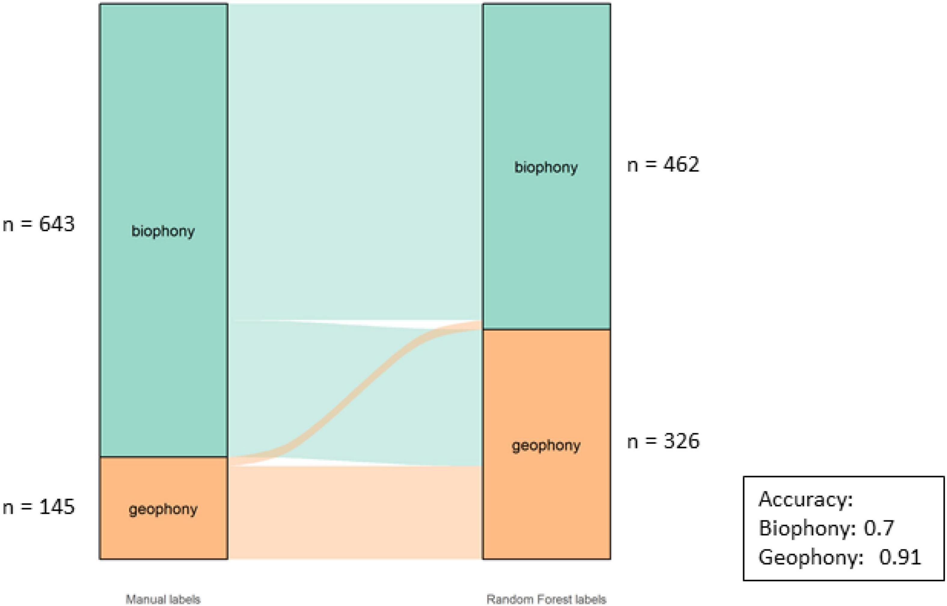
Figure 8. Alluvial graph showing proportions and number of motifs of manual labels on the left-hand and model labels on the right-hand side for the components in the SERF dataset. The lines in the middle going from manual to model labels indicate the misclassification. The accuracy per Class is also shown in the figure.
Class Classification
The overall accuracy for the Classes was 81%. The individual accuracies for the Classes can be seen in Figure 9. There were three classes for this dataset: birds, insects and “both,” as there were motifs with both insects and birds, especially during the dawn and dusk choruses.
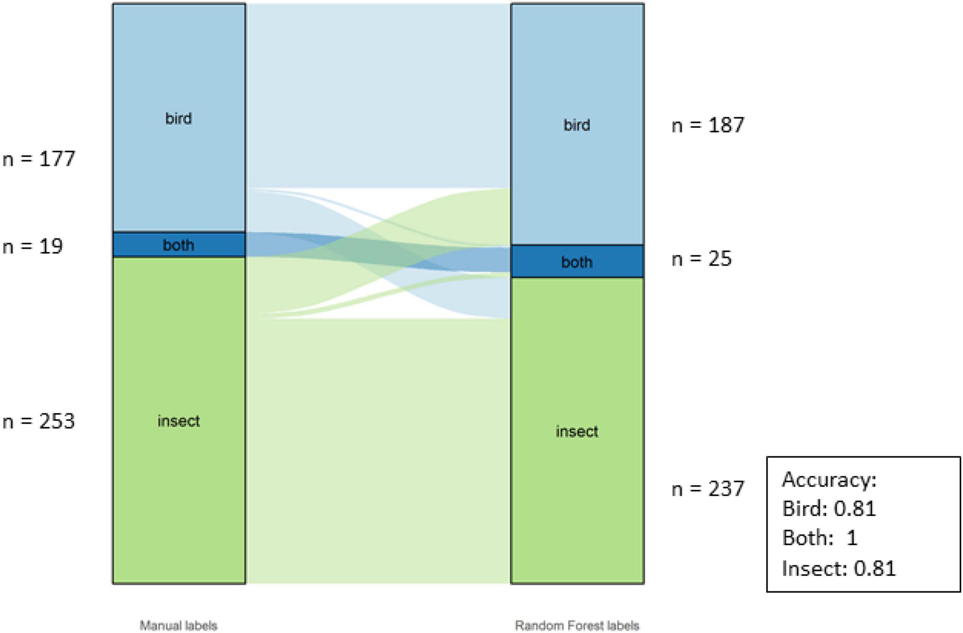
Figure 9. Alluvial graph showing proportions and number of motifs of manual labels on the left-hand and model labels on the right-hand side for the classes in the SERF dataset. The lines in the middle going from manual to model labels indicate the misclassification. The accuracy per Class is also shown in the figure.
Discussion
The approach proposed here using time-series motif discovery and random forest classification represents a significant improvement in how acoustic indices are currently analyzed for terrestrial soundscapes. It resolves some major challenges and constraints associated with acoustic data analysis including: (1) accounts for temporal autocorrelation of acoustic data, which violates most statistical test assumptions; (2) combines more than one index to assign soundscape components; and (3) performs in different contexts, as demonstrated by the finding that the same set of indices identified the same soundscape components in different ecosystems surveyed at different times, using varying recording schemes.
Acoustic recording and indices are now routinely used to monitor biodiversity (Doohan et al., 2019; Moreno-Gómez et al., 2019), but statistical analysis of recordings is problematic due to temporal autocorrelation. By using sub-sequence time-series search, we were able to group sequences of minutes with repetitive patterns across the recordings, reducing the number of consecutive minutes analyzed as independent samples.
Acoustic data analysis approaches are varied and include linear mixed models (Francomano et al., 2020), mean differences (Carruthers-Jones et al., 2019), manual inspection and tagging species or groups of interest (Ferreira et al., 2018) or using non-index based metrics (like amplitude and frequency) direct from sound files (Furumo and Aide, 2019). Despite the variety of ways to analyze sound data, single index approach is still one of the most common approaches. As previously stated, single index data can be problematic because they cannot be consistently interpreted across different taxonomic groups or environments. For example, studies using ACI have shown that this index was positively correlated with bird species (Jorge et al., 2018; Mitchell et al., 2020), but also rain and wind (Duarte et al., 2015). Acoustic entropy has been found to have higher values in biodiversity rich habitats (Sueur et al., 2008), although higher values in quiet recordings and lower values in recordings dominated by insects have also been documented (Bradfer-Lawrence et al., 2019). Other studies have also tried to find a direct relationship between one index and one taxonomic group (Brown et al., 2019; Indraswari et al., 2020) but this relationship often does not hold across environments. From these findings we can conclude that a single index provides only a crude or obscure representation of biodiversity and is context-dependant. However, in our study, we have developed, validated and tested a new workflow that can be used in different terrestrial environments. This is particularly important because with recent advances in development of cost-effective ecoacoustic technology, passive acoustic recording is becoming a commonplace ecological survey approach worldwide. It is important that analytical tools are developed to meet this need, and are transferable across environments, providing standardized outputs for comparison or benchmarking.
An alternative to analyzing single index data is to combine indices, but this has been rarely attempted. One study used clusters to combine indices and classify major soundscape components (Phillips et al., 2018). However, their method still relies on listening to many recording minutes, which is extremely time-consuming and usually not feasible for large datasets. Another study combined indices using RF models to predict avian species richness (Buxton et al., 2018) and revealed that acoustic entropy and ACI were among the best predictors of avian biodiversity. But still, their aim was to link indices to a specific taxonomic group. Our approach is different because it shifts the focus from the index itself, to instead examine what is being captured by it. While often the focus of an ecological study is a target species or taxonomic group, soundscapes can provide valuable insights on processes (such as geophony and anthropophony) that may influence biodiversity. Until now, no analytical approach exists that can efficiently extract soundscape components in a semi-supervised and transferable way.
Using index-based spectrograms for visual inspection of recordings, we were able to accurately assign sound labels to motifs, extrapolating these labels to the whole data. Although a certain level of generalization was required when using multiple indices and automated classification techniques, this approach represents a progression from single indices and the manual identification of sounds or calls. Along with the generalization required, there were also issues with misclassifications by the algorithm. Nevertheless, inspection of misclassified motifs showed that, for example, some of them that were not classified as wind, did have wind present. The labeling process was based on the most predominant sound, which does not exclude the possibility of having more than one sound present at a given motif. In fact, the presence of more than one soundscape component is quite common, and for the SERF data here presented an additional label had to be created to address multiple dominant sounds in one motif. Ecosystems are complex and biodiversity is subject to a variety of influencing factors that will change according to geography and its features (Gaston, 2000). This variation challenges the use of automatic analyses, and it also makes it harder to compare different contexts. Nevertheless, it is necessary to establish a baseline for analysis so recordings can be effectively used for environmental and temporal comparisons. Moreover, it highlights the importance of the label process that provides the researcher with the opportunity to adjust the method to the context.
As the two study sites were in different ecoregions (Bowra is classified under the Temperate Grasslands, Savannas and Shrublands while SERF is Temperate Broadleaf and Mixed Forest (Environment Australia, 2000), it was expected that their soundscapes would vary due to the distinct biodiversity, ecology, and environmental conditions. Besides expected differences, the SERF dataset had 10% more minutes than Bowra, but 43% more motifs. Potential explanations include that SERF has a more complex soundscape, or more likely that the increase may be attributed to the lack of wind at SERF relative to Bowra, resulting in more minutes with signal and less noise.
Although soundscapes are known to vary between different environments, major soundtopes (Farina, 2014) were still expected to be found in both ecosystems (e.g., dawn and dusk choruses). Daily cycles were evident across the month at SERF, although variation could still be detected. This reflects environmental processes which also vary naturally across days. For example, areas near urban settlements, such as SERF, traffic noise can exhibit differences between weekdays and weekends. Biophony is also expected to change in response to temperature, rainfall, sunlight, and many other environmental factors that influence animal behavior (Pijanowski et al., 2011). The differences found here among and within ecosystems emphasizes again the importance of labeling motifs by a researcher before running the algorithm. Each recording will have distinct features that need to be addressed before data analysis. Furthermore, it provides an opportunity for the researcher to understand patterns and to become acquainted with the data specific to the site. It is also important to keep in mind that like other sampling methods, acoustic surveys are a snapshot of the moment in which the recordings were made. In order to track changes and effectively use this method as a biodiversity monitoring tool, it is important to establish sampling schemes that can capture different moments in time so that natural variation can be examined (Metcalf et al., 2020), as well as man-made impacts.
The labels in this study were generalized, however, future research could attempt to create more specific categories. At the same time, we argue that keeping upper levels of categories is important for model optimization, but it also might be useful when comparing results across datasets and studies. For example, every environment might have different species assemblages but similar patterns of biophony. For this reason, we believe the method presented here will help standardize analyses in ecoacoustics research. Another improvement that can be done is to assign more than one soundscape category per motif, creating a rank of sound presence. In this way, the misclassifications could be measured more accurately and potentially improved.
Conclusion
Ecoacoustics is a promising tool which is widely used to monitor biodiversity, and it has increased even more with the advent of acoustic indices. Nevertheless, until now there has been no consensus on how to transform acoustic indices into broad, transferrable ecological information, especially when combining indices. It is crucial to have an approach that standardizes and enables rapid assessment of terrestrial soundscapes. Although the analysis presented here treats indices separately as independent time series, there is no distinction between them for classification. This is important because it addresses the narrow assumption that each index serves as a good proxy for measuring specific taxonomic groups, and that these relationships will hold in different contexts. By combining different analysis techniques (time-series motif discovery and RF model classification), we were able to label grouped minutes of recordings translating acoustic indices into important components of the soundscape. We tested this approach on two datasets acquired using different recording devices and from different environments, providing strong evidence that this method can capture important temporal patterns in insect and bird biodiversity, as well as environmental geophonic sounds across environments. Given the global biodiversity loss that we are currently facing in the Anthropocene (Johnson et al., 2017), it is even more important that monitoring and methods of analysis are developed allowing to track changes in biodiversity.
Data Availability Statement
The datasets presented in this study can be found in online repositories. The names of the repository/repositories and accession number(s) can be found below: https://doi.org/10.5281/zenodo.4784758.
Author Contributions
MS, SF, and BL conceived the ideas. MS and DT collected the data. MS and BL designed the methodology and analyzed the data. All authors contributed to data interpretation, drafts, critical revision and gave final approval for submission.
Conflict of Interest
The authors declare that the research was conducted in the absence of any commercial or financial relationships that could be construed as a potential conflict of interest.
Publisher’s Note
All claims expressed in this article are solely those of the authors and do not necessarily represent those of their affiliated organizations, or those of the publisher, the editors and the reviewers. Any product that may be evaluated in this article, or claim that may be made by its manufacturer, is not guaranteed or endorsed by the publisher.
Acknowledgments
MS acknowledges QUT for funding; AWC for access to the sanctuary and Brendan Doohan for assistance with fieldwork.
Footnotes
References
Aide, T. M., Hernández-Serna, A., Campos-Cerqueira, M., Acevedo-Charry, O., and Deichmann, J. L. (2017). Species richness (of insects) drives the use of acoustic space in the tropics. Remote Sens. 9:1096. doi: 10.3390/rs9111096
Aldrich, E. (2020). Wavelets: Functions for Computing Wavelet Filters, Wavelet Transforms and Multiresolution Analyses. Available online at: https://cran.r-project.org/package=wavelets. (accessed Feb 17, 2020).
Australian Government Bureau of Meteorology (2020). Graphical Climate Statistics for Australian Locations. Available online at: http://www.bom.gov.au/jsp/ncc/cdio/cvg/av?p_stn_num=044026&p_prim_element_index=18&p_display_type=statGraph&period_of_avg=ALL&normals_years=allYearOfData&staticPage= (accessed April 20, 2020).
Bonthoux, S., Lefèvre, S., Herrault, P.-A., and Sheeren, D. (2018). Spatial and temporal dependency of NDVI satellite imagery in predicting bird diversity over france. Remote Sens. 10:1136. doi: 10.3390/rs10071136
Bradfer-Lawrence, T., Bunnefeld, N., Gardner, N., Willis, S. G., and Dent, D. H. (2020). Rapid assessment of avian species richness and abundance using acoustic indices. Ecol. Indic. 115:106400. doi: 10.1016/j.ecolind.2020.106400
Bradfer-Lawrence, T., Gardner, N., Bunnefeld, L., Bunnefeld, N., Willis, S. G., and Dent, D. H. (2019). Guidelines for the use of acoustic indices in environmental research. Methods. Ecol. Evol. 10, 1796–1807. doi: 10.1111/2041-210x.13254
Brodie, S., Allen-Ankins, S., Towsey, M., Roe, P., and Schwarzkopf, L. (2020). Automated species identification of frog choruses in environmental recordings using acoustic indices. Ecol. Indic. 119:106852. doi: 10.1016/j.ecolind.2020.106852
Brown, A., Garg, S., and Montgomery, J. (2019). Automatic rain and cicada chorus filtering of bird acoustic data. Appl. Soft Comput. J. 81:105501. doi: 10.1016/j.asoc.2019.105501
Buxton, R. T., Agnihotri, S., Robin, V. V., Goel, A., and Balakrishnan, R. (2018). Acoustic indices as rapid indicators of avian diversity in different land-use types in an Indian biodiversity hotspot. J. Ecoacoustics 2:8. doi: 10.22261/jea.gwpzvd
Cardinale, B. J., Duffy, J. E., Gonzalez, A., Hooper, D. U., Perrings, C., Venail, P., et al. (2012). Biodiversity loss and its impact on humanity. Nature 486, 59–67. doi: 10.1038/nature11148
Carruthers-Jones, J., Eldridge, A., Guyot, P., Hassall, C., and Holmes, G. (2019). The call of the wild: investigating the potential for ecoacoustic methods in mapping wilderness areas. Sci. Total Environ. 695:133797. doi: 10.1016/j.scitotenv.2019.133797
Cutler, A., Cutler, D. R., and Stevens, J. R. (2012). “Random forests,” in Ensemble Machine Learning, eds C. Zhang and Y. Ma (Boston, MA: Springer US), 157–175. doi: 10.1007/978-1-4419-9326-7_5
Díaz-Uriarte, R., and Alvarez de Andrés, S. (2006). Gene selection and classification of microarray data using random forest. BMC Bioinformatics 7:3. doi: 10.1186/1471-2105-7-3
Doohan, B., Fuller, S., Parsons, S., and Peterson, E. E. (2019). The sound of management: acoustic monitoring for agricultural industries. Ecol. Indic. 96, 739–746. doi: 10.1016/j.ecolind.2018.09.029
Duarte, M. H. L., Sousa-Lima, R. S. S., Young, R. J., Vasconcelos, M. F., Bittencourt, E., Scarpelli, M. D. A., et al. (2021). Changes on soundscapes reveal impacts of wildfires in the fauna of a Brazilian savanna. Sci. Total Environ. 769:144988. doi: 10.1016/j.scitotenv.2021.144988
Duarte, M. H. L., Sousa-Lima, R. S., Young, R. J., Farina, A., Vasconcelos, M., Rodrigues, M., et al. (2015). The impact of noise from open-cast mining on Atlantic forest biophony. Biol. Conserv. 191, 623–631. doi: 10.1016/j.biocon.2015.08.006
Environment Australia (2000). Revision of the Interim Biogeographic Regionalisation for Australia (IBRA) and Development of Version 5.1 Summary Report. Available online at: http://www.environment.gov.au/system/files/resources/401ff882-fc13-49cd-81fe-bc127d16ced1/files/revision-ibra-development-5-1-summary-report.pdf (accessed Nov 20, 2001).
Farina, A. (2014). Soundscape Ecology: Principles, Patterns, Methods and Applications. Dordrecht: Springer Science+Business Media, doi: 10.1007/978-94-007-7374-5
Ferreira, L. M., Oliveira, E. G., Lopes, L. C., Brito, M. R., Baumgarten, J., Rodrigues, F. H., et al. (2018). What do insects, anurans, birds, and mammals have to say about soundscape indices in a tropical savanna. J. Ecoacoustics 2:VH6YZ. doi: 10.22261/JEA.PVH6YZ
Fontúrbel, F. E., Orellana, J. I., Rodríguez-Gómez, G. B., Tabilo, C. A., and Castaño-Villa, G. J. (2021). Habitat disturbance can alter forest understory bird activity patterns: a regional-scale assessment with camera-traps. For. Ecol. Manage. 479:118618. doi: 10.1016/j.foreco.2020.118618
Francomano, D., Gottesman, B. L., and Pijanowski, B. C. (2020). Biogeographical and analytical implications of temporal variability in geographically diverse soundscapes. Ecol. Indic. 112:105845. doi: 10.1016/j.ecolind.2019.105845
Froidevaux, J. S. P., Zellweger, F., Bollmann, K., and Obrist, M. K. (2014). Optimizing passive acoustic sampling of bats in forests. Ecol. Evol. 4, 4690–4700. doi: 10.1002/ece3.1296
Furumo, P. R., and Aide, M. T. (2019). Using soundscapes to assess biodiversity in Neotropical oil palm landscapes. Landsc. Ecol. 34, 911–923. doi: 10.1007/s10980-019-00815-w
Gage, S. H., and Axel, A. C. (2014). Visualization of temporal change in soundscape power of a Michigan lake habitat over a 4-year period. Ecol. Inform. 21, 100–109. doi: 10.1016/j.ecoinf.2013.11.004
Gan, H., Zhang, J., Towsey, M., Truskinger, A., Stark, D., van Rensburg, B. J., et al. (2020). Data selection in frog chorusing recognition with acoustic indices. Ecol. Inform. 60:101160. doi: 10.1016/j.ecoinf.2020.101160
Gao, Y., and Lin, J. (2017). “Efficient discovery of time series motifs with large length range in million scale time series,” in Proceedings of the IEEE International Conference on Data Mining (ICDM) 2017-Novem, New Orleans, LA, 1213–1222. doi: 10.1109/ICDM.2017.8356939
Genuer, R., and Poggi, J. M. Tuleau-Malot, C. (2010). Variable selection using random forests. Pattern Recognit. Lett. 31, 2225–2236. doi: 10.1016/j.patrec.2010.03.014
Gibb, R., Browning, E., Glover-Kapfer, P., and Jones, K. E. (2019). Emerging opportunities and challenges for passive acoustics in ecological assessment and monitoring. Methods Ecol. Evol. 10, 169–185. doi: 10.1111/2041-210X.13101
Hayashi, K., Erwinsyah, Lelyana, V. D., and Yamamura, K. (2020). Acoustic dissimilarities between an oil palm plantation and surrounding forests: analysis of index time series for beta-diversity in South Sumatra, Indonesia. Ecol. Indic. 112:106086. doi: 10.1016/j.ecolind.2020.106086
Indraswari, K., Bower, D. S., Tucker, D., Schwarzkopf, L., Towsey, M., and Roe, P. (2020). Assessing the value of acoustic indices to distinguish species and quantify activity: a case study using frogs. Freshw. Biol. 65, 142–152. doi: 10.1111/fwb.13222
Johnson, C. N., Balmford, A., Brook, B. W., Buettel, J. C., Galetti, M., Guangchun, L., et al. (2017). Biodiversity losses and conservation responses in the Anthropocene. Science 356, 270–275. doi: 10.1126/science.aam9317
Joppa, L. N., O’Connor, B., Visconti, P., Smith, C., Geldmann, J., Hoffmann, M., et al. (2016). Filling in biodiversity threat gaps. Science 352, 416–418. doi: 10.1126/science.aaf3565
Jorge, F. C., Machado, C. G., da Cunha Nogueira, S. S., and Nogueira-Filho, S. L. G. (2018). The effectiveness of acoustic indices for forest monitoring in Atlantic rainforest fragments. Ecol. Indic. 91, 71–76. doi: 10.1016/j.ecolind.2018.04.001
Kerr, J. T., and Ostrovsky, M. (2003). From space to species: ecological applications for remote sensing. Trends Ecol. Evol. 18, 299–305. doi: 10.1016/S0169-5347(03)00071-5
Krause, B., and Farina, A. (2016). Using ecoacoustic methods to survey the impacts of climate change on biodiversity. Biol. Conserv. 195, 245–254. doi: 10.1016/j.biocon.2016.01.013
Lau, K. M., and Weng, H. (1995). Climate signal detection using wavelet transform: how to make a time series sing. Bull. - Am. Meteorol. Soc. 76, 2391–2402.
Liu, B., Li, J., Chen, C., Tan, W., Chen, Q., and Zhou, M. (2015). Efficient motif discovery for large-scale time series in healthcare. IEEE Trans. Ind. Informatics 11, 583–590. doi: 10.1109/TII.2015.2411226
Machado, R. B., Aguiar, L., and Jones, G. (2017). Do acoustic indices reflect the characteristics of bird communities in the savannas of Central Brazil? Landsc. Urban Plan. 162, 36–43. doi: 10.1016/j.landurbplan.2017.01.014
McGovern, A., Rosendahl, D. H., Brown, R. A., and Droegemeier, K. K. (2011). Identifying predictive multi-dimensional time series motifs: an application to severe weather prediction. Data Min. Knowl. Discov. 22, 232–258. doi: 10.1007/s10618-010-0193-7
Metcalf, O. C., Barlow, J., Devenish, C., Marsden, S., Berenguer, E., and Lees, A. C. (2020). Acoustic indices perform better when applied at ecologically meaningful time and frequency scales. Methods Ecol. Evol. 2020, 421–431. doi: 10.1111/2041-210x.13521
Mitchell, S. L., Bicknell, J. E., Edwards, D. P., Deere, N. J., Bernard, H., Davies, Z. G., et al. (2020). Spatial replication and habitat context matters for assessments of tropical biodiversity using acoustic indices. Ecol. Indic. 119:106717. doi: 10.1016/j.ecolind.2020.106717
Moreno-Gómez, F. N., Bartheld, J., Silva-Escobar, A. A., Briones, R., Márquez, R., and Penna, M. (2019). Evaluating acoustic indices in the Valdivian rainforest, a biodiversity hotspot in South America. Ecol. Indic. 103, 1–8. doi: 10.1016/j.ecolind.2019.03.024
Nowak, M. M., Dziób, K., and Bogawski, P. (2019). Unmanned Aerial Vehicles (UAVs) in environmental biology: a review. Eur. J. Ecol. 4, 56–74. doi: 10.2478/eje-2018-0012
Pal, M. (2005). Random forest classifier for remote sensing classification. Int. J. Remote Sens. 26, 217–222. doi: 10.1080/01431160412331269698
Petrusková, T., Pišvejcová, I., Kinštová, A., Brinke, T., and Petrusek, A. (2016). Repertoire-based individual acoustic monitoring of a migratory passerine bird with complex song as an efficient tool for tracking territorial dynamics and annual return rates. Methods Ecol. Evol. 7, 274–284. doi: 10.1111/2041-210X.12496
Phillips, Y. F., Towsey, M., and Roe, P. (2018). Revealing the ecological content of long-duration audio-recordings of the environment through clustering and visualisation. PLoS One 13:e0193345. doi: 10.1371/journal.pone.0193345
Pieretti, N., Farina, A., and Morri, D. (2011). A new methodology to infer the singing activity of an avian community: the acoustic complexity index (ACI). Ecol. Indic. 11, 868–873. doi: 10.1016/j.ecolind.2010.11.005
Pijanowski, B. C., Villanueva-Rivera, L. J., Dumyahn, S. L., Farina, A., Krause, B. L., Napoletano, B. M., et al. (2011). Soundscape ecology: the science of sound in the landscape. Bioscience 61, 203–216. doi: 10.1525/bio.2011.61.3.6
Roe, P., Eichinski, P., Fuller, R. A., McDonald, P. G., Schwarzkopf, L., Towsey, M., et al. (2021). The Australian acoustic observatory. Methods Ecol. Evol. 2021, 1–7. doi: 10.1111/2041-210X.13660
Sánchez-Giraldo, C., Bedoya, C. L., Morán-Vásquez, R. A., Isaza, C. V., and Daza, J. M. (2020). Ecoacoustics in the rain: understanding acoustic indices under the most common geophonic source in tropical rainforests. Remote Sens. Ecol. Conserv. 6, 248–261. doi: 10.1002/rse2.162
Shannon, C. E., and Weaver, W. (1964). The Mathematical Theory of Communication. Urbana: University of Illinois Press, doi: 10.1109/TMAG.1987.1065451
Stafford, C. A., and Walker, G. P. (2009). Characterization and correlation of DC electrical penetration graph waveforms with feeding behavior of beet leafhopper, Circulifer tenellus. Entomol. Exp. Appl. 130, 113–129. doi: 10.1111/j.1570-7458.2008.00812.x
Sueur, J., Farina, A., Gasc, A., Pieretti, N., and Pavoine, S. (2014). Acoustic indices for biodiversity assessment and landscape investigation. ACTA Acust. United With Acust. 100, 772–781. doi: 10.3813/AAA.918757
Sueur, J., Pavoine, S., Hamerlynck, O., and Duvail, S. (2008). Rapid acoustic survey for biodiversity appraisal. PLoS One 3:e4065. doi: 10.1371/journal.pone.0004065
Towsey, M. (2018). The Calculation of Acoustic Indices Derived from Long-Duration Recordings of the Natural Environment. Brisbane, QLD: QUT ePrints.
Towsey, M., Truskinger, A., Cottman-Fields, M., and Roe, P. (2020). QutEcoacoustics/Audio-Analysis: Ecoacoustics Audio Analysis Software v20.11.2.0. doi: 10.5281/ZENODO.4274299
Towsey, M., Zhang, L., Cottman-Fields, M., Wimmer, J., Zhang, J., and Roe, P. (2014). Visualization of long-duration acoustic recordings of the environment. Proc. Comput. Sci. 29, 703–712. doi: 10.1016/j.procs.2014.05.063
Towsey, M., Znidersic, E., Broken-Brow, J., Indraswari, K., Watson, D. M., Phillips, Y., et al. (2018). Long-duration, false-colour spectrograms for detecting species in large audio data-sets. J. Ecoacoustics 2:6. doi: 10.22261/JEA.IUSWUI
Tucker, D., Gage, S. H., Williamson, I., and Fuller, S. (2014). Linking ecological condition and the soundscape in fragmented Australian forests. Landsc. Ecol. 29, 745–758. doi: 10.1007/s10980-014-0015-1
Ulloa, J. S., Aubin, T., Llusia, D., Bouveyron, C., and Sueur, J. (2018). Estimating animal acoustic diversity in tropical environments using unsupervised multiresolution analysis. Ecol. Indic. 90, 346–355. doi: 10.1016/j.ecolind.2018.03.026
Ulloa, J. S., Aubin, T., Llusia, D., Courtois, ÉA., Fouquet, A., Gaucher, P., et al. (2019). Explosive breeding in tropical anurans: environmental triggers, community composition and acoustic structure. BMC Ecol. 19:28. doi: 10.1186/s12898-019-0243-y
Villanueva-Rivera, L. J., Pijanowski, B. C., Doucette, J., and Pekin, B. (2011). A primer of acoustic analysis for landscape ecologists. Landsc. Ecol. 26, 1233–1246. doi: 10.1007/s10980-011-9636-9
Wrege, P. H., Rowland, E. D., Keen, S., and Shiu, Y. (2017). Acoustic monitoring for conservation in tropical forests: examples from forest elephants. Methods Ecol. Evol. 8, 1292–1301. doi: 10.1111/2041-210X.12730
Znidersic, E., Towsey, M., Roy, W. K., Darling, S. E., Truskinger, A., Roe, P., et al. (2020). Using visualization and machine learning methods to monitor low detectability species—The least bittern as a case study. Ecol. Inform. 55:101014. doi: 10.1016/j.ecoinf.2019.101014
Keywords: acoustic complexity index, acoustic ecology, acoustic indices, ecoacoustics, terrestrial soundscapes
Citation: Scarpelli MDA, Liquet B, Tucker D, Fuller S and Roe P (2021) Multi-Index Ecoacoustics Analysis for Terrestrial Soundscapes: A New Semi-Automated Approach Using Time-Series Motif Discovery and Random Forest Classification. Front. Ecol. Evol. 9:738537. doi: 10.3389/fevo.2021.738537
Received: 09 July 2021; Accepted: 23 November 2021;
Published: 17 December 2021.
Edited by:
Alexei B. Ryabov, University of Oldenburg, GermanyReviewed by:
Eugene B. Postnikov, Kursk State University, RussiaAileen Van Der Mescht, University of the Free State, South Africa
Copyright © 2021 Scarpelli, Liquet, Tucker, Fuller and Roe. This is an open-access article distributed under the terms of the Creative Commons Attribution License (CC BY). The use, distribution or reproduction in other forums is permitted, provided the original author(s) and the copyright owner(s) are credited and that the original publication in this journal is cited, in accordance with accepted academic practice. No use, distribution or reproduction is permitted which does not comply with these terms.
*Correspondence: Marina D. A. Scarpelli, bmluYXNjYXJwZWxsaUBnbWFpbC5jb20=