Space and Species Interactions in Welfare Estimates for Invasive Species Policy

Aquatic invasive species (AIS) can cause catastrophic damages to lake ecosystems. Bigheaded carp are one such species that pose a current threat to Lake Michigan. Bigheaded carp are expected to have spatially differentiated impacts on other aquatic species in the metapopulation. Policymakers must decide how much to invest in mitigation or conservation policies, if at all, by understanding how invasions impact social welfare or social wellbeing. Estimates of social welfare implications, however, may be biased if important interactions between species and space are overly simplified or aggregated out of the model. In this analysis, a bioeconomic model that links an ecological model with an economic model of recreational fishing behavior is used to complete a comparative analysis of the social welfare implications across several different ecological specifications to demonstrate what biases exist if species interactions are neglected or if ecological characteristics are assumed to be homogenous across space. Results of the bigheaded carp case study suggest that social welfare losses from the invasion vary substantially if species interactions are excluded and vary less if space is treated homogeneously.

Introduction

Lake-level invasions of non-indigenous aquatic invasive species (AIS) can disrupt lake ecosystems and lead to catastrophic damages. When presented with the possibility of such an issue, policymakers must first determine whether to invest in strategies to conserve or protect the metapopulations within the ecosystem and then they must decide how much to invest. Historically, policymakers and managers have relied on economic studies to help them allocate scarce funds to invasive species management and, thereby, conservation (e.g., Pimentel et al., 2000, 2005). The investment decisions are often influenced by estimates of economic damages or social welfare implications associated with the invasion that can be used in a benefit-cost analysis (Leung et al., 2002; Finnoff et al., 2005, 2010; Hanley and Roberts, 2019). Yet the usefulness of damage assessments or social welfare estimates can fall short and lead to poor investment decisions if the complex relationships between humans and species across space are overly simplified (see reviews of Perrings et al., 2000; Finnoff et al., 2010; Simberloff et al., 2013; Epanchin-Niell, 2017; Warziniack et al., 2021).

To better understand the consequences of oversimplification of complex relationships in assessments of economic costs, the study herein considers the potential invasion of an AIS in Lake Michigan. Silver Carp, Hypophthalmichthys molitrix, and Bighead Carp, Hypophthalmichthys nobilis, (collectively and henceforth bigheaded¹ carp) are AIS that have been traveling up the Mississippi River and are expected to enter the southern basin of Lake Michigan and spread throughout the lake. Currently, the invasion front is just 76 km away from Lake Michigan (Rutherford et al., 2021). The invasive bigheaded carp are strong competitors that may outcompete larval fish for algae and zooplankton (Solomon et al., 2016; Pendleton et al., 2017; Phelps et al., 2017; DeBoer et al., 2018) or may outcompete forage fish (e.g., alewife, Alosa pseudoharengus or rainbow smelt, Osmerus mordax) – which are primary food for the salmonines (e.g., Chinook salmon, Oncorhynchus tshawytscha, Coho salmon, Oncorhynchus kisutch, lake trout Salvelinus namaycush, or steelhead (rainbow trout), Oncorhynchus mykiss) that are economically important to the recreational sportfishing industry. Young bigheaded carp can be a food source for piscivores that are also important to the sportfishing industry (Wittmann et al., 2015; Anderson, 2016), although rapid growth in body size of juvenile bigheaded carp may limit their positive effects on piscivores predation (Kolar et al., 2007). Further, there is concern that bigheaded carp may disrupt the energy flow from primary producers to fishery species and make the fishery unsustainable (Solomon et al., 2016).

These interactions and any resultant damages will depend on the specific ecological characteristics of different spatial locations in Lake Michigan (Cooke and Hill, 2010; Rutherford et al., 2021). Some studies indicate that bigheaded carp could establish in Lake Michigan (Rutherford et al., 2021) in the nearshore areas and embayment (fish nursery waters) because there are more nutrient resources, and in suitable habitat in the deep chlorophyll layer offshore (Alsip et al., 2019, 2020). Other studies, however, have shown that the productivity in Lake Michigan is too low for bigheaded carp to survive (Cooke et al., 2009; Cooke and Hill, 2010; Rutherford et al., 2021). While it is not clear if bigheaded carp will have the feared detrimental impacts on the recreational fishery and an already fragile lake ecosystem (e.g., Madenjian et al., 2015; Kao et al., 2018; Alsip et al., 2019, 2020; Rutherford et al., 2021), many organizations are actively engaging in research, monitoring, and control including, for example, the U.S. Army Corps of Engineers, the Department of the Interior’s USGS, the Illinois Department of Natural Resources, and the U.S. Fish and Wildlife Service. Approximately $78.5 million has been devoted to prevention of bigheaded carp establishment in the Great Lakes by the federal government (U.S. Fish and Wildlife Service, 2012). The question of whether these funds will be exactly enough to conserve and protect the metapopulations within Lake Michigan is beyond the scope of this analysis, though it points to a more generalizable question that this analysis does seek to answer – can oversimplification of assumptions regarding human interactions, species interactions, and space lead to biased or incomplete assessments of economic damages or social welfare?

A spatial bioeconomic model is developed herein for three purposes: to determine whether there will be social welfare costs associated with a bigheaded carp invasion, to address the importance of including interspecies interactions and spatial characteristics in the assessment, and to demonstrate possible failures in policy implementation from simplifications. Social welfare in this model is a measurement of consumer wellbeing; it determines the amount that consumers would need to be compensated to make up for lost wellbeing from the ecological and economic consequences of the invasion. The model is parameterized to a set of representative fishermen in the Lake Michigan regional economy, who make fishing decisions based on their location in space and the composition of fish species in each location under non-invasion and invasion scenarios. The ecological data – type and abundance of fish species by location – is the output of two different ecological modeling approaches. The first is a simplified model that includes spatial characteristics but excludes species interactions and the second is a complex ecological model that includes layers of interactions between species and space: the Atlantis Ecosystem model (Fulton et al., 2011). An aggregation over locations is performed to demonstrate implications of treating locations as spatially homogenous in their ecological characteristics. Total social welfare consequences from the invasion are calculated from the changes in recreational fishing behavior and are compared across four ecological model specifications. The final comparative case evaluates a hypothetical policy designed to establish a single protected area under each of the ecological specifications.

Modeling the interactions of multiple species across a spatially heterogenous landscape in economic models of decision making is a relatively recent advancement in the economic literature. Prior to seminal works of Albers (1996); Brown and Roughgarden (1997), and Sanchirico and Wilen (1999) economists were in the habit of aggregating “spatially disperse data causing artificially sharp intraregional distinctions and unrealistic interregional uniformity” (Bockstael, 1996). Now many bioeconomic studies focus on metapopulations and space (e.g., Costello and Polasky, 2008; Albers et al., 2010; Sanchirico et al., 2010; Epanchin-Niell and Wilen, 2012; Aadland et al., 2015) by taking exceptional care to include the complexities of relationships between species and space. Yet, as the complexity of spatial problems evolve, so too do the computational costs and data demands. Data can be difficult to find or access, reigniting the question among researchers as to whether richer spatial and ecological details are necessary to generate useful results, or if simplifying assumptions (often aggregation over space or species) are sufficient. The analysis herein lends support to the continual inclusion of key interactions and characteristics in bioeconomic models.

The results of the comparative analysis across ecological specifications demonstrate that aggregation or oversimplification of the ecological system may bias estimates associated with welfare and, thereby, lead to improper investment in policy. For this case study, the aggregation over space does not generate significantly different social welfare outcomes. Conversely, the simplifying assumptions related to species interactions leads to markedly different outcomes. Without interactions, the social welfare losses are an order of magnitude less than the social welfare losses with full species interactions. Further, the designation of a protected area for the hypothetical policy analysis differs across ecological specifications and is biased under the specifications with homogenous spatial characteristics, confirming that spillovers of simplifying assumptions have consequences for effective policy.

In the “Materials and Methods” section, the theoretical models are developed, and the data, calibration, and simulation methods are described. It is followed by the “Results” section, presenting the results of the comparative analysis, and the “Discussion” section, synthesizing the implications of the analysis, and the “Conclusion” section, discussing and defining calls for further research.

Materials and Methods

The full bioeconomic model is constructed to estimate wellbeing and to capture decision making processes of representative recreational fishermen, both of which depend on space, ecology, and economic tradeoffs. More specifically, representative fishermen chose which zones of Lake Michigan to fish in, how much to fish, which species to fish for, and how much to consume of all other goods given a set budget for spending and differential prices associated with species, consumption goods, fishing goods, and travel. These decisions depend on the ecological characteristics of the zones – types of sportfishing species and their abundance – and how those characteristics change if there is an invasion of bigheaded carp.

The lake is split into five ecologically differentiated zones (Figure 1) – zone 1 (southern Green Bay), zone 2 (northern Green Bay and Northern Lake Michigan), zone 3 (northwest Lake Michigan), zone 4 (southwest Lake Michigan), and zone 5 (southeast Lake Michigan) – following the ecological classifications of Riseng et al. (2017) and the Level III Omernick classification of adjacency (EPA NHEERL, 2003). Riseng et al. (2017) use five variables to represent four classification factors: bathymetry, thermal regime, mechanical energy associated with water motion, and tributary influence and identified 77 aquatic ecological units across the entire Great Lakes, which provided a geospatial accounting framework for research and resources management.

FIGURE 1

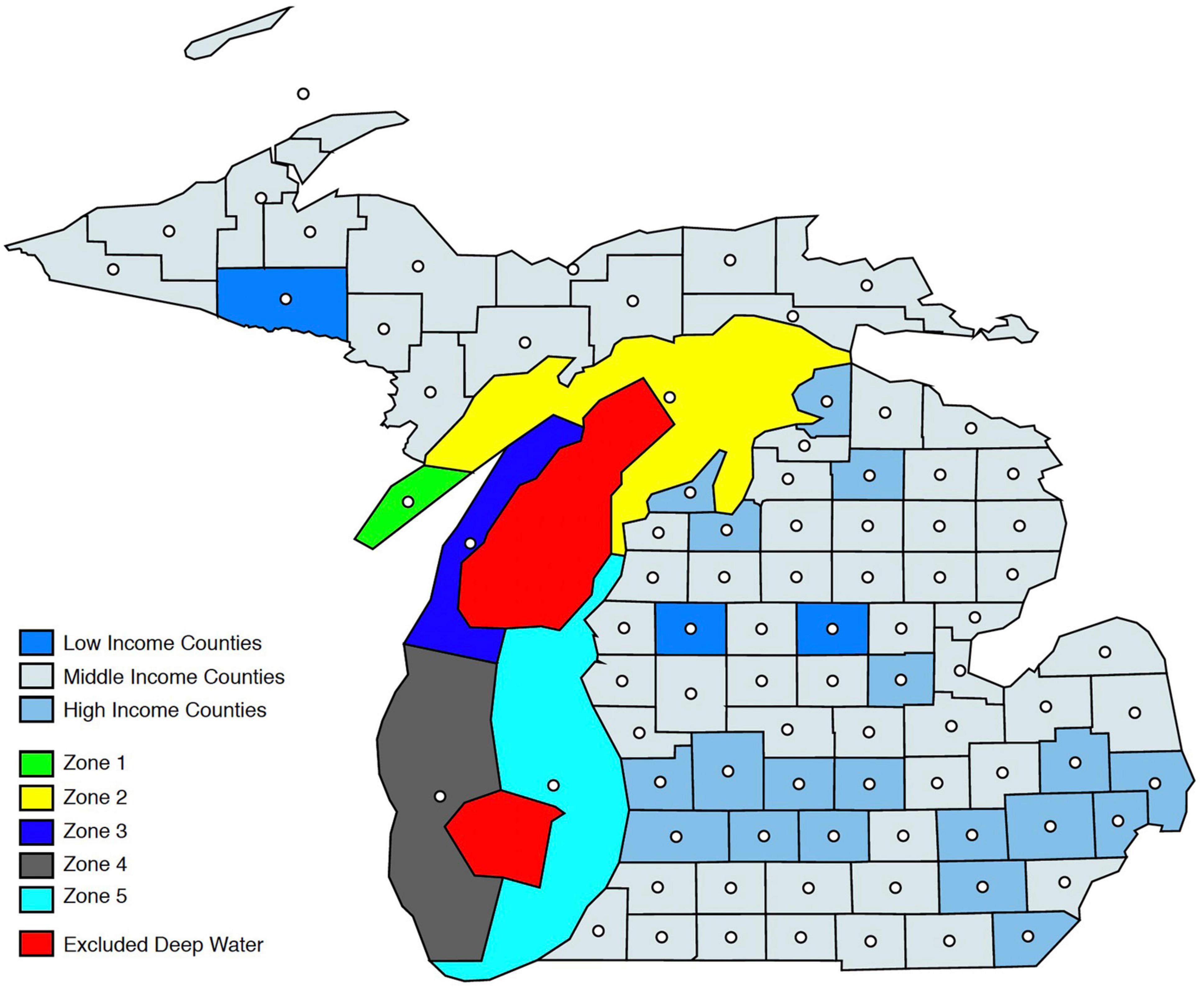
Figure 1. Geographic delineation of Lake Michigan ecological zones and counties by income level. White dots represent geographic centroids of counties and lake zones, used in distance calculations.

Altogether, the bioeconomic model is built by linking an economic decision model with an ecological model that generates species biomass data for both an invasion of bigheaded carp setting, and a non-invasion setting (Figure 2) for nine sportfishing species. Discussed in the remainder of this section are the theoretical economic and ecological models that when combined form the bioeconomic model, which is calibrated using ecological and economic data. The simulation process is defined following the description of the data and calibration.

FIGURE 2

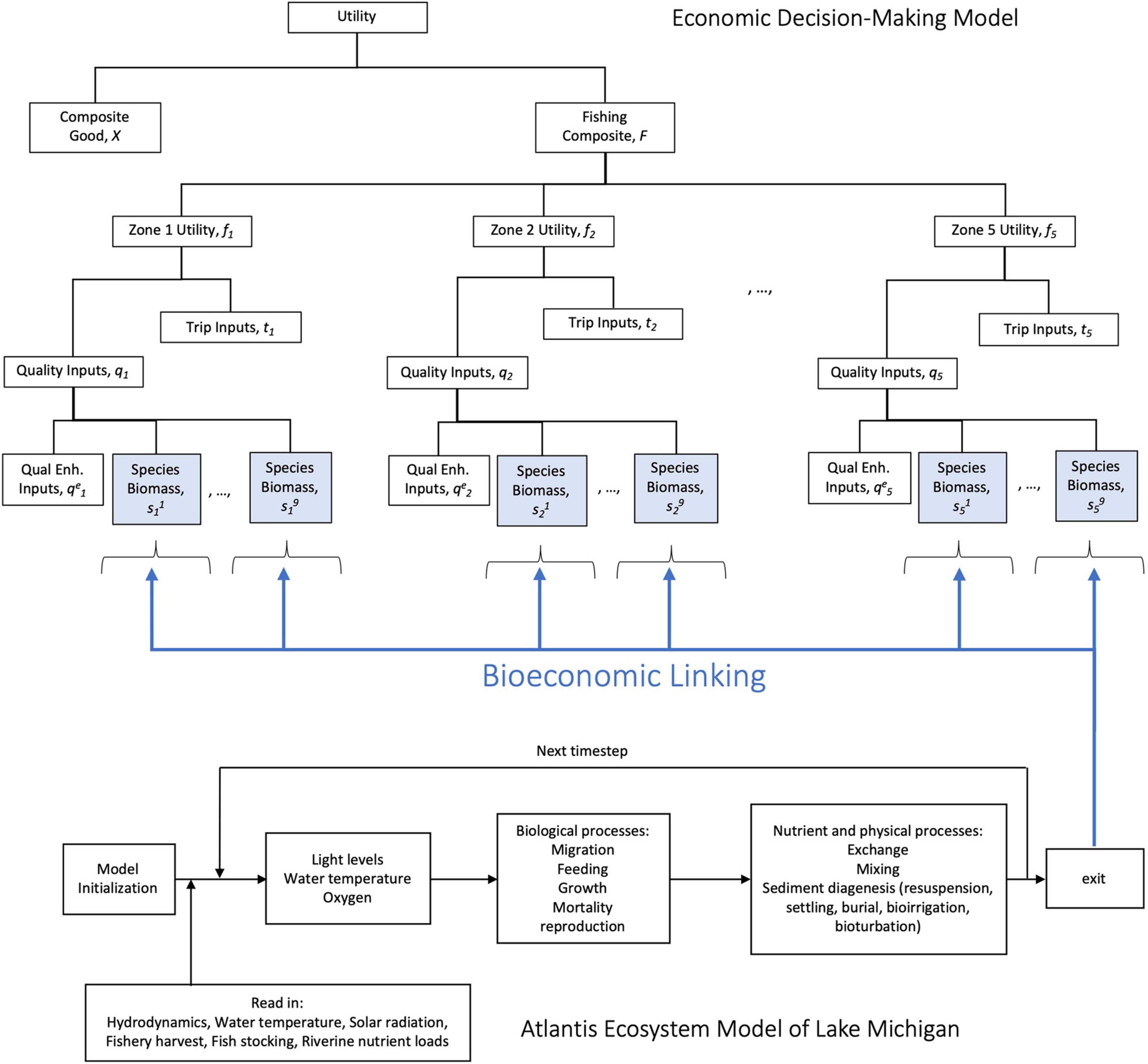
Figure 2. Schematic representation of the Bioeconomic Model. Economic utility or wellbeing is a nested function of space and species-specific decisions, which depend on the linked ecological models – the complex Atlantis model, or the simplified model.

Theoretical Economic Model

The bioeconomic model links the ecological and economic systems through the recreational fishing behavior of a representative consumer (henceforth, representative fisherman) from a representative household division. The fisherman derives utility – a metric representing satisfaction or wellbeing – from consumption of fishing and all other available societal goods. A nested utility framework (Ballard et al., 1985; Varian, 1992; Carbone and Smith, 2013) is used to incorporate the spatial representation of fishing behavior – that is, the desire to fish across different zones of Lake Michigan. The fisherman maximizes their utility (henceforth, wellbeing) by choosing where to fish, how much to invest in fishing related goods, and how much to consume of all other goods, subject to their overall budget².

Each representative fisherman’s wellbeing is comprised of four levels (Figure 2) of decision making. The decision made in the first level of the nest is their tradeoff between consumption of a composite good made up of all other societal goods (henceforth, the “composite good”) and composite recreational fishing consumption. Composite recreational fishing in level two is defined by how much the fisherman chooses to fish in each of zones. Fishing in any zone requires making the decision in level three of how many trips to take there and the fisherman’s perceived level of fishing quality there. In the fourth (or final) level, the fisherman produces their own perceived quality of the experience at each location, following Bockstael and McConnell (1981), by combining quality-enhancing inputs with zone-specific levels of species biomass. Quality-enhancing inputs are market purchases that improve the experience of fishing for specific species within that zone (e.g., bait, lures, or boat rentals). The link between the economic and ecological system is made in this fourth level. The ecological model forecasts the zone-specific levels of biomass for sportfishing species in Lake Michigan under invasion and non-invasion scenarios; it is this output that gets linked to the economic system to understand changes in fishing behavior in response to the invasion.

Identifying demand – or consumption decision rules – for each specific fishing variable follows from solving each nest-level optimization problem simultaneously. The optimization problem for each nest is discussed in turn, starting with level one. Here, the fisherman chooses total recreational fishing F and composite good consumption X, subject to their budget, such that the optimization problem is:

$$\underset{F,X}{\mathit{max}}U={\left(\mathrm{\theta }{F}^{\frac{({\mathrm{\sigma }}_u-1)}{{\mathrm{\sigma }}_u}}+\left(1-\mathrm{\theta }\right)X^{\frac{({\mathrm{\sigma }}_u-1)}{{\mathrm{\sigma }}_u}}\right)}^{\frac{{\mathrm{\sigma }}_u}{({\mathrm{\sigma }}_u-1)}}(1)$$

$$s.t.Y=p_{F}F+p_{X}X,(2)$$

In which Y is the fisherman’s income, p_F is the price of fishing, and p_X is the price of the composite good. Overall wellbeing is modeled using a constant elasticity of substitution functional form – a flexible form that embeds other standard utility functions used in economic modeling. When using this functional form, the multiplicative parameters for decision variables define the share that each represents in the output variable. Thus, the share of fishing consumption in overall wellbeing is θ and the share of the composite good is (1-θ). The ease at which the fisherman substitutes, or tradeoffs, between fishing and the composite good in response to price changes is defined by the elasticity of substitution parameter, σ_u. Elasticity of substitution in the broadest sense is the fisherman’s sensitivity and responsiveness to changes in prices.

The solution to (1) and (2) yields the consumption decisions for fishing and composite goods, which are derived from the first-order conditions:

$$F={\left(\frac{\mathrm{\theta }}{p_F}\right)}^{{\mathrm{\sigma }}_u}\frac{Y}{{\mathrm{\theta }}^{{\mathrm{\sigma }}_u}{p}_F^{\left(1-{\mathrm{\sigma }}_u\right)}+{\left(1-\mathrm{\theta }\right)}^{{\mathrm{\sigma }}_u}{p}_X^{\left(1-{\mathrm{\sigma }}_u\right)}},(3)$$

$$X={\left(\frac{1-\mathrm{\theta }}{p_X}\right)}^{{\mathrm{\sigma }}_u}\frac{Y}{{\mathrm{\theta }}^{{\mathrm{\sigma }}_u}{p}_F^{\left(1-{\mathrm{\sigma }}_u\right)}+{\left(1-\mathrm{\theta }\right)}^{{\mathrm{\sigma }}_u}{p}_X^{\left(1-{\mathrm{\sigma }}_u\right)}}.(4)$$

At the next level of the nest, the fisherman chooses fishing consumption in each zone, f_z, to maximize composite fishing consumption. The optimization problem is:

$$\underset{f_z}{\mathit{max}}F=\sum _z{\left({\mathrm{\beta }}_z{f}_z^{\frac{({\mathrm{\sigma }}_F-1)}{{\mathrm{\sigma }}_F}}\right)}^{\frac{{\mathrm{\sigma }}_F}{\left({\mathrm{\sigma }}_F-1\right)}}(5)$$

$$s.t.{\mathit{\text{Y}}-\mathit{\text{p}}}_{X}X=p_{F}F=\sum _z{p}_{fz}{f}_z.(6)$$

The share that each zone represents in overall fishing is β_z, and the elasticity of substitution between zones is σ_F. In (6) the price of fishing in each zone is p_fz and the budget available for spending on zone-level fishing is whatever the fisherman allocates to fishing overall (p_FF or equivalently Y−p_XX) as determined by the optimization at the previous level of the nest. The solution to (5) and (6) yields the following consumption decisions from the first-order conditions for zone-level fishing:

$$f_z={\left(\frac{{\mathrm{\beta }}_z}{p_{fz}}\right)}^{{\mathrm{\sigma }}_F}\frac{Y-p_{X}X}{{\sum }_z{\mathrm{\beta }}_z^{{\mathrm{\sigma }}_F}{p}_{fz}^{(1-{\mathrm{\sigma }}_F)}}\forall \text{z}.(7)$$

The optimization at the third level of the nest,

$$\underset{t_z,q_z}{\mathit{max}}{f}_z={\left({\mathrm{\alpha }}_z{\left(t_z\right)}^{\frac{({\mathrm{\sigma }}_z-1)}{{\mathrm{\sigma }}_z}}+\left(1-{\mathrm{\alpha }}_z\right){\left(q_z\right)}^{\frac{({\mathrm{\sigma }}_z-1)}{{\mathrm{\sigma }}_z}}\right)}^{\frac{{\mathrm{\sigma }}_z}{\left({\mathrm{\sigma }}_z-1\right)}}\forall \text{z},(8)$$

$$s.t.{\mathit{\text{Y}}-\mathit{\text{p}}}_{X}X-\sum _j{p}_{f_j}{f}_j=p_{f_z}{f}_z=p_{t_z}(d_z)t_z+p_{q_z}{q}_z,j\ne z,\forall \text{z},(9)$$

Defines the fisherman’s trip t_z and quality input q_z decisions, which are used to produce their zone-level fishing experience at each zone:

$$t_z={\left(\frac{{\mathrm{\alpha }}_z}{p_{t_z}(d_z)}\right)}^{{\mathrm{\sigma }}_z}\frac{Y-p_{X}X-{\sum }_j{p}_{f_j}{f}_j}{{\mathrm{\alpha }}_z^{{\mathrm{\sigma }}_z}{p}_{t_z}{(d_z)}^{\left(1-{\mathrm{\sigma }}_z\right)}+{\left(1-{\mathrm{\alpha }}_z\right)}^{{\mathrm{\sigma }}_z}{p}_{q_z}^{\left(1-{\mathrm{\sigma }}_z\right)}},$$

$$j=1,\mathrm{\hspace{0.33em}2},\mathrm{\dots }5,j\ne z,\forall z,(10)$$

$$q_z={\left(\frac{1-{\mathrm{\alpha }}_z}{p_{q_z}}\right)}^{{\mathrm{\sigma }}_z}\frac{Y-p_{X}X-{\sum }_j{p}_{f_j}{f}_j}{{\mathrm{\alpha }}_z^{{\mathrm{\sigma }}_z}{p}_{t_z}{(d_z)}^{\left(1-{\mathrm{\sigma }}_z\right)}+{\left(1-{\mathrm{\alpha }}_z\right)}^{{\mathrm{\sigma }}_z}{p}_{q_z}^{\left(1-{\mathrm{\sigma }}_z\right)}},$$

$$j=1,\mathrm{\hspace{0.33em}2},\mathrm{\dots }5,j\ne z,\forall z(11)$$

This modified household production function approach (Kolstad, 2011) is a way to introduce spatial decision making within a nested framework. Like the previous optimization steps, α_z is the share of trip inputs in production, (1−α_z) is the share of quality inputs, the elasticity of substitution between the two inputs is σ_z, the unit cost of a quality input is p_{q_z}, and the budget is the remainder from the previous optimization. The unit cost of a trip, p_tz(d_z), explicitly depends on the fisherman’s specific location in space, or the distance they must travel to the zone; the determination of this relationship is discussed in more detail in the following subsection.

The fourth and final nest is also an application of a household production function approach. Here, the fisherman combines quality-enhancing inputs $q_z^e$ with levels of species biomass $s_z^b$ to produce zone-level environmental quality, such that the optimization problem is:

$$\underset{q_z^e,s_z^b}{\mathit{max}}{q}_z={\left({\varphi }_{qe}{\left(q_z^e\right)}^{\frac{({\mathrm{\sigma }}_{qes}-1)}{{\mathrm{\sigma }}_{qes}}}+\sum _b{\varphi }_b{\left(s_z^b\right)}^{\frac{({\mathrm{\sigma }}_{qes}-1)}{{\mathrm{\sigma }}_{qes}}}\right)}^{\frac{{\mathrm{\sigma }}_{qes}}{({\mathrm{\sigma }}_{qes}-1)}}(12)$$

$$s.t.{\mathit{\text{Y}}-\mathit{\text{p}}}_{X}X-\sum _j{p}_{f_j}{f}_j-p_{t_z}(d_z)t_z+\sum _b{p}_{s_z^b}{s}_z^b=p_{q_z^e}{q}_z^e+$$

$$\sum _b{p}_{s_z^b}{s}_z^b,j\ne z,\forall \text{z}(13)$$

The share of quality-enhancing inputs in production is ϕ_qe and the share of each individual species in production is ϕ_b; it is a requirement of the functional form that all ϕ parameters sum to one. The elasticity parameters at this level are σ_qes. Residual budgeting follows the same convention as the previous nests and the price of quality-enhancing inputs is p_{q_z^e}.

This level of the nest is distinctly different because it includes a non-market input that links it to the ecological system: species biomass. Species biomass is a non-market good because it is not bought or sold in the traditional sense of an economic market; there is no market from which a price can be determined for species biomass and even if a supposed price could be assigned there is no market for exchange. Therefore, a “virtual” pricing framework as described in Carbone and Smith (2013) is used to develop a “virtual” market for species biomass. The framework endows the fisherman with “virtual” income to be spent only on species biomass and assigns “virtual” prices to species based on willingness to pay estimates from empirical analysis. With this approach the representative fisherman responds to changes in species biomass the same way they would in a traditional market. For example, if a species becomes more scarce the “virtual” price for that species increases and vice versa. Thus, any shift in demand for a particular species will cause a shift in demand for quality-enhancing inputs in the fourth level of the nest, linking the non-market behavior to other economically driven behaviors.

The virtual prices, p_{s_z^b}, used here are willingness to pay estimates and the fisherman’s endowment of virtual income, to be spent on species biomass only, is ${\sum }_b{p}_{s_z^b}{s}_z^b$ Under these assumptions, the solution to (12) and (13) generates the demand for quality-enhancing inputs,

$$q_z^e={\left(\frac{{\mathrm{\varphi }}_{qe}}{p_{q_z^e}}\right)}^{{\mathrm{\sigma }}_{qes}}\frac{Y-p_{X}X-{\sum }_j{p}_{f_j}{f}_j-p_{tz}{t}_z+{\sum }_b{p}_{s_z^b}{s}_z^b}{{\mathrm{\varphi }}_{qe}^{{\mathrm{\sigma }}_{qes}}{p}_{q_z^e}^{(1-{\mathrm{\sigma }}_{qes})}+{\sum }_b{\mathrm{\varphi }}_b^{{\mathrm{\sigma }}_{qes}}{p}_{s_z^b}^{(1-{\mathrm{\sigma }}_{qes})}},j\ne z,\forall z(14)$$

And the demand for species biomass,

$$s_z^b={\left(\frac{{\mathrm{\varphi }}_b}{p_{s_z^b}}\right)}^{{\mathrm{\sigma }}_{qes}}\frac{Y-p_{X}X-{\sum }_j{p}_{f_j}{f}_j-p_{tz}{t}_z+{\sum }_b{p}_{s_z^b}{s}_z^b}{{\mathrm{\varphi }}_{qe}^{{\mathrm{\sigma }}_{qes}}{p}_{q_z^e}^{(1-{\mathrm{\sigma }}_{qes})}+{\sum }_b{\mathrm{\varphi }}_b^{{\mathrm{\sigma }}_{qes}}{p}_{s_z^b}^{(1-{\mathrm{\sigma }}_{qes})}},j\ne z,\forall z\forall b(15)$$

An implication of the non-market components of the model is that prices from nest to nest must be endogenously determined to maintain consistency. The only prices determined in markets are those for trip-related expenditures (e.g., gas, lodging, and time) and quality-enhancing purchases (e.g., bait, lures, and rentals)³. All other prices are found using unit expenditure functions from the optimization problem. For example, the price of composite fishing p_F is given by the unit expenditure on fishing ex_F found from (5) and (6) as:

$$e{x}_F=p_F={\left(\sum _z{\mathrm{\beta }}_z{p}_{fz}^{(1-{\mathrm{\sigma }}_F)}\right)}^{\frac{1}{(1-{\mathrm{\sigma }}_F)}}(16)$$

The same applies for the price of fishing in each zone, p_{f_z}, and the price of quality inputs, p_{q_z}.

Theoretical Ecological Models

Discussion now turns to the development of the ecological models that link to the economic decision model and complete the full bioeconomic model. There are two types of ecological models used in this analysis – a complex ecological model that considers many layers of the ecological system, the Atlantis Ecosystem Model, and a simplified model (henceforth, non-Atlantis) that lacks certain details of the ecological system, mimicking models used in economic analyses. Both models include spatially explicit zone characteristics, but of varying degree. Only the Atlantis model accounts for interactions between species at different levels of the food web.

Atlantis Ecosystem Model

The Atlantis ecosystem model is a three-dimensional, spatially explicit, end-to-end ecosystem model, that includes hydrodynamics, nutrient cycling, trophic dynamics all the way from primary producers to apex predators and to fisheries with various levels of complexity (Fulton et al., 2004; Olsen et al., 2018) to quantitatively evaluate ecosystem responses to natural or anthropogenic stressors or management scenarios to support resource management decision-making (Fulton et al., 2011). The Atlantis ecosystem model provides predictions of indirect trophic effects on species under ecosystem perturbations.

Our Atlantis ecosystem model focuses on the trophic dynamics submodule to address Lake Michigan food web responses to the bigheaded carp invasion and takes daily input of water exchange, water temperature, surface light conditions, nutrient loading, fishery harvest, and fish stocking, and runs the food web on a 3-dimensional structure of 35 horizontal polygons and up to six vertical layers with a timestep of 6 h. The model’s spatial resolution is mainly based on the bathymetry (30 and 110 m isoclines) and fishery management boundaries. The food web includes 38 model groups, including fish, zooplankton, benthic invertebrate, primary producers, and bacteria.

The ecological processes are briefly described below – for detail see the model user guide (Audzijonyte et al., 2017). Bacteria include pelagic bacteria and benthic bacteria, and bacteria biomass is dynamically simulated as a function of detritus biomass. Mortality of bacteria is caused by predation or grazing by different consumers, and other optional conditions such as, oxygen limitation, acidification. The wastes from bacteria are refractory detritus, DON and NH3, which are part of the nitrification-denitrification and remineralization processes. Nutrients of nitrogen, silicon, and phosphorus are tracked in the Atlantis, but nitrogen is the common currency.

Primary producers include phytoplankton and benthic algae. Their growth (G_PP) is simulated as a function of maximum growth rate (μ_PP), water temperature scalar (T_scalar), light limitation (δ_irr), nutrient limitation (δ_N), and space limitation (δ_space) and population biomass (17). The changes in population biomass of primary producer (d(PP)/dt) are a function of growth (G_PP), predation mortality (M_i,PP), lysis mortality (M_lysis), linear mortality (M_l), quadratic mortality (M_q), and transport out (E_out) or back in (E_in) the biomass pool:

$$G_{PP}={\mathrm{\mu }}_{PP}\cdot T_{scalar}\cdot {\mathrm{\delta }}_{irr}\cdot {\mathrm{\delta }}_N\cdot {\mathrm{\delta }}_{space}\cdot PP(17)$$

$$\frac{d\left(PP\right)}{dt}=G_{PP}-\sum _{i=predators}{M}_{i,pp}-M_{lysis}-M_l-M_q-E_{out}+E_{in}(18)$$

Invertebrate consumers – zooplankton and benthos – are simulated as aggregated biomass pools in each model cell with biological processes of growth, predation, and linear and quadratic mortality. Fish species are modeled with multiple age classes. The number of fish individuals and their average weight are tracked for each age class and each spatial model cell through time. Biological and ecological processes that are simulated for fish include growth, consumption, predation, reproduction, movement, migration, and linear and quadratic mortality. The quadratic mortality represents density dependent mortality (e.g., disease) that are not explicitly modeled, which may impose a reasonable carrying capacity. Fish recruitments either followed the Beverton–Holt model or the Ricker model (Brown et al., 1993; Brenden and Bence, 2009).

The changes in population biomass of consumers (d(CP)/dt) are a function of growth (G_CP), predation mortality (M_i,CP), linear mortality (M_l), quadratic mortality (M_q), and transport/migration out (E_out) or back in (E_in) the biomass pool, and fishing mortality (F_CP) for fishery species:

$$\frac{d(CP)}{dt}=G_{CP}-{\sum }_{i=predators}{M}_{i,CP}-M_l\cdot T_{scalar}-M_q\cdot$$

$$T_{scalar}-E_{out}+E_{in}-F_{CP}(19)$$

Growth is a function of consumption (C), water temperature, and prey-type specific assimilation rates. The consumption is a Holling type II function (Miller et al., 1992; Ray and Corkum, 1997).

$$C_{ij}=\frac{C{P}_i\cdot {\mathrm{\alpha }}_{ij}\cdot C{P}_j\cdot C_{max}}{1+\frac{C_{max}}{g}{\sum }_j(E_{ij}\cdot T_{scalar}\cdot C{P}_j\cdot {\mathrm{\alpha }}_{ij})},(20)$$

In which C_ij is consumption of i on prey j, α_ij is the availability of prey j to predator i, C_max is the maximum ingestion rate of predator i, g is the maximum growth rate of predator i, E_ij is efficiency of predator i on prey j and is temperature dependent. The spatial biomass distribution of species is dependent on productivities, food webs, and predefined seasonal distributions of fish species across zones that is always proportional to the total fish population⁴. Output of the model is zone-specific biomass data (g/m²) for each sportfishing species included in the model for a 25-year period, 2015–2040.

Simplified Ecological Model (Non-Atlantis)

The simplified, non-Atlantis ecological model is developed to mimic the type of model sometimes used in economics that make simplifying assumptions about space or species interactions. A model is constructed where each species exhibits logistic growth in the non-invasion state following in which s^b is species-specific biomass, r^b is species-specific intrinsic growth, and ^Kb the species-specific carrying capacity.

$$\frac{d{s}^b}{dt}=r^b*s^b\left(1-\frac{s^b}{K^b}\right),(21)$$

To generate species biomass in the invasion state, only a single interaction between the species and bigheaded carp, c, is included. The growth function in the invasion state, following the Lotka-Volterra form (Hastings, 2013), is:

$$\frac{d{s}^b}{dt}=r^b*s^b\left(1-\frac{s^b}{K^b}\right)+{\mathrm{\alpha }}^b{s}^{b}c.(22)$$

The invader benefits some species and harms others, and thus the interaction parameter, α^b, can either be positive or negative. Each species’ growth function and carrying capacity differ based on the specific zone (i.e., spatially explicit zone characteristics), while the intrinsic growth rates and bigheaded carp effects are not assumed to be zone dependent. In comparison to the Atlantis model, the non-Atlantis model lacks the multiple levels of detail related to spatially explicit ecological characteristics and all species-specific interactions within the food web.

Data and Calibration

Economic and Geographic Data

The data available for this analysis does not allow for empirical identification. It does, however, provide enough information to calibrate and parameterize the model described in the previous section to a set of representative consumers (i.e., fishermen) within the regional economy of Lake Michigan. The calibrated model is used to assess realistic responses to changes in ecosystem characteristics and metapopulations. The main source of economic data is annual data for the state of Michigan from IMPLAN (2014)⁵. IMPLAN tracks economic exchanges between household income divisions, industries, and governmental agencies. This economic data is used to identify income after taxes and savings and expenditures on goods and services. Though quite comprehensive, IMPLAN does not collect information specific to recreational fishing. The “National Survey of Fishing, Hunting, and Wildlife – Associated Recreation (NSFHWA)” (U.S. Department of the Interior, Fish and Wildlife Service, and U.S. Department of Commerce, 2011) is used to identify expenditures on trip and quality related fishing expenses. The final source for economic data is Melstrom and Lupi (2013), which provides the willingness to pay estimates used as the virtual prices for the sportfishing species considered in this analysis: – burbot (Lota lota), Chinook salmon (O. tshawytscha), Coho salmon (O. kisutch), lake trout (S. namaycush), lake whitefish (Coregonus clupeaformis), rainbow smelt (O. mordax), steelhead (rainbow trout, O. mykiss), walleye (Sander vitreus), and yellow perch (Perca flavescens) (Table 1). There were three species not estimated in Melstrom and Lupi (2013); these species were assigned the lowest estimated willingness to pay in the benchmark to avoid overstatement of results though an additional analysis is performed to understand how sensitive the model is to this assumption. Because the willingness to pay is equivalent to the virtual price, the remainder of the analysis uses the willingness to pay designation.

TABLE 1

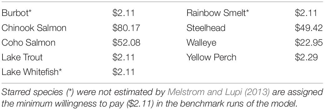
Table 1. Willingness to pay estimates.

Additional data sources were needed to compile the geographic information for representative fishermen’s location in space. Since IMPLAN delineates household divisions by income, some measure of income based in space is needed to match a household division to a location. This information is collected from the 2016 American Community Survey (U.S. Census Bureau, 2018), which lists average income for each state, by county. Average county income is then matched to a respective household income division from the IMPLAN data. Using geographic information systems and Census Bureau shapefiles, the geographic centroid of each county – now household division-specific – and each lake zone is identified (Figure 1). The distance (in miles) between the county and lake centroids is calculated and converted into a unit cost of travel to that zone for each household division (Supplementary Table 1). The unit costs are found by taking the total expenditures on travel (e.g., gas and lodging), by household division, as reported in the NSFHWA survey, and dividing by total miles traveled. It is important to note that range of average incomes across counties in Michigan is rather small – the range is $31,000–$77,000. This constrains the analysis to consideration of just three income divisions and, thereby, a representative fisherman for each household income division: Low-Income (≤$35,000), Middle-Income ($35,000–$50,000), and High-Income (≥$50,000).

The final data used in the economic model is output from the two types of ecosystem models – the non-Atlantis model which excludes species interactions, and the complex, Atlantis model with full interactions and spatial characteristics.

Ecological Data

The data for the Atlantis ecosystem model of Lake Michigan, come from a variety of sources (see Supplementary Tables 2–4). Times series biomass data including zooplankton groups are from the Great Lake National Program Office monitoring program; dreissenid mussel data is from NOAA Great Lakes Environmental Research Lab; fish biomass data is from the USGS Great Lakes Science Center; and salmonines from Rogers et al. (2014). The flux of water and heat across each model box and depth layer is governed by a 3-dimensional circulation model of Lake Michigan (Beletsky and Schwab, 2008). Fishery harvest and fish stocking are from the Great Lakes databases at the Great Lakes Fishery Commission. Finally, the tributary nutrient loads are from the University of Wisconsin (M. Rowe at NOAA Great Lakes Environmental Research Laboratory, personal communication).

Calibration

The ecosystem models and the full bioeconomic model are calibrated to represent the observed ecological and economic conditions in Lake Michigan and its regional economy. To calibrate Atlantis, the following steps were completed as suggested by the model developers: (1) No species go extinct, except extinction observed in the field during the simulation periods. (2) Simulated vertebrates have a reasonable size-at-age. (3) Model simulations are compared with historical observations if available. (4) For species with no historical observations, ensure the simulated population dynamics are reasonable. (5) If spatial distributions are available, compare modeled spatial distributions with the observations. Model simulated biomass for 19 model groups are compared to field estimates of lake-wide biomass. Finally, the spatial distribution across different depths were calibrated for dreissenid mussel biomass using observations from Ashley Elgin at NOAA Great Lakes Environmental Research Lab. Given the complexity of the ecosystem and short period of observation, available observation data are used to iteratively calibrate the model acting as the closest means of a verification process as possible, which are often missing for such models (Fulton et al., 2004; Kaplan et al., 2010; Kao et al., 2018). The Atlantis model was initiated in 1994 and calibrated from 1994 to 2015. The model continued to run for a total of 25 years under the same forcing levels of the last available year. Bigheaded carp were added into the Atlantis model, and parameter values were based on Zhang et al. (2016). To understand the implications of the bigheaded carp invasion, the Atlantis model is run with the bigheaded carp simulated ecosystem changes and then without the bigheaded carp effects which generates non-invasion and invasion biomass data.

For the non-Atlantis ecological model, which is used to depict models applied in economic literature, all species-specific parameters for intrinsic growth and zone-specific initial biomass are drawn from Zhang et al. (2016) and Finnoff et al. (2019). Data was not readily available for the zone-specific carrying capacities; therefore, the maximum values of biomass recorded in the output from the Atlantis are used as a proxy. Lastly, the interaction parameters are calibrated using the mean changes in biomass from Zhang et al. (2016).

The full bioeconomic model is calibrated for three representative fisherman that are differentiated by income level and fishing behavior. There is a low-income household division, a middle-income household division, and a high-income household division. The calibration technique used in this analysis employs the calibrated share form from Rutherford (2002). Using benchmark values for all demands, prices, costs of production, and output, the only assumed parameters are the elasticities of substitution. All other parameters can be solved for – or calibrated – at the benchmark (i.e., θ, β, α, ϕ)⁶.

Simulation Analysis Framework

The ecological models are used to consider the four different specifications of the full bioeconomic model that are assessed in the comparative analysis: (1) Atlantis with spatially heterogenous zones; (2) non-Atlantis with spatially heterogenous zones; (3) Atlantis with spatially homogenous zones; (4) non-Atlantis with spatially homogenous zones. Because both the Atlantis and non-Atlantis models include explicitly spatial ecological characteristics in their parameterization, the biomass output from these models directly define the spatially heterogenous zone data used in specifications (1) and (2). To derive the spatially homogenous zone data for specifications (3) and (4), the spatial characteristics are aggregated and averaged and then each zone is treated as ecologically identical. Specifically, the average population biomass for each species across the fives zones for each year for each ecological model is calculated and then assigned to all five zones making them spatially homogenous. The four different model specifications are run forward for 25 years from 2015 and for a non-invasion scenario in which bigheaded carp do not invade Lake Michigan and an invasion scenario in which they do.

To assess the implications of the bigheaded carp invasion, estimates of changes in the fisherman’s wellbeing (or social welfare) are calculated for each year in the analysis – by comparing overall social wellbeing in the non-invasion and invasion states. The social welfare metric is compensating variation, which defines how much compensation ($ year^–1) the representative fisherman from each household division would need to be given to make up for lost wellbeing from the ecological consequences of the invasion. Higher dollar estimates correspond to greater compensation needed for losses in wellbeing. The comprehensive metric used in this analysis is the aggregate compensation – the sum over all household divisions and years – discounted at 5%⁷, also referred to as the net present value of the welfare losses. The net present value of welfare loss is the sum of today’s losses and all discounted losses into the future. This metric is calculated and compared across the different ecological specifications (i.e., spatial heterogeneity or homogeneity, and Atlantis or non-Atlantis) to demonstrate the implications of including species interactions and spatially heterogenous ecological characteristics.

An additional comparative analysis is performed to understand how the consequences from oversimplified assumptions are exacerbated or attenuated by changes in the fishermen’s (1) responsiveness to prices and willingness to substitute between species (i.e., the elasticity of species and quality substitution) at the lowest level of the utility nest and (2) willingness to pay values for species biomass. The benchmark value of the elasticity of substitution between species and quality-enhancing inputs is 0.9. The four alternatives considered are increases and decreases of 25%, a decrease of 50%, and an increase of 100% (i.e., 0.45, 0.675, 1.125, and 1.8). The three additional willingness to pay (WTP) considerations assign the average WTP ($23.93) to all species; assign the average WTP to just the three species not estimated in the Melstrom and Lupi (2013) analysis; assign the highest WTP to the three species not estimated ($80.17).

The final analysis considers hypothetical implementation of a protected area policy, in which one lake zone is established as a protected area that is spared from the ecological consequences of the invasion. It is acknowledged that this policy may not be the most effective, nor the easiest to implement in the bigheaded carp setting, yet it is a feasible policy to consider in the scope of this analysis and is sufficient to generalize biases in policymaking from simplified assumptions. Each individual zone, under each ecological specification is evaluated as a protected area. In this demonstrative analysis the zone that generates the greatest benefit (in terms of improved wellbeing) is assigned the protected area designation⁸.

Results

This section presents the results of the comparative analyses with respect to species interactions, spatial characteristics, fisherman responsiveness and preferences, and policy assessments. Given the large volume of information across many different dimensions, a set of select species, zones, and economic outcomes are displayed in tables and figures in the main body to support the underlying result, all other figures or relevance are included in the Supplementary Material.

Atlantis (Species Interactions) vs. Non-Atlantis (No Species Interactions)

The results of the first comparative case – Atlantis (species interactions) and non-Atlantis (no species interactions) – illustrate the significant differences that can arise in estimates of social welfare loss if interactions between different layers of the ecosystem and food web are excluded from the analysis. For example, biomass predictions for Coho salmon and rainbow smelt are starkly different across all zones regardless of how the spatial characteristics are treated (i.e., spatially homogenous zones or spatially heterogenous zones) (Figure 3).

FIGURE 3

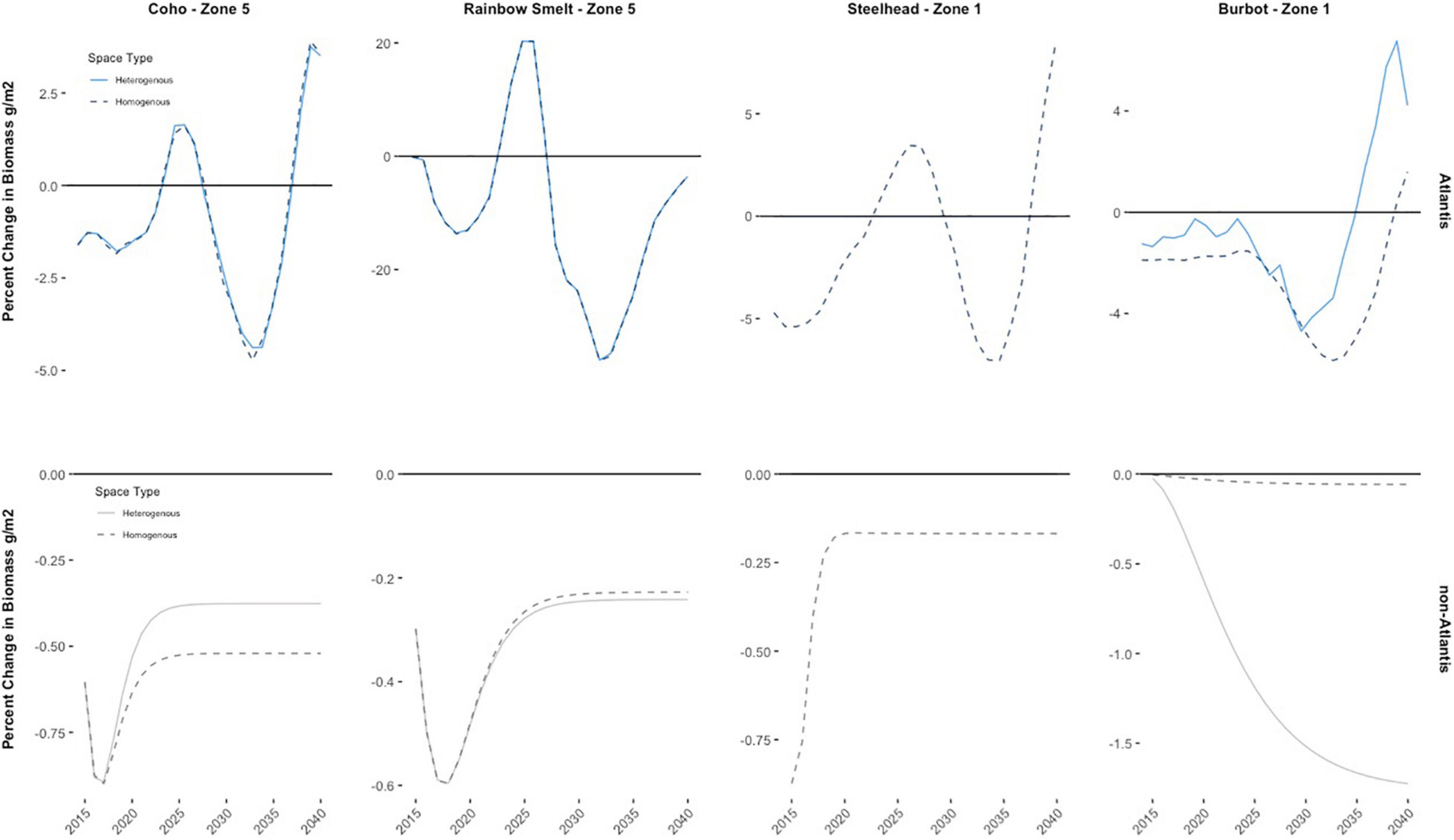
Figure 3. Yearly percent change in Coho salmon and rainbow smelt biomass in zone 5 and yearly percent changes in steelhead and burbot biomass in zone 1 due to the bigheaded carp invasion for all ecological specifications of the model – interactions (Atlantis ecosystem model), no interactions (the simplified ecological model), heterogenous zones, and homogenous zones. The homogenous specifications assume all zones are ecologically the same and, thereby, biomass values for all species are assigned the lake average biomass. Conversely, the heterogenous specification accounts for spatially explicit ecological characteristics; for example, here the specific characteristic is that steelhead biomass is not well-established in zone 1.

The results of the Atlantis model predict that most fish species at the beginning of the invasion are negatively impacted, yet as the invasion progresses the fish population biomass oscillates around zero indicating that the food web interactions can at times buffer or exacerbate changes in biomass from the invasion. For piscivorous fish species – such as Coho salmon, burbot, and steelhead – the invasion in later periods tends to have positive biomass effects due to increased predation on the bigheaded carp. Other species (i.e., rainbow smelt) experience more drastic and overall negative implications from direct food competition with bigheaded carp (Figure 3). These oscillations do not exist when using the non-Atlantis model which excludes species interactions. Results of the non-Atlantis model predict consistent – one-directional – biomass implications, which depend only on the species’ bigheaded carp interaction parameter which is negative for all species except lake whitefish and yellow perch⁹. Coho salmon, for example, do experience greater biomass loss in the early stages of the invasion but then reach a steady state of consistent year over year declines in biomass ranging from 0.4% (spatially heterogeneous zones) to 0.6% (spatial homogenous zones). Similar results hold for all other species when using the non-Atlantis specification (Figure 3).

The potential differences in magnitude and the direction of the impacts when comparing the non-Atlantis and Atlantis model results can be clearly demonstrated by the results for rainbow smelt. Rainbow smelt biomass varies by more than 20% (+/−) at times with the Atlantis model yet decreases by no more than 0.6% using the non-Atlantis model. Similarly, Steelhead vary more than 5% (+/−) when using Atlantis: almost five times the size of the largest yearly impact on Steelhead using the non-Atlantis model.

The lack of species interactions in non-Atlantis model leads to attenuated biomass effects of the bigheaded carp invasion and, thereby, attenuated impacts in terms of social welfare implications. The non-Atlantis model generates social welfare losses that are almost an order of magnitude smaller than the Atlantis model (Table 2). If using the non-Atlantis model, the discounted social welfare costs in terms of reduced fishermen wellbeing from the invasion range from $480,000 (spatially homogenous zones) to $510,000 (spatially heterogenous zones). If using the Atlantis model, the social welfare costs range from $9.31 million (spatially heterogenous zones) to $9.35 million (spatially homogenous zones). Though these estimates of social welfare are significantly different, one consistent result is that all ecological specifications do predict overall losses to fishermen wellbeing from the bigheaded carp invasion, which can be explained by the results of the different nests of the bioeconomic model (Figure 2). The responses of the representative fishermen across the model specifications are analogous and vary only in magnitude and in substitutions at the lowest level of the nest.

TABLE 2

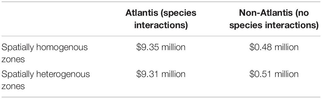
Table 2. Estimates of social welfare loss in millions of dollars – calculated as the net present value of the compensating variation metric.

Under the Atlantis specification, almost all species across all zones experience declines in population biomass on net over the time frame (see Supplementary Figures 7 and 9 for complete biomass tables), leading to similar implications for social welfare across households and zones. The representative fishermen respond to the increased scarcity of the sportfishing species by increasing their purchases of quality enhancing inputs needed to improve quality of fishing by zone and by increasing their willingness to pay for the species most negatively impacted by the invasion (e.g., rainbow smelt and lake whitefish) – rather than by increasing the species with the highest value (e.g., Coho or Chinook salmon) because it is too costly (Figure 4, left and middle column). Fishing quality becomes more expensive to achieve (Figure 4, middle column) for each zone and thus the representative fishermen are forced to reduce trips and quality demands due to their limited budget. Altogether, the fishing price for each zone increases (Figure 4, right column) causing the fishermen to fish less across all zones. Though, the reductions in fishing across zones does vary across spatial settings. When the zones are spatially heterogenous the fishermen’s costs increase most on average for zones 4 and 5 – about 0.28% for the low-income division, 0.55% for the middle-income division, and 0.07% for the high-income division. Costs increase most in zones 1 and 2 when using the spatially homogenous zones specification – about 0.3% for the low-income division, 0.63% for the middle-income division, and 0.08% for the high-income division. The overall reduction in fishing across zones in either specification results in the social welfare losses.

FIGURE 4

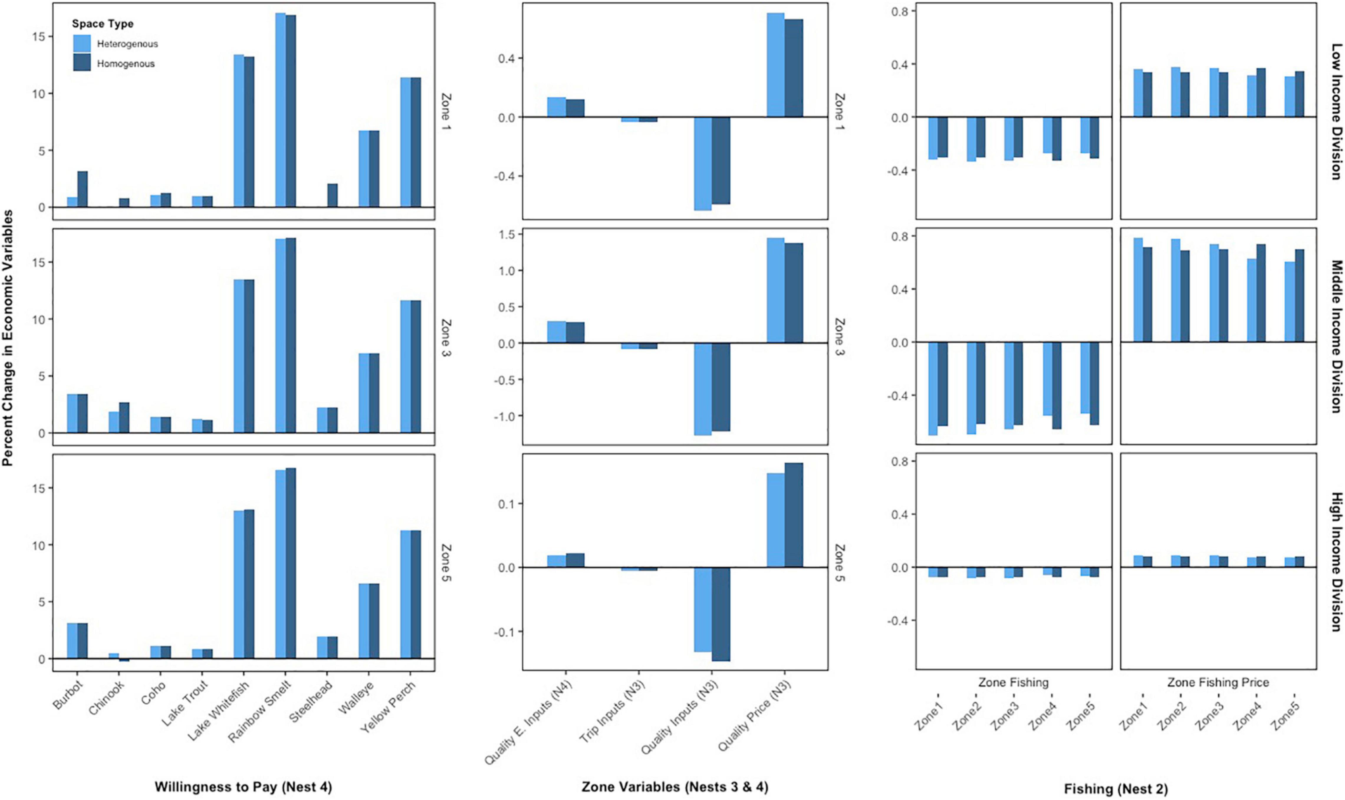
Figure 4. Percent changes in select recreational fishing responses for the Atlantis specifications. The left column displays willingness to pays for a specific zone for each household division and the middle column displays the quality and trip related responses for the same zone for each household. The right column displays overall zone-fishing response for all five zones. The nest labels correspond to the nested bioeconomic model in Figure 2. Additionally, two results were increased to be visible on the figure: trip inputs by a factor of 1000 and Chinook salmon by a factor of 10.

Generally, the results of the fishermen responses for the non-Atlantis model are the same: the fishing costs for each zone increase, leading to reduced fishing overall and losses in social wellbeing (Figure 5, right column). The key difference between the specifications is that more substitutions occur at the lowest level of the bioeconomic model (Figure 2). The representative fishermen decrease their willingness to pay for species that become more abundant in population biomass from invasion (e.g., lake whitefish and yellow perch), which gives the fishermen the ability to make more substitutions in terms of willingness to pay for the other sportfishing species (Figure 5, left column) and reduces the overall social welfare implications of the models.

FIGURE 5

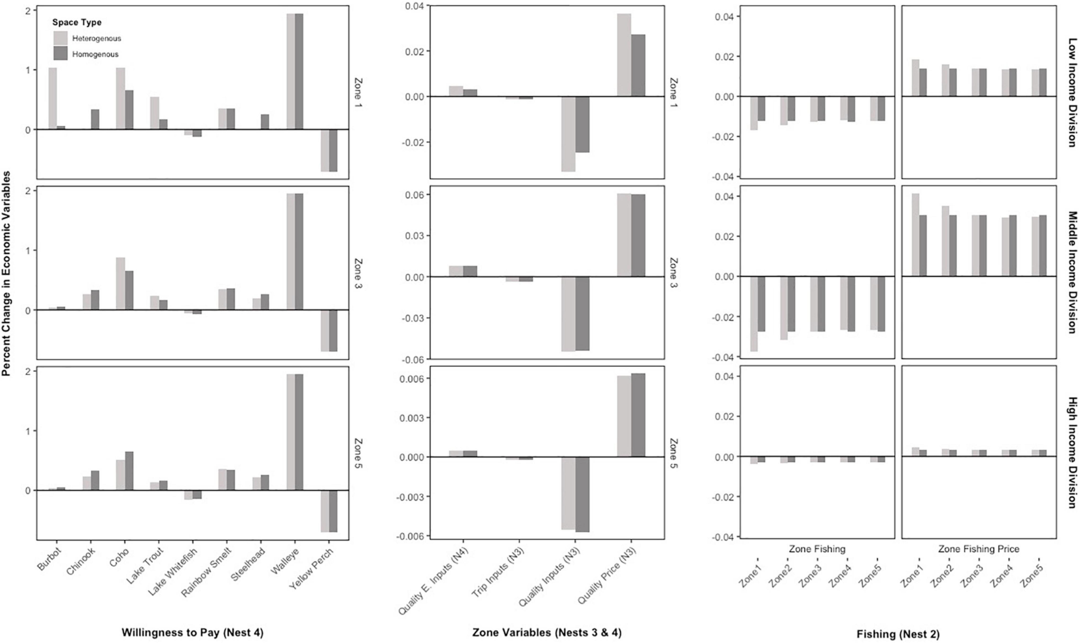
Figure 5. Percent changes in select recreational fishing responses for the non-Atlantis specifications. The left column displays willingness to pays for a specific zone for each household division and the middle column displays the quality and trip related responses for the same zone for each household. The right column displays overall zone-fishing response for all five zones. The nest labels correspond to the nested bioeconomic model in Figure 2. Additionally, three results were edited to be visible on the figure: trip inputs were increased by a factor of 1000, lake whitefish increased by a factor of 10, and walleye reduced by a factor of 10.

Spatially Homogenous Zones vs. Spatially Heterogenous Zones

There is no clear trend in the social welfare implications of the invasion when comparing spatially homogenous and spatially heterogenous zones. Here, the same ecological relationships and results hold for the output of the Atlantis and non-Atlantis models: piscivores are negatively impacted less, while all other species are negatively impacted more using Atlantis, and for non-Atlantis all species, aside from lake whitefish and yellow perch, are negatively impacted. However, aggregating the output of the two models and then assuming that all zones are spatially homogenous (i.e., ecologically identical) – as researchers tend to do if data is limited – has two major effects on the biomass results when comparing the Atlantis model and the non-Atlantis model. The first is that some species have biomass populations in zones where they are not well-established ecologically when treating space homogenously. For example, steelhead are not well-established in zone 1 because the habitat is warm, turbid water that is not well-suited for them; this spatial characteristic is observed in the spatially heterogenous specifications for both the Atlantis and non-Atlantis models. Yet, when spatially aggregating to treat all zones homogenously steelhead biomass populations artificially exist because all zones are assumed identical (Figure 3).

Second, the resultant aggregated biomass values in the spatially homogenous specifications for Atlantis and non-Atlantis output are influenced by outliers and by the variance in biomass predictions across zones, causing the aggregated biomass values to deviate from a representative mean. For example, burbot in zone 1 is more negatively skewed when treating all spaces homogenously using the Atlantis model, whereas burbot in zone 1 is skewed in a positive direction when treating spaces homogenously using the non-Atlantis model (Figure 3).

These two types of biomass results inform the divergence in social welfare computations for the comparison across spatially homogenous or heterogenous zones. Losses in social welfare are slightly lower if zones are treated as spatially homogenous instead of spatially heterogenous when using the non-Atlantis model; the aggregation underestimates the losses in welfare by approximately $30,000 (Table 2). Conversely, the aggregation overestimates losses by approximately $40,000 when treating the zones as spatially homogenous as compared to spatially heterogenous using Atlantis. Although the differences in the social welfare estimates are small for this specific analysis, they are the direct result of biases from aggregation, implying that spatial characteristics do matter, which is discussed in more detail in the “Discussion” section.

The social welfare losses again stem from the responses of the recreational fishermen at different levels of the bioeconomic model (Figure 2) which are analogous to the previous results: fishing for all species with Atlantis (or most species with non-Atlantis) becomes more expensive in all zones because population biomass levels fall from the invasion, leading to fewer trips, quality purchases, and fishing overall. Thus, the difference in social welfare estimates is dependent on how far the fishermen’s zone-level fishing responses deviate from the spatially heterogenous specification to the spatially homogenous specification. For example, when using the Atlantis model and treating zones as spatially homogenous, the costs of fishing increase in zones 4 and 5 and fall in zones 1, 2, and 3 for each household division, as compared to the spatially heterogenous zone specification (Figure 4, right column). The rise in costs in zones 4 and 5 are more significant, than the fall in costs for the other zones leading to the slightly higher social welfare losses when using homogenous zones and the Atlantis model. For the non-Atlantis specifications, the outcomes are just reversed. Costs are significantly reduced in zones 1 and 2, are marginally reduced in zone 3, and rise slightly in zones 4 and 5 (Figure 5, right column); the savings are greater than the added costs, and therefore the social welfare implications are better.

Fisherman Responsiveness and Preferences

The results have demonstrated that accounting for layers of interactions between species is important and that including the spatial ecological characteristics of the zone can matter for economic outcomes. However, the social welfare implications are also dependent on the value that the representative fishermen put on each species and the ease at which they are willing to make substitutions between species and quality-enhancing goods. Additional analysis is completed to understand how dependent the outcomes are on these additional parameters, and the results are presented in turn.

First considered is the representative fishermen’s ease at which they are willing and able to substitute between fish species and quality-enhancing goods in response to price changes from the invasion. Across the specifications that use the Atlantis model (e.g., Figure 6, left panel), the results are as expected. When it is more difficult for the fishermen to make substitutions (i.e., the parameter is lower than in the benchmark) the fishermen are worse off, and their social welfare losses from the invasion are greater than those in the benchmark. The opposite holds when the fishermen have more flexibility to make substitutions (i.e., a higher parameter value than the benchmark); fishermen are better off and the social welfare losses are lower. These results are also consistent for the specification that uses the non-Atlantis model and spatially heterogenous zones. The results from the spatially homogenous, non-Atlantis model specification, however, diverge from the others; it shows that making it more difficult to substitute generates better economic outcomes (or less social welfare loss), whereas making it easier to substitute generates slightly higher social welfare loss as compared to the benchmark (Figure 6, right panel). This result is discussed in more detail in the “Discussion” section.

FIGURE 6

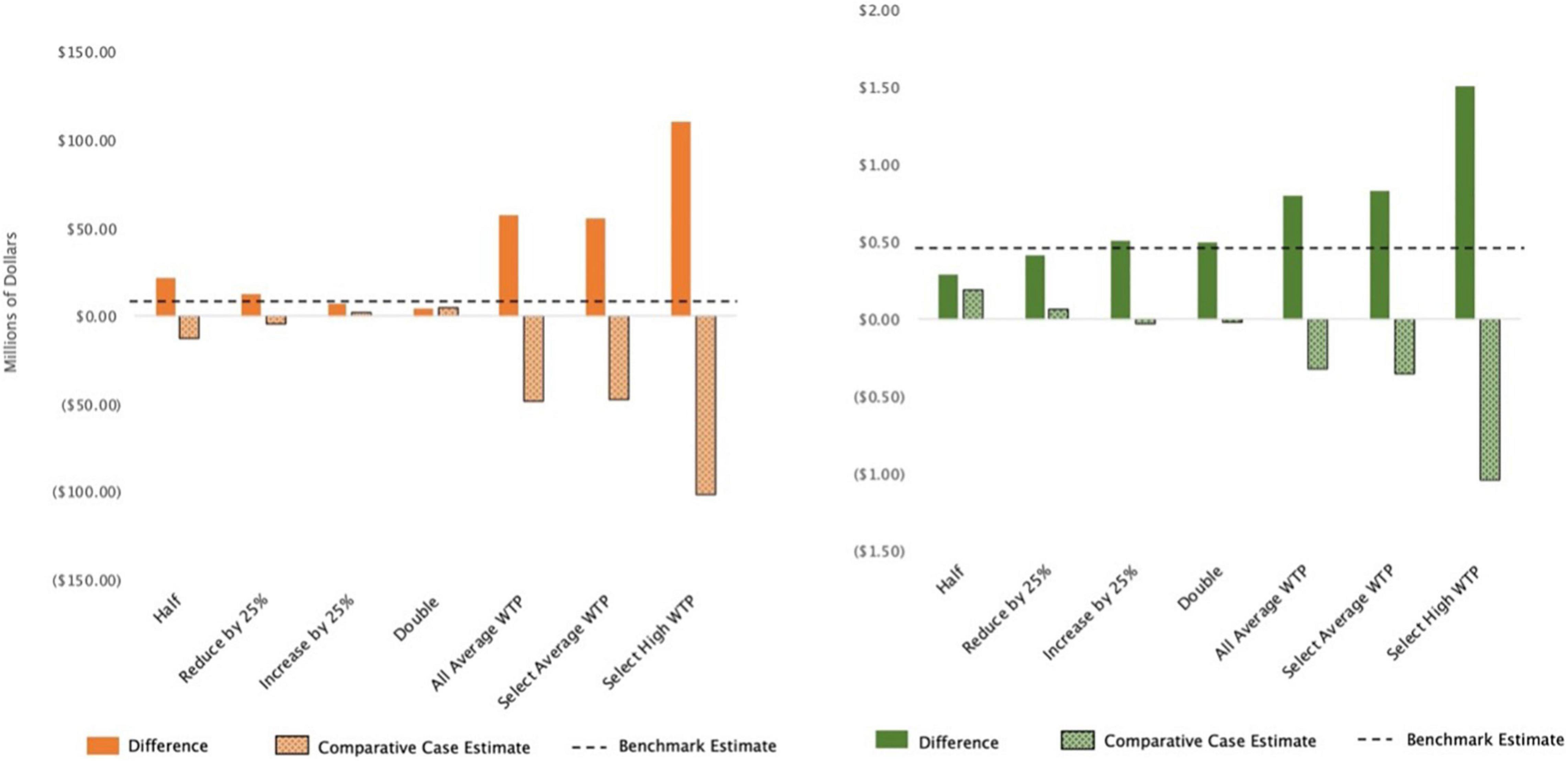
Figure 6. Estimates of social welfare loss in millions of dollars for select runs of additional analysis for fishermen responsiveness and preferences. The left panel is spatially heterogenous zones with Atlantis and the right panel is homogenous zones with non-Atlantis. Social welfare loss is measured as the net present value of the compensating variation. The four leftmost columns adjust the elasticity of substitution parameter: 0.45 and 0.675 make substitutions between species more difficult as compared to the benchmark, and 1.125 and 1.8 make them easier. The three rightmost columns adjust the willingness to pay values (WTP); the “All Average” run assigns the average WTP to all species, the “Select Average” run assigns the average WTP to the three species with unknown value, the “Select High” run assigns the highest WTP to the three species with unknown value.

Considered next are the results from the assessment of the values that the fishermen place on each species, or the willingness to pay (WTP) analysis. Social welfare losses increase across all ecological specifications (e.g., Figure 6, both panels) and all additional runs, when compared to the benchmark. Raising the value of the unknown species to the average (e.g., Figure 6, “All Average” column) or to the highest value generates higher social welfare losses because the species are on average negatively impacted by the invasion and costs to the fishermen, thereby, increase. In the case where all species are valued at the average, the increase in social welfare loss demonstrates the relative importance of understanding the value fishermen place on individual species. There are three species valued above the average in the benchmark run – Chinook salmon, Coho salmon, and steelhead. By assuming the average value, the costs of these three species are drawn down while the costs of all other species are pulled higher.

Protected Area Policy Analysis

The results of the policy analysis depend greatly on the ecological specification of the model. When the Atlantis model is used and zones are spatially heterogenous, the zone that will generate the greatest welfare improvement as a protected area is zone 3. Assigning zone 3 as the protected area reduces social welfare losses by approximately $2 million (Table 3). If the non-Atlantis model is used and the zones are spatially heterogenous, welfare losses are reduced most by designating zone 1 as the protected area; this saves approximately $121,000. Regardless of whether the Atlantis or non-Atlantis models are used, if zones are treated as spatially homogenous the zone expected to produce the greatest benefit as a protected area is zone 4. Designating zone 4 as a protected area saves nearly $100,000 when the non-Atlantis model is used and $1.94 million when the Atlantis model is used.

TABLE 3

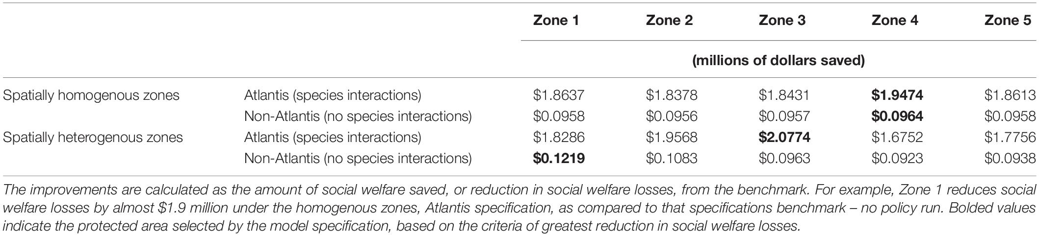
Table 3. Estimates of social welfare improvements (in millions of dollars) for each zone if it is designated as a protected area, under each ecological specification.

Discussion

There are two main drivers of the difference between the social welfare estimates when comparing the ecological specifications using the Atlantis model (with layers of species interactions) and the non-Atlantis model (without species interactions). First, the specifications that use the Atlantis model have a wider distribution of possible species biomass outcomes from the invasion because there are compounding or competing bigheaded carp effects for each species and dynamic interactions between species. Throughout the time frame of the invasion, most of the species experience at least some oscillations between periods of growth and decline. However, on net nearly all sportfishing species are negatively impacted by the Asian carp invasion. The magnitude of the implications differ depending on the ecological food web interactions. For fish species that spawn nearshore (i.e., lake whitefish, walleye, and yellow perch), the decreases in population biomass are significant and driven by direct food competition between bigheaded carp and larval fish of these species. Rainbow smelt are also significantly impacted by the invasion, because both they and bigheaded carp feed on zooplankters, compete for food, and share predations. Conversely, piscivorous fish species, such as burbot, Chinook salmon, Coho salmon, lake trout, and steelhead, are negatively impacted less across the time frame. Though the larval fish of these piscivorous species have minor food competition with bigheaded carp, this competition is offset by the fact that bigheaded carp become an extra food source for these species. This offsetting effect is dependent on the growth of the bigheaded carp, which in this simulation is slow due to food limitations and thus it took bigheaded carp longer to outgrow predators’ gape sizes.

Without these interactions, the non-Atlantis model predicts that each species either converges to a lower (or higher) steady state that simply depends on the magnitude of the bigheaded carp impact and whether the species is negatively (or positively) impacted (Figures 3, 7). Second, the magnitude of the ecological implications on each species are starkly different across settings. In the non-Atlantis setting, the bigheaded carp effects are rather small, so the changes in species biomass are also small (e.g., Figure 3, bottom panel), whereas the variation in impacts can be almost 20 times larger (e.g., Figure 3, rainbow smelt) when using the Atlantis model. Further, the biomass values from the bigheaded carp invasion differ greatly for species that hold high value to the fishermen across Atlantis and non-Atlantis specifications (e.g., Coho salmon, Chinook salmon, and steelhead). The representative fishermen cannot substitute as easily to the higher valued species in the Atlantis specifications because of the significant invasion implications on all the other species as well. In the non-Atlantis specification, however, the representative fishermen can make more tradeoffs because there are some species that increase in population biomass as a result of the invasion; the representative fisherman are able to use what they save on those species and spend it on the others.

FIGURE 7

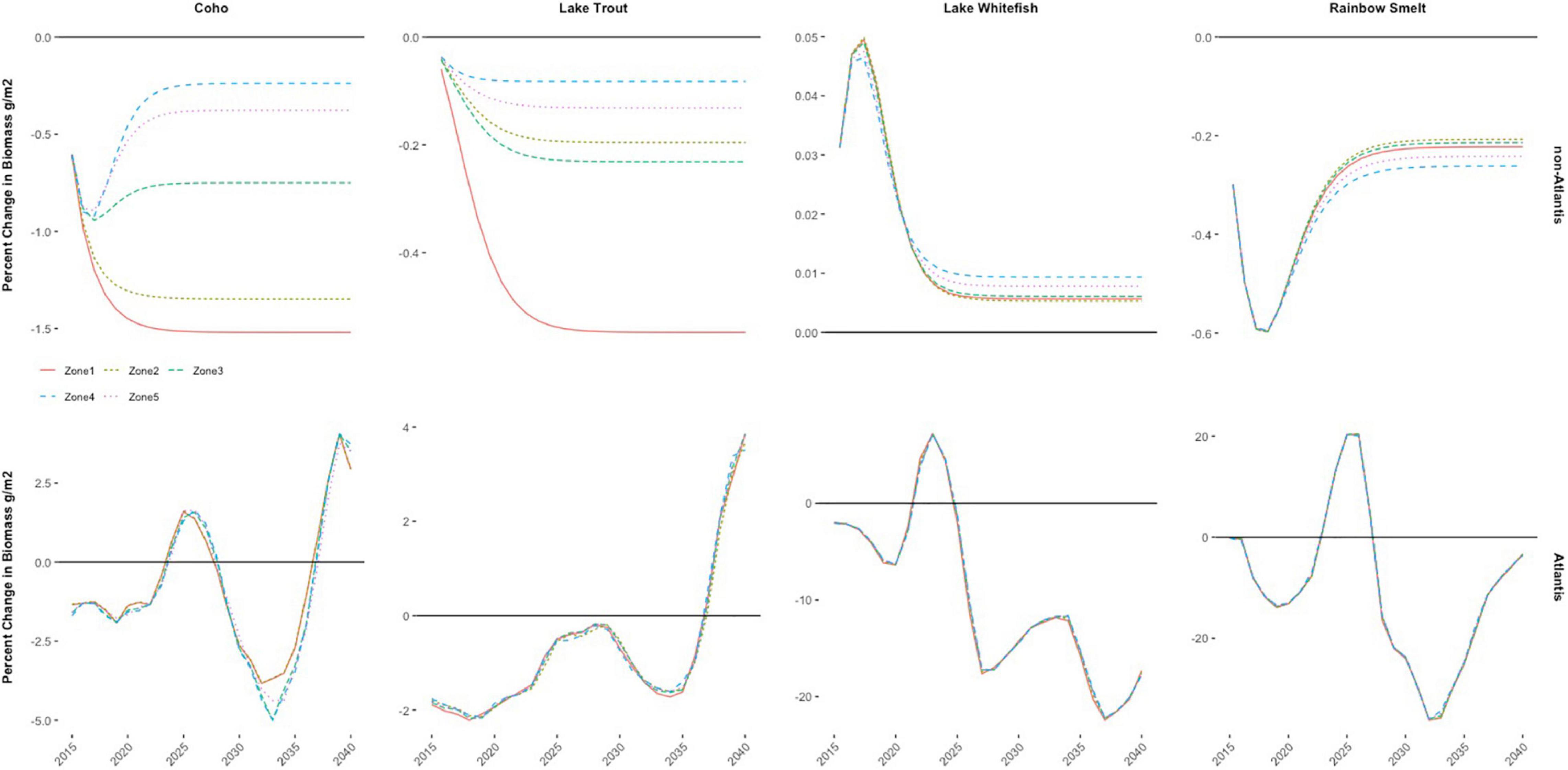
Figure 7. Yearly percent change in biomass for all Lake Michigan zones for select species.

In comparing spatially heterogenous zones to spatially homogenous zones, the results are understated when using the non-Atlantis model and overstated when using the Atlantis model. This is somewhat surprising as one might expect a similar aggregation to result in similar directions of divergence – either both overstated or both understated¹⁰. Note, however, that in making the assumption that all zones are the same ecologically some species will be present in zones where they would ecologically not exist in any significant volume of biomass (e.g., steelhead in zone 1). An implication of erroneous existence is overstated benefits associated with “greater” abundance of the species. If these existence benefits outweigh the aggregate costs of the invasion, the welfare losses will be understated and vice versa. For this specific analysis, when using the Atlantis model, the negative impacts of the bigheaded carp exacerbate the poor ecological condition in the zones and outweigh the benefit of additional existence. The reverse is true for the non-Atlantis specification. Although the differences in welfare estimates are small and the results of neither the Atlantis model, nor the non-Atlantis model are not significantly different in terms of the biomass for many species across space, the difference in social welfare calculations is a direct bias from aggregating and then assuming the average (Figure 7), implying that modeling the spatial ecological characteristics is important. In this specific analysis, the similarities across zones is caused by a lack of zone-specific spatial data for the non-Atlantis model, and by a predefined seasonal spatial distribution of fish species across zones that aggregates and redistributes species based on a set proportion over four seasons for the Atlantis model. Therefore, though the Atlantis model has different absolute biomass values for both bigheaded carp and the fishery species, based on the different productivities and food web interactions in the nearshore and offshore for each zone, the percent changes across the different zones will be similar.

When adapting how easy or difficult it is for the representative fishermen to substitute between species when responding to the invasion, the results are straightforward for most specifications: making it harder (or easier) to substitute makes fishermen worse off (or better off). The exception is for the non-Atlantis, spatially homogenous zones specification (Figure 6, right panel). The main question behind the result becomes, why would constraining substitution make the fishermen better off? The answer is in how social welfare is measured; the social welfare losses are calculated by comparing social wellbeing in the good state (i.e., the non-invasion state) to social wellbeing in the bad state (i.e., the invasion state), which is a relative measure that compares how different the values are. Being able to substitute less does in fact generate lower absolute levels of social welfare in both the non-invasion and invasion states, such that fishermen are in fact worse-off. But because the invasion effects are less severe when the non-Atlantis model is used and the zones are spatially homogenous, the relative difference between the levels of wellbeing in the two states is smaller.

The final point of discussion relates to the simplified and synthetic policy analysis, which considers designating one zone as a protected area that is not impacted from the bigheaded carp invasion. When the zones are treated as spatially homogenous – regardless of whether the Atlantis or non-Atlantis model is used – the model-suggested protected area is zone 4. Because the ecological characteristics are the same across zones, the ecological benefit (or value) of making any zone a protected area should, all else equal, be the same. However, the tradeoff between the ecological quality and the costs of traveling and purchases of quality-enhancing inputs – which are not aggregated – influence this result (Supplementary Table 1). Zone 4 is on average the costliest zone to travel to in terms of distance costs, and by making it the protected area the fishermen can tradeoff higher levels of quality for fewer trips; it becomes comparatively less expensive and generates the greatest benefit in terms of social welfare. This result, though, is biased due to the spatial homogeneity assumption and the issue of species having populations in zones where they ecologically are not well-established. For example, Chinook salmon do not have a well-established biomass in zone 4, yet the assumption that all zones are ecologically homogenous incorrectly assumes that Chinook salmon are established in the zone and overstates the benefits of making zone 4 a protected area (e.g., Supplementary Figure 9), especially in this instance because fishermen assign the highest willingness to pay values to Chinook salmon.

This bias is corrected to some extent when the zones account for spatial heterogeneity, but even still the designated protected area is different across the Atlantis and non-Atlantis models. The best zone to designate as a protected area is zone 3 under the Atlantis model specification. Zone 3 is one of the more ecologically diverse zones (i.e., all sportfishing species are established there) and one of the most impacted zones by the invasion in terms of increased costs of fishing (Figure 4, right column)¹¹. It is also one of the least costly to travel to, which altogether makes it the zone that creates the greatest value to the fishermen as a protected area in terms of bang for the buck. Using the more simplified, non-Atlantis model and maintaining spatial heterogeneity in zones, the best protected area designation is zone 1; under this specification, the population biomass implications are more negatively impacted by the bigheaded carp invasion as compared to the other zones (Figure 7).

Conclusion

The bioeconomic model presented in this paper assesses the potential social welfare losses associated with a bigheaded carp invasion and illustrates the biases that might result in those estimates if spatial characteristics or species-interactions are aggregated or excluded from the model and the implications of those biases on designing policy. Several key characteristics drive the results: the composition of the species in each lake zone, the relative economic importance or value of the species, and the compounding or competing effects of the interactions in levels of species biomass. When full ecological system and food web interactions are accounted for under the Atlantis model specification, the welfare losses are an order of magnitude larger than when the interactions are excluded in the non-Atlantis specification. This has important implications for policy. When using the social welfare estimates as a guide for how much or whether to invest in mitigation or conservation of metapopulations, incorrect estimates could lead to significant underfunding or overfunding by tens of millions of dollars. Further errors in policymaking were demonstrated through the simplified policy analysis, in which a designated protected area – lake zone – was selected based on the criteria of which zone reduced social welfare losses the most. When aggregating out spatially explicit ecological characteristics and treating all zones as spatially homogenous, the selection of the protected area was inherently biased. Though this bias is clear from this analysis because of the nature of the simplifying assumptions, the result tells a cautionary tale regarding aggregation and homogeneity assumptions. Altogether, the analysis reinforces the importance of including relevant species specifics and spatially explicit characteristics and supports the adage that the devil is in the details (e.g., Finnoff et al., 2005, 2019; Settle and Shogren, 2006; Wainger et al., 2010).

There are some caveats, which serve as motivation for future work. First, it is not clear that excluding species interactions – using the non-Atlantis model – will always understate the welfare outcome. Here, the effect of bigheaded carp on sportfishing species appears relatively minor (Zhang et al., 2016), but had the impact been much more severe, the results of the two ecological approaches could be starkly different. The simpler non-Atlantis model may predict species extinction while the more complex Atlantis model may show some attenuation of the impacts, further justifying the need to consider the spatial ecology surrounding the metapopulation. Similarly, the results across ecological regions may be much more distinct than those predicted by the Atlantis and non-Atlantis models. Because of data constraints and predefined seasonal distributions of fish data that is always proportional to the total population for the zones, the spatial implications across zones were very similar in this analysis, which leads to the next point. The model assumptions are not innocuous and should be thoughtfully considered, especially at the point of connection between the economic and ecological systems. There were further limitations on the availability of data, specifically related to fishing behavior. As a consideration for future research, data on differences in fishing behavior across representative fishermen and zones would improve the accuracy of welfare estimates. In addition, this analysis considers the implications of the invasion primarily on recreational fisherman, yet invasive species often impact additional segments of society (e.g., infrastructure, commercial fishing industries, transportation industries, labor markets and employment, or trade relationships). To understand full society-wide implications of the invasion, a complete economic model of the regional economy – firms, governments, trade, all consumer types, and market linkages – should be considered in general equilibrium setting.

Finally, from this analysis, a major underlying result is that a bigheaded carp invasion is likely to lead to social welfare loss. Regardless of whether the Atlantis or non-Atlantis model is used, most sportfishing species are on net negatively impacted by the invasion which increases the costs of fishing for each species across all zones for each recreational fisherman. The fishermen respond by reducing trips, quality purchases, and fishing across all zones due to budget limitations, and it is these lost fishing experiences that generate the social welfare losses. Therefore, the natural next step is to expand on this framework to address the above caveats and to begin assessing the ecological and economic efficacy of policy options being currently considered, rather than the synthetic and simplified analysis used herein for demonstrative purposes. The current policy recommendations, which are outside the scope of this analysis, include: (1) stocking economically important species that are impacted by the invasion to mitigate the effects of the invasion (Kao et al., 2018), (2) constructing barriers to keep bigheaded carp out of the lake (U.S. Geological Services, 2018; U.S. Army Corps of Engineers, 2019) or (3) developing a for profit market for bigheaded carp through commercial fishing or recreational tournaments (Illinois Department of Natural Resources, 2021; Kentucky Department of Fish and Wildlife Resources, 2021). Using a more comprehensive model to assess these policies would illustrate how the full economy would respond and if social welfare losses would indeed improve.

Data Availability Statement

The raw data supporting the conclusions of this article will be made available by the authors, without undue reservation.

Author Contributions

SB developed the economic model and simplified ecological model, calibrated the bioeconomic model, wrote the first draft of the manuscript, designed the comparative analysis, and generated figures and tables. HZ, DM, and ER collected the data used for the ecological models, developed and calibrated the Atlantis ecosystem model, and supplied the parameters for the simplified ecosystem model. HZ wrote on the ecological and spatial details of the invasion, the ecological Atlantis model section, and the Atlantis results. DM and ER provided feedback, clarifications, and edited and revised the latest manuscript. All authors contributed to the article and approved the submitted version.

Conflict of Interest

HZ was employed by the company Eureka Aquatic Research, LLC.

The remaining authors declare that the research was conducted in the absence of any commercial or financial relationships that could be construed as a potential conflict of interest.

Publisher’s Note

All claims expressed in this article are solely those of the authors and do not necessarily represent those of their affiliated organizations, or those of the publisher, the editors and the reviewers. Any product that may be evaluated in this article, or claim that may be made by its manufacturer, is not guaranteed or endorsed by the publisher.

Acknowledgments

The authors would like to thank the Great Lakes Fishery Trust for their support of this research through grant number 2015. Additionally, this work was supported by the Great Lakes Restoration Initiative (GLRI) from the U.S. Environmental Protection Agency through the U.S. Fish and Wildlife Service (grant number 2010-65-2). The authors would also like to thank the referees for their thoughtful comments and recommendations, which helped improve the manuscript.

Supplementary Material

The Supplementary Material for this article can be found online at: https://www.frontiersin.org/articles/10.3389/fevo.2021.703935/full#supplementary-material

Footnotes

1. ^ May also be known or referred to as Asian carp.
2. ^ The fisherman decision model is static and is solved each year for a different ecological perturbation; the ecological model is fully dynamic.
3. ^ This analysis is completed in a partial equilibrium setting. All market prices are considered exogenous to the representative fishermen and are unchanging in this framework, though a set of prices – namely those associated with recreational fishing quality, species biomass, and overall fishing costs can fluctuate as the fishermen alter their behavior.
4. ^ Though not used in this analysis, seasonal spatial distributions of species could also incorporate the information of migrations within the lake or food availability.
5. ^ www.IMPLAN.com
6. ^ Parameters for the full bioeconomic model are shown in Supplementary Table 1. Also, to distinguish between variables and parameters in the economic model, variables are highlighted in the boxes of the decision-making tree (Figure 2).
7. ^ The discount rate was arbitrarily chosen but sensitivity analysis in which the rate was cut in half and doubled, showed that only the magnitude of the social welfare estimates change, not the direction of the results or the underlying takeaways.
8. ^ This policy analysis does not include implementation related costs (e.g., construction of barriers, or control costs); the current analysis focuses only bias in site selection due to simplified space and species interactions.
9. ^ The increase in biomass for these two species is directly a result of the parameters used from Zhang et al. (2016).
10. ^ By dealing with averages across five zones, an outlier type of either extreme could skew the overall impacts toward that extreme.
11. ^ Relative to all other zones, zone 3 is only ecological slightly better off than zone 2 for the low-income household division and zones 1 and 2 for the middle-income division.

References

Aadland, D., Sims, C., and Finnoff, D. (2015). Spatial dynamics of optimal management in bioeconomic systems. Comput. Econ. 45, 545–577. doi: 10.1007/s11538-014-0003-2

PubMed Abstract | CrossRef Full Text | Google Scholar

Albers, H. J. (1996). Modeling ecological constraints on tropical forest management: spatialinterdependence, irreversibility, and uncertainty. J. Environ. Econ. Manage. 30, 73–94. doi: 10.1006/jeem.1996.0006

CrossRef Full Text | Google Scholar

Albers, H. J., Fischer, C., and Sanchirico, J. N. (2010). Invasive species management in a spatially heterogeneous world: effects of uniform policies. Resour. Energy Econ. 32, 483–499.

Google Scholar

Alsip, P. J., Zhang, H., Rowe, M. D., Mason, D. M., Rutherford, E. S., Riseng, C. M., et al. (2019). Lake Michigan’s suitability for bigheaded carp: the importance of diet flexibility and subsurface habitat. Freshw. Biol. 64, 1921– 1939.

Google Scholar

Alsip, P. J., Zhang, H., Rowe, M. D., Rutherford, E., Mason, D. M., Riseng, C., et al. (2020). Modeling the interactive effects of nutrient loads, meteorology, and invasive mussels on suitable habitat for Bighead and Silver Carp in Lake Michigan. Biol. Invasion. 22, 2763–2785.

Google Scholar

Anderson, C. A. (2016). Diet Analysis of Native Predatory Fish to Investigate Predation of Juvenile Asian Carp. Macomb, IL: Western Illinois University.

Google Scholar

Audzijonyte, A., Gorton, R., Kaplan, I., and Fulton, E. A. (2017). Atlantis User’s Guide Part I: General Overview, Physics and Ecology. Clayton, Australia: CSIRO Publishing.

Google Scholar

Ballard, C. L., Fullerton, D., Shoven, J. B., and Whalley, J. (1985). A General Equilibrium Model for Tax Policy Evaluation. Chicago, IL: University of Chicago Press, 1–5.

Google Scholar

Beletsky, D., and Schwab, D. (2008). Climatological circulation in Lake Michigan. Geophys. Res. Lett. 35:L21604.

Google Scholar

Bockstael, N. E. (1996). Modeling economics and ecology: the importance of a spatial perspective. Am. J. Agric. Econ. 78, 1168–1180.

Google Scholar

Bockstael, N. E., and McConnell, K. E. (1981). Theory and estimation of the household production function for wildlife recreation. J. Environ. Econ. Manage. 8, 199–214. doi: 10.1016/0095-0696(81)90037-1

CrossRef Full Text | Google Scholar

Brenden, T. O., and Bence, J. R. (2009). A Model Based Evaluation of How Stocking Oncorhynchus Influences the Fish Communities of Lakes Huron and Ontario. 2009 Project Completion Report. Ann Arbor, MI: Great Lakes Fishery Commission.

Google Scholar

Brown, G., and Roughgarden, J. (1997). A metapopulation model with private property and a common pool. Ecol. Econ. 22, 65–71. doi: 10.1016/s0921-8009(97)00564-8

CrossRef Full Text | Google Scholar

Brown, R. W., Taylor, W. W., and Assel, R. A. (1993). Factors affecting the recruitment of lake whitefish in two areas of northern Lake Michigan. J. Great Lakes Res. 19, 418–428. doi: 10.1016/s0380-1330(93)71229-0

CrossRef Full Text | Google Scholar

Carbone, J. C., and Smith, V. K. (2013). Valuing nature in a general equilibrium. J. Environ. Econ. Manage. 66, 72–89.

Google Scholar

Cooke, S. L., and Hill, W. R. (2010). Can filter−feeding Asian carp invade the Laurentian Great Lakes? A bioenergetic modelling exercise. Freshw. Biol. 55, 2138–2152. doi: 10.1111/j.1365-2427.2010.02474.x

CrossRef Full Text | Google Scholar

Cooke, S. L., Hill, W. R., and Meyer, K. P. (2009). Feeding at different plankton densities alters invasive bighead carp (Hypophthalmichthys nobilis) growth and zooplankton species composition. Hydrobiologia 625, 185–193. doi: 10.1007/s10750-009-9707-y

CrossRef Full Text | Google Scholar

Costello, C., and Polasky, S. (2008). Optimal harvesting of stochastic spatial resources. J. Environ. Econ. Manage. 56, 1–18. doi: 10.1016/j.jeem.2008.03.001

CrossRef Full Text | Google Scholar

DeBoer, J. A., Anderson, A. M., and Casper, A. F. (2018). Multi−trophic response to invasive silver carp (Hypophthalmichthys molitrix) in a large floodplain river. Freshw. Biol. 63, 597–611. doi: 10.1111/fwb.13097

CrossRef Full Text | Google Scholar

EPA NHEERL (2003). Level III and IV Ecoregions of the Continental United States. Corvallis, OR. Available online at: https://www.epa.gov/eco-research/level-iii-and-iv-ecoregions-continental-united-states (accessed October 10, 2021).

Google Scholar

Epanchin-Niell, R. S. (2017). Economics of invasive species policy and management. Biol. Invasion. 19, 3333–3354. doi: 10.1007/s10530-017-1406-4

CrossRef Full Text | Google Scholar

Epanchin-Niell, R. S., and Wilen, J. E. (2012). Optimal spatial control of biological invasions. J. Environ. Econ. Manage. 63, 260–270. doi: 10.1016/j.jeem.2011.10.003

CrossRef Full Text | Google Scholar

Finnoff, D., Brockmann, S., Zhang, H., Rutherford, E., and Mason, D. (2019). Forecasting Biological and Economic Impacts of Aquatic Invasive Species in Lake Michigan, Great Lakes Fishery Trust, Technical Report. Lansing, MI: Great Lakes Fishery Trust.

Google Scholar

Finnoff, D., McIntosh, C., Shogren, J. F., Sims, C., and Warziniack, T. (2010). Invasive species and endogenous risk. Annu. Rev. Resour. Econ. 2, 77–100. doi: 10.1146/annurev.resource.050708.144212

CrossRef Full Text | Google Scholar

Finnoff, D., Shogren, J. F., Leung, B., and Lodge, D. (2005). The importance of bioeconomic feedback in invasive species management. Ecol. Econ. 52, 367–381. doi: 10.1016/j.ecolecon.2004.06.020

CrossRef Full Text | Google Scholar

Fulton, E. A., Link, J. S., Kaplan, I. C., Savina-Rolland, M., Johnson, P., Ainsworth, C., et al. (2011). Lessons in modelling and management of marine ecosystems: the Atlantis experience. Fish Fish. 12, 171–188.

Google Scholar

Fulton, E. A., Parslow, J. S., Smith, A. D., and Johnson, C. R. (2004). Biogeochemical marine ecosystem models II: the effect of physiological detail on model performance. Ecol. Modell. 173, 371–406. doi: 10.1016/j.ecolmodel.2003.09.024

CrossRef Full Text | Google Scholar

Hanley, N., and Roberts, M. (2019). The economic benefits of invasive species management. People Nat. 1, 124–137. doi: 10.1002/pan3.31

CrossRef Full Text | Google Scholar

Hastings, A. (2013). Population Biology: Concepts and Models. Berlin: Springer Science & Business Media.

Google Scholar

Illinois Department of Natural Resources (2021). Illinois Park and Recreational Facility Construction Grant Program (PARC). Available online at: https://www2.illinois.gov/dnr/grants/Documents/2021_PARC_Manual.pdf (accessed September 28, 2021).

Google Scholar

IMPLAN (2014). IMPLAN Group LLC, IMPLAN System (Data and Software),16905 Northcross Dr., Suite 120, Huntersville, NC 28078. Available online at: www.implan.com.

Google Scholar

Kao, Y. C., Rogers, M. W., and Bunnell, D. B. (2018). Evaluating stocking efficacy in an ecosystem undergoing oligotrophication. Ecosystems 21, 600–618. doi: 10.1007/s10021-017-0173-5

CrossRef Full Text | Google Scholar

Kaplan, I. C., Levin, P. S., Burden, M., and Fulton, E. A. (2010). Fishing catch shares in the face of global change: a framework for integrating cumulative impacts and single species management. Can. J. Fish Aquat. Sci. 67, 1968–1982. doi: 10.1139/f10-118

PubMed Abstract | CrossRef Full Text | Google Scholar

Kentucky Department of Fish and Wildlife Resources (2021). Invasive Carp Information. Available online at: https://fw.ky.gov/Fish/Pages/Invasive-Carp-Information.aspx (accessed September 28, 2021).

Google Scholar

Kolar, C. S., Chapman, D. C., Courtenay, W. R. Jr., Housel, C. M., Williams, J. D., and Jennings, D. P. (2007). Bigheaded Carps: A Biological Synopsis and Environmental Risk Assessment. Bethesda, MD: American Fisheries Society.

Google Scholar

Kolstad, C. (2011). Environmental Economics. Oxford: Oxford University Press.

Google Scholar

Leung, B., Lodge, D. M., Finnoff, D., Shogren, J. F., Lewis, M. A., and Lamberti, G. (2002). An ounce of prevention or a pound of cure: bioeconomic risk analysis of invasive species. Proc. R. Soc. Lond. B Biol. Sci. 269, 2407–2413. doi: 10.1098/rspb.2002.2179

PubMed Abstract | CrossRef Full Text | Google Scholar

Madenjian, C. P., Bunnell, D. B., Warner, D. M., Pothoven, S. A., Fahnenstiel, G. L., Nalepa, T. F., et al. (2015). Changes in the Lake Michigan food web following dreissenid mussel invasions: a synthesis. J. Great Lakes Res. 41, 217–231. doi: 10.1016/j.jglr.2015.08.009

CrossRef Full Text | Google Scholar

Melstrom, R. T., and Lupi, F. (2013). Valuing recreational fishing in the Great Lakes. N. Am. J. Fish Manag. 33, 1184–1193. doi: 10.1080/02755947.2013.835293

CrossRef Full Text | Google Scholar

Miller, T. J., Crowder, L. B., Rice, J. A., and Binkowski, F. P. (1992). Body size and the ontogeny of the functional response in fishes. Can. J. Fish. Aquat. Sci. 49, 805–812. doi: 10.1139/f92-091

PubMed Abstract | CrossRef Full Text | Google Scholar

Olsen, E., Kaplan, I. C., Ainsworth, C., Fay, G., Gaichas, S., Gamble, R., et al. (2018). Ocean futures under ocean acidification, marine protection, and changing fishing pressures explored using a worldwide suite of ecosystem models. Front. Mar. Sci. 5:64. doi: 10.3389/fmars.2018.00064

CrossRef Full Text | Google Scholar

Pendleton, R. M., Schwinghamer, C., Solomon, L. E., and Casper, A. F. (2017). Competition among river planktivores: are native planktivores still fewer and skinnier in response to the Silver Carp invasion? Environ. Biol. Fishes 100, 1213–1222. doi: 10.1007/s10641-017-0637-7

CrossRef Full Text | Google Scholar

Perrings, C., Dalmazzone, S., and Williamson, M. H. (2000). The Economics of Biological Invasions. Cheltenham: Edward Elgar Publishing.

Google Scholar

Phelps, Q. E., Tripp, S. J., Bales, K. R., James, D., Hrabik, R. A., and Herzog, D. P. (2017). Incorporating basic and applied approaches to evaluate the effects of invasive Asian Carp on native fishes: a necessary first step for integrated pest management. PLoS One 12:e0184081. doi: 10.1371/journal.pone.0184081

PubMed Abstract | CrossRef Full Text | Google Scholar

Pimentel, D., Lach, L., Zuniga, R., and Morrison, D. (2000). Environmental and economic costs of nonindigenous species in the United States. BioScience 50, 53–65. doi: 10.1641/0006-3568(2000)050[0053:eaecon]2.3.co;2

CrossRef Full Text | Google Scholar

Pimentel, D., Zuniga, R., and Morrison, D. (2005). Update on the environmental and economic costs associated with alien-invasive species in the United States. Ecol. Econ. 52, 273–288.

Google Scholar

Ray, W. J., and Corkum, L. D. (1997). Predation of zebra mussels by round gobies, Neogobius melanostomus. Environ. Biol. Fishes 50, 267–273. doi: 10.1023/a:1007379220052

CrossRef Full Text | Google Scholar

Riseng, C. M., Wehrly, K. E., Wang, L., Rutherford, E. S., McKenna, J. E. Jr., Johnson, L. B., et al. (2017). Ecosystem classification and mapping of the Laurentian Great Lakes. Can. J. Fish. Aquat. Sci. 75, 1693–1712.

Google Scholar

Rogers, M. W., Bunnell, D. B., Madenjian, C. P., and Warner, D. M. (2014). Lake Michigan offshore ecosystem structure and food web changes from 1987 to 2008. Can. J. Fish. Aquat. Sci. 71, 1072–1086. doi: 10.1139/cjfas-2013-0514

PubMed Abstract | CrossRef Full Text | Google Scholar

Rutherford, E. S., Zhang, H., Kao, Y. C., Mason, D. M., Shakoor, A., Bouma-Gregson, K., et al. (2021). Potential effects of bigheaded carps on four Laurentian Great Lakes food webs. N. Am. J. Fish. Manag. 41, 999–1019.

Google Scholar

Rutherford, T. (2002). Lecture Notes on Constant Elasticity Functions. Boulder, CO: University of Colorado.

Google Scholar

Sanchirico, J., Wilen, J. E., and Coleman, C. (2010). Optimal rebuilding of a metapopulation. Am. J. Agric. Econ. 92, 1087–1102. doi: 10.1093/ajae/aaq045

CrossRef Full Text | Google Scholar

Sanchirico, J. N., and Wilen, J. E. (1999). Bioeconomics of spatial exploitation in a patchy environment. J. Environ. Econ. Manage. 37, 129–150. doi: 10.1006/jeem.1998.1060

CrossRef Full Text | Google Scholar

Settle, C., and Shogren, J. F. (2006). Does integrating economic and biological systems matter for public policy? The case of Yellowstone Lake. Top Econ. Anal. Policy 6, 1352–1352.

Google Scholar

Simberloff, D., Martin, J. L., Genovesi, P., Maris, V., Wardle, D. A., Aronson, J., et al. (2013). Impacts of biological invasions: what’s what and the way forward. Trends Ecol. Evol. 28, 58–66. doi: 10.1016/j.tree.2012.07.013

PubMed Abstract | CrossRef Full Text | Google Scholar

Solomon, L. E., Pendleton, R. M., Chick, J. H., and Casper, A. F. (2016). Long-term changes in fish community structure in relation to the establishment of Asian carps in a large floodplain river. Biol. Invasion. 18, 2883–2895. doi: 10.1007/s10530-016-1180-8

CrossRef Full Text | Google Scholar

U.S. Army Corps of Engineers (2019). Chief of Engineers Approves Plan for Preventing Asian Carp Transfer Into Great Lakes. Available online at: https://www.mvr.usace.army.mil/Media/News-Releases/Article/1857381/chief-of-engineers-approves-plan-for-preventing-asian-carp-transfer-into-great/ (accessed September 28, 2021).

Google Scholar

U.S. Census Bureau (2018). American Community Survey, 2016 1-Year Estimates, Data DP03 using American FactFinder. Available online at: http://factfinder.census.gov (accessed October 1, 2018).

Google Scholar

U.S. Department of the Interior, Fish and Wildlife Service, and U.S. Department of Commerce (2011). 2011 National Survey Of Fishing, Hunting, and Wildlife-Associated Recreation. US Department of the Interior, Fish and Wildlife Service, and US Department of Commerce, Bureau of the Census. Washington, DC: US Government Printing Office.

Google Scholar

U.S. Fish and Wildlife Service (2012). The Cost of Invasive Species. Available online at: https://www.fws.gov/verobeach/PythonPDF/CostofInvasivesFactSheet.pdf (accessed September 28, 2021).

Google Scholar

U.S. Geological Services (2018). Asian Carp Integrate Control and Containment. Available online at: https://www.usgs.gov/special-topic/glrist/science/asian-carp-integrated-control-and-containment?qt-science_center_objects=0#qt-science_center_objects (accessed September 28, 2021).

Google Scholar

Varian, H. R. (1992). Microeconomic Analysis. New York, NY: WW Norton.

Google Scholar

Wainger, L. A., King, D. M., Mack, R. N., Price, E. W., and Maslin, T. (2010). Can the concept of ecosystem services be practically applied to improve natural resource management decisions? Ecol. Econ. 69, 978–987. doi: 10.1111/cobi.12560

PubMed Abstract | CrossRef Full Text | Google Scholar

Warziniack, T., Haight, R. G., Yemshanov, D., Apriesnig, J. L., Holmes, T. P., Countryman, A. M., et al. (2021). “Economics of invasive species,” in Invasive Species in Forests and Rangelands of the United States, eds T. M. Poland, T. Patel-Weynand, D. M. Finch, C. F. Miniat, D. C. Hayes, and V. M. Lopez (Cham: Springer), 305.

Google Scholar

Wittmann, M. E., Cooke, R. M., Rothlisberger, J. D., Rutherford, E. S., Zhang, H., Mason, D. M., et al. (2015). Use of structured expert judgment to forecast invasions by bighead and silver carp in Lake Erie. Conserv. Biol. 29, 187–197. doi: 10.1111/cobi.12369

PubMed Abstract | CrossRef Full Text | Google Scholar

Zhang, H., Rutherford, E. S., Mason, D. M., Breck, J. T., Wittmann, M. E., Cooke, R. M., et al. (2016). Forecasting the impacts of silver and bighead carp on the Lake Erie food web. Trans. Am. Fish. Soc. 145, 136–162.

Google Scholar